Quantum fluctuating geometries and the information paradox

Abstract

We study Hawking radiation on the quantum space-time of a collapsing null shell. We use the geometric optics approximation as in Hawking’s original papers to treat the radiation. The quantum space-time is constructed by superposing the classical geometries associated with collapsing shells with uncertainty in their position and mass. We show that there are departures from thermality in the radiation even though we are not considering back reaction. One recovers the usual profile for the Hawking radiation as a function of frequency in the limit where the space-time is classical. However, when quantum corrections are taken into account, the profile of the Hawking radiation as a function of time contains information about the initial state of the collapsing shell. More work will be needed to determine if all the information can be recovered. The calculations show that non-trivial quantum effects can occur in regions of low curvature when horizons are involved, as for instance advocated in the firewall scenario.

I Introduction

Black hole evaporation is perhaps the salient problem of fundamental physics nowadays, since it tests gravity, quantum field theory and thermodynamics in their full regimes. Hawking’s calculation showing that black holes radiate a thermal spectrum initiated the study of this phenomenon. However, the calculation assumes a fixed given space-time, whereas it is expected that the black hole loses mass through the radiation and eventually evaporates completely. Associated with the evaporation process is the issue of loss of information, whatever memory of what formed the black hole is lost as it evaporates in a thermal state characterized by only one number, its temperature. Having a model calculation that follows the formation of a black hole and its evaporation including quantum effects would be very useful to gain insights into the process. Here we would like to present such a model. We will consider the collapse of a null shell. The associated space-time is very simple: it is Schwarzschild outside the shell and flat space-time inside. We will consider a quantum evolution of the shell with uncertainty in its position and momentum and we will superpose the corresponding space-times to construct a quantum space-time. On it we will study the emission of Hawking radiation in the geometric optics approximation. We will see that in the classical limit one recovers ordinary Hawking radiation. However, when quantum fluctuations of the collapsing shell are taken into account we will see that non vanishing off-diagonal terms appear in the density matrix representing the field. The correlations and the resulting profile of particle emission are modulated with information about the initial quantum state of the shell, showing that information can be retrieved. At the moment we do not know for sure if all information is retrieved.

The model we will consider is motivated in previous studies of the collapse of a shell lwf ; hajicek ; shellqg . In all these, an important role is played by the fact that that there are two conjugate Dirac observables. One of them is the ADM mass of the shell. The other is related to the position along scri minus from which the shell was sent inwards. These studies are of importance because they show that the quantization of the correct Dirac observables for the problem lead to a different scenario than those considered in the past using other reduced models of the fluctuating horizon of the shell (see for instance medvedetal ).

The organization of this paper is as follow. In the next section we review the calculation of the radiation with a background given by a classical collapsing shell for late times in the geometric optics approximation, mostly to fix notation to be used in the rest of the work. In section 3 we will remove the late time approximation providing an expression of the radiation of the shell for all times. We will also derive a closed expression for the distribution of radiation as a function of the position of the detector on scri plus. We will show that when the shell approaches the horizon the usual thermal radiation is recovered. We will see that the use of the complete expression for all times is useful when one considers the case of fluctuating horizons in the early (non-thermal) phases of the radiation prior to the formation of a horizon. This element had been missed in previous calculations that tried to incorporate such effects. In section 4 we will consider a quantum shell and the radiation it produces, we will proceed in two stages. First we will compute the expectation value of Bogoliubov coefficients. This will allow to explain in a simple case the technique that shall be used. However, the calculation of the number of particles produced requires the expectation value of a product of Bogoliubov coefficients. In section 5 we consider the calculation of the density matrix in terms of the product of Bogoliubov operators and show that the radiation profile reproduces the usual thermal spectrum for the diagonal elements of the density matrix, but with some departures due to the fluctuations in the mass of the shell. In section 6 we will show that it differs significantly from the product of the expectation values, particularly in the late stages of the process. In section 7 we will analyze coherences that vanish in the classical case and show they are non-vanishing and that allow information from the initial state of the shell to be retrieved. We end with a summary and outlook.

II Radiation of a collapsing classical shell

Here we reproduce well known results h74 for the late time radiation of a collapsing classical shell in a certain amount of detail since we will use them later on. The metric of the space-time is given by

$$ds^{2}=-\left(1-\frac{2M\theta(v-v_{s})}{r}\right)dv^{2}+2dvdr+r^{2}d\Omega^{2},$$ (1)

where $v_{s}$ represents the position of the shell (in ingoing Eddington–Finkelstein coordinates) and $M$ its mass . Throughout this paper we will be working in the geometric optics approximation (i.e. large frequencies). In this geometry, light rays that leave $I^{-}$ with coordinate $v$ less than $v_{0}=v_{s}-4M$ can escape to $I^{+}$ and the rest are trapped in the black hole that forms. Therefore $v=v_{0}$ defines the position of the event horizon. We will use that a light ray departing from $I^{-}$ with $v<v_{0}$ reaches $I^{+}$ at an outgoing Eddington–Finkelstein coordinate $u$ given by

$$u(v)=v-4M\ln\left(\frac{v_{0}-v}{4M_{0}}\right),$$ (2)

where $M_{0}$ is an arbitrary parameter that is usually chosen as $M_{0}=M$, stemming from the definition of the tortoise coordinate which involves a constant of integration.

Figure 1: The Penrose diagram of a classical collapsing shell. $v_{s}$ indicates the position at scri minus from which the shell is sent in. Light rays sent in to the left of $v_{0}$ make it to scri plus, whereas rays sent in to the right of $v_{0}$ get trapped in the black hole.

On the above metric we would like to study Hawking radiation corresponding to a scalar field. We consider the “in” vacuum associated with the mode expansion $\psi_{lm\omega^{\prime}}$. The asymptotic form of the modes in $I^{-}$ is given by,

$$\psi_{lm\omega^{\prime}}(r,v,\theta,\phi)=\frac{e^{-i\omega^{\prime}v}}{4\pi r\sqrt{\omega^{\prime}}}Y_{lm}(\theta,\phi),$$

and the “out” vacuum corresponding to modes $\chi_{lm\omega}$ with asymptotic form in $I^{+}$ given by

$$\chi_{lm\omega}(r,u,\theta,\phi)=\frac{e^{-i\omega u}}{4\pi r\sqrt{\omega}}Y_{lm}(\theta,\phi).$$

The geometric optics approximation consists of mapping the modes $\chi_{lm\omega}$ into $I^{-}$ as

$$\frac{e^{-i\omega u(v)}}{4\pi r\sqrt{\omega}}Y_{lm}(\theta,\phi),$$

where $u\left(v\right)$ is determined by the path of the light rays that emanate from $I^{-}$ at time $v$ and arrive in $I^{+}$ at $u(v)$.

The Bogoliubov coefficients are given by the Klein-Gordon inner products,

$$\alpha_{\omega\omega^{\prime}}=\left\langle\chi_{lm\omega},\psi_{lm\omega^{\prime}}\right\rangle,$$

$$\beta_{\omega\omega^{\prime}}=-\left\langle\chi_{lm\omega},\psi_{lm\omega^{\prime}}^{*}\right\rangle.$$

They can be computed in the geometric optics approximation projecting the out modes in $I^{-}$ and substituting the expression for $u(v)$. Focusing on the beta coefficient we get,

$$\beta_{\omega\omega^{\prime}}=-\frac{1}{2\pi}\sqrt{\frac{\omega^{\prime}}{\omega}}{\int_{-\infty}^{v_{0}}}dve^{-i\omega\left[v-4M\ln\left(\frac{v_{0}-v}{4M_{0}}\right)\right]-i\omega^{\prime}v}.$$ (3)

Since we are considering modes that are not normalizable one in general will get divergences. This can be dealt with by considering wave-packets localized in both frequency and time. For example,

$$\chi_{lmn\omega_{j}}=\frac{1}{\sqrt{\epsilon}}{\int_{j\epsilon}^{\left(j+1\right)\epsilon}}d\omega e^{u_{n}\omega i}\chi_{lm\omega},$$ (4)

constitute an orthonormal countable complete basis of packets centered in time $u_{n}=\frac{2\pi n}{\epsilon}$, and in frequency $\omega_{j}=\left(j+\frac{1}{2}\right)\epsilon$.

The original Hawking calculation assumes that the rays depart just before the formation of the horizon and arrive at $I^{+}$ at late times. In that case one can approximate,

$$u(v)=v-4M\ln\left(\frac{v_{0}-v}{4M_{0}}\right)\approx v_{0}-4M\ln\left(\frac{v_{0}-v}{4M_{0}}\right).$$

Defining a new integration variable $x=\frac{v_{0}-v}{4M_{0}}$ one gets

$$\beta_{\omega\omega^{\prime}}=-\frac{4M_{0}}{2\pi}\sqrt{\frac{\omega^{\prime}}{\omega}}\underset{\epsilon\to 0}{\lim}{\int_{0}^{\infty}}dxe^{-i\omega\left[v_{0}-4M\ln\left(x\right)\right]-i\omega^{\prime}\left(v_{0}-4M_{0}x\right)}e^{-\epsilon x},$$ (5)

where the last factor was added to make the integral convergent since we have used plane waves instead of localized packets as the basis of modes, following Hawking’s original derivation. Using the identity

$${\int_{0}^{\infty}}dxe^{a\ln\left(x\right)}e^{-bx}=e^{-(1+a)\ln\left(b\right)}\Gamma\left(1+a\right),\quad Re(b)>0,$$ (6)

and the usual prescription for the logarithm of a complex variable we can take the limit and get

$$\beta_{\omega\omega^{\prime}}=-\frac{i}{2\pi}\frac{e^{-i\left(\omega+\omega^{\prime}\right)v_{0}}}{\sqrt{\omega\omega^{\prime}}}e^{-2\pi M\omega}\Gamma\left(1+4M\omega i\right)e^{-4M\omega i\ln(4M_{0}\omega^{\prime})}.$$ (7)

Now from the Bogoliubov coefficients we can calculate the expectation value of the number of particles per unit frequency detected at scri using

$$\left\langle N^{H}_{\omega}\right\rangle={\int}_{0}^{\infty}d\omega^{\prime}\beta_{\omega\omega^{\prime}}\beta_{\omega\omega^{\prime}}^{*}=\frac{1}{4\pi^{2}\omega}e^{-4\pi M\omega}\left|\Gamma\left(1+4M\omega i\right)\right|^{2}{\int_{0}^{\infty}}d\omega^{\prime}\frac{1}{\omega^{\prime}},$$

where we added the superscript “$H$” to indicate this is the calculation originally carried out by Hawking.

The pre-factor is computed using the identity

$$\Gamma\left(1+z\right)\Gamma\left(1-z\right)=\frac{z\pi}{\sin\left(z\pi\right)},$$

with $z=4M\omega i$, which leads to,

$$\left|\Gamma\left(1+4M\omega i\right)\right|^{2}=\frac{8M\pi\omega}{e^{+4M\omega\pi}-e^{-4M\omega\pi}}.$$

To handle the divergent integral we note that

$${\int_{0}^{\infty}}d\omega^{\prime}\frac{1}{\omega^{\prime}}=\underset{\alpha\to 0}{\lim}{\int_{0}^{\infty}}d\omega^{\prime}\frac{1}{\omega^{\prime}}e^{i4M\alpha\ln(\omega^{\prime})}=\left[\begin{array}[]{l}y=\ln\left(\omega^{\prime}\right)\\ dy=\frac{d\omega^{\prime}}{\omega^{\prime}}\end{array}\right]=$$

$$=\underset{\alpha\to 0}{\lim}{\int_{0}^{\infty}}dye^{i4M\alpha y}=\frac{1}{4M}\delta\left(0\right).$$

Therefore,

$$\langle N_{\omega}^{H}\rangle=\frac{1}{e^{8M\omega\pi}-1}\frac{4M}{2\pi}{\int_{0}^{\infty}}d\omega^{\prime}\frac{1}{\omega^{\prime}}=\frac{1}{e^{8M\omega\pi}-1}\delta\left(0\right).$$ (8)

Again, the results is infinite because we considered plane waves. The time of arrival has infinite uncertainty and we are therefore adding up all the particles generated for an infinite amount of time. To deal with this we can consider wave-packets centered in time $u_{n}$ and frequency $\omega_{j}$ for which the Bogoliubov coefficients are,

$$\beta_{\omega_{j}\omega^{\prime}}=\frac{1}{\sqrt{\epsilon}}{\int_{j\epsilon}^{{\left(j+1\right)\epsilon}}}d\omega e^{u_{n}\omega i}\beta_{\omega\omega^{\prime}}.$$

We start computing the density matrix

$$\rho^{H}_{\omega_{1},\omega_{2}}={\int_{0}^{\infty}}d\omega^{\prime}\beta_{\omega_{1}\omega^{\prime}}\beta_{\omega_{2}\omega^{\prime}}^{*}=\frac{1}{4\pi^{2}\sqrt{\omega_{1}\omega_{2}}}e^{-i\left(\omega_{1}-\omega_{2}\right)v_{0}}e^{-2\pi M\left(\omega_{1}+\omega_{2}\right)}\Gamma\left(1+4M\omega_{1}i\right)\Gamma\left(1-4M\omega_{2}i\right)\times$$

$$\times{\int_{0}^{\infty}}d\omega^{\prime}\frac{1}{\omega^{\prime}}e^{-4M\left(\omega_{1}-\omega_{2}\right)\ln\left(4M_{0}\omega^{\prime}\right)}=\left[\begin{array}[]{l}y=\ln\left(4M_{0}\omega^{\prime}\right)\\ dy=\frac{d\omega^{\prime}}{\omega^{\prime}}\end{array}\right]=$$

$$=\frac{1}{4\pi^{2}\sqrt{\omega_{1}\omega_{2}}}e^{-i\left(\omega_{1}-\omega_{2}\right)v_{0}}e^{-2\pi M\left(\omega_{1}+\omega_{2}\right)}\Gamma\left(1+4M\omega_{1}i\right)\Gamma\left(1-4M\omega_{2}i\right){\int_{-\infty}^{\infty}}dye^{-4M\left(\omega_{1}-\omega_{2}\right)y}=$$

$$=\frac{1}{4\pi^{2}\omega_{1}}e^{-4\pi M\omega_{1}}\left|\Gamma\left(1+4M\omega_{1}i\right)\right|^{2}2\pi\delta\left(4M\left(\omega_{1}-\omega_{2}\right)\right)=\frac{1}{e^{8M\omega_{1}\pi}-1}\delta\left(\omega_{1}-\omega_{2}\right).$$ (9)

Therefore,

$$\langle N_{\omega_{j}}^{H}\rangle={\int_{0}^{\infty}}d\omega^{\prime}\beta_{\omega_{j}\omega^{\prime}}\beta_{\omega_{j}\omega^{\prime}}^{*}=\frac{1}{\epsilon}{\int\int_{j\epsilon}^{\left(j+1\right)\epsilon}}d\omega_{1}d\omega_{2}e^{u_{n}\left(\omega_{1}-\omega_{2}\right)i}\rho^{H}_{\omega_{1},\omega_{2}}=\frac{1}{\epsilon}{\int_{j\epsilon}^{\left(j+1\right)\epsilon}}\frac{1}{e^{8M\omega_{1}\pi}-1}d\omega_{1}\sim\frac{1}{e^{8M\omega_{j}\pi}-1},$$ (10)

which is the standard result for the Hawking radiation spectrum.

III Calculation without approximating $u(v)$

We will carry out the computation of the Bogoliubov coefficients using the exact expression for $u(v)$. This will be of importance for the case with quantum fluctuations. This is because if one looks at the expression of the time of arrival,

$$u(v)=v-4M\ln\left(\frac{v_{0}-v}{4M_{0}}\right),$$ (11)

when one has quantum fluctuations, even close to the horizon, the second term is not necessarily very large. For instance, if one considers fluctuations of Planck length size and a Solar sized black hole, it is around $100M$. Therefore it is not warranted to neglect the first term as we did in the previous section. In this section we will not consider quantum fluctuations yet. However, using the exact expression allows to compute the radiation emitted by a shell far away from the horizon.

Starting with the expression:

$$\beta_{\omega\omega^{\prime}}=-\frac{1}{2\pi}\sqrt{\frac{\omega^{\prime}}{\omega}}{\int_{-\infty}^{v_{0}}}dve^{i4M\omega\ln\left(\frac{v_{0}-v}{4M_{0}}\right)-i\omega^{\prime}v}e^{-i\omega v},$$

we change variables to $x=\frac{v_{0}-v}{4M_{0}}$ and introduce a regulator $e^{-\epsilon x}$. We get,

$$\beta_{\omega\omega^{\prime}}=-\frac{4M_{0}}{2\pi}\sqrt{\frac{\omega^{\prime}}{\omega}}e^{-i\left(\omega+\omega^{\prime}\right)v_{0}}\underset{\epsilon\to 0}{\lim}{\int_{0}^{\infty}}dxe^{i4M\omega\ln\left(x\right)}e^{-\left(\epsilon-i\left[\omega+\omega^{\prime}\right]4M_{0}\right)x}.$$ (12)

For $\omega\ll\omega^{\prime}$ we recover Hawking’s original calculation. However, we can continue without approximating. Using again (6) we get,

$$\beta_{\omega\omega^{\prime}}=-\frac{4M_{0}}{2\pi}\sqrt{\frac{\omega^{\prime}}{\omega}}e^{-i\left(\omega+\omega^{\prime}\right)v_{0}}\Gamma(1+4M\omega i)\underset{\epsilon\to 0}{\lim}\;e^{-(1+4M\omega i)\ln\left(\epsilon-i\left[\omega+\omega^{\prime}\right]4M_{0}\right)}.$$

And taking the limit,

$$\beta_{\omega\omega^{\prime}}=-\frac{i}{2\pi}\frac{1}{\omega^{\prime}+\omega}\sqrt{\frac{\omega^{\prime}}{\omega}}e^{-i\left(\omega+\omega^{\prime}\right)v_{0}}\Gamma(1+4M\omega i)e^{-2\pi M\omega}e^{4M\omega i\ln\left(4M_{0}\left[\omega^{\prime}+\omega\right]\right)}.$$ (13)

To compare with Hawking’s calculation we first compute

$$\langle N_{\omega}^{CS}\rangle={\int_{0}^{\infty}}d\omega^{\prime}\beta_{\omega\omega^{\prime}}\beta_{\omega\omega^{\prime}}^{*}=\frac{1}{4\pi^{2}}\frac{1}{\omega}\left|\Gamma(1+4M\omega i)\right|^{2}e^{-4\pi M\omega}{\int_{0}^{\infty}}d\omega^{\prime}\frac{\omega^{\prime}}{\left(\omega^{\prime}+\omega\right)^{2}},$$

where the superscript “$CS$” stands for classical shell. The difference with the calculation in the previous section is the argument of the last integral with no divergence in $\omega^{\prime}=0$.

We can formally compute the divergent integral using the change of variable $y=\ln\left(\omega^{\prime}+\omega\right)$. We get,

$${\int_{0}^{\infty}}d\omega^{\prime}\frac{\omega^{\prime}}{\left(\omega^{\prime}+\omega\right)^{2}}={\int_{\ln(\omega)}^{\infty}}dye^{-y}\left(e^{y}-\omega\right)={\int_{\ln(\omega)}^{\infty}}dy-1=$$

$$=\left.{\int_{\ln(\omega)}^{\infty}}dye^{i4M\alpha y}\right|_{\alpha=0}-1=\left.{\int_{0}^{\infty}}dye^{i4M\alpha y}e^{i4M\alpha\ln(\omega)}\right|_{\alpha=0}-1=\frac{1}{4M}\left(\pi\delta\left(0\right)+{\rm p.v.}\left(\frac{i}{0}\right)\right)-1,$$

with ${\rm p.v.}$ the principal value. Therefore,

$$\langle N_{\omega}^{CS}\rangle=\frac{1}{e^{8M\omega\pi}-1}\frac{4M}{2\pi}{\int_{0}^{\infty}}d\omega^{\prime}\frac{\omega^{\prime}}{\left(\omega^{\prime}+\omega\right)^{2}}=\frac{1}{e^{8M\omega\pi}-1}\left[\left(\frac{\delta\left(0\right)}{2}+{\rm p.v.}\left(\frac{i}{2\pi 0}\right)\right)-\frac{2M}{\pi}\right].$$ (14)

This is an infinite result but it looks different from Hawking’s. To deal with the infinities it is necessary to compute $\langle{N_{\omega_{j}}}^{CS}\rangle$ for a wave-packet of frequency $\omega_{j}$. We start by computing the density matrix:

$$\rho^{CS}_{\omega_{1},\omega_{2}}={\int_{0}^{\infty}}d\omega^{\prime}\beta_{\omega_{1}\omega^{\prime}}\beta_{\omega_{2}\omega^{\prime}}^{*}=\frac{1}{4\pi^{2}\sqrt{\omega_{1}\omega_{2}}}e^{-i\left(\omega_{1}-\omega_{2}\right)v_{0}}\Gamma\left(1+4M\omega_{1}i\right)\Gamma\left(1-4M\omega_{2}i\right)e^{-2\pi M\left[\omega_{1}+\omega_{2}\right]}\times$$

$$\times{\int_{0}^{\infty}}d\omega^{\prime}\frac{\omega^{\prime}}{\left(\omega^{\prime}+\omega_{1}\right)\left(\omega^{\prime}+\omega_{2}\right)}e^{-4Mi\left[\omega_{1}\ln\left(4M_{0}\left[\omega^{\prime}+\omega_{1}\right]\right)-\omega_{2}\ln\left(4M_{0}\left[\omega^{\prime}+\omega_{2}\right]\right)\right]}.$$ (15)

Since the packet is centered in $\omega_{j}$ with width $\epsilon\ll\omega_{j}$ we introduce $\Delta\omega=\omega_{2}-\omega_{1}+$ and $\bar{\omega}=\frac{\omega_{1}+\omega_{2}}{2}$. As a consequence, the last integral takes the form,

$${\int_{0}^{\infty}}d\omega^{\prime}\frac{\omega^{\prime}e^{-4Mi\left[\left(\bar{\omega}-\frac{\Delta\omega}{2}\right)\ln\left(4M_{0}\left[\omega^{\prime}+\bar{\omega}-\frac{\Delta\omega}{2}\right]\right)-\left(\bar{\omega}+\frac{\Delta\omega}{2}\right)\ln\left(4M_{0}\left[\omega^{\prime}+\bar{\omega}+\frac{\Delta\omega}{2}\right]\right)\right]}}{\left(\omega^{\prime}+\bar{\omega}\right)^{2}-\left(\frac{\Delta\omega}{2}\right)^{2}}=$$

$$={\int_{0}^{\infty}}d\omega^{\prime}\frac{\omega^{\prime}e^{4Mi\Delta\omega\ln\left(4M_{0}\left[\omega^{\prime}+\bar{\omega}\right]\right)}}{\left(\omega^{\prime}+\bar{\omega}\right)^{2}}+O\left(\Delta\omega\right),$$

where we have not expanded the exponential $e^{4Mi\Delta\omega\ln\left(4M_{0}\left[\omega^{\prime}+\bar{\omega}\right]\right)}$ since it controls the divergent part of the integral when $\Delta\omega\to 0$. Changing variable to $y=\ln\left(4M_{0}\left[\omega^{\prime}+\bar{\omega}\right]\right)$ the integral becomes,

$${\int_{\ln\left(4M_{0}\bar{\omega}\right)}^{\infty}}dy\left(1-4M_{0}\bar{\omega}e^{-y}\right)e^{4Mi\Delta\omega y}+O\left(\Delta\omega\right)=$$

$$={\int_{0}^{\infty}}dye^{4Mi\Delta\omega y}e^{4Mi\Delta\omega\ln\left(4M_{0}\bar{\omega}\right)}+\frac{e^{4Mi\Delta\omega\ln\left(4M_{0}\bar{\omega}\right)}}{-1+4M_{0}\Delta\omega i}+O\left(\Delta\omega\right)=$$

$$=\left[\pi\delta\left(4M\Delta\omega\right)+{\rm p.v.}\left(\frac{i}{4M\Delta\omega}\right)\right]e^{4Mi\Delta\omega\ln\left(4M_{0}\bar{\omega}\right)}+O\left(\Delta\omega^{0}\right).$$

So, the divergent part of the density matrix when $\Delta\omega\to 0$ is

$$\rho^{CS}_{\omega_{1},\omega_{2}}\sim\frac{1}{4\pi^{2}\bar{\omega}}e^{i\Delta\omega v_{0}}\left|\Gamma\left(1+4M\bar{\omega}i\right)\right|^{2}e^{-4\pi M\bar{\omega}}\left[\pi\delta\left(4M\Delta\omega\right)+{\rm p.v.}\left(\frac{i}{4M\Delta\omega}\right)\right]e^{4Mi\Delta\omega\ln\left(4M_{0}\bar{\omega}\right)}.$$

$$=\frac{2M}{\pi}\frac{e^{4Mi\Delta\omega\ln\left(4M_{0}\bar{\omega}\right)}}{e^{8M\omega_{j}\pi}-1}\left[\pi\delta\left(4M\Delta\omega\right)+{\rm p.v.}\left(\frac{i}{4M\Delta\omega}\right)\right].$$ (16)

We proceed to compute $\langle N_{\omega_{j}}^{CS}\rangle$ by integrating both Bogoliubov coefficients in an interval around $\omega_{j}$ using the approximation that factors depending on $\bar{\omega}$ are constant since the interval of integration is very small as it ranges between $\omega_{j}\pm\frac{\epsilon-|\Delta\omega|}{\epsilon}$,

$$\langle N_{\omega_{j}}^{CS}\rangle=\frac{1}{\epsilon}{\int_{j\epsilon}^{\left(j+1\right)\epsilon}\int_{j\epsilon}^{\left(j+1\right)\epsilon}}d\omega_{1}d\omega_{2}e^{u_{n}\Delta\omega i}\rho^{CS}_{\omega_{1},\omega_{2}}\sim$$

$$\sim\frac{1}{4\pi^{2}\omega_{j}}\frac{1}{\epsilon}\left|\Gamma\left(1+4M\omega_{j}i\right)\right|^{2}e^{-4\pi M\omega_{j}}{\int_{j\epsilon}^{\left(j+1\right)\epsilon}\int_{j\epsilon}^{\left(j+1\right)\epsilon}}d\omega_{1}d\omega_{2}e^{-\frac{2\pi n}{\epsilon}\Delta\omega i}e^{i\Delta\omega v_{0}}\times$$

$$\times\frac{1}{4M}\left[\pi\delta\left(\Delta\omega\right)+{\rm p.v.}\left(\frac{ie^{4M\Delta\omega\ln\left(4M_{0}\bar{\omega}\right)i}}{\Delta\omega}\right)\right]=$$

$$\sim\frac{1}{2\pi\epsilon}\frac{1}{e^{8M\omega_{j}\pi}-1}{\int_{j\epsilon}^{\left(j+1\right)\epsilon}\int_{j\epsilon}^{\left(j+1\right)\epsilon}}d\omega_{1}d\omega_{2}e^{-\left[u_{n}-v_{0}-4M\ln\left(4M_{0}\bar{\omega}\right)\right]\Delta\omega i}\left[\pi\delta\left(\Delta\omega\right)+{\rm p.v.}\left(\frac{i}{\Delta\omega}\right)\right].$$

Changing variables to $\bar{\omega}$ and $\Delta\omega$ we get,

$$\langle N_{\omega_{j}}^{CS}\rangle\sim\frac{1}{e^{8M\omega_{j}\pi}-1}\left[\frac{1}{2}+\frac{i}{2\pi\epsilon}{\int_{-\epsilon}^{\epsilon}}d\left(\Delta\omega\right){\rm p.v.}\left(\frac{1}{\Delta\omega}\right){\int_{\omega_{j}-\frac{\epsilon-\left|\Delta\omega\right|}{2}}^{\omega_{j}+\frac{\epsilon-\left|\Delta\omega\right|}{2}}}e^{-\left[u_{n}-v_{0}-4M\ln\left(4M_{0}\bar{\omega}\right)\right]\Delta\omega i}d\bar{\omega}\right]\sim$$

$$\sim\frac{1}{e^{8M\omega_{j}\pi}-1}\left[\frac{1}{2}+\frac{i}{2\pi}{\int_{-\epsilon}^{\epsilon}}d\left(\Delta\omega\right){\rm p.v.}\left(\frac{\epsilon-\left|\Delta\omega\right|}{\epsilon\Delta\omega}\right)e^{-\alpha\Delta\omega i}\right],$$

where we defined

$$\alpha\equiv u_{n}-v_{0}-4M\ln\left(4M_{0}\omega_{j}\right).$$ (17)

Notice that there appears the indeterminate parameter $M_{0}$. This corresponds to the choice of origin of the affine parameter at scri plus.

A further change of variable $t=\alpha\Delta\omega$ leads us to

$$\langle N_{\omega_{j}}^{CS}\rangle=\frac{1}{e^{8M\omega_{j}\pi}-1}\left[\frac{1}{2}+\frac{1}{\pi}{\rm Si}\left(\epsilon\alpha\right)+\frac{1}{\pi}\frac{\cos\left(\alpha\epsilon\right)-1}{\alpha\epsilon}\right]$$ (18)

where ${\rm Si}$ is the sine integral. When $\epsilon\alpha\to\infty$ we have that ${\rm Si}\left(\epsilon\alpha\right)\to\frac{\pi}{2}$ and the expression goes to

$$\langle N_{\omega_{j}}^{CS}\rangle\to\frac{1}{e^{8M\omega_{j}\pi}-1}.$$

This happens when either $n\to+\infty$ or $\omega_{j}\to 0$. That is, at late times or in the deep infra-red regime. On the other hand, when $n\to-\infty$ (a detector close to spatial infinity or very early times) we have that ${\rm Si}\left(\epsilon\alpha\right)\to-\frac{\pi}{2}$ and therefore

$$\langle N_{\omega_{j}}^{CS}\rangle\to 0.$$

We have obtained a closed form for the spectrum of the radiation of the classical shell along its complete trajectory. It only becomes thermal at late times. This agrees with previous numerical results vachaspati . Previous efforts had differing predictions on the thermality or not of the radiation previous .

IV Radiation from the collapse of a quantum shell

IV.1 The basic quantum operators

A reduced phase-space analysis of the shell shows that the Dirac observables $v_{s}$ and $M$ are canonically conjugate variables lwf . We thus promote them to quantum operators satisfying,

$$\left[\widehat{M},\widehat{v}_{s}\right]=i\hbar\widehat{I},$$ (19)

with $\widehat{I}$ the identity operator. It will be more convenient to use the operator $\widehat{v}_{0}=\widehat{v}_{s}-4\widehat{M}$ which is also conjugate to $\widehat{M}$. We call the expectation values of these quantities $\overline{M}\equiv\left\langle\hat{M}\right\rangle$ and $\overline{v}_{0}\equiv\left\langle\hat{v}_{0}\right\rangle$.

In terms of them we define the operator

$$\hat{u}\left(v,\widehat{v}_{0},\widehat{M}\right)=v\widehat{I}-2\left[\widehat{M}\ln\left(\frac{\widehat{v}_{0}-v\widehat{I}}{4M_{0}}\right)+\ln\left(\frac{\widehat{v}_{0}-v\widehat{I}}{4M_{0}}\right)\widehat{M}\right],$$ (20)

where $v$ is a real parameter and $M_{0}$ an arbitrary scale. This operator represents the variable $u(v)$. Given a value of the parameter $v$ the operator $\hat{u}$ is well defined in the basis $\left\{v_{0}\right\}_{v_{0}\in\mathbb{R}}$ of eigenstates of $\hat{v}_{0}$ only for eigenvalues $v_{0}>v$. This is the relevant region for the computation of Bogoliubov coefficients. It is however convenient to provide an extension of the operator $\hat{u}$ to the full range of $v_{0}$ so that one can work in the full Hilbert space of the shell. The (quantum) Bogoliubov coefficients are independent of such extension. For instance, defining the function $f_{\epsilon}(x)=\left\{\begin{array}[]{l}\ln(x),\;x\geq\epsilon\\ \ln(\epsilon),\;x<\epsilon\end{array}\right.$ one can construct the operator

$$\hat{u}_{\epsilon}\left(v,\widehat{v}_{0},\widehat{M}\right)=v\widehat{I}-2\left[\widehat{M}f_{\epsilon}\left(\frac{\widehat{v}_{0}-v\widehat{I}}{4M_{0}}\right)+f_{\epsilon}\left(\frac{\widehat{v}_{0}-v\widehat{I}}{4M_{0}}\right)\widehat{M}\right],$$ (21)

which extends $\hat{u}$ to the full Hilbert space. To understand the physical meaning, we recall that for values of $v$ less than $v_{0}$ the packets escape to scri, whereas for $v$ larger than $v_{0}$ they fall into the black hole. The extension corresponds to considering particle detectors that either live at scri or live on a time-like trajectory a small distance outside the horizon. As we shall see, the Bogoliubov coefficients will have a well-defined $\epsilon\to 0$ limit.

Next we seek for the eigenstates of $\hat{u}_{\epsilon}$. We work with wave-functions $\psi\left(v_{0}\right)=\left\langle v_{0}|\psi\right\rangle$. The operator $\hat{M}$ (conjugate to $\hat{v}_{0}$) is,

$$\left\langle v_{0}|\hat{M}\psi\right\rangle=i\hbar\frac{\partial\psi}{\partial v_{0}}.$$ (22)

The eigenstates of of $\hat{u}_{\epsilon}$ are given by the equation

$$\left\langle v_{0}|\hat{u}_{\epsilon}\psi_{u}\right\rangle=u\psi_{u}\left(v_{0}\right),$$

that is,

$$v\psi_{u}\left(v_{0}\right)-2i\hbar\frac{\partial}{\partial v_{0}}\left[f_{\epsilon}\left(\frac{v_{0}-v}{4M_{0}}\right)\psi_{u}\left(v_{0}\right)\right]-2i\hbar f_{\epsilon}\left(\frac{v_{0}-v}{4M_{0}}\right)\frac{\partial\psi}{\partial v_{0}}=u\psi_{u}\left(v_{0}\right),$$ (23)

$$v\psi_{u}\left(v_{0}\right)-4i\hbar f_{\epsilon}\left(\frac{v_{0}-v}{4M_{0}}\right)\frac{\partial\psi}{\partial v_{0}}-\frac{2i\hbar}{4M_{0}}f^{\prime}_{\epsilon}\left(\frac{v_{0}-v}{4M_{0}}\right)\psi_{u}\left(v_{0}\right)=u\psi_{u}\left(v_{0}\right).$$

It is useful to make a change of variable $x=\frac{v_{0}-v}{4M_{0}}$ which leads to

$$-\frac{4i\hbar}{4M_{0}}f_{\epsilon}\left(x\right)\frac{\partial\psi}{\partial x}-\frac{2i\hbar}{4M_{0}}f^{\prime}_{\epsilon}\left(x\right)\psi_{u}\left(x\right)=\left(u-v\right)\psi_{u}\left(x\right).$$

Defining $\phi_{u}(x)$ by $\psi_{u}(x)=\frac{\phi_{u}(x)}{\sqrt{\left|f_{\epsilon}(x)\right|}}$ we get,

$$\frac{\partial\phi_{u}}{\partial x}=\frac{iM_{0}}{\hbar}\frac{u-v}{f_{\epsilon}}\phi_{u},$$

with general solution

$$\phi_{u}(x)=\phi_{0}\exp\left(\frac{iM_{0}}{\hbar}(u-v)\int\frac{ds}{f_{\epsilon}(s)}\right).$$

Substituting $f_{\epsilon}$ and going back to the original variables

$$\psi_{u}(x)=\left\{\begin{array}[]{l}\frac{\psi_{0}^{I}}{\sqrt{\left|\ln(x)\right|}}\exp\left(\frac{iM_{0}}{\hbar}(u-v){\rm li}(x)\right),\quad x\geq\epsilon,\\ \frac{\psi_{0}^{II}}{\sqrt{\left|\ln(\epsilon)\right|}}\exp\left(\frac{iM_{0}}{\hbar}(u-v)\frac{x}{\ln(\epsilon)}\right),\quad x<\epsilon,\end{array}\right.$$

where $\phi_{0},\psi_{0}^{I}$ and $\psi_{0}^{II}$ are independent, complex, constants and

$${\rm li}(x)={\int_{0}^{x}}\frac{dt}{\ln(t)},$$ (24)

is the logarithmic integral, which is plotted in figure (2).

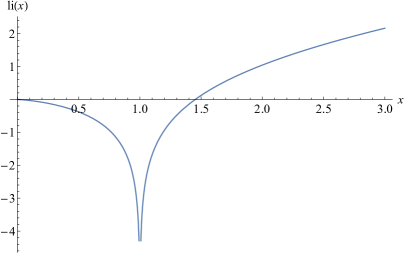
Figure 2: The logarithmic integral function.

The discontinuity of $\psi_{u}$ in $x=1$ introduces a degeneracy in the eigenstates of $\hat{u}$. For each eigenvalue we can choose two independent eigenstates,

$$\psi_{u}^{1}(x)=\left\{\begin{array}[]{l}\frac{1}{\sqrt{8\pi\hbar\left|\ln(\epsilon)\right|}}\exp\left(\frac{iM_{0}}{\hbar}(u-v)\frac{x-\epsilon}{\ln(\epsilon)}\right),\quad x<\epsilon\\ \frac{1}{\sqrt{8\pi\hbar\left|\ln(x)\right|}}\exp\left(\frac{iM_{0}}{\hbar}(u-v)\left[{\rm li}\left(x\right)-{\rm li}\left(\epsilon\right)\right]\right),\quad\epsilon\leq x<1\\ 0,\quad x\geq 1\end{array}\right.$$ (25)

$$\psi_{u}^{2}(x)=\left\{\begin{array}[]{l}0,\quad x\leq 1\\ \frac{1}{\sqrt{8\pi\hbar\left|\ln(x)\right|}}\exp\left(\frac{iM_{0}}{\hbar}(u-v)\left[{\rm li}\left(x\right)-{\rm li}\left(\epsilon\right)\right]\right),\quad x>1\end{array}\right.$$ (26)

which we have chosen as orthonormal. We will adopt the notation $\left|u,J\right\rangle_{\epsilon}$ with $J=1,2$ for these states.

IV.2 Operators associated with the Bogoliubov coefficients and their expectation values

On the previously described quantum space-time we will study Hawking radiation associated with a scalar field. We will assume that the scalar field sees a superposition of geometries corresponding to different masses of the black hole. Therefore, to measure observables associated with the field one needs to take their expectation value with respect to the wave-function of the black hole. In this subsection we will apply these ideas to the computation of the Bogoliubov coefficients and in the next we will extend it to compute the density matrix. We will go from the usual Bogoliubov coefficient $\beta_{\omega\omega^{\prime}}$ to the operator $\hat{\beta}_{\omega\omega^{\prime}}$. We will then compute its expectation value on a wave-function packet associated to the black hole and centered on the classical values $\overline{M}$ and $\overline{v}_{0}$. We start with the expression (3) and promote it to a well defined operator

$$\hat{\beta}_{\omega\omega^{\prime}}=-\frac{1}{2\pi}\sqrt{\frac{\omega^{\prime}}{\omega}}\underset{\epsilon\to 0}{\lim}{\int_{-\infty}^{+\infty}}dv\theta\left(\widehat{v}_{0}-v\widehat{I}\right)e^{-i\omega\hat{u}_{\epsilon}(v)-i\omega^{\prime}v}\theta\left(\widehat{v}_{0}-v\widehat{I}\right).$$ (27)

We then consider a state $\Psi$ associated with the black hole and compute the expectation value,

$$\left\langle\hat{\beta}\right\rangle_{\omega\omega^{\prime}}=-\frac{1}{2\pi}\sqrt{\frac{\omega^{\prime}}{\omega}}\underset{\epsilon\to 0}{\lim}\left\langle\Psi\right|{\int_{-\infty}^{+\infty}}dv{\int_{-\infty}^{+\infty}}dv_{0}\left|v_{0}\right\rangle\left\langle v_{0}\right|\theta\left(\widehat{v}_{0}-v\widehat{I}\right)e^{-i\omega\hat{u}_{\epsilon}(v)-i\omega^{\prime}v}\times$$

$$\times\underset{J=1,2}{\sum}{\int_{-\infty}^{+\infty}}du\left|u,J\right\rangle_{\epsilon\epsilon}\left\langle u,J\right|{\int_{-\infty}^{+\infty}}dv^{\prime}_{0}\left|v^{\prime}_{0}\right\rangle\left\langle v^{\prime}_{0}\right|\theta\left(\widehat{v}_{0}-v\widehat{I}\right)\left|\Psi\right\rangle,$$

where we have introduced bases of eigenstates of $\hat{v}_{0}$ and $\hat{u}$.

Given,

$$\left\langle\hat{\beta}\right\rangle_{\omega\omega^{\prime}}=-\frac{1}{2\pi}\sqrt{\frac{\omega^{\prime}}{\omega}}\underset{\epsilon\to 0}{\lim}{\int_{-\infty}^{\infty}\int_{-\infty}^{\infty}\int_{-\infty}^{\infty}\int_{-\infty}^{\infty}}dvdv_{0}dv^{\prime}_{0}du\Psi^{*}(v_{0})\Psi(v^{\prime}_{0})\theta\left(v_{0}-v\right)\theta\left(v^{\prime}_{0}-v\right)\times$$

$$\times e^{-i\omega u-i\omega^{\prime}v}\underset{J=1,2}{\sum}\psi_{u,J}(v_{0})\psi_{u,J}^{*}(v^{\prime}_{0}),$$

and changing variables $x_{1}=\frac{v_{0}-v}{4M_{0}}$ and $x_{2}=\frac{v^{\prime}_{0}-v}{4M_{0}}$ we get

$$\left\langle\hat{\beta}\right\rangle_{\omega\omega^{\prime}}=-\frac{\left(4M_{0}\right)^{2}}{2\pi}\sqrt{\frac{\omega^{\prime}}{\omega}}\underset{\epsilon\to 0}{\lim}{\int_{-\infty}^{\infty}}dve^{-i\omega^{\prime}v}{\int_{0}^{\infty}\int_{0}^{\infty}}dx_{1}dx_{2}\Psi^{*}(4M_{0}x_{1}+v)\times$$

$$\times\Psi(4M_{0}x_{2}+v){\int_{-\infty}^{+\infty}}due^{-i\omega u}\underset{J=1,2}{\sum}\psi_{u}^{J}(x_{1})\psi_{u}^{J*}(x_{2}).$$ (28)

The definition of the eigenstates $\psi_{u}^{I}$ reduces the integral in ${\int_{0}^{\infty}\int_{0}^{\infty}}dx_{1}dx_{2}$ to

$${\int_{0}^{\epsilon}\int_{0}^{\epsilon}}dx_{1}dx_{2}+{\int_{0}^{\epsilon}}{\int_{\epsilon}^{1}}dx_{1}dx_{2}+{\int_{\epsilon}^{1}}{\int_{0}^{\epsilon}}dx_{1}dx_{2}+{\int_{\epsilon}^{1}\int_{\epsilon}^{1}}dx_{1}dx_{2}+{\int_{1}^{\infty}\int_{1}^{\infty}}dx_{1}dx_{2}.$$

In the appendix we show that the first 3 integrals do not contribute in the limit $\epsilon\to 0$. Therefore the calculation reduces to,

$$\left\langle\hat{\beta}\right\rangle_{\omega\omega^{\prime}}=-\frac{\left(4M_{0}\right)^{2}}{2\pi 8\pi\hbar}\sqrt{\frac{\omega^{\prime}}{\omega}}\underset{\epsilon\to 0}{\lim}{\int_{-\infty}^{\infty}}dve^{-i\omega^{\prime}v}\left({\int_{\epsilon}^{1}\int_{\epsilon}^{1}}dx_{1}dx_{2}+{\int_{1}^{\infty}\int_{1}^{\infty}}dx_{1}dx_{2}\right)\Psi^{*}(4M_{0}x_{1}+v)\times$$

$$\times\Psi(4M_{0}x_{2}+v){\int_{-\infty}^{\infty}}due^{-i\omega u}\frac{1}{\sqrt{\left|\ln(x_{2})\right|\left|\ln(x_{1})\right|}}\exp\left(\frac{iM_{0}}{\hbar}(u-v)\left[{\rm li}(x_{1})-{\rm li}(x_{2})\right]\right).$$

Computing the integral in $u$ we get,

$$\left\langle\hat{\beta}\right\rangle_{\omega\omega^{\prime}}=-\frac{\left(4M_{0}\right)^{2}}{2\pi 8\pi\hbar}\sqrt{\frac{\omega^{\prime}}{\omega}}\underset{\epsilon\to 0}{\lim}{\int_{-\infty}^{\infty}}dv\,e^{-i\omega^{\prime}v}\left({\int_{\epsilon}^{1}\int_{\epsilon}^{1}}dx_{1}dx_{2}+{\int_{1}^{\infty}\int_{1}^{\infty}}dx_{1}dx_{2}\right)\Psi^{*}(4M_{0}x_{1}+v)\times$$

$$\times\Psi(4M_{0}x_{2}+v)\frac{2\pi\delta\left(\omega-\frac{M_{0}}{\hbar}\left[{\rm li}(x_{1})-{\rm li}(x_{2})\right]\right)}{\sqrt{\left|\ln(x_{2})\right|\left|\ln(x_{1})\right|}}e^{-i\omega v}.$$

Since ${\rm li}$ is invertible in $\left(0,1\right)$ and in $\left(1,+\infty\right)$ we can then integrate in $x_{2}$ to get

$$\left\langle\hat{\beta}\right\rangle_{\omega\omega^{\prime}}=-\frac{2M_{0}}{\pi}\sqrt{\frac{\omega^{\prime}}{\omega}}{\int_{-\infty}^{\infty}}dve^{-i\omega^{\prime}v}\left({\int_{0}^{1}}dx_{1}+{\int_{1}^{\infty}}dx_{1}\right)\times$$

$$\times\Psi^{*}(4M_{0}x_{1}+v)\Psi(4M_{0}x_{2}\left(x_{1}\right)+v)\sqrt{\frac{\left|\ln(x_{2})\right|}{\left|\ln(x_{1})\right|}}e^{-i\omega v},$$

where $x_{2}\left(x_{1}\right)={\rm li}^{-1}\left[{\rm li}\left(x_{1}\right)-\frac{\omega\hbar}{M_{0}}\right]$ and we have used that $\partial_{t}{\rm li}\left(t\right)=\frac{1}{\left|\ln(t)\right|}$. We redefine $x=x_{1}$ and

$$\bar{x}_{\omega}(x)={\rm li}^{-1}\left[{\rm li}\left(x\right)-\frac{\omega\hbar}{M_{0}}\right].$$ (29)

Therefore,

$$\left\langle\hat{\beta}\right\rangle_{\omega\omega^{\prime}}=-\frac{2M_{0}}{\pi}\sqrt{\frac{\omega^{\prime}}{\omega}}{\int_{0}^{\infty}}dx\sqrt{\frac{\left|\ln(\bar{x}_{\omega}\left(x\right))\right|}{\left|\ln(x)\right|}}{\int_{-\infty}^{\infty}}dve^{-i\left[\omega+\omega^{\prime}\right]v}\Psi^{*}(4M_{0}x+v)\Psi(4M_{0}\bar{x}_{\omega}\left(x\right)+v),$$

where we have inverted the order of the integrals for convenience of subsequent calculations. Finally, the change of variable $s\equiv v+2M_{0}\left[x+\bar{x}_{\omega}(x)\right]$ gives us

$$\left\langle\hat{\beta}\right\rangle_{\omega\omega^{\prime}}=-\frac{2M_{0}}{\pi}\sqrt{\frac{\omega^{\prime}}{\omega}}{\int_{0}^{\infty}}dx\sqrt{\frac{\left|\ln(\bar{x}_{\omega}\left(x\right))\right|}{\left|\ln(x)\right|}}e^{i2M_{0}\left[\omega+\omega^{\prime}\right]\left[x+\bar{x}_{\omega}(x)\right]}{\int_{-\infty}^{\infty}}dse^{-i\left[\omega+\omega^{\prime}\right]s}\Psi^{*}(s+2M_{0}\Delta_{\omega}(x))\Psi(s-2M_{0}\Delta_{\omega}(x)),$$

with $\Delta_{\omega}(x)\equiv x-\bar{x}_{\omega}(x)$. To better connect this expression with the classical case we can make the general assumption that the wave-packet $\Psi$ of the shell is centered in time $\bar{v}_{0}$ and mass $\bar{M}$. We define $\Phi$ such that

$$\Psi(v_{0})\equiv\Phi(v_{0}-\bar{v}_{0})e^{-i\bar{M}\frac{v_{0}-\bar{v}_{0}}{\hbar}}.$$ (30)

Now

$$\left\langle\hat{\beta}\right\rangle_{\omega\omega^{\prime}}=-\frac{2M_{0}e^{-i\left[\omega+\omega^{\prime}\right]\bar{v}_{0}}}{\pi}\sqrt{\frac{\omega^{\prime}}{\omega}}{\int_{0}^{\infty}}dx\sqrt{\frac{\left|\ln(\bar{x}_{\omega}\left(x\right))\right|}{\left|\ln(x)\right|}}e^{i4M_{0}\left[\omega+\omega^{\prime}\right]x}e^{-i2M_{0}\left[\omega+\omega^{\prime}\right]\Delta_{\omega}(x)}e^{i\frac{4\bar{M}M_{0}}{\hbar}\Delta_{\omega}(x)}\times$$

$$\times{\int_{-\infty}^{\infty}}dse^{-i\left[\omega+\omega^{\prime}\right]s}\Phi^{*}(s+2M_{0}\Delta_{\omega}(x))\Phi(s-2M_{0}\Delta_{\omega}(x)).$$ (31)

As a possible wave-function for the black hole we consider a Gaussian centered in $\bar{v}_{0}$ and $\bar{M}_{0}$ whose $v_{0}$ representation is

$$\Psi_{b}\left(v_{0}\right)=\frac{1}{\left(\pi\sigma^{2}\right)^{\frac{1}{4}}}e^{-\frac{\left(v_{0}-\bar{v}_{0}\right)^{2}}{2\sigma^{2}}}e^{-i\bar{M}\frac{v_{0}-\bar{v_{0}}}{\hbar}}.$$ (32)

Using this wave-function we get

$$\left\langle\hat{\beta}\right\rangle_{\omega\omega^{\prime}}=-\frac{2M_{0}e^{-i\left[\omega+\omega^{\prime}\right]\bar{v}_{0}}}{\pi}\sqrt{\frac{\omega^{\prime}}{\omega}}{\int_{0}^{\infty}}dx\sqrt{\frac{\left|\ln(\bar{x}_{\omega}\left(x\right))\right|}{\left|\ln(x)\right|}}e^{i4M_{0}\left[\omega+\omega^{\prime}\right]x}e^{-i2M_{0}\left[\omega+\omega^{\prime}\right]\Delta_{\omega}(x)}e^{i\frac{4\bar{M}M_{0}}{\hbar}\Delta_{\omega}(x)}\times$$

$$\times\frac{1}{\left(\pi\sigma^{2}\right)^{\frac{1}{2}}}e^{-\frac{4M_{0}^{2}\Delta_{\omega}(x)^{2}}{\sigma^{2}}}{\int_{-\infty}^{\infty}}dse^{-i\left[\omega+\omega^{\prime}\right]s}e^{-\frac{s^{2}}{\sigma^{2}}}.$$

Computing the Gaussian integral

$$\left\langle\hat{\beta}\right\rangle_{\omega\omega^{\prime}}=-\frac{2M_{0}}{\pi}\sqrt{\frac{\omega^{\prime}}{\omega}}e^{-i\left[\omega+\omega^{\prime}\right]\bar{v}_{0}}e^{-\left[\omega+\omega^{\prime}\right]^{2}\frac{\sigma^{2}}{4}}{\int_{0}^{\infty}}dx\sqrt{\frac{\left|\ln(\bar{x}_{\omega}\left(x\right))\right|}{\left|\ln(x)\right|}}\times$$

$$\times e^{i4M_{0}\left[\omega+\omega^{\prime}\right]x}e^{i\frac{4\bar{M}M_{0}}{\hbar}\Delta_{\omega}(x)}e^{-\frac{4M_{0}^{2}}{\sigma^{2}}\Delta_{\omega}(x)^{2}}e^{-i2M_{0}\left[\omega+\omega^{\prime}\right]\Delta_{\omega}(x)}.$$ (33)

To check the consistency of this result we can get the classical limit by taking $\hbar$ to zero and the width of the packet in both canonical variables to zero as well,

$$\hbar\to 0,\ \sigma\to 0\quad\text{with }\quad\frac{\hbar}{\sigma}\to 0.$$ (34)

In that limit $\bar{x}_{\omega}(x)={\rm li}^{-1}\left[{\rm li}(x)-\frac{\omega\hbar}{M_{0}}\right]\to x$ and $\frac{\Delta_{\omega}(x)}{\hbar}\to\frac{\omega}{M_{0}}\ln(x)$. Therefore,

$$\left\langle\hat{\beta}\right\rangle_{\omega\omega^{\prime}}\underset{\hbar\to 0}{\longrightarrow}-\frac{4M_{0}}{2\pi}\sqrt{\frac{\omega^{\prime}}{\omega}}e^{-i\left[\omega+\omega^{\prime}\right]\bar{v_{0}}}{\int_{0}^{\infty}}dxe^{4M_{0}i\left[\omega+\omega^{\prime}\right]x}e^{i4\bar{M}\omega\ln(x)}=\beta_{\omega\omega^{\prime}}$$

and we recover the classical expression (12).

IV.3 Corrections to Hawking radiation: a first approach

In the previous subsection we obtained the Bogoliubov coefficients in the full quantum treatment and showed that we recover the classical result in the classical limit (34). Here we would like to study deviations from the classical behaviour. For it, we will use the expectation values derived in the previous section. This is only a first approximation since the correct expression involves the expectation value of products of the operators associated with the Bogoliubov coefficients. We will later see that this implies an important difference and an interesting example of how the quantum fluctuations may be determinant and lead to significant departures from the mean field approach.

We will consider the example of a Gaussian wave-packet for the wave-function of the shell and arrive to some general conclusions. Then, to maintain tractable expressions, we will restrict attention to “extreme” cases of the latter: one with the Gaussian very peaked in mass (with large dispersion in $v_{0}$) and the other with the Gaussian very peaked in $v_{0}$ (with large dispersion in the mass).

Let us start with some general considerations about the expectation value of the operator associated with the Bogoliubov coefficients. Expression (33) has several differences with the classical limit (12), especially in the dependence with the frequency $\omega^{\prime}$. Lets focus in the integrand

$$\sqrt{\frac{\left|\ln(\bar{x}_{\omega}\left(x\right))\right|}{\left|\ln(x)\right|}}e^{i4M_{0}\left[\omega+\omega^{\prime}\right]x}e^{i\frac{4\bar{M}M_{0}}{\hbar}\Delta_{\omega}(x)}e^{-\frac{4M_{0}^{2}}{\sigma^{2}}\Delta_{\omega}(x)^{2}}e^{-i2M_{0}\left[\omega+\omega^{\prime}\right]\Delta_{\omega}(x)}.$$

Taking into account that

$$\Delta_{\omega}(x)\underset{x\to 0}{\longrightarrow}{\rm li}^{-1}\left(-\frac{\hbar\omega}{M_{0}}\right)$$

$$\Delta_{\omega}(x)\underset{x\to+\infty}{\sim}\frac{\hbar\omega}{M_{0}}\ln(x),$$

and remembering that

$$\bar{x}_{\omega}(x)={\rm li}^{-1}\left({\rm li}(x)-\frac{\hbar\omega}{M_{0}}\right),$$

we see it vanishes when $x\to 0$, also $\sqrt{\frac{\left|\ln(\bar{x}_{\omega}\left(x\right))\right|}{\left|\ln(x)\right|}}$ is bounded by $1$ and finally

$$e^{-\frac{4M_{0}^{2}}{\sigma^{2}}\Delta_{\omega}(x)^{2}}\underset{x\to+\infty}{\sim}e^{-\frac{4\hbar^{2}}{\sigma^{2}}\ln(x)^{2}}.$$

Therefore the integral has a bound (independent of $\omega^{\prime}$) given by

$${\int_{0}^{\infty}}dxe^{-\frac{4M_{0}^{2}}{\sigma^{2}}\Delta_{\omega}(x)^{2}}.$$

This fact, together with the exponential factor $e^{-\left[\omega+\omega^{\prime}\right]^{2}\frac{\sigma^{2}}{4}}$ outside the integral, ensures exponential suppression of large $\omega^{\prime}$ contributions. The integral also lacks the $\frac{1}{\omega^{\prime}+\omega}$ dependence that the classical expression has since setting $\omega^{\prime}=\omega=0$ inside the integral still gives us a finite result.

One quantity that is extremely sensitive to these differences is the total number of emitted particles per unit frequency. If we compute it using the expectation value of the Bogoliubov coefficients it will be given by

$$\left\langle N_{\omega}^{AQS}\right\rangle={\int_{0}^{\infty}}d\omega^{\prime}\left\langle\hat{\beta}\right\rangle_{\omega\omega^{\prime}}\left\langle\hat{\beta}\right\rangle_{\omega\omega^{\prime}}^{*}$$ (35)

where the superscript “AQS” stands for Approximate Quantum Shell. The reason to call it approximate is that the correct way to compute it would be with the expectation value of the product of Bogoliubov coefficients instead of the product of expectation values. We will address this important issue in the next section, but for now we will assume that fluctuations are small and this is a good approximation.

Given the previous general remarks about Bogoliubov coefficients we conclude $\left\langle N_{\omega}^{AQS}\right\rangle$ is not divergent as in the classical expression (14) but finite which is a big departure from eternal Hawking radiation.

A more explicit analysis can be performed with a state that is squeezed with large dispersion in the position of the shell and very peaked in the mass. Specifically, we will consider the case where the shell is in a Gaussian (32) squeezed state with large dispersion in $v_{0}$ and small dispersion in $M$. The leading quantum correction for such states is obtained by taking the limit $\hbar\to 0$ with

$$\Delta v_{0}=\sigma=\text{constant}=Z\ell_{\text{Planck}}\;,\;Z\gg 1\,;\quad\Delta M=\hbar/\sigma.$$ (36)

Even though this limit is different from the one we took following (33) it has similarities with it. The terms inside the integral go to their classical values but the external factor involving $\sigma$ now remains. One then finds that (33) goes to:

$$\left\langle\hat{\beta}\right\rangle_{\omega\omega^{\prime}}\to e^{-\left[\omega+\omega^{\prime}\right]^{2}\frac{\sigma^{2}}{4}}\beta_{\omega\omega^{\prime}}.$$ (37)

The deviation from the classical Bogoliubov coefficients is only through a multiplicative factor that disappears in the classical limit where $\sigma\to 0$. For non-zero $\sigma$ the factor suppresses frequencies greater than $1/\sigma$. This produces important corrections to the calculation of Hawking radiation as we already mentioned. However this calculation is based in an approximation in which we computed the square of the expectation value of the Bogoliubov coefficients instead of the expectation value of the square. It turns out this approximation breaks down. We present detailed calculations in the appendix. Here we just outline the calculation.

Estimating the expectation value of the number operator using expression (37) we get,

$$\left\langle N_{\omega}^{AQS}\right\rangle={\int_{0}^{\infty}}d\omega^{\prime}\left\langle\hat{\beta}\right\rangle_{\omega\omega^{\prime}}\left\langle\hat{\beta}\right\rangle_{\omega\omega^{\prime}}^{*}=\frac{1}{4\pi^{2}}\frac{1}{\omega}\left|\Gamma(1+4\bar{M}\omega i)\right|^{2}e^{-4\pi\bar{M}\omega}{\int_{0}^{\infty}}d\omega^{\prime}\frac{\omega^{\prime}e^{-\left[\omega+\omega^{\prime}\right]^{2}\frac{\sigma^{2}}{2}}}{\left(\omega^{\prime}+\omega\right)^{2}}=$$

$$=\frac{1}{e^{8\bar{M}\pi\omega}-1}\frac{2\bar{M}}{\pi}{\int_{0}^{\infty}}d\omega^{\prime}\frac{\omega^{\prime}e^{-\left[\omega+\omega^{\prime}\right]^{2}\frac{\sigma^{2}}{2}}}{\left(\omega^{\prime}+\omega\right)^{2}}.$$ (38)

This expression has the same pre-factor Hawking radiation has but with $\bar{M}$ in the role of mass. However, unlike (14) this is a finite expression for all $\omega\neq 0$ and has a logarithmic divergence when $\omega\to 0$. Furthermore, it has a $\exp(-\frac{\omega^{2}\sigma^{2}}{2})$ dependence when $\omega\to+\infty$ instead of the usual $\exp(-8\bar{M}\pi\omega)$ for Hawking radiation.

Since we are interested in the behaviour of the Hawking radiation as a function of time it is convenient to introduce wave packets as we considered before and therefore to compute the number of particles at time $u_{n}$ around $\omega_{j}$ given by,

$$\langle N_{\omega_{j}}^{AQS}\rangle=\frac{1}{\epsilon}{\int_{j\epsilon}^{\left(j+1\right)\epsilon}\int_{j\epsilon}^{\left(j+1\right)\epsilon}}d\omega_{1}d\omega_{2}e^{-u_{n}\Delta\omega i}\left\langle\rho^{AQS}_{\omega_{1},\omega_{2}}\right\rangle.$$

Using the results in appendix 2 it can be computed explicitly, yielding,

$$\langle N_{\omega_{j}}^{AQS}\rangle=\frac{\bar{M}\epsilon}{\pi}\frac{1}{e^{8\bar{M}\pi\omega_{j}}-1}{\int_{1}^{\infty}}dy\frac{e^{-\frac{\omega_{j}^{2}\sigma^{2}}{2}y}}{y}\left\{\frac{\sin\left[\frac{\epsilon}{2}\left(\alpha-2\bar{M}\ln\left(y\right)\right)\right]}{\frac{\epsilon}{2}\left(\alpha-2\bar{M}\ln\left(y\right)\right)}\right\}^{2}.$$

Where $\alpha$ is the same quantity defined in equation (17) with $M$ and $v_{0}$ replaced by their respective expectation values in the Gaussian state given above. The presence of the factor $\sin^{2}(a)/a^{2}$ and the decreasing exponential imply that the integral decreases when $\alpha$ grows and also drastically decreases when $\alpha<0$. The latter is a result we already knew from the classical case, but the former is a result of the quantum nature of the black hole since it is not present if $\sigma=0$. Figure (3) shows the departure from the classical result that appears when one computes the frequency distribution starting from $\left\langle\hat{\beta}\right\rangle$. We can estimate the time of emission for each frequency using both extremes. In the appendix we also show that the features are robust with respect to the choice of the quantum state by considering squeezed states with large dispersion in the mass, which is the opposite of the choice we considered here. However, as we shall see in the next section, the decrease in emission for late time is an artifact of the approximation considered that neglects the fluctuations of the number of particles.

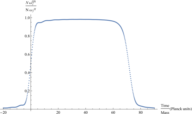
Figure 3: This plot shows the departure from the classical result of $N^{AQS}_{\omega_{j}}/N^{H}_{\omega_{j}}$. We have considered $\omega_{j}$ corresponding to the $\lambda$ of maximum emission ($\lambda_{m}\sim 16R_{s}$), the frequency interval $\epsilon=c/R_{s}$ and the shell’s position uncertainty $\sigma=5R_{s}\times 10^{-38}$ ($\sim 3l_{P}$ for $R_{s}=1km$). Note that the time step is $2\pi/\epsilon$.

V Computing the expectation value of the density matrix in the complete quantum treatment

In this section we will obtain an exact expression for the expectation value of the density matrix with the same technique used to compute the expectation value of Bogoliubov coefficients. From its diagonal terms we can compute the number of particles produced as a function of frequency.

From expression (27) for the operator associated to a Bogoliubov coefficient we can compute the expectation value of the density matrix as

$$\left\langle\rho_{\omega_{1}\omega_{2}}^{QS}\right\rangle=\int_{0}^{\infty}d\omega^{\prime}\left\langle\hat{\beta}_{\omega_{1}\omega^{\prime}}\hat{\beta}_{\omega_{2}\omega^{\prime}}^{*}\right\rangle.$$

where $QS$ stands for quantum shell. The full expression is

$$\left\langle\rho_{\omega_{1}\omega_{2}}^{QS}\right\rangle=\frac{1}{(2\pi)^{2}}\int_{0}^{\infty}d\omega^{\prime}\frac{\omega^{\prime}}{\sqrt{\omega_{1}\omega_{2}}}\left\langle\Psi\right|{{\int\int}_{-\infty}^{+\infty}}dvdv^{\prime}{\int_{-\infty}^{+\infty}}dv_{0}\left|v_{0}\right\rangle\left\langle v_{0}\right|\theta\left(\widehat{v}_{0}-v\widehat{I}\right)e^{-i\omega_{1}\hat{u}(v)-i\omega^{\prime}v}\times$$

$$\times\underset{J=1,2}{\sum}{\int_{-\infty}^{+\infty}}du\left|u,J\right\rangle\left\langle u,J\right|{\int_{-\infty}^{+\infty}}dv^{\prime\prime}_{0}\left|v^{\prime\prime}_{0}\right\rangle\left\langle v^{\prime\prime}_{0}\right|\theta\left(\widehat{v}_{0}-v\widehat{I}\right){\int_{-\infty}^{+\infty}}dv^{\prime\prime\prime}_{0}\left|v^{\prime\prime\prime}_{0}\right\rangle\left\langle v^{\prime\prime\prime}_{0}\right|\theta\left(\widehat{v}_{0}-v^{\prime}\widehat{I}\right)\times$$

$$\times\underset{L=1,2}{\sum}{\int_{-\infty}^{+\infty}}du^{\prime}\left|u^{\prime},L\right\rangle\left\langle u^{\prime},L\right|e^{i\omega_{2}\hat{u^{\prime}}(v^{\prime})+i\omega^{\prime}v^{\prime}}{\int_{-\infty}^{+\infty}}dv^{\prime}_{0}\left|v^{\prime}_{0}\right\rangle\left\langle v^{\prime}_{0}\right|\theta\left(\widehat{v}_{0}-v^{\prime}\widehat{I}\right)\left|\Psi\right\rangle.$$

Here we have considered bases of eigenstates of $\hat{v}_{0}$ and $\hat{u}$ and we have omitted the $\epsilon$ dependence in $\hat{u}$ eigenstates. Identical arguments as the ones used in the appendix allow us to do so. Simplifying the expression we get

$$\left\langle\rho_{\omega_{1}\omega_{2}}^{QS}\right\rangle=\frac{1}{(2\pi)^{2}}\int_{0}^{\infty}d\omega^{\prime}\frac{\omega^{\prime}}{\sqrt{\omega_{1}\omega_{2}}}{{\int}_{-\infty}^{+\infty}}dvdv^{\prime}dv_{0}dv^{\prime}_{0}dv^{\prime\prime}_{0}dv^{\prime\prime\prime}_{0}\theta\left(v_{0}-v\right)\theta\left(v^{\prime\prime}_{0}-v\right)\theta\left(v^{\prime\prime\prime}_{0}-v^{\prime}\right)\theta\left(v^{\prime}_{0}-v^{\prime}\right)\delta\left(v^{\prime\prime}_{0}-v^{\prime\prime\prime}_{0}\right)\times$$

$$\times{\int}_{-\infty}^{+\infty}dudu^{\prime}e^{-i\omega_{1}u-i\omega^{\prime}v}\underset{J=1,2}{\sum}\psi_{u,J}(v_{0})\psi_{u,J}^{*}(v^{\prime\prime}_{0})e^{i\omega_{2}u^{\prime}+i\omega^{\prime}v^{\prime}}\underset{L=1,2}{\sum}\psi_{u^{\prime},L}(v^{\prime\prime\prime}_{0})\psi_{u^{\prime},L}^{*}(v^{\prime}_{0})\Psi^{*}(v_{0})\Psi(v^{\prime}_{0}),$$

The change of variables $x_{1}=\frac{v_{0}-v}{4M_{0}}$, $x_{2}=\frac{v^{\prime\prime}_{0}-v}{4M_{0}}$, $x_{3}=\frac{v^{\prime\prime\prime}_{0}-v^{\prime}}{4M_{0}}$ y $x_{4}=\frac{v^{\prime}_{0}-v^{\prime}}{4M_{0}}$ take us to

$$\left\langle\rho_{\omega_{1}\omega_{2}}^{QS}\right\rangle=\frac{\left(4M_{0}\right)^{4}}{(2\pi)^{2}}\int_{0}^{\infty}d\omega^{\prime}\frac{\omega^{\prime}}{\sqrt{\omega_{1}\omega_{2}}}{{\int}_{-\infty}^{+\infty}}dvdv^{\prime}{\int}_{0}^{+\infty}dx_{1}dx_{2}dx_{3}dx_{4}\delta\left(4M_{0}\left[x_{2}-x_{3}\right]+v-v^{\prime}\right)\times$$

$$\times{\int}_{-\infty}^{+\infty}dudu^{\prime}e^{-i\omega_{1}u-i\omega^{\prime}v}\underset{J=1,2}{\sum}\psi_{u,J}(x_{1})\psi_{u,J}^{*}(x_{2})e^{i\omega_{2}u^{\prime}+i\omega^{\prime}v^{\prime}}\underset{L=1,2}{\sum}\psi_{u^{\prime},L}(x_{3})\psi_{u^{\prime},L}^{*}(x_{4})\Psi^{*}(4M_{0}x_{1}+v)\Psi(4M_{0}x_{4}+v^{\prime}).$$

Using expressions (25) and (26) for the eigenfunctions of the $\hat{u}$ operator

$$\left\langle\rho_{\omega_{1}\omega_{2}}^{QS}\right\rangle=\frac{\left(4M_{0}\right)^{4}}{(16\pi^{2}\hbar)^{2}}\int_{0}^{\infty}d\omega^{\prime}\frac{\omega^{\prime}}{\sqrt{\omega_{1}\omega_{2}}}{{\int}_{-\infty}^{+\infty}}dvdv^{\prime}{\int}_{0}^{+\infty}dx_{1}dx_{2}{\int}_{0}^{+\infty}dx_{3}dx_{4}\delta\left(4M_{0}\left[x_{2}-x_{3}\right]+v-v^{\prime}\right){\int}_{-\infty}^{+\infty}dudu^{\prime}\times$$

$$\times e^{-i\omega_{1}u-i\omega^{\prime}v}e^{i\omega_{2}u^{\prime}+i\omega^{\prime}v^{\prime}}\frac{\exp\left(\frac{iM_{0}}{\hbar}(u-v)\left[{\rm li}(x_{1})-{\rm li}(x_{2})\right]\right)\exp\left(\frac{iM_{0}}{\hbar}(u^{\prime}-v^{\prime})\left[{\rm li}(x_{3})-{\rm li}(x_{4})\right]\right)}{\sqrt{\left|\ln(x_{1})\right|\left|\ln(x_{2})\right|\left|\ln(x_{3})\right|\left|\ln(x_{4})\right|}}\Psi^{*}(4M_{0}x_{1}+v)\Psi(4M_{0}x_{4}+v^{\prime}).$$

Integrating in $u$ y $u^{\prime}$ we get,

$$\left\langle\rho_{\omega_{1}\omega_{2}}^{QS}\right\rangle=\frac{\left(4M_{0}\right)^{4}}{(8\pi\hbar)^{2}}\int_{0}^{\infty}d\omega^{\prime}\frac{\omega^{\prime}}{\sqrt{\omega_{1}\omega_{2}}}{{\int}_{-\infty}^{+\infty}}dvdv^{\prime}{\int}_{0}^{+\infty}dx_{1}dx_{2}{\int}_{0}^{+\infty}dx_{3}dx_{4}\delta\left(4M_{0}\left[x_{2}-x_{3}\right]+v-v^{\prime}\right)\times$$

$$\times e^{-i\left[\omega^{\prime}+\omega_{1}\right]v}e^{i\left[\omega^{\prime}+\omega_{2}\right]v^{\prime}}\frac{\delta\left(\omega_{1}-\frac{M_{0}}{\hbar}\left[{\rm li}(x_{1})-{\rm li}(x_{2})\right]\right)\delta\left(\omega_{2}+\frac{M_{0}}{\hbar}\left[{\rm li}(x_{3})-{\rm li}(x_{4})\right]\right)}{\sqrt{\left|\ln(x_{1})\right|\left|\ln(x_{2})\right|\left|\ln(x_{3})\right|\left|\ln(x_{4})\right|}}\Psi^{*}(4M_{0}x_{1}+v)\Psi(4M_{0}x_{4}+v^{\prime}).$$

Since ${\rm li}$ is invertible in $\left(0,1\right)$ and in $\left(1,+\infty\right)$ we can integrate in $x_{2}$ and $x_{3}$ to get

$$\left\langle\rho_{\omega_{1}\omega_{2}}^{QS}\right\rangle=\frac{\left(2M_{0}\right)^{2}}{\pi^{2}}\int_{0}^{\infty}d\omega^{\prime}\frac{\omega^{\prime}}{\sqrt{\omega_{1}\omega_{2}}}{{\int}_{-\infty}^{+\infty}}dvdv^{\prime}{\int}_{0}^{+\infty}dx_{1}{\int}_{0}^{+\infty}dx_{4}\delta\left(4M_{0}\left[x_{2}(x_{1})-x_{3}(x_{4})\right]+v-v^{\prime}\right)\times$$

$$\times e^{-i\left[\omega^{\prime}+\omega_{1}\right]v}e^{i\left[\omega^{\prime}+\omega_{2}\right]v^{\prime}}\sqrt{\frac{\left|\ln(x_{2}(x_{1})\right|\left|\ln(x_{3}(x_{4}))\right|}{\left|\ln(x_{1})\right|\left|\ln(x_{4})\right|}}\Psi^{*}(4M_{0}x_{1}+v)\Psi(4M_{0}x_{4}+v^{\prime}),$$

where $x_{2}\left(x_{1}\right)={\rm li}^{-1}\left[{\rm li}\left(x_{1}\right)-\frac{\omega_{1}\hbar}{M_{0}}\right]$, $x_{3}\left(x_{4}\right)={\rm li}^{-1}\left[{\rm li}\left(x_{4}\right)-\frac{\omega_{2}\hbar}{M_{0}}\right]$ and we have used that $\partial_{t}{\rm li}\left(t\right)=\frac{1}{\left|\ln(t)\right|}$. We redefine $x=x_{1}$, $x^{\prime}=x_{4}$ and then

$$\left\langle\rho_{\omega_{1}\omega_{2}}^{QS}\right\rangle=\frac{\left(2M_{0}\right)^{2}}{\pi^{2}}\int_{0}^{\infty}d\omega^{\prime}\frac{\omega^{\prime}}{\sqrt{\omega_{1}\omega_{2}}}{{\int}_{-\infty}^{+\infty}}dvdv^{\prime}{\int}_{0}^{+\infty}dxdx^{\prime}\delta\left(4M_{0}\left[\bar{x}_{\omega_{1}}(x)-\bar{x}_{\omega_{2}}(x^{\prime})\right]+v-v^{\prime}\right)\times$$

$$\times e^{-i\left[\omega^{\prime}+\omega_{1}\right]v}e^{i\left[\omega^{\prime}+\omega_{2}\right]v^{\prime}}\sqrt{\frac{\left|\ln(\bar{x}_{\omega_{1}}(x))\right|\left|\ln(\bar{x}_{\omega_{2}}(x^{\prime}))\right|}{\left|\ln(x)\right|\left|\ln(x^{\prime})\right|}}\Psi^{*}(4M_{0}x+v)\Psi(4M_{0}x^{\prime}+v^{\prime}).$$

Integrating in $v^{\prime}$

$$\left\langle\rho_{\omega_{1}\omega_{2}}^{QS}\right\rangle=\frac{\left(2M_{0}\right)^{2}}{\pi^{2}}\int_{0}^{\infty}d\omega^{\prime}\frac{\omega^{\prime}}{\sqrt{\omega_{1}\omega_{2}}}{\int}_{0}^{+\infty}dxdx^{\prime}e^{-i4M_{0}\left[\omega^{\prime}+\omega_{2}\right]x^{\prime}}e^{i4M_{0}\left[\omega^{\prime}+\omega_{2}\right]x}e^{i4M_{0}\left[\omega^{\prime}+\omega_{2}\right]\Delta_{\omega_{1}\omega_{2}}(x,x^{\prime})}\times$$

$$\times\sqrt{\frac{\left|\ln(\bar{x}_{\omega_{1}}(x))\right|\left|\ln(\bar{x}_{\omega_{2}}(x^{\prime}))\right|}{\left|\ln(x)\right|\left|\ln(x^{\prime})\right|}}{{\int}_{-\infty}^{+\infty}}dve^{-i\left[\omega_{1}-\omega_{2}\right]v}\Psi^{*}(4M_{0}x+v)\Psi(4M_{0}x+v+4M_{0}\Delta_{\omega_{1}\omega_{2}}(x,x^{\prime}))$$

where $\Delta_{\omega_{1}\omega_{2}}(x,x^{\prime})=\Delta_{\omega_{2}}(x^{\prime})-\Delta_{\omega_{1}}(x)$. Now, changing variable $v$ to $s=v+4M_{0}x+2M_{0}\Delta_{\omega_{1}\omega_{2}}(x,x^{\prime})$

$$\left\langle\rho_{\omega_{1}\omega_{2}}^{QS}\right\rangle=\frac{\left(2M_{0}\right)^{2}}{\pi^{2}}\int_{0}^{\infty}d\omega^{\prime}\frac{\omega^{\prime}}{\sqrt{\omega_{1}\omega_{2}}}{\int}_{0}^{+\infty}dxdx^{\prime}e^{-i4M_{0}\left[\omega^{\prime}+\omega_{2}\right]x^{\prime}}e^{i4M_{0}\left[\omega^{\prime}+\omega_{1}\right]x}e^{i4M_{0}\left[\omega^{\prime}+\bar{\omega}\right]\Delta_{\omega_{1}\omega_{2}}(x,x^{\prime})}\times$$

$$\times\sqrt{\frac{\left|\ln(\bar{x}_{\omega_{1}}(x))\right|\left|\ln(\bar{x}_{\omega_{2}}(x^{\prime}))\right|}{\left|\ln(x)\right|\left|\ln(x^{\prime})\right|}}{{\int}_{-\infty}^{+\infty}}dse^{-i\left[\omega_{1}-\omega_{2}\right]s}\Psi^{*}(s-2M_{0}\Delta_{\omega_{1}\omega_{2}}(x,x^{\prime}))\Psi(s+2M_{0}\Delta_{\omega_{1}\omega_{2}}(x,x^{\prime}))$$

where $\bar{\omega}=\frac{\omega_{1}+\omega_{2}}{2}$. Finally, using definition (30) we get

$$\left\langle\rho_{\omega_{1}\omega_{2}}^{QS}\right\rangle=\frac{\left(2M_{0}\right)^{2}e^{-i\left[\omega_{1}-\omega_{2}\right]\bar{v}_{0}}}{\pi^{2}\sqrt{\omega_{1}\omega_{2}}}\int_{0}^{\infty}d\omega^{\prime}\omega^{\prime}{\int}_{0}^{+\infty}dxdx^{\prime}e^{-i4M_{0}\left[\omega^{\prime}+\omega_{2}\right]x^{\prime}}e^{i4M_{0}\left[\omega^{\prime}+\omega_{1}\right]x}e^{i4M_{0}\left[\omega^{\prime}+\bar{\omega}\right]\Delta_{\omega_{1}\omega_{2}}(x,x^{\prime})}\times$$

$$\times e^{-i\frac{4M_{0}\bar{M}}{\hbar}\Delta_{\omega_{1}\omega_{2}}(x,x^{\prime})}\sqrt{\frac{\left|\ln(\bar{x}_{\omega_{1}}(x))\right|\left|\ln(\bar{x}_{\omega_{2}}(x^{\prime}))\right|}{\left|\ln(x)\right|\left|\ln(x^{\prime})\right|}}{{\int}_{-\infty}^{+\infty}}dse^{-i\left[\omega_{1}-\omega_{2}\right]s}\Phi^{*}(s-2M_{0}\Delta_{\omega_{1}\omega_{2}}(x,x^{\prime}))\Phi(s+2M_{0}\Delta_{\omega_{1}\omega_{2}}(x,x^{\prime})).$$ (39)

where $\Delta\omega=\omega_{2}-\omega_{1}$. Taking again the Gaussian wavepacket (32) as an example, we get

$$\left\langle\rho_{\omega_{1}\omega_{2}}^{QS}\right\rangle=\frac{\left(2M_{0}\right)^{2}e^{i\Delta\omega\bar{v}_{0}}e^{-\frac{\Delta\omega^{2}\sigma^{2}}{4}}}{\pi^{2}\sqrt{\omega_{1}\omega_{2}}}\int_{0}^{\infty}d\omega^{\prime}\omega^{\prime}{\int}_{0}^{+\infty}dxdx^{\prime}e^{i4M_{0}\left[\omega^{\prime}+\omega_{1}\right]x}e^{-i4M_{0}\left[\omega^{\prime}+\omega_{2}\right]x^{\prime}}\times$$

$$\times e^{i4M_{0}\left[\omega^{\prime}+\bar{\omega}\right]\Delta_{\omega_{1}\omega_{2}}(x,x^{\prime})}e^{-i\frac{4M_{0}\bar{M}}{\hbar}\Delta_{\omega_{1}\omega_{2}}(x,x^{\prime})}\sqrt{\frac{\left|\ln(\bar{x}_{\omega_{1}}(x))\right|\left|\ln(\bar{x}_{\omega_{2}}(x^{\prime}))\right|}{\left|\ln(x)\right|\left|\ln(x^{\prime})\right|}}e^{-\frac{4M_{0}^{2}\Delta_{\omega_{1}\omega_{2}}(x,x^{\prime})^{2}}{\sigma^{2}}}.$$ (40)

This is the final result for the expectation value of the density matrix in the complete quantum treatment.

From this expression we can compute the classical limit (34). In that limit $\bar{x}_{\omega_{1}}(x)\to x$, $\bar{x}_{\omega_{2}}(x^{\prime})\to x^{\prime}$ and $\frac{\Delta_{\omega_{1}\omega_{2}}(x,x^{\prime})}{\hbar}\to\frac{\omega_{2}\ln(x^{\prime})-\omega_{1}\ln(x)}{M_{0}}$. Therefore,

$$\left\langle\rho_{\omega_{1}\omega_{2}}^{QS}\right\rangle=\frac{\left(2M_{0}\right)^{2}e^{i\Delta\omega\bar{v}_{0}}}{\pi^{2}\sqrt{\omega_{1}\omega_{2}}}\int_{0}^{\infty}d\omega^{\prime}\omega^{\prime}{\int}_{0}^{+\infty}dxe^{i4M_{0}\left[\omega^{\prime}+\omega_{1}\right]x}e^{i4\bar{M}\omega_{1}\ln(x)}{\int}_{0}^{+\infty}dx^{\prime}e^{-i4M_{0}\left[\omega^{\prime}+\omega_{2}\right]x^{\prime}}e^{-i4\bar{M}\omega_{2}\ln(x^{\prime})}$$

which is the classical expression for the density matrix

$$\rho^{CS}_{\omega_{1},\omega_{2}}={\int_{0}^{\infty}}d\omega^{\prime}\beta_{\omega_{1}\omega^{\prime}}\beta_{\omega_{2}\omega^{\prime}}^{*}$$

with $\beta_{\omega\omega^{\prime}}$ given by (12).

We analyze the consequences of these calculations in the next section.

VI Corrections to Hawking radiation due to the quantum background

We have studied the corrections to Hawking radiation using the approximate expression (44) discussed in appendix 2. Now we can do the same calculation from the exact expression (40). As in the previous section we begin with some general remarks about the result for a Gaussian state and then explore the same squeezed states we considered before.

Unlike the density matrix constructed from (33), expression (40) has a double integral that can not be separated in $x$ and $x^{\prime}$ variables. But the most significant differences are the missing $\omega^{\prime}$ dependence in the exponential

$$e^{-\frac{\Delta\omega^{2}\sigma^{2}}{4}},$$

and the exponential inside the double integral

$$e^{-\frac{4M_{0}^{2}\left[\Delta_{\omega_{1}\omega_{2}}(x,x^{\prime})\right]^{2}}{\sigma^{2}}}.$$

The first point significantly changes the $\omega^{\prime}$ integral. The second expression does not make the integrand fall rapidly when $x,x^{\prime}\to+\infty$ because the exponential remains constant in the directions give by the equation

$$\Delta_{\omega_{1}\omega_{2}}(x,x^{\prime})=\Delta_{\omega_{2}}(x^{\prime})-\Delta_{\omega_{1}}(x)={\rm const.}$$

As we will see in better detail with the following examples, the consequence of the above remarks are that radiation does not end at a finite time as predicted by evaluations of the expectation value of Bogoliubov coefficients. However, the significant difference between $\left\langle N^{QS}_{\omega}\right\rangle$ and $\left\langle N^{AQS}_{\omega}\right\rangle$ is also generically associated with the appearance of fluctuations in the Bogoliubov coefficients at finite time. We will see that may leads to new correlations in the Hawking radiation that are not present in the classical calculation.

VI.1 States peaked in the mass recover the classical results

Let us consider first the case of a squeezed state with large dispersion in the position of the shell. Taking the limit (36),

$$\left\langle\rho_{\omega_{1}\omega_{2}}^{QS}\right\rangle\to e^{-\frac{\Delta\omega^{2}\sigma^{2}}{4}}\left\langle\rho_{\omega_{1}\omega_{2}}^{CS}\right\rangle.$$ (41)

It is clear that there are no corrections to the total number of particles $\left\langle N^{QS}_{\omega}\right\rangle=\left\langle\rho_{\omega\omega}^{QS}\right\rangle$ since the exponential factor is one if $\omega_{1}=\omega_{2}$. Also, for late times $\left\langle\rho_{\omega_{1}\omega_{2}}^{CS}\right\rangle$ is diagonal so the are no non-vanishing correlations for different frequencies. We therefore recover the classical results in their entirety for the particular case of squeezed states we consider that are highly peaked in the mass and with large dispersion in the position of the shell.

VI.2 States with dispersion in the mass

To illustrate this point let us consider now a squeezed state with large dispersion in the mass of the shell. To compare with the previous result let us compute the number of particles taking the limit (47). We get,

$$\left\langle N_{\omega}^{QS}\right\rangle=\left\langle\rho_{\omega\omega}^{QS}\right\rangle\to\frac{\left(2M_{0}\right)^{2}}{\pi^{2}\omega}\int_{0}^{\infty}d\omega^{\prime}\omega^{\prime}{\int}_{0}^{+\infty}dxdx^{\prime}e^{-\epsilon\left(x+x^{\prime}\right)}e^{-i4M_{0}\left[\omega^{\prime}+\omega\right]\left(x^{\prime}-x\right)}e^{-i4\bar{M}\omega\ln\left(\frac{x^{\prime}}{x}\right)}e^{-4\Delta M^{2}\omega^{2}\ln\left(\frac{x^{\prime}}{x}\right)^{2}}$$ (42)

where we introduced the same $\epsilon$ regulator used for the integration of Bogoliubov coefficients. The change of variables $x=r\cos(\theta)$, $x^{\prime}=r\sin(\theta)$ allow us to compute the double integral as

$$\int_{0}^{\pi/2}d\theta\int_{0}^{+\infty}rdre^{-\epsilon r\left[\sin(\theta)+\cos(\theta)\right]}e^{-i4M_{0}\left[\omega^{\prime}+\omega\right]r\left[\sin(\theta)-cos(\theta)\right]}e^{-i4\bar{M}\omega\ln\left[\tan(\theta)\right]}e^{-4\Delta M^{2}\omega^{2}\ln\left[\tan(\theta)\right]^{2}}.$$

The $r$ integral can be computed, leading to,

$$-\frac{1}{\left[\omega^{\prime}+\omega\right]^{2}(4M_{0})^{2}}\underset{\epsilon\to 0}{\lim}\int_{0}^{\pi/2}d\theta\frac{e^{-i4\bar{M}\omega\ln\left[\tan(\theta)\right]}e^{-4\Delta M^{2}\omega^{2}\ln\left[\tan(\theta)\right]^{2}}}{\left[\frac{\tan(\theta)-1}{\tan(\theta)+1}-i\epsilon\right]^{2}}\frac{1+\tan(\theta)^{2}}{\left[1+\tan(\theta)\right]^{2}},$$

where we have redefined $\epsilon$ conveniently. A final change of variable $y=\ln\left[\tan(\theta)\right]$ turns the integral into

$$-\frac{1}{\left[\omega^{\prime}+\omega\right]^{2}(4M_{0})^{2}}\underset{\epsilon\to 0}{\lim}\int_{-\infty}^{+\infty}dy\frac{1}{2\cosh(y/2)}\frac{e^{-i4\bar{M}\omega y}e^{-4\Delta M^{2}\omega^{2}y^{2}}}{\left[\tanh(y/2)-i\epsilon\right]^{2}}.$$

This expression can be rewritten as

$$-\frac{1}{4\left[\omega^{\prime}+\omega\right]^{2}(4M_{0})^{2}}\left[\underset{\epsilon\to 0}{\lim}\int_{-\infty}^{+\infty}dy\frac{1}{\cosh^{2}(y/2)}\frac{e^{-i4\bar{M}\omega y}}{\left[\tanh(y/2)-i\epsilon\right]^{2}}-\int_{-\infty}^{+\infty}dye^{-i4\bar{M}\omega y}\frac{1-e^{-4\Delta M^{2}\omega^{2}y^{2}}}{\sinh^{2}(y/2)}\right].$$

Now the first integral can be computed by contour integration to obtain the classical result (14) with the expectation value $\bar{M}$ in the role of mass,

$$\underset{\epsilon\to 0}{\lim}\int_{-\infty}^{+\infty}dy\frac{1}{\cosh^{2}(y/2)}\frac{e^{-i4\bar{M}\omega y}}{\left[\tanh(y/2)-i\epsilon\right]^{2}}=\frac{-32\bar{M}\omega\pi}{e^{8\bar{M}\omega\pi}-1}$$

The second term,

$$f(\bar{M},\omega,\Delta M)\equiv\int_{-\infty}^{+\infty}dye^{-i4\bar{M}\omega y}\frac{1-e^{-4\Delta M^{2}\omega^{2}y^{2}}}{\sinh^{2}(y/2)}$$

is a finite correction which vanishes in the classical limit. Regarding the dependence in $\omega$, unlike the leading term it vanishes for $\omega\to 0$ and also as the Fourier transform of a smooth and rapidly falling function it falls rapidly with $\omega\to+\infty$. Finally,

$$\left\langle N_{\omega}^{QS}\right\rangle=\left[\frac{1}{e^{8\bar{M}\omega\pi}-1}+\frac{f(\bar{M},\omega,\Delta M)}{32\pi\omega\bar{M}}\right]\frac{4\bar{M}}{2\pi}\int_{0}^{\infty}d\omega^{\prime}\frac{\omega^{\prime}}{\left[\omega^{\prime}+\omega\right]^{2}}.$$

This expression is clearly divergent, with the same divergent integral that appears in the classical case but with a small departure from thermality given by $f$. It could be made finite considering packets as we did before. Notice that the expression has the thermal spectrum plus a term that only vanishes when there are no fluctuations in the mass. The extra term essentially depends on the Fourier transform of the initial state of the shell and suggests that the complete information of the initial state could be retrieved from the radiation. Recall that in order to recover finite results one needs to compute the number expectation value for wave packets localized in time and frequency. We are therefore led to an expression that departs more and more from ordinary Hawking radiation when the uncertainty in the mass increases.

VII Coherence

Hawking radiation stemming from a classical black hole is incoherent. This manifests itself in the vanishing of the off-diagonal elements of the density matrix in the frequency basis. We will see that the density matrix of the Hawking radiation of the quantum space-time of the collapsing null shell has non-vanishing off-diagonal coherence terms which gives additional evidence that it contains quantum information from the initial state of the shell that gave rise to the black hole. While they vanish for standard Hawking radiation on classical space-times they are nonvanishing here.

Starting from expression (40) for the density matrix of a Gaussian packet we already discussed the case of a state extremely peaked in mass and we found no corrections to the number of particles and no correlations between different frequencies for late time radiation. On the other hand we studied the somewhat opposite case of a state with dispersion in the mass and well defined position. For that state we found corrections to the number of particles and now we will study corrections to density matrix $\rho^{CS}_{\omega_{1},\omega_{2}}$ due to these fluctuations. We will only calculate corrections to the late time density matrix $\rho^{H}_{\omega_{1},\omega_{2}}$. In this limit the classical matrix is diagonal and therefore the only source of non diagonal terms will be from the quantum nature of the shell. In the limit (47) the late time density matrix takes the form

$$\left\langle\rho_{\omega_{1}\omega_{2}}^{QS}\right\rangle=\frac{\left(2M_{0}\right)^{2}e^{i\Delta\omega\bar{v}_{0}}}{\pi^{2}\sqrt{\bar{\omega}^{2}-\frac{\Delta\omega^{2}}{4}}}\int_{0}^{\infty}d\omega^{\prime}\omega^{\prime}{\int\int}_{0}^{+\infty}dxdx^{\prime}e^{i4M_{0}\omega^{\prime}(x-x^{\prime})}e^{-i4\bar{M}\bar{\omega}\ln(\frac{x^{\prime}}{x})}e^{-i2\bar{M}\Delta\omega\ln(x^{\prime}x)}\times$$

$$\times e^{-\epsilon(x+x^{\prime})}e^{-4\Delta M^{2}\bar{\omega}^{2}\left[\ln\left(\frac{x^{\prime}}{x}\right)+\frac{\Delta\omega}{2\bar{\omega}}\ln(x^{\prime}x)\right]^{2}},$$

where we introduced $\Delta\omega=\omega_{2}-\omega_{1}$ , $\bar{\omega}=\frac{\omega_{1}+\omega_{2}}{2}$ and the regulator $\epsilon$ as before. With the change of variables $x=r\cos(\theta),x^{\prime}=r\sin(\theta)$ the double integral in $x,x^{\prime}$ becomes,

$$\int_{0}^{\pi/2}d\theta e^{-i4\bar{M}\bar{\omega}\ln\left[\tan(\theta)\right]}e^{-i2\bar{M}\Delta\omega\ln\left[\sin(\theta)cos(\theta)\right]}e^{-4\Delta M^{2}\bar{\omega}^{2}\left[\ln\left(\tan(\theta)\right)^{2}+\frac{\Delta\omega}{\bar{\omega}}\ln\left(\tan(\theta)\right)\ln\left(\cos(\theta)\sin(\theta)\right)\right]}\times$$

$$\times\int_{0}^{+\infty}rdre^{-i4M_{0}\omega^{\prime}\left[\sin(\theta)-cos(\theta)\right]r}e^{-i4\bar{M}\Delta\omega\ln(r)}e^{-\epsilon\left[\sin(\theta)+\cos(\theta)\right]r}e^{-8\Delta M^{2}\bar{\omega}\Delta\omega\ln\left[\tan(\theta)\right]\ln(r)},$$

where we are using the same $\Delta\omega<<\bar{\omega}$ approximation used for the study of the classical case in order to simplify the calculation.

The $r$ integral can be computed using formula (6) to obtain

$$\int_{0}^{\pi/2}d\theta\Gamma\left(2-8\Delta M^{2}\bar{\omega}\Delta\omega\ln\left[\tan(\theta)\right]-4\bar{M}\Delta\omega i\right)e^{-i4\bar{M}\bar{\omega}\ln\left[\tan(\theta)\right]}e^{-i2\bar{M}\Delta\omega\ln\left[\sin(\theta)cos(\theta)\right]}\times$$

$$\times e^{-4\Delta M^{2}\bar{\omega}^{2}\left[\ln\left(\tan(\theta)\right)^{2}+\frac{\Delta\omega}{\bar{\omega}}\ln\left(\tan(\theta)\right)\ln\left(\cos(\theta)\sin(\theta)\right)\right]}e^{-\left(2-8\Delta M^{2}\bar{\omega}\Delta\omega\ln\left[\tan(\theta)\right]-4\bar{M}\Delta\omega i\right)\ln\left(\epsilon+4M_{0}i\omega^{\prime}\left[\sin(\theta)-\cos(\theta)\right]\right)}.$$

Another change of variable $y=\ln\left(\tan(\theta)\right)$ simplifies the expression to

$$-\frac{e^{4\bar{M}\Delta\omega i\ln\left(4M_{0}\omega^{\prime}\right)}e^{-2\bar{M}\Delta\omega\pi}}{\left(4M_{0}\omega^{\prime}\right)^{2}}\int_{-\infty}^{+\infty}dy\Gamma\left(2-8\Delta M^{2}\bar{\omega}\Delta\omega y-4\bar{M}\Delta\omega i\right)e^{-i4\bar{M}\bar{\omega}y}e^{-4\Delta M^{2}\bar{\omega}^{2}y^{2}}\times$$

$$\times e^{-\left(2-8\Delta M^{2}\bar{\omega}\Delta\omega y-4\bar{M}\Delta\omega i\right)\ln\left(\sinh(y/2)-i\epsilon\right)}e^{8\Delta M^{2}\bar{\omega}\Delta\omega y\ln\left(4M_{0}\omega^{\prime}\right)}e^{i4\pi\Delta M^{2}\bar{\omega}\Delta\omega y}.$$

Using again the approximation $\Delta\omega<<\bar{\omega}$ the integral can be further simplified to

$$-\frac{e^{4\bar{M}\Delta\omega i\ln\left(4M_{0}\omega^{\prime}\right)}e^{-2\bar{M}\Delta\omega\pi}}{\left(4M_{0}\omega^{\prime}\right)^{2}}\Gamma\left(2-4\bar{M}\Delta\omega i\right)\int_{-\infty}^{+\infty}dye^{-i4\bar{M}\bar{\omega}y}e^{-\left(2-4\bar{M}\Delta\omega i\right)\ln\left(\sinh(y/2)-i\epsilon\right)}\times$$

$$\times e^{-4\Delta M^{2}\bar{\omega}^{2}y^{2}}e^{8\Delta M^{2}\bar{\omega}\Delta\omega y\ln\left(4M_{0}\omega^{\prime}\right)}.$$

The last two terms are responsible for the corrections. The Gaussian changes the profile of the number of particles as we discussed before and the other exponential introduces non diagonal terms in the density matrix. Without these terms, the integral in $\omega^{\prime}$ produces the $\delta(4\bar{M}\Delta\omega)$ dependence seen in Hawking radiation.

VIII Summary and outlook

We have studied the Hawking radiation emitted by a collapsing quantum shell using the geometric optics approximation. After reviewing the calculation of the radiation for a classical collapsing null shell, we proceeded to consider a quantized shell with fluctuating horizons. A new element we introduce is to take into account the canonically conjugate variables describing the shell, its mass and the position along scri minus from which it is incoming. In order to allow arbitrary superposition of shells with different Schwarzschild radii the calculation is also performed without assuming from the beginning that we are considering rays that are close to the horizon.

We find the following results:

1) Given that we deal with a quantum geometry, the Bogoliubov coefficients become quantum operators acting on the states of the geometry. We discover that for computing the Hawking radiation it is not enough to assume the mean field approximation and consider the square of the expectation value of the Bogoliubov coefficients evaluated on the quantum geometry. Such a calculation misleadingly suggests the Hawking radiation cuts off after a rather short time (the “scrambling time”). One needs to go beyond mean-field and consider the expectation value of the square of the Bogoliubov coefficients to see that the radiation continues forever and that there are departures from thermality that depend on the initial state of the shell.

2) The resulting Hawking radiation exhibits coherences of the density matrix, with non vanishing off-diagonal elements for different frequencies that vanish for the usual calculation on a classical space-time. The new correlations that arise in the quantum case have an imprint of the details of the initial quantum state of the shell. This indicates that at least part of the information that went into creating the black hole can be retrieved in the Hawking radiation. It should be kept in mind that our calculations do not include back reaction, so to have information retrieval at this level is somewhat surprising.

3) The non-trivial correlations can be made to vanish taking a shell with arbitrarily small deviations in the ADM mass. However, such a shell would have large uncertainties in its initial position. Therefore such a quantum state would not correspond to a semi-classical situation. A semi-classical shell will generically have uncertainty in both the initial position and the ADM mass and will therefore have non-trivial corrections to the Hawking radiation through which information can be retrieved.

In our computations we used three simplifying assumptions which should be improved upon: First, we worked in the geometric optics approximation which neglects back-scattering. Moreover, no back-reaction was considered. This has two implications. On one hand, information can fall into the black hole and also leak out, violating no-cloning, in particular the quantum state of the shell is not modified by the Hawking radiation, which nevertheless gains an imprint of its characteristics. Moreover, the lack of back reaction eliminates possible decoherence effects for the shell, which may also lead to information leakage. Finally, the collapsing system is a very simple one: a massless shell. However, the idea that non-trivial commutation relations between some indicator of the position of the collapsing system and its ADM mass are expected generically carlip and therefore effects similar to the ones found here are expected in other collapsing systems. All in all our calculations suggests that some level of “drama at the horizon” is taking place that allows to retrieve information from the incoming quantum state.

Summarizing, using the simple example of collapsing quantum shells to model a fluctuating horizon we have shown that non-trivial quantum effects can take place, which in particular may allow to retrieve information from the incoming quantum state at scri plus. A more careful study is required to determine if the complete information of the incoming state can be retrieved and if the model generalizes to more complicated models of horizon formation.

Appendix 1: Integrals on $I^{-}$ that contribute in the case of a quantum black hole

The generic expression of interest for the Bogoliubov coefficient (28) is,

$$\left\langle\hat{\beta}\right\rangle_{\omega\omega^{\prime}}=-\frac{\left(4M_{0}\right)^{2}}{2\pi}\sqrt{\frac{\omega^{\prime}}{\omega}}\underset{\epsilon\to 0}{\lim}{\int_{-\infty}^{\infty}}dve^{-i\omega^{\prime}v}{\int_{0}^{\infty}\int_{0}^{\infty}}dx_{1}dx_{2}\Psi^{*}(4M_{0}x_{1}+v)\times$$

$$\times\Psi(4M_{0}x_{2}+v){\int_{-\infty}^{\infty}}due^{-i\omega u}\underset{I=1,2}{\sum}\psi_{u}^{I}(x_{1})\psi_{u}^{I*}(x_{2})$$

and the expressions for $\psi_{u}^{I}(x)$ are (25) and (26). Let us show that the integrals,

$${\int_{0}^{\epsilon}\int_{0}^{\epsilon}}dx_{1}dx_{2}+{\int_{0}^{\epsilon}}{\int_{\epsilon}^{1}}dx_{1}dx_{2}+{\int_{\epsilon}^{1}}{\int_{0}^{\epsilon}}dx_{1}dx_{2}$$

do not contribute in the limit $\epsilon\to 0$.

1. The integral ${\int_{0}^{\epsilon}\int_{0}^{\epsilon}}dx_{1}dx_{2}$ is

   $$\left\langle\hat{\beta}\right\rangle_{\omega\omega^{\prime}}=-\frac{\left(4M_{0}\right)^{2}}{2\pi}\sqrt{\frac{\omega^{\prime}}{\omega}}\underset{\epsilon\to 0}{\lim}{\int_{-\infty}^{\infty}}dve^{-i\omega^{\prime}v}{\int_{0}^{\epsilon}\int_{0}^{\epsilon}}dx_{1}dx_{2}\Psi^{*}(4M_{0}x_{1}+v)\times$$

   $$\times\Psi(4M_{0}x_{2}+v){\int_{-\infty}^{\infty}}dve^{-i\omega^{\prime}v}{\int_{0}^{\epsilon}\int_{0}^{\epsilon}}dx_{1}dx_{2}\Psi^{*}(4M_{0}x_{1}+v)\times$$

   $$\times\Psi(4M_{0}x_{2}+v)\frac{1}{4\hbar\left|\ln(\epsilon)\right|}\delta\left(\frac{M_{0}}{\hbar}\frac{x_{1}-x_{2}}{\ln(\epsilon)}-\omega\right)e^{-i\omega v}=$$

   $$=-\frac{\left(4M_{0}\right)^{2}}{2\pi}\sqrt{\frac{\omega^{\prime}}{\omega}}\underset{\epsilon\to 0}{\lim}{\int_{-\infty}^{\infty}}dve^{-i\omega^{\prime}v}{\int_{0}^{\epsilon}\int_{0}^{\epsilon}}dx_{1}dx_{2}\Psi^{*}(4M_{0}x_{1}+v)\times$$

   $$\times\Psi(4M_{0}x_{2}+v)\frac{1}{4M_{0}}\delta\left(x_{1}-x_{2}-\frac{\omega\hbar\ln\left(\epsilon\right)}{M_{0}}\right)e^{-i\omega v}.$$

   This integral vanishes because one can choose $\epsilon$ small, in such a way that the argument of the Dirac delta never vanishes.

2. The integral ${\int_{0}^{\epsilon}}{\int_{\epsilon}^{1}}dx_{1}dx_{2}$ is

   $$\left\langle\hat{\beta}\right\rangle_{\omega\omega^{\prime}}=-\frac{\left(4M_{0}\right)^{2}}{2\pi}\sqrt{\frac{\omega^{\prime}}{\omega}}\underset{\epsilon\to 0}{\lim}{\int_{-\infty}^{\infty}}dve^{-i\omega^{\prime}v}{\int_{0}^{\epsilon}}{\int_{\epsilon}^{1}}dx_{1}dx_{2}\Psi^{*}(4M_{0}x_{1}+v)\times$$

   $$\times\Psi(4M_{0}x_{2}+v){\int_{-\infty}^{\infty}}due^{-i\omega u}\frac{\exp\left(\frac{iM_{0}}{\hbar}(u-v)\frac{x_{1}}{\ln(\epsilon)}\right)\exp\left(-\frac{iM_{0}}{\hbar}(u-v){\rm li}\left(x_{2}\right)\right)}{8\pi\hbar\sqrt{\left|\ln(x)\right|\left|\ln(\epsilon)\right|}}=$$

   $$=-\frac{\left(4M_{0}\right)^{2}}{2\pi}\sqrt{\frac{\omega^{\prime}}{\omega}}\underset{\epsilon\to 0}{\lim}{\int_{-\infty}^{\infty}}dve^{-i\omega^{\prime}v}{\int_{0}^{\epsilon}}{\int_{\epsilon}^{1}}dx_{1}dx_{2}\Psi^{*}(4M_{0}x_{1}+v)\times$$

   $$\times\Psi(4M_{0}x_{2}+v)\frac{\delta\left(\frac{M_{0}}{\hbar}\frac{x_{1}-\epsilon}{\ln(\epsilon)}-\frac{M_{0}}{\hbar}\left[{\rm li}\left(x_{2}\right)-{\rm li}\left(\epsilon\right)\right]-\omega\right)}{4\hbar\sqrt{\left|\ln(x)\right|\left|\ln(\epsilon)\right|}}e^{-i\omega v}=$$

   $$=-\frac{\left(4M_{0}\right)^{2}}{2\pi}\sqrt{\frac{\omega^{\prime}}{\omega}}\underset{\epsilon\to 0}{\lim}{\int_{-\infty}^{\infty}}dve^{-i\omega^{\prime}v}{\int_{0}^{\epsilon}}{\int_{\epsilon}^{1}}dx_{1}dx_{2}\Psi^{*}(4M_{0}x_{1}+v)\times$$

   $$\times\Psi(4M_{0}x_{2}+v)\frac{\delta\left(\frac{x_{1}-\epsilon}{\ln(\epsilon)}-{\rm li}\left(x_{2}\right)+{\rm li}\left(\epsilon\right)-\frac{\omega\hbar}{M_{0}}\right)}{4M_{0}\sqrt{\left|\ln(x_{2})\right|\left|\ln(\epsilon)\right|}}e^{-i\omega v}=$$

   $$=-\frac{4M_{0}}{2\pi}\sqrt{\frac{\omega^{\prime}}{\omega}}\underset{\epsilon\to 0}{\lim}{\int_{-\infty}^{\infty}}dve^{-i\omega^{\prime}v}{\int_{0}^{\epsilon}}dx_{1}\Psi^{*}(4M_{0}x_{1}+v)\times$$

   $$\times\Psi(4M_{0}x_{2}\left(x_{1}\right)+v)\sqrt{\frac{\left|\ln(x_{2})\right|}{\left|\ln(\epsilon)\right|}}e^{-i\omega v}$$

   with $x_{2}(x_{1})={\rm li}^{-1}\left(\frac{x_{1}-\epsilon}{\ln(\epsilon)}+{\rm li}\left(\epsilon\right)-\frac{\omega\hbar}{M_{0}}\right)$. In the integrand $\sqrt{\frac{\left|\ln(x_{2})\right|}{\left|\ln(\epsilon)\right|}}$ is bounded above by $1$ since $x_{2}\in\left(\epsilon,1\right)$ and $\Psi$ is a wave-packet that we can take to be bounded in all the range of its variable. Therefore the integral ${\int_{0}^{\epsilon}}dx_{1}$ tends to zero when $\epsilon\to 0$.

3. The integral ${\int_{\epsilon}^{1}}{\int_{0}^{\epsilon}}dx_{1}dx_{2}$ yields the same result that ${\int_{0}^{\epsilon}}{\int_{\epsilon}^{1}}dx_{1}dx_{2}$ since the only change is to substitute $x_{1}$ for $x_{2}$.

Appendix 2

Here we present details of the evaluation of the square of the expectation value of the Bogoliubov coefficients as an approximation to the number of particles produced.

If we estimate the expectation value of the number operator using expression (37) we get,

$$\left\langle N_{\omega}^{AQS}\right\rangle={\int_{0}^{\infty}}d\omega^{\prime}\left\langle\hat{\beta}\right\rangle_{\omega\omega^{\prime}}\left\langle\hat{\beta}\right\rangle_{\omega\omega^{\prime}}^{*}=\frac{1}{4\pi^{2}}\frac{1}{\omega}\left|\Gamma(1+4\bar{M}\omega i)\right|^{2}e^{-4\pi\bar{M}\omega}{\int_{0}^{\infty}}d\omega^{\prime}\frac{\omega^{\prime}e^{-\left[\omega+\omega^{\prime}\right]^{2}\frac{\sigma^{2}}{2}}}{\left(\omega^{\prime}+\omega\right)^{2}}.$$

Changing variable to $y=\left[\omega+\omega^{\prime}\right]^{2}\frac{\sigma^{2}}{2}$,

$$\left\langle N_{\omega}^{AQS}\right\rangle=\frac{\bar{M}}{\pi}\frac{1}{e^{8\bar{M}\pi\omega}-1}{\int_{\frac{\omega^{2}\sigma^{2}}{2}}^{\infty}}dy\left(y^{-1}-\frac{\omega\sigma}{\sqrt{2}}y^{-3/2}\right)e^{-y}=$$

$$=\frac{\bar{M}}{\pi}\frac{1}{e^{8\bar{M}\pi\omega}-1}{\int_{\frac{\omega^{2}\sigma^{2}}{2}}^{\infty}}dy\frac{e^{-y}}{y}-\frac{\omega\sigma}{\sqrt{2}}{\int_{\frac{\omega^{2}\sigma^{2}}{2}}^{\infty}}dyy^{-1-1/2}e^{-y}=$$

$$=\frac{\bar{M}}{\pi}\frac{1}{e^{8\bar{M}\pi\omega}-1}\left[-\operatorname{Ei}\left(-\frac{\omega^{2}\sigma^{2}}{2}\right)-\frac{\omega\sigma}{\sqrt{2}}\Gamma\left(-\frac{1}{2},\frac{\omega^{2}\sigma^{2}}{2}\right)\right],$$

where $\operatorname{Ei}$ is the exponential integral and $\Gamma\left(s,x\right)$ is the upper incomplete Gamma function. Taking into account the identities $\Gamma\left(s+1,x\right)=s\Gamma\left(s,x\right)+x^{s}e^{-x}$ and $\Gamma\left(\frac{1}{2},x\right)=\sqrt{\pi}\operatorname{erfc}\left(x\right)$, with $\operatorname{erfc}$ the complementary error function, we get

$$\langle N_{\omega}^{AQS}\rangle=\frac{\bar{M}}{\pi}\frac{1}{e^{8\bar{M}\pi\omega}-1}\left[-\operatorname{Ei}\left(-\frac{\omega^{2}\sigma^{2}}{2}\right)+2\left\{\frac{\omega\sigma}{\sqrt{2}}\sqrt{\pi}\operatorname{erfc}\left(\frac{\omega\sigma}{\sqrt{2}}\right)-e^{-\frac{\omega^{2}\sigma^{2}}{2}}\right\}\right],$$ (43)

which is finite for $\omega\neq 0$ and is suppressed as $e^{-\frac{\omega^{2}\sigma^{2}}{2}}$ for $\omega\to+\infty$ (exhibiting in this approximation a decay that is not present in ordinary thermal radiation). In fact, the total radiated energy would be finite since the integral

$$E={\int_{0}^{\infty}}d\omega\hbar\omega\left\langle N_{\omega}^{AQS}\right\rangle,$$

is convergent.

In the previous calculation we do not have information about the dependence of intensity of the radiation as a function of time nor its luminosity, which could be very relevant since the energy loss by the black hole leads to increased radiation if one were to take into account back-reaction in the calculations.

As in the classical case (15) we start by computing the density matrix

$$\left\langle\rho^{AQS}_{\omega_{1},\omega_{2}}\right\rangle={\int_{0}^{\infty}}d\omega^{\prime}\left\langle\beta\right\rangle_{\omega_{1}\omega^{\prime}}\left\langle\beta\right\rangle_{\omega_{2}\omega^{\prime}}^{*}=\frac{1}{4\pi^{2}\sqrt{\omega_{1}\omega_{2}}}e^{-i\left(\omega_{1}-\omega_{2}\right)\bar{v}_{0}}\Gamma\left(1+4\bar{M}\omega_{1}i\right)\Gamma\left(1-4\bar{M}\omega_{2}i\right)e^{-2\pi\bar{M}\left[\omega_{1}+\omega_{2}\right]}\times$$

$$\times{\int_{0}^{\infty}}d\omega^{\prime}\frac{\omega^{\prime}e^{-\left\{\left[\omega_{1}+\omega^{\prime}\right]^{2}+\left[\omega_{2}+\omega^{\prime}\right]^{2}\right\}\frac{\sigma^{2}}{4}}}{\left(\omega^{\prime}+\omega_{1}\right)\left(\omega^{\prime}+\omega_{2}\right)}e^{-4\bar{M}i\left[\omega_{1}\ln\left(4M_{0}\left[\omega^{\prime}+\omega_{1}\right]\right)-\omega_{2}\ln\left(4M_{0}\left[\omega^{\prime}+\omega_{2}\right]\right)\right]},$$ (44)

with the same approximation used to compute its diagonal elements (the number of particles emitted). We assume $\omega_{1}$ and $\omega_{2}$ are close and we expand in $\Delta\omega=\omega_{2}-\omega_{1}\ll\omega_{1}$ and use $\bar{\omega}=\frac{\omega_{1}+\omega_{2}}{2}$. We obtain,

$$\left\langle\rho^{AQS}_{\omega_{1},\omega_{2}}\right\rangle=\frac{2\bar{M}}{\pi}\frac{1}{e^{8\bar{M}\pi\bar{\omega}}-1}e^{i\Delta\omega\bar{v}_{0}}{\int_{0}^{\infty}}d\omega^{\prime}\frac{\omega^{\prime}e^{-\left[\bar{\omega}+\omega^{\prime}\right]^{2}\frac{\sigma^{2}}{2}}}{\left(\bar{\omega}+\omega^{\prime}\right)^{2}}e^{4\bar{M}i\Delta\omega\ln\left(4M_{0}\left[\omega^{\prime}+\bar{\omega}\right]\right)}+O\left(\Delta\omega\right).$$

Changing variable to $y=\frac{\left[\bar{\omega}+\omega^{\prime}\right]^{2}}{\bar{\omega}^{2}}$ we go to

$$\left\langle\rho^{AQS}_{\omega_{1},\omega_{2}}\right\rangle\sim\frac{\bar{M}}{\pi}\frac{1}{e^{8\bar{M}\pi\bar{\omega}}-1}e^{i\Delta\omega\bar{v}_{0}}e^{4\bar{M}i\Delta\omega\ln\left(4M_{0}\bar{\omega}\right)}\frac{1}{2}{\int_{1}^{\infty}}dy\left(y^{-1}-y^{-3/2}\right)e^{-y\frac{\bar{\omega}^{2}\sigma^{2}}{2}}e^{2\bar{M}i\Delta\omega\ln\left(y\right)}.$$

Finally,

$$\left\langle\rho^{AQS}_{\omega_{1},\omega_{2}}\right\rangle\sim\underset{\delta\to 0}{\lim}\frac{\bar{M}}{\pi}\frac{1}{e^{8\bar{M}\pi\bar{\omega}}-1}e^{i\Delta\omega\bar{v}_{0}}e^{4\bar{M}i\Delta\omega\ln\left(4M_{0}\bar{\omega}\right)}\frac{1}{2}\times$$

$$\times\left[e^{\left(\delta-2\bar{M}i\Delta\omega\right)\ln\left(\frac{\bar{\omega}^{2}\sigma^{2}}{2}\right)}\Gamma\left(-\delta+2\bar{M}i\Delta\omega,\frac{\bar{\omega}^{2}\sigma^{2}}{2}\right)-e^{\left(\frac{1}{2}-2\bar{M}i\Delta\omega\right)\ln\left(\frac{\bar{\omega}^{2}\sigma^{2}}{2}\right)}\Gamma\left(-\frac{1}{2}+2\bar{M}i\Delta\omega,\frac{\bar{\omega}^{2}\sigma^{2}}{2}\right)\right].$$

The divergent part of the density matrix when $\Delta\omega\to 0$ is due to the first term so,

$$\left\langle\rho^{AQS}_{\omega_{1},\omega_{2}}\right\rangle\sim\underset{\delta\to 0}{\lim}\frac{\bar{M}}{2\pi}\frac{1}{e^{8\bar{M}\pi\bar{\omega}}-1}e^{i\Delta\omega\bar{v}_{0}}e^{4Mi\Delta\omega\ln\left(4M_{0}\bar{\omega}\right)}e^{\left(\delta-2\bar{M}i\Delta\omega\right)\ln\left(\frac{\bar{\omega}^{2}\sigma^{2}}{2}\right)}\Gamma\left(-\delta+2\bar{M}i\Delta\omega,\frac{\bar{\omega}^{2}\sigma^{2}}{2}\right).$$

Now we can calculate the number of particles at time $u_{n}$ and around $\omega_{j}$ as

$$\langle N_{\omega_{j}}^{AQS}\rangle=\frac{1}{\epsilon}{\int_{j\epsilon}^{\left(j+1\right)\epsilon}\int_{j\epsilon}^{\left(j+1\right)\epsilon}}d\omega_{1}d\omega_{2}e^{-u_{n}\Delta\omega i}\left\langle\rho^{AQS}_{\omega_{1},\omega_{2}}\right\rangle.$$

To carry out the integrals we change variables from $\omega_{1,2}$ to $\Delta\omega$ and $\bar{\omega}$. The result is,

$$\langle N_{\omega_{j}}^{AQS}\rangle\sim\frac{\bar{M}}{2\pi}\frac{1}{e^{8\bar{M}\pi\omega_{j}}-1}\underset{\delta\to 0}{\lim}{\int_{-\epsilon}^{\epsilon}}d\left(\Delta\omega\right)\left[1-\frac{\left|\Delta\omega\right|}{\epsilon}\right]e^{\delta\ln\left(\frac{\omega_{j}^{2}\sigma^{2}}{2}\right)}e^{-i\phi\Delta\omega}\Gamma\left(-\delta+2\bar{M}i\Delta\omega,\frac{\omega_{j}^{2}\sigma^{2}}{2}\right),$$

with $\phi=\left[\left[\frac{2\pi n}{\epsilon}\right]-\bar{v}_{0}+4\bar{M}\ln\left(\frac{\omega_{j}\sigma}{\sqrt{2}}\right)-4\bar{M}\ln\left(4M_{0}\omega_{j}\right)\right]$. In order to interpret the result we use an integral representation of the incomplete Gamma function and reverse the integration order. Then,

$$\langle N_{\omega_{j}}^{AQS}\rangle=\frac{\bar{M}}{2\pi}\frac{1}{e^{8\bar{M}\pi\omega_{j}}-1}\underset{\delta\to 0}{\lim}e^{\delta\ln\left(\frac{\omega_{j}^{2}\sigma^{2}}{2}\right)}{\int_{\frac{\omega_{j}^{2}\sigma^{2}}{2}}^{\infty}}dt\frac{e^{-t}}{t}{\int_{-\epsilon}^{\epsilon}}d\left(\Delta\omega\right)\left[1-\frac{\left|\Delta\omega\right|}{\epsilon}\right]e^{-i\Delta\omega\left[\phi-2\bar{M}\ln\left(t\right)\right]}e^{-\delta\ln\left(t\right)}=$$

$$=\frac{\bar{M}\epsilon}{\pi}\frac{1}{e^{8\bar{M}\pi\omega_{j}}-1}\underset{\delta\to 0}{\lim}e^{\delta\ln\left(\frac{\omega_{j}^{2}\sigma^{2}}{2}\right)}{\int_{\frac{\omega_{j}^{2}\sigma^{2}}{2}}^{\infty}}dt\frac{e^{-\left[t+\delta\ln\left(t\right)\right]}}{t}\left\{\frac{\sin\left[\frac{\epsilon}{2}\left(\phi-2\bar{M}\ln\left(t\right)\right)\right]}{\frac{\epsilon}{2}\left(\phi-2\bar{M}\ln\left(t\right)\right)}\right\}^{2}.$$

The change of variable $y=t/\frac{\omega_{j}^{2}\sigma^{2}}{2}$ clarifies the interpretation of the integral. We get,

$$\langle N_{\omega_{j}}^{AQS}\rangle=\frac{\bar{M}\epsilon}{\pi}\frac{1}{e^{8\bar{M}\pi\omega_{j}}-1}\underset{\delta\to 0}{\lim}{\int_{1}^{\infty}}dy\frac{e^{-\frac{\omega_{j}^{2}\sigma^{2}}{2}y}e^{-\delta\ln\left(y\right)}}{y}\left\{\frac{\sin\left[\frac{\epsilon}{2}\left(\alpha-2\bar{M}\ln\left(y\right)\right)\right]}{\frac{\epsilon}{2}\left(\alpha-2\bar{M}\ln\left(y\right)\right)}\right\}^{2},$$

where $\alpha$ is the same quantity defined in (17) with $M$ and $v_{0}$ replaced by $\bar{M}$ and $\bar{v_{0}}$. Due to the decreasing exponential we can take the limit in $\delta\to 0$ getting,

$$\langle N_{\omega_{j}}^{AQS}\rangle=\frac{\bar{M}\epsilon}{\pi}\frac{1}{e^{8\bar{M}\pi\omega_{j}}-1}{\int_{1}^{\infty}}dy\frac{e^{-\frac{\omega_{j}^{2}\sigma^{2}}{2}y}}{y}\left\{\frac{\sin\left[\frac{\epsilon}{2}\left(\alpha-2\bar{M}\ln\left(y\right)\right)\right]}{\frac{\epsilon}{2}\left(\alpha-2\bar{M}\ln\left(y\right)\right)}\right\}^{2}.$$

The presence of a factor $\sin^{2}(a)/a^{2}$ and the decreasing exponential imply that the integral decreases when $\alpha$ grows and also drastically decreases when $\alpha<0$. The latter is a result we already knew from the classical case, but the former is a result of the quantum nature of the black hole since it is not present if $\sigma=0$. Figure (3) shows the departure from the classical result that appears when one computes the frequency distribution starting from $\left\langle\hat{\beta}\right\rangle$. We can estimate the time of emission for each frequency using both extremes. On the one hand the start of the emission happens when $\alpha-2\bar{M}\ln\left(y\right)=0$ for $y\sim 1$ that is,

$$u_{i}-\bar{v}_{0}-4\bar{M}\ln\left(4M_{0}\omega_{j}\right)\sim 0.$$

We can estimate the end of the emission when $\alpha-2\bar{M}\ln\left(y\right)=0$ for $y\sim\frac{2}{\omega_{j}^{2}\sigma^{2}}$ since larger $y^{\prime}s$ are suppressed by the exponential. For $\omega>\sqrt{2}/\sigma$ this value of $y$ is outside the integration range and the total integral is suppressed. For $\omega<\sqrt{2}/\sigma$ we find the condition,

$$u_{f}-\bar{v}_{0}-4\bar{M}\ln\left(4M_{0}\omega_{j}\right)-2\bar{M}\ln\left(\frac{2}{\omega_{j}^{2}\sigma^{2}}\right)\sim 0,$$

or,

$$u_{f}-\bar{v}_{0}-4\bar{M}\ln\left(4M_{0}\sqrt{2}\frac{1}{\sigma}\right)\sim 0.$$

Note that the time for the end of the emission does not depend on the frequency. Finally,

$$\Delta t=u_{f}-u_{i}\sim 4\bar{M}\ln\left(4M_{0}\sqrt{2}\frac{1}{\sigma}\right)-4\bar{M}\ln\left(4M_{0}\omega_{j}\right)=-4\bar{M}\ln\left(\frac{\sigma\omega_{j}}{\sqrt{2}}\right).$$

Restoring the appropriate dimensions,

$$\Delta t\sim-\frac{2R_{s}}{c}\ln\left(\frac{\sqrt{2}\pi\sigma}{\lambda_{j}}\right),$$ (45)

where $R_{s}$ is the Schwarzschild radius and $\lambda_{j}$ is the wavelength of frequency $\omega_{j}$. Recall we are considering frequencies such that $\omega_{j}<\sqrt{2}/\sigma$ so that $\Delta t>0$. For $\omega_{j}>\sqrt{2}/\sigma$ the radiation is suppressed at all times. One can see that if one integrates $\sum_{j}\hbar\omega_{j}\left\langle N^{AQS}_{\omega_{j}}\right\rangle$ with that time interval one obtains a total emitted energy that is finite. Note that this result corresponds to a deep quantum regime since we are not considering $\sigma$ to be very small.

Interestingly, the time (45) corresponds, for the dominant wavelengths of emission ($R_{S}$), with the scrambling time harlow

$$t_{\rm scr}\sim R_{s}*\ln\left(\frac{R_{s}}{\ell_{\rm Planck}}\right).$$ (46)

Quantum information arguments indicate this is precisely the time of information retrieval 1111.6580 .

It should be noted that the result we are obtaining is not due to the choice of a particular quantum state. To demonstrate this, let us now consider a somehow opposite state to the one considered previously: the case where the shell is in a Gaussian (32) squeezed state with large dispersion in $M$ and small dispersion in $v_{0}$. The leading quantum correction for such states is obtained by taking the limit $\hbar\to 0$ with

$$\Delta M=\text{constant}=Z\ell_{\text{Planck}}\;,\;Z\gg 1\,;\quad\Delta v_{0}=\hbar/{\Delta M}.$$ (47)

In this limit (33) goes to:

$$\left\langle\hat{\beta}\right\rangle_{\omega\omega^{\prime}}\to-\frac{2M_{0}}{\pi}\sqrt{\frac{\omega^{\prime}}{\omega}}e^{-i\left[\omega+\omega^{\prime}\right]\bar{v}_{0}}{\int_{0}^{\infty}}dxe^{i4M_{0}\left[\omega+\omega^{\prime}\right]x}e^{i4\bar{M}\omega\ln(x)}e^{-4\Delta M^{2}\omega^{2}Ln(x)^{2}}$$ (48)

If we extend the integrand in this expression to $0$ for $x<0$ we recognize the integral as the Fourier transform in $4M_{0}\left[\omega^{\prime}+\omega\right]$ of a smooth and rapidly falling function. This implies the Bogoliubov coefficient is a rapidly falling function of $4M_{0}\left[\omega^{\prime}+\omega\right]$. It also vanishes for $\omega^{\prime}=0$ so the total number of emitted particles,

$$\left\langle N_{\omega}^{AQS}\right\rangle={\int_{0}^{\infty}}d\omega^{\prime}\left\langle\hat{\beta}\right\rangle_{\omega\omega^{\prime}}\left\langle\hat{\beta}\right\rangle_{\omega\omega^{\prime}}^{*}$$

is finite for $\omega\neq 0$ as in the previous case.

References

• (1) M. Campiglia, R. Gambini, J. Olmedo and J. Pullin, Class. Quant. Grav.  33, no. 18, 18LT01 (2016) doi:10.1088/0264-9381/33/18/18LT01 [arXiv:1601.05688 [gr-qc]].
• (2) J. Louko, B. F. Whiting and J. L. Friedman, Phys. Rev. D 57, 2279 (1998) doi:10.1103/PhysRevD.57.2279 [gr-qc/9708012].
• (3) P. Hajicek, Lect. Notes Phys.  631, 255 (2003) [gr-qc/0204049]
• (4) R. Brustein and A. J. M. Medved, JHEP 1309, 015 (2013) doi:10.1007/JHEP09(2013)015 [arXiv:1305.3139 [hep-th]].
• (5) S. W. Hawking, Commun. Math. Phys.  43, 199 (1975) Erratum: [Commun. Math. Phys.  46, 206 (1976)]; L. Parker, “Quantum Field Theory in Curved Spacetime: Quantized Fields and Gravity (Cambridge Monographs on Mathematical Physics)”, Cambridge University Press, Cambridge, UK (2009); J. Navarro-Salas, A. Fabbri, “Modeling Black Hole Evaporation”, Imperial College Press, London, UK (2005).
• (6) T. Vachaspati, D. Stojkovic, L. Krauss, Phys. Rev. D76, 24005 (2007).
• (7) P. Townsend, arXiv:gr-qc/9707012; D. Boulware, Phys. Rev. D13, 2169 (1976); U. Gerlach, Phys. Rev. D14, 1479 (1976).
• (8) A. Almheiri, D. Marolf, J. Polchinski, D. Stanford and J. Sully, JHEP 1309, 018 (2013) doi:10.1007/JHEP09(2013)018 [arXiv:1304.6483 [hep-th]].
• (9) D. Harlow, Rev. Mod. Phys.  88, 15002 (2016) [Rev. Mod. Phys.  88, 15002 (2016)] doi:10.1103/RevModPhys.88.015002 [arXiv:1409.1231 [hep-th]].
• (10) N. Lashkari, D. Stanford, M. Hastings, T. Osborne and P. Hayden, JHEP 1304, 022 (2013) doi:10.1007/JHEP04(2013)022 [arXiv:1111.6580 [hep-th]].
• (11) Rodrigo Eyheralde, PhD thesis.
• (12) S. Carlip and C. Teitelboim, Class. Quant. Grav.  12, 1699 (1995) doi:10.1088/0264-9381/12/7/011 [gr-qc/9312002].