Position and line-of-sight stabilization of spherical robot using feedforward proportional-derivative geometric controller

Abstract

In this paper we present a geometric control law for position and line-of-sight stabilization of the nonholonomic spherical robot actuated by three independent actuators. A simple configuration error function with an appropriately defined transport map is proposed to extract feedforward and proportional-derivative control law. Simulations are provided to validate the controller performance.

1 Introduction

The application of Lie groups in Mechanics has been the subject of interest to the control community as it provides a rich platform for the application of geometric control techniques. The textbook [1], provides comprehensive treatment of geometric methods for mechanical systems defined on manifolds. In [2], the authors present a geometric PD controller for a double-gimbal mechanism that evolves on the torus. An output tracking for aggressive maneuvers involving various flight modes is presented in [3] for an unmanned quadrotor. Mechanical systems when subjected to motion constraints, particularly nonholonomic was presented in [4]. In this paper, we consider a nonholonomic mechanical system involving the spherical robot rolling on a horizontal plane.

The control design for spherical robot initiated with motion planning and open-loop steering input designs with Euler-angle parameterizations. A few notable examples are [5, 6, 7]. The study of the geometric properties of spherical robot is a recent interest. A steering control for full state reconfiguration based on the geometry of the sphere was proposed in [8]. Euler-Poincaré equations using a coordinate-free approach were obtained in [9, 10, 11] for various actuator configurations. Geometric open-loop control algorithms were developed in [9] for steering the spherical robot to the origin. Stabilizing control inputs were designed in [10] using the geometric model of the spherical robot for two independent objectives, a finite-time position stabilization and a finite-time attitude stabilization.

The control laws reported in literature are obtained by observations on the mathematical model of the spherical robot, we intend to identify a control objective which can be accomplished by the currently established tools in geometric control design [1]. The negative result of Brockett [12] for nonholonomic systems rules out asymptotic stabilization to an equilibrium point using smooth geometric control laws. We identify that position and line-of-sight stabilization problem is achievable within the framework of smooth geometric control. The notion of configuration error function and the associated transport map are the necessary prerequisites in applying the geometric tools developed in [1]. In this direction, we propose a novel potential function for the spherical robot model to meet the control objective of position and line-of-sight stabilization. In doing so, we design a transport map that paves the way for the synthesis of a feedforward proportional-derivative geometric control law.

2 Preliminaries

Let the orientation of a rigid body be denoted by $R(t)\in SO\left(3\right)$ relative to the reference inertial frame, where $SO\left(3\right)=\{R|R^{\top}R=I,det(R)=1\}$. $\dot{R}(t)\in T_{R}SO\left(3\right)$, the tangent space to $SO\left(3\right)$ at $R$. $SO\left(3\right)$ is a Lie group and $T_{I}SO\left(3\right)\simeq\mathfrak{so}\left(3\right)$ is the Lie algebra of the group, where $I$ is the identity element of the group $SO\left(3\right)$, $\mathfrak{so}\left(3\right)$ is a vector space formed by skew-symmetric matrices. Since $so(3)$ is isomorphic to $\mathbb{R}^{3}$, we denote wedge operation by

$$\hat{x}=\left[\begin{array}[]{ccc}0&-x_{3}&x_{2}\\ x_{3}&0&-x_{1}\\ -x_{2}&x_{1}&0\end{array}\right]$$

for $x\in\mathbbm{R}^{3}$. Further, $\vee$ be the inverse of the wedge operation and the Lie algebra isomorphism between $(\mathbbm{R}^{3},\times)$ and $(\mathfrak{so}\left(3\right),[\cdot,\;\cdot])$ is

$$[\hat{\omega},\;\hat{v}]^{\vee}=\omega\times v,,\;\;\;\;\forall\;v,\;\omega\in\mathbbm{R}^{3}.$$ (2)

The dual of $\mathfrak{so}\left(3\right)$ can be identified with $\mathbb{R}^{3}$ using the map $\wedge^{\ast}:\mathfrak{so}\left(3\right)^{\ast}\rightarrow\mathbb{R}^{3}$. For $\eta\in\mathfrak{so}\left(3\right)^{\ast}$ and $\hat{\rho}\in\mathfrak{so}\left(3\right)$, the action of $\eta$ on $\hat{\rho}$ can be identified with the usual inner product $\textquoteleft\cdot\textquoteleft$ in $\mathbb{R}^{3}$ as $\eta(\hat{\rho})=\wedge^{\ast}(\eta)\cdot\rho$. Let $R,R_{1}\in SO\left(3\right)$, the left translation map $L_{R}:SO\left(3\right)\rightarrow SO\left(3\right)$ is defined as $L_{R}(R_{1})=RR_{1}.$ In a similar way, the right translation map $R_{R}:SO\left(3\right)\rightarrow SO\left(3\right)$ as $R_{R}(R_{1})=R_{1}R.$ From here unless stated as constant, all the variable are assumed to be time varying. A vector field $X(R)\in T_{R}SO\left(3\right)$ is left invariant if $X(RR_{1})=RX(R_{1}),$ and similarly right invariant if $X(R_{1}R)=X(R_{1})R.$

Body angular velocities of a rigid body are left invariant vector fields, while the spatial angular velocities are right invariant. They can be identified using their velocity at the group identity $I$ of $SO\left(3\right)$. Let $R\in SO\left(3\right)$, $X(R)\in T_{R}SO(3)$, $X(I)=\hat{v}\in T_{I}SO\left(3\right)\simeq\mathfrak{so}\left(3\right)$. If $v$ is body angular velocity then $X(R)=RX(I)=R\hat{v}$, while if $v$ is spatial angular velocity then $X(R)=X(I)R=\hat{v}R$. The velocity $\dot{R}=R\hat{v}$ at point $R$, which is equivalent to $T_{R}\dot{R}$, can be defined using the map $T_{I}L_{R}:\mathfrak{so}\left(3\right)\rightarrow T_{R}SO\left(3\right)$ as $T_{I}L_{R}\hat{v}$. Accordingly, the dual of $T_{I}L_{R}$ is the map $(T_{I}L_{R})^{\ast}:T_{R}SO\left(3\right)^{\ast}\rightarrow\mathfrak{so}\left(3\right)^{\ast}$. Let $\beta_{R}\in(T_{R}SO\left(3\right))^{\ast}$. Then the action of $\beta_{R}$ on $T_{I}L_{R}\hat{\omega}$ can identified with the inner product $<\cdot,\cdot>_{\text{Tr}}$ by $<(T_{I}L_{R})^{\ast}\beta_{R},\hat{\omega}>_{\text{Tr}}$, where $<\cdot,\cdot>_{\text{Tr}}$ on $\mathbb{R}^{n\times n}$ is defined as $<A,B>_{\text{Tr}}=\frac{1}{2}\text{Tr}(A^{\top}B)$ for $A,B\in\mathbb{R}^{n\times n}$.

The Riemannian metric $\mathbb{G}(R):T_{R}SO\left(3\right)\times T_{R}SO\left(3\right)\rightarrow\mathbb{R}$, a $(0,2)-$tensor on $SO\left(3\right)$ defined as $\mathbb{G}(R)(X(R),Y(R))=X(R)^{\top}\mathbb{G}(R)Y(R)$ is left invariant if

$$\mathbb{G}(R)(X(R),Y(R))=\left(R\mathbb{G}(I)R^{-1}\right)(X(R),Y(R))$$

where $X(R),\;Y(R)\in T_{R}SO(3)$. Therefore it can be seen that for left invariant vector fields $X(R),Y(R)$,

$$\mathbb{G}(R)(X(R),Y(R))$$

$$=\left(R\mathbb{G}(I)R^{\top}\right)(X(R),Y(R))$$

$$=\left(R\mathbb{G}(I)R^{\top}\right)(RX(I),RY(I))$$

$$=\left(R^{\top}\left(R\mathbb{G}(I)R^{\top}\right)R\right)(X(I),Y(I))$$

$$=\mathbb{G}(I)(X(I),Y(I))$$ (3)

which is a constant. Since $X(I),Y(I)\in T_{I}SO\left(3\right)\simeq\mathfrak{so}\left(3\right)$, $J\stackrel{{\scriptstyle\triangle}}{{=}}\mathbb{G}(I)$, a $(0,2)-$tensor on $\mathfrak{so}\left(3\right)$.

For $\hat{w}\in\mathfrak{so}\left(3\right)$ the adjoint map $\operatorname{Ad}:SO\left(3\right)\times\mathfrak{so}\left(3\right)\rightarrow\mathfrak{so}\left(3\right)$ is defined as

$$\operatorname{Ad}_{R}(\hat{w})=R\hat{w}R^{\top}=\widehat{(Rw)}.$$ (4)

The following general facts involving matrix operations will be useful. For $A,B,C\in\mathbb{R}^{n\times n}$, we denote the trace of $A$ as $\text{Tr}(A)$, the symmetric component of $A$ by $sym(A)=\frac{A+A^{\top}}{2}$ and the skew-symmetric component as $skew(A)=\frac{A-A^{\top}}{2}$ and if $A=A^{\top}$, $B=-B^{\top}$ then $\text{Tr}(AB)=0$. For $a,b\in\mathbb{R}^{3}$, $\text{Tr}(\hat{a}\hat{b})=-2(a^{\top}b)$. It then follows that

$$\begin{array}[]{lcl}\text{Tr}(C\hat{a})&=&\text{Tr}((sym(C)+skew(C))\hat{a})\\ &=&\text{Tr}((sym(C))\hat{a})+\text{Tr}(skew(C))\hat{a})\\ &=&0+\text{Tr}(skew(C))\hat{a})\\ &=&-2((skew(C))^{\vee}\cdot\;a)\end{array}$$

Therefore $<\hat{a},\hat{b}>_{\text{Tr}}=a\cdot b$.

3 Modeling of spherical robot

Figure 1: Schematic of the spherical robot

The spherical robot schematic shown in Figure 1 consists of a spherical shell of radius $r$ and mass $m$ moving in a horizontal plane. The center-of-mass of the robot is assumed to coincide with the geometric center. The position coordinates of the spherical robot are denoted by $(x,y)$, which are the coordinates of the point $O_{1}$ with respect to $O$. Let $J=\text{diag}(J_{1},J_{2},J_{3})\in\mathbb{R}^{3\times 3}$ be the moment-of-inertia matrix of the robot with respect to the body frame centered at $O_{2}$. We make the following assumption.

Assumption 1.

The principal moments of inertia satisfy $0<J_{1}<J_{2}<J_{3}$.

The sphere has three independent torques acting on the body-coordinate frame. The orientation of body frame $(X_{b},Y_{b},Z_{b})$ of the robot with respect to an inertial frame $(X_{i},Y_{i},Z_{i})$ is given by a matrix $R\in\mathrm{SO}(3)$. The no-slip constraints are given by

$$v=\left[\begin{array}[]{c}\dot{x}\\ \dot{y}\\ \dot{z}\end{array}\right]=\Omega\times\left[\begin{array}[]{c}0\\ 0\\ r\end{array}\right]=r\;R\omega\times e_{3},$$ (12)

where, $\omega\in\mathbb{R}^{3}$ denotes the body angular velocity and $\Omega\in\mathbb{R}^{3}$ is the spatial angular velocity of the robot. Denoting the rows of $R$ by $r_{1},r_{2},r_{3}$, the kinematics of the spherical robot is given by

$$\begin{array}[]{lcl}\dot{x}&=&r(\omega\cdot r_{2})\\ \dot{y}&=&-r(\omega\cdot r_{1})\\ \dot{R}&=&R\widehat{\omega}.\end{array}$$ (16)

Let $X,Y\in T_{R}SO\left(3\right)$, an Levi-Civita affine connection on $SO\left(3\right)$ is left invariant if it satisfies

$$\stackrel{{\scriptstyle\mathbb{G}}}{{\nabla}}_{T_{I}L_{R}X(I)}T_{I}L_{R}Y(I) = T_{I}L_{R}\stackrel{{\scriptstyle\mathbb{G}}}{{\nabla}}_{X(I)}Y(I)$$ (17)

for all $R\in SO\left(3\right)$ and let $\{e_{1},e_{2},e_{3}\}$ span $\mathbbm{R}^{3}$. Since $\mathbbm{R}^{3}$ is naturally isomorphic to $\mathfrak{so}\left(3\right)$, it implies that $\mathrm{span}\{\hat{e}_{1},\hat{e}_{2},\hat{e}_{3}\}=\mathfrak{so}\left(3\right)$. It then follows for $X^{i},Y^{i}\in\mathbbm{R}$ we define $X(R)=X^{i}\hat{e}_{i}(R),Y(R)=Y^{i}\hat{e}_{i}(R)$ and (17) can be simplified as follows

$$\begin{array}[]{lcl}&&\stackrel{{\scriptstyle\mathbb{G}}}{{\nabla}}_{X(R)}Y(R)\\ &&=T_{I}L_{R}\stackrel{{\scriptstyle\mathbb{G}}}{{\nabla}}_{X(I)}Y(I)\\ &&=R.\left(\stackrel{{\scriptstyle\mathbb{G}}}{{\nabla}}_{X^{i}\hat{e}_{i}(I)}Y^{i}\hat{e}_{j}(I)\right)\\ &&=R.\left(DY(I).X(I)+X^{i}Y^{j}\stackrel{{\scriptstyle\mathbb{G}}}{{\nabla}}_{\hat{e}_{i}(I)}\hat{e}_{j}(I)\right)\end{array}$$

where $DY$ is Jacobian of $Y$. From (3) we see that $\mathbb{G}(I)\simeq J$ represents an inner product on $\mathfrak{so}\left(3\right)$, and $G(I)(\hat{e}_{i},\hat{e}_{j})$ has a constant value which renders $\stackrel{{\scriptstyle g}}{{\nabla}}:so(3)\times so(3)\mapsto so(3)$ a bilinear map. It now follows as

$$\stackrel{{\scriptstyle\mathbb{G}}}{{\nabla}}_{X(R)}Y(R)$$

$$=T_{I}L_{R}\left(DY(I).X(I)+X^{i}Y^{j}\stackrel{{\scriptstyle g}}{{\nabla}}_{\hat{e}_{i}}\hat{e}_{j}\right)$$

$$=T_{I}L_{R}\left(DY(I).X(I)+\stackrel{{\scriptstyle g}}{{\nabla}}_{X^{i}\hat{e}_{i}}Y^{j}\hat{e}_{j}\right)$$

$$=T_{I}L_{R}\left(DY(I).X(I)+\stackrel{{\scriptstyle g}}{{\nabla}}_{X(I)}Y(I)\right)$$ (19)

In (19), we observe that $X(I)$, $Y(I)$ and $\stackrel{{\scriptstyle g}}{{\nabla}}_{X(I)}Y(I)\in\mathfrak{so}\left(3\right)$. By letting $\hat{\omega}=\omega^{i}\hat{e}_{i}$, $\dot{R}=T_{I}L_{R}\hat{\omega}(t)=\omega^{i}\hat{e}_{i}(R)$, where $\omega^{i}\in\mathbbm{R}$ also known as pseudo velocities. Let $\hat{\tau}\in(\mathfrak{so}\left(3\right))^{\ast}$ be the covector representing the external torque acting on the robot. Next, the covariant derivative of $\dot{R}$ is

$$\begin{array}[]{lcl}\stackrel{{\scriptstyle\mathbb{G}}}{{\nabla}}_{\dot{R}}\dot{R}&=&R\left(\frac{d}{dt}\hat{\omega}+\stackrel{{\scriptstyle g}}{{\nabla}}_{\hat{\omega}}\hat{\omega}\right)\\ &=&T_{I}L_{R}J^{-1}\hat{\tau}.\end{array}$$ (22)

From (22), we obtain the well-known attitude dynamics governed by Euler-Poincaré equations of motion

$$\dot{\omega} = -J^{-1}(\omega\times J\omega)+J^{-1}\tau$$ (23)

where $\tau\in\mathbbm{R}^{3}$ is the external torque about the body-axis of the robot.

4 Position and line-of-sight stabilizing controller

Without loss of generality we assume that the desired position of the robot is the origin and the line-of-sight is $Z_{b}$. The control objective is to stabilize the position of the robot to the origin and the line-of-sight (fixed to the body) $Z_{b}$ to coincide with the $Z_{i}$-axis of the inertial frame. In other words, the objective is to stabilize the closed loop system to submanifold $E=\{(x,y,R,\omega)\in\mathbbm{R}^{2}\times SO\left(3\right)\times\mathbbm{R}^{3}:x=0$, $y=0$ and $\omega=R^{\top}e_{3}\}$. We note that $\omega=R^{\top}e_{3}\Rightarrow\dot{\omega}=0$.

Before we proceed to derive the control to meet the aforementioned objective, consider the configuration error function $\psi:\mathbb{R}^{2}\rightarrow\mathbb{R}$

$$\psi(x,y)=k_{p}(x^{2}+y^{2}),k_{p}>0\;\text{is\;\;free}.$$

Using $\psi$, the position of the robot can be stabilized to the origin of the $(X,Y)$ plane. The controller synthesis can proceed as follows.

The derivative of $\psi(x,y)$ with respect to time along the trajectories of (16) is given by,

$$\begin{array}[]{lcl}\frac{d}{dt}\psi(x,y)&=&k_{p}(x\dot{x}+y\dot{y})\\ &=&k_{p}(xr_{2}-yr_{1})\cdot\omega\end{array}$$ (26)

Equation (26) can be rewritten as

$$\begin{array}[]{lcl}\frac{d}{dt}\psi(x,y)&=&k_{p}(x\dot{x}+y\dot{y})\\ &=&k_{p}r(x(r_{2}\cdot\omega-r_{2}\cdot r_{3})-y(r_{1}\cdot\omega-r_{1}\cdot r_{3}))\\ &=&k_{p}r(xr_{2}\cdot(\omega-r_{3})-yr_{1}\cdot(\omega-r_{3}))\\ &=&k_{p}r(xr_{2}-yr_{1})\cdot(\omega-r_{3})\end{array}$$

which implies that $\frac{d}{dt}\psi=d\psi e_{\omega}$, where $e_{\omega}\stackrel{{\scriptstyle\triangle}}{{=}}(\omega-r_{3})$ is the velocity error. Hence the error function $\psi$ is compatible with $e_{\omega}$. If $\omega_{d}=r_{3}$, then $\Omega_{d}=e_{3}$, where the subscript $d$ refers to the desired values.

The right transport map ${\cal T}:SO\left(3\right)\times T_{R_{d}}SO\left(3\right)\rightarrow T_{R}SO\left(3\right)\times SO\left(3\right)$ is defined as

$${\cal T}(R,R_{d})(\dot{R}_{d})=\dot{R}_{d}R_{d}^{\top}R.$$

Here, $\widehat{\Omega}_{d}=\dot{R}_{d}R_{d}^{\top}$ and $R_{d}$ satisfies $R_{d}e_{3}=e_{3}$. Next, we define the velocity error using the transport map ${\cal T}$.

$$\begin{array}[]{lcl}{\cal T}(\dot{R}_{d})&=&\widehat{\Omega}_{d}R\\ &=&RAd_{R^{\top}}\widehat{\Omega}_{d}.\end{array}$$ (30)

The following derivatives are useful in deriving the covariant derivative of right transport map. For $\hat{v}\in\mathfrak{so}\left(3\right)$,

$$\frac{d}{dt}\operatorname{Ad}_{R}\hat{v} = \frac{d}{dt}R\hat{v}R^{\top}$$

$$= R\left(R^{\top}\dot{R}\hat{v}-\hat{v}R^{\top}\dot{R}\right)R^{\top}$$

$$= R(\hat{\omega}\hat{v}-\hat{v}\hat{\omega})R^{\top}$$

$$= R[\hat{\omega},\;\hat{v}]R^{\top}$$

$$= \operatorname{Ad}_{R}[\hat{\omega},\;\hat{v}]$$

and $\frac{d}{dt}\operatorname{Ad}_{R^{\top}R_{d}}\hat{\omega}_{d}$ can be expressed as

$$\begin{array}[]{lcl}&=&\left(\frac{d}{dt}(R^{\top}R_{d})\right)\hat{\omega}_{d}(R^{\top}_{d}R)+(R^{\top}R_{d})\hat{\omega}_{d}\left(\frac{d}{dt}(R^{\top}_{d}R)\right)\\ &&+\operatorname{Ad}_{R^{\top}R_{d}}\hat{\dot{\omega}}_{d}\\ &=&\left((\operatorname{Ad}_{R^{\top}R_{d}}\hat{\omega}_{d}\right)(R^{\top}\dot{R})-(R^{\top}\dot{R})\left(\operatorname{Ad}_{R^{\top}R_{d}}\hat{\omega}_{d}\right)\\ &&+\operatorname{Ad}_{R^{\top}R_{d}}\hat{\dot{\omega}}_{d}\\ &=&\left[\operatorname{Ad}_{R^{\top}R_{d}}\hat{\omega}_{d},\hat{\omega}\right]+\operatorname{Ad}_{R^{\top}R_{d}}\hat{\dot{\omega}}_{d}.\end{array}$$

Thus, the covariant derivative of the right transport map
$\stackrel{{\scriptstyle\mathbb{G}}}{{\nabla}}_{\dot{R}}{\cal T}(\dot{R}_{d})$ is

$$= \stackrel{{\scriptstyle\mathbb{G}}}{{\nabla}}_{\dot{R}}RAd_{R^{\top}}\widehat{\Omega}_{d}$$ (32)

$$= R\left(\frac{d}{dt}Ad_{R^{\top}}\widehat{\Omega}_{d}+\stackrel{{\scriptstyle g}}{{\nabla}}_{\hat{\omega}}Ad_{R^{\top}}\widehat{\Omega}_{d}\right)$$

$$= R\left(\left[Ad_{R^{\top}}\widehat{\Omega}_{d},\hat{\omega}\right]+Ad_{R^{\top}}\widehat{\dot{\Omega}}_{d}+\stackrel{{\scriptstyle g}}{{\nabla}}_{\hat{\omega}}Ad_{R^{\top}}\widehat{\Omega}_{d}\right)$$

$$= R\left(\left[Ad_{R^{\top}}\widehat{\Omega}_{d},\hat{\omega}\right]+\stackrel{{\scriptstyle g}}{{\nabla}}_{\hat{\omega}}Ad_{R^{\top}}\widehat{\Omega}_{d}\right)$$

$$= R\widehat{f}_{ff}$$

The last step follows by noting that ${\Omega}_{d}=e_{3}$.

We next present the feedforward and proportional-derivative controller in $\mathbb{R}^{3}$. For $v,\omega\in\mathbb{R}^{3}$, the following holds

$$\left(\stackrel{{\scriptstyle g}}{{\nabla}}_{\hat{v}}\hat{\omega}\right)^{\vee} = \frac{1}{2}(v\times\omega)+\frac{1}{2}J^{-1}\left(v\times J\omega-Jv\times\omega\right)$$

and from (2) it follows

$$\left(\hat{v}\hat{\omega}-\hat{\omega}\hat{v}\right)=\left[\hat{v},\hat{\omega}\right]_{\mathfrak{so}\left(3\right)} = \widehat{\left[v,\omega\right]}_{\mathbb{R}^{3}}=\widehat{\left(v\times\omega\right)}.$$

Thus $f_{ff}$ in (32) and $f_{pd}$ can be written as

$$\begin{array}[]{lcl}f_{ff}&=&R^{\top}e_{3}\times\omega+\frac{1}{2}\left(\omega\times R^{\top}e_{3}\right.\\ &&\left.+J^{-1}\left(\omega\times JR^{\top}e_{3}-J\omega\times R^{\top}e_{3}\right)\right)\\ \end{array}$$ (35)

$$\begin{array}[]{lcl}f_{pd}&=&-J^{-1}(k_{p}d\psi+k_{v}e_{\omega})\\ &=&-J^{-1}(k_{p}rR^{\top}(xe_{2}-ye_{1})\\ &&+k_{v}(\omega-R^{\top}e_{3})).\end{array}$$ (39)

With $\tau=J(f_{ff}+f_{pd})$, the closed-loop dynamics (23), (35) and (39) is

$$\dot{\omega} = -J^{-1}(\omega\times J\omega)+f_{ff}+f_{pd}.$$ (40)

Proposition 1.

Consider a spherical robot satisfying assumption 1. Then, the closed-loop system (40) is asymptotically stable with respect to $(x,y,R^{\top}e_{3})$ uniformly in $\omega$.

Proof.

Let $e_{R}=R\hat{e}_{w}$, Consider the candidate Lyapunov function

$$V = \frac{1}{2}\mathbb{G}(R)(e_{R},e_{R})+\psi(x,y)$$

$$= \frac{1}{2}\mathbb{G}(R)(R\hat{e}_{\omega},R\hat{e}_{\omega})+\psi(x,y)$$

$$= \frac{1}{2}\mathbb{G}(I)(\hat{e}_{\omega}(I),\hat{e}_{\omega}(I))+\psi(x,y).$$

The derivative of $V$ with respect to time along the trajectories of the closed-loop system (40) is

$$\dot{V} = \mathbb{G}(I)\left(\hat{e}_{\omega}(I),\stackrel{{\scriptstyle\mathbb{G}}}{{\nabla}}_{\hat{\omega}}\hat{e}_{\omega}(I)\right)+\dot{\psi}(x,y)$$

$$= \mathbb{G}(I)\left(\hat{e}_{\omega}(I),\stackrel{{\scriptstyle\mathbb{G}}}{{\nabla}}_{\hat{\omega}}(\hat{\omega}-Ad_{R^{\top}}\widehat{e}_{3})(I)\right)+\dot{\psi}$$

$$= G(I)\left(\hat{e}_{\omega}(I),(\stackrel{{\scriptstyle\mathbb{G}}}{{\nabla}}_{\hat{\omega}}\hat{\omega}-\stackrel{{\scriptstyle\mathbb{G}}}{{\nabla}}_{\hat{\omega}}Ad_{R^{\top}}\widehat{e}_{3})(I)\right)+\dot{\psi}$$

$$= J\left(e_{\omega},(\frac{d}{dt}\hat{\omega}+\stackrel{{\scriptstyle g}}{{\nabla}}_{\hat{\omega}}\hat{\omega}-\hat{f}_{ff})^{\vee}\right)+\dot{\psi}$$

$$= J\left(e_{\omega},f_{pd}\right)+\dot{\psi}$$

$$= J\left(e_{\omega},-J^{-1}(d\psi+k_{v}e_{\omega})\right)+\dot{\psi}$$

$$= I\left(e_{\omega},-d\psi-k_{v}e_{\omega}\right)+\dot{\psi}$$

$$= -k_{v}e_{\omega}^{\top}e_{\omega}-e_{\omega}^{\top}d\psi+\dot{\psi}$$

$$= -k_{v}e_{\omega}^{\top}e_{\omega}\leq 0.$$

Let $L\stackrel{{\scriptstyle\triangle}}{{=}}\{(x,y,R,\omega)\in\mathbbm{R}^{2}\times SO\left(3\right)\times\mathbbm{R}^{3}:V(x,y,R,\omega)\leq c,c>0\}$ is compact, connected and contains $E$. Consider the residual set $S\stackrel{{\scriptstyle\triangle}}{{=}}\{(x,y,R,\omega)\in L:\dot{V}=0\}$. Let $(x,y,R,\omega)\in S\implies\omega=R^{\top}e_{3},\dot{\omega}=0$. Since $r_{1}$ and $r_{2}$ are independent, from (26) it follows that $k_{p}(xr_{2}-yr_{1})=0$ if and only if $x=0$ and $y=0$. Thus the largest invariant set in $S$ is $E$. Thus, by LaSalle’s invariance principle, all trajectories originating in $L$ approach $E$ asymptotically. ∎

Thus the controller stabilizes the robot to the origin of the $(X,Y)$ plane at which the robot spins about its local vertical axis ($Z_{b}$-axis) at a constant angular velocity.

5 SIMULATIONS

The system parameters used for simulation is $r=0.4\ \mathrm{m},J=\mathrm{diag}(0.3,0.4,0.5)\ \mathrm{kg}\mathrm{m}^{2}$. The control gains in (40) are chosen as $k_{p}=5,k_{v}=1$. The time-response of the closed-loop with the initial condition $x(0)=4\ \mathrm{m},y(0)=3\ \mathrm{m},R(0)=\left[\begin{array}[]{ccc}1&0&0\\ 0&\frac{1}{\sqrt{2}}&-\frac{1}{\sqrt{2}}\\ 0&\frac{1}{\sqrt{2}}&\frac{1}{\sqrt{2}}\end{array}\right],\omega(0)=(0,0,0)\ \mathrm{rad/s}$ is shown in Figure 2 and the $(x,y)$ trajectory is shown in Figure 3.

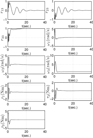
Figure 2: Time-response of attitude dynamics

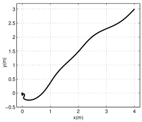
Figure 3: $(x,y)$ trajectory

The simulation is repeated with $R(0)=\left[\begin{array}[]{ccc}1&0&0\\ 0&-1&0\\ 0&0&-1\end{array}\right]$ while all other initial condition remaining the same. The time-response is shown in Figure 4 and the $(x,y)$ trajectory is shown in Figure 5.

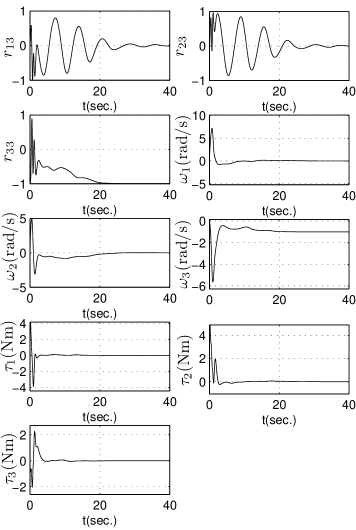
Figure 4: Time-response of attitude dynamics

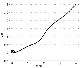
Figure 5: $(x,y)$ trajectory

A consequence of the control law is the regulation of $\Omega$ to $e_{3}$, which implies a) $\omega=e_{3},r_{3}=e_{3}$ as seen in Figure 2 or b) $\omega=-e_{3},r_{3}=-e_{3}$ as seen in Figure 4.

6 Conclusions

In this paper we have presented a smooth geometric controller to asymptotically stabilize the system to a smooth submanifold. This results in the robot reaching the origin of the plane while the robot spins with constant angular velocity about its local spin-axis, which by design is the body $Z_{b}$-axis coincident with the inertial $Z_{i}$-axis. This control strategy can be used in line-of-sight application for payload pointing, such as a camera mounted inside the sphere.

References

- [1] F. Bullo and A. D. Lewis, Geometric Control of Mechanical Systems. Springer, 2005.
- [2] J. Osborne, G. Hicks, and R. Fuentes, “Global analysis of the double-gimbal mechanism: Dynamics and control on the torus,” IEEE Control Systems Magazine, vol. 28, no. 4, pp. 44–64, 2008.
- [3] T. Lee, M. Leok, and N. H. McClamroch, “Geometric tracking control of a quadrotor UAV for extreme maneuverability,” in Proceedings of the 18th IFAC World Congress, (Milano, Italy), August 2011.
- [4] A. M. Bloch, Nonholonomic Mechanics and Control. Department of Mathematics, University of Michigan, Ann Arbor: Springer, Science, 1995.
- [5] A. Koshiyama and K. Yamafuji, “Design and control of an all-direction steering type mobile robot,” International Journal of Robotics Research, vol. 12, no. 5, pp. 411–419, 1993.
- [6] A. Bicchi, A. Balluchi, D. Prattichizzo, and A. Gorelli, “Introducing the “sphericle” : an experimental testbed for research and teaching in nonholonomy,” in IEEE International Conference on Robotics and Automation, (Albuquerque, New Mexico), April 1997.
- [7] S. Bhattacharya and S. K. Agrawal, “Spherical rolling robot: A design and motion planning studies,” IEEE Transactions on Robotics and Automation, vol. 16, no. 6, pp. 835–839, 2000.
- [8] T. Das and R. Mukherjee, “Reconfiguration of a rolling sphere: a problem in evolute-involute geometry,” ASME Journal of Applied Mechanics, vol. 73, pp. 590–597, 2006.
- [9] J. Shen, D. A. Schneider, and A. M. Bloch, “Controllability and motion planning of a multibody Chaplygin′s sphere and Chaplygin′s top,” International Journal of Robust and Nonlinear Control, vol. 18, pp. 905–945, 2008.
- [10] H. Karimpour, M. Keshmiri, and M. Mahzoon, “Stabilization of an autonomous rolling sphere navigating in a labyrinth arena: A geometric mechanics perspective,” Systems and Control Letters, vol. 61, pp. 494–505, 2012.
- [11] S. Gajbhiye and R. N. Banavar, “The Euler-Poincaré equation for a spherical robot actuated by a pendulum,” in Proceedings of the 4th IFAC Workshop on Lagrangian and Hamiltonian Methods for Nonlinear Control, (Bertinoro, Italy), pp. 72–77, August 2012.
- [12] R. W. Brockett, Asymptotic stability and feedback stabilization in Differential Geometric Control theory. MA: Boston, MA:Birkhauser, 1983.