Thermal interface fluctuations of liquids and viscoelastic materials

Abstract

Spectra of thermal fluctuations of a wide range of interfaces, from liquid/air, viscoelastic material/air, liquid/liquid, to liquid/viscoelastic material interfaces, were measured over 100 Hz to 10 MHz frequency range. The obtained spectra were compared with the fluctuation theory of interfaces, and found to be mostly in quite good agreement, when the theory was generalized to apply to thermal fluctuations of liquid/viscoelastic material interfaces. The spectra were measured using a system that combines light reflection, statistical noise reduction through averaged correlations, and confocal microscopy. It requires only a small area of the interface ($\sim 1\,\mu$m²) , relatively short times for measurements ($\lesssim$few min), and can also be applied to highly viscous materials.

I Introduction

Interfaces between various kinds of materials, such as gas, liquid, viscoelastic material, contain the physics of matter in the bulk, as well as the physics of the matter specific to the interfaces, making their study of fundamental interestintPhysics . The behavior of matter at interfaces is of interest, and has practical importance, also in a broad range of areas including properties of emulsions, lubrication, oil recovery and decontamination, as well as biological applicationsintGeneral . One effective approach in investigating the dynamics of interfaces is to study their thermal fluctuations non-invasively. While large thermal fluctuations in the critical regime have been seenLauter ; Giglio , generically the motions are at atomic scales, and measuring their properties with precision remains to be a challenging subject. Both for fundamental physics, and for practical applications, we believe it is important to investigate spontaneous fluctuations at interfaces in detail, and to understand the validity of fundamental theories that have been proposed to describe their behavior.

In this work, we directly measure the spectra of thermal fluctuations of various types of interfaces at room temperature, including liquid/liquid, and liquid/viscoelastic matter interfaces. Previously, thermal fluctuations of liquid/air and liquid/liquid interfaces, often called “ripplons”ripplon , have been observed in light scattering experiments, using propagating waves on the interfaces effectively as traveling gratingsripplonExp ; Domingo ; Sauer ; Sawada94 . Thermal fluctuations of liquid/viscoelastic material interfaces seem not to have been observed previously. Using light scattering to observe thermal fluctuations is difficult for interfaces involving liquids with large viscosity, since the waves dissipateSakaiVisc . The theory of thermal fluctuations of interfaces was worked out from first principles some time agoLevich ; Bouchiat ; HM ; Meunier ; HPP , yet it had not been possible to experimentally examine their behavior in detail. In this work, the fluctuations are observed using light reflection, with the interface effectively acting as an optical leverlever ; MitsuiOnion ; Tay ; MA1 , so that the method does not rely on the existence of waves that act as gratings. This allows us to measure properties of thermal fluctuations of previously inaccessible interfaces with precision, over a wide frequency range, including those involving highly viscous materials. The obtained fluctuation spectra were analyzed in view of the theory, which was generalized to apply also to liquid/viscoelastic material interfaces. The results mostly show good agreement with the theory, but aspects that need to be further investigated remain.

II Experimental concept and scheme

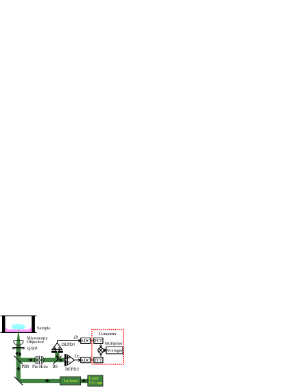
Figure 1: The setup of the measurement system: Light from the laser source (wavelength 532 nm) is stabilized using an isolator, and is focused on the sample interface between two media (blue, pink). Using a quarter-wave plate (QWP), the light from the sample is reflected at the polarized beam splitter (PBS). A pin hole is used for confocal microscopy. The reflected light is partitioned in two by a beam splitter (BS) and the light beams are detected by dual-element photodiodes (DEPD1,2). The measured photocurrents are digitized by analog-to-digital converters (ADC), and processed on a computer.

To investigate the behavior of interfaces precisely, the basic experimental concept we adopt is to measure the fluctuations in the average inclination of the interface in the light beam, which acts as a partial mirror. This basic principle is realized in the experimental setup shown in Fig. 1: A light beam is focused on the interface between two media, and is partially reflected. At any instant, the average direction of the reflected light deviates slightly from the incoming beam direction, due to interface fluctuations. These inclination fluctuations are measured through the photocurrent differential in a dual-element photodiode (DEPD), and their power spectrum is computed. Confocal microscopy is used to select only the fluctuations at the interface under investigation. The measurement method employed can be described as dynamic light reflection, and compared to dynamic light scattering, the signal is stronger for a given incoming light, so that a far weaker light source can be used.

For precision measurements, it is imperative to reduce the shot-noise, which appears as $2eI$ in the photocurrent ($e$ is the electron charge, and $I$ is the photocurrent). The shot-noise originates in the photon nature of light, and can potentially overwhelm the signal. One option is to increase the light power, which will, in general, affect the sample significantly, and in the problem at hand, it is not possible to increase the light powers to levels where the spectra can be recovered to the desired accuracy without doing so. In this work, we reduced the shot-noise statistically, as follows: The light reflected from the interface is split into two beams, whose (time-dependent) powers are measured independently by photodetectors as ${D}_{1,2}$. These measurements, ${D}_{j}=S+N_{j}$, contain both the signal, $S$, and the noise, $N_{j}$, such as shot-noise, that occurs independently in the photocurrents. By repetitively taking the correlation of the Fourier transform of these measurements, and averaging over them, the desired spectrum is obtained in the limit of infinite number of averagings, $\langle\overline{\tilde{D}_{1}}\tilde{D}_{2}\rangle\longrightarrow\langle|\tilde{S}|^{2}\rangle$. Here, $\langle\cdots\rangle$ denotes ensemble averaged results, and tilde denotes the Fourier transform. Any noise that is decorrelated in the two measurements, including the shot-noise and amplifier noise, is reduced statistically in the correlation $\langle\overline{\tilde{N}_{1}}\tilde{N}_{2}\rangle$, by a factor $1/\sqrt{{\cal T}\Delta f}$, $\Delta f$ being the frequency resolution, ${\cal T}$ the total measurement time. This reduction is statistical, and is consistent with the statistical fluctuations of the photons, since the total number of observed photons has increased by a factor of ${{\cal T}\Delta f}$, the number of averagings. Taking the correlation of independent measurements here is crucial, since without it, the shot-noise is not reduced. This principle for reducing the shot-noise has been used to achieve factors of $10^{-3}$ to $10^{-5}$ reduction, in the measurements of surface thermal fluctuations of fluidsMA1 ; MA2 , spontaneous noise in atomic vaporMA3 ; MA4 , and reflectance fluctuationsMA5 .

Technical details of the setup (Fig. 1) are as follows: Light from a laser source (wavelength 532 nm), stabilized by an isolator, is focused on the interface between two materials close to the diffraction limit, using a microscope objective with a correction mechanism for the aberration caused by the material below the interface, and a numerical aperture ($N\!A$) of 0.6. The materials were contained in a cylinder with a inner diameter of 12.2 mm. The total light powers applied on the interfaces varied from $0.4$ to $1.0$ mW. A quarter-wave plate is included in the light path to reflect the light coming from the sample interface at the polarized beam splitter. Using confocal microscopy, a pin hole is placed in the reflected light beam path to select out the light reflected from the interface. The light reflected at the sample interface is then split in two using a beam splitter, and the light beam powers are measured using dual-element photodiodes (DEPD’s). The two reflected light beams are so directed that the light powers in the two photodiodes in each of DEPD1,2 are identical, apart from noise. Fluctuations cause the interface to act as an optical leverlever , causing differences in the photocurrents from DEPD. These differential photocurrents are fed through an analog-to-digital converter into a computer, which computes their Fourier transforms (FFT), correlations, and averages. Measurement times for the spectra obtained below varied from 15 seconds to 7 minutes, depending on the reflectance of the interface, the magnitude of the fluctuations, and the desired precision. The average inclination, $\theta$, of the surface within the beam spot is related to the photocurrents in the two elements in DEPD’s as $(I_{j1}-I_{j2})/(I_{j1}+I_{j2})=2\theta/N\!A$, where $I_{j1},I_{j2}$ are the photocurrents from the two elements in DEPD$j\ (j=1,2)$. Since the light beam diameter is slightly smaller than that of the microscope objective, $N\!A$ can effectively be smaller than its catalog value. The power spectrum is computed in the standard fashionSpectrumRef , as $S(\omega)=\langle|\tilde{\theta}|^{2}\rangle/{\cal T}={\rm const.}\times\langle\overline{\tilde{D}_{1}}\tilde{D}_{2}\rangle/{\cal T}$, where $\omega$ is the angular frequency.

III Interfaces of liquids

Theoretically, the fluctuation spectrum of the inclinations of the surface is

$$S(f)=\int_{0}^{\infty}dq\,q^{3}e^{-w^{2}q^{2}/4}P(q,\omega)\quad,$$ (1)

where $P(q,\omega)$ is the spectral function for the interface fluctuations, and $w$ is the beam spot radius, and $q$ denotes the wave number MA1 ; AM1 . Since the observed inclination of the surface is averaged within the beam spot, fluctuations with shorter wavelengths are effectively cutoff by a Gaussian factor. The spectral function for the thermal interface fluctuations between two fluids, described by densities $\rho_{1,2}$, shear viscosities $\eta_{1,2}$, and interface tension, $\sigma$ has been derived in HM ; Meunier ;

$$P(q,\omega)=-{k_{\scriptscriptstyle\rm B}T\over\pi\omega}{q\over\rho_{1}+\rho_{2}}{\rm\,Im\,}F^{-1},\quad F\equiv{1\over\tau_{0}^{2}}\left[y+s^{2}+2s{(\eta_{1}+\eta_{2}m_{2})(\eta_{2}+\eta_{1}m_{1})\over(\eta_{1}+\eta_{2})\left[\eta_{1}(m_{1}+1)+\eta_{2}(m_{2}+1)\right]}\right]\quad,$$ (2)

$$\tau_{0}={\rho_{1}+\rho_{2}\over 2(\eta_{1}+\eta_{2})q^{2}},\quad y={\sigma(\rho_{1}+\rho_{2})\over 4(\eta_{1}+\eta_{2})^{2}q},\quad s=i\omega\tau_{0},\quad m_{j}=\sqrt{1+i{\rho_{j}\omega\over\eta_{j}q^{2}}},\quad(j=1,2)\quad,$$ (3)

where we have also made use of the expressions in Loudon ; Loudon2 . Gravity affects interface fluctuations in the region where the wavelength is larger than $2\pi\sqrt{\sigma/(|\rho_{1}-\rho_{2}|g)}$, where $g$ is the gravitational acceleration. These fluctuations have wavelengths of few centimeters or larger, which are suppressed by the experimental geometry, so will not be considered below. The spectral function generalizes that of the surface (liquid/air interface)Bouchiat , to which it reduces to in the limit $\rho_{1},\eta_{1}\rightarrow 0$, assuming medium 1 is air. The spectral function for the liquid surface (liquid/air interface) was generalized to surface fluctuations of polymer solutions, by incorporating the contributions from the polymer network effectively into the fluid viscosity asHPP

$$\eta=\eta_{0}+{G\tau\over(1+i\omega\tau)}$$ (4)

Here, $\eta_{0}$ is the viscosity of the solvent, $G$ is the shear modulus, and $\tau$ is the stress relaxation time. Polymer gel surface fluctuation spectral function is obtained in the limit, $\tau\rightarrow\infty$.

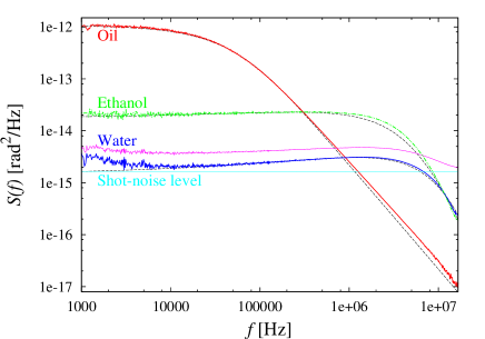
Figure 2: Measured surface fluctuation spectra for water (blue), ethanol (green), and oil (red). The corresponding spectra derived from theory are also shown (black dashes), which agree with the results well. For the water surface, the spectrum measured without using averaged correlations is also shown (magenta), along with the corresponding shot-noise level (cyan). Without using correlations, the spectrum contains the shot-noise, and differs visibly from the spectrum without the shot-noise.

In Fig. 2, the measured surface inclination fluctuations for water, ethanol and oil (Olympus immersion oil AX9602, here and below) are shown, along with their theoretical spectra, computed from Eq. (1),(2). Density, viscosity, surface tension, temperature of the fluids were $(\rho_{2}\,{\rm[kg/m^{3}]},\eta_{2}\,{\rm[Pa\cdot s]},\sigma\,{\rm[N/m]},t\,[\rm\degree C])=(9.98\times 10^{2},7.26\times 10^{-2},9.58\times 10^{-2},22),(7.89\times 10^{2},2.25\times 10^{-2},1.15\times 10^{-3},22),(9.20\times 10^{2},3.00\times 10^{-2},0.124,24)$, respectivelyProp , and $w=0.6\,\mu$m. The theory and the experiment are seen to agree well. These spectra are essentially the same as those measured in MA1 , except that the light was shone from inside the liquid, in contrast to the previous work, in which the light was shone from outside the liquid. For the water surface, the fluctuation spectrum obtained by averaging $\langle|\tilde{D}_{j}|^{2}\rangle\ (j=1,2)$, without using correlations, is also shown, along with the corresponding shot-noise level. Clearly, the spectrum differs significantly from that with the shot-noise removed. The noise level in an interface inclination fluctuation spectrum originating in the shot-noise, which we call the “shot-noise level” for brevity, is $N\!A^{2}e/(4In^{2})$, where $n$ is the index of refraction of the lower medium in Fig. 1, and $I$ is the photocurrent per photodiode. The overall magnitudes of the spectra were normalized by their corresponding theoretical spectra. For all the spectra shown in Fig. 2 and below, this shot-noise level computed using the photocurrent agreed with the observed shot-noise levels within experimental uncertainties.

Thermal surface fluctuations of liquids, often called “ripplons”ripplon , have previously been observed using surface light scattering, using the surface waves as gratingsripplonExp . In these measurements, the spectral function for particular wave numbers are obtained. In contrast, in our measurements, the spectrum integrated over the wave number up to the scale of inverse of the beam spot radius is obtained. With previous surface scattering methods, surface fluctuations of highly viscous liquids were difficult to measureSakaiVisc , whereas there is no additional effort involved for such liquids with our method.

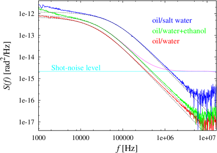
Figure 3: Measured inclination fluctuation spectra for interfaces of oil with water (red), salt water (concentration 16 %, blue), and water-ethanol mixture (20 % ethanol, green). The corresponding spectra derived from theory are also shown (black dashes), which are quite consistent with the experimental results. The spectrum measured without using averaged correlations is shown for the oil-water interface (magenta), with the corresponding shot-noise level (cyan). Higher frequency fluctuations are dominated by the shot-noise, unless it is removed.

In Fig. 3, the thermal inclination fluctuation spectra for interfaces of oil with water, salt water (concentration 16 %), and water-ethanol mixture (20 % ethanol), are shown. Corresponding theoretical spectra obtained from Eq. (2) are also shown for each spectrum, which agree with the experimental results well. The density and viscosity of oil are common to these measurements, $(\rho_{1}\,\rm[kg/m^{3}],\eta_{1}\,[Pa\cdot s])=(920,0.124)$, and for the water solutions, interface tension, beam radius, and the temperature were $(\rho_{2}\,{\rm[kg/m^{3}]},\eta_{2}\,{\rm[Pa\cdot s]},\sigma\,{\rm[N/m]},w\,{\rm[\mu m]},t\,[\rm\degree C])=(998,9.58\times 10^{-4},0.026,1.2,22),(1121,1.37\times 10^{-3},0.030,0.525,24),(973,1.72\times 10^{-3},0.026,1.0,22)$, respectively. Here, we adopted the known properties for the bulk properties of water solutionsProp ; SaltWater ; Ethanol . The interface tension values obtained here seem consistent with the theory, and previous measurementsFowkes ; FisherFood ; KimBurgess . The shape of the fluctuation spectra for these interfaces are similar to each other, and also to that of the oil/air interface in Fig. 2. Theoretically, the strong viscosity of oil dominates the spectra, and they should not have visible dependence on the concentration, unless the interface tension is changed, which is consistent with our measurements. The concentrations of salt and ethanol were systematically varied up to the levels seen in Fig. 3, but differences in interface fluctuation spectra due to the concentration were not observed, which is consistent with previous interface tension measurementsGaonkar . The differences observed in Fig. 3 can be attributed to the differences in the values of $w$. Theoretically, from the spectral function Eq. (2), the properties of the spectra are governed in large part by the most viscous fluid, when the viscosities of the fluids are widely different, as is the case here. The shot-noise level for the oil/water-ethanol mixture interface is additionally indicated in Fig. 3, and it can be seen that fluctuations at higher frequencies are buried below the shot-noise, if this is not reduced. Liquid/liquid interface fluctuations involving such highly viscous fluids have not been previously measured, to our knowledge, due to the absence of persistent waves, and the small reflectance of the interface. The frequency regions around the peak in the spectral functions have been observed previously for less viscous liquids Domingo ; Sauer ; Sawada94 , but fluctuations over a wide frequency range, especially including the high frequencies have not been previously observed.

IV Interfaces of liquids and viscoelastic materials

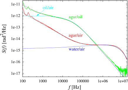
Figure 4: Observed inclination fluctuation spectra of agar/air (red) and agar/oil (green) interfaces. The corresponding theoretical spectra (black dashes) agree quite well with the observed spectra. Theoretical spectrum for water/air interface fluctuations (blue) agree well with the agar/air interface fluctuations at higher frequencies ($f\gtrsim 10^{6}$ Hz). The theoretical oil/air spectrum (cyan) matches the observed agar/oil spectrum well for higher frequencies, but not as well at lower frequencies ($f\lesssim 10^{4}$ Hz).

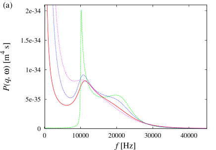
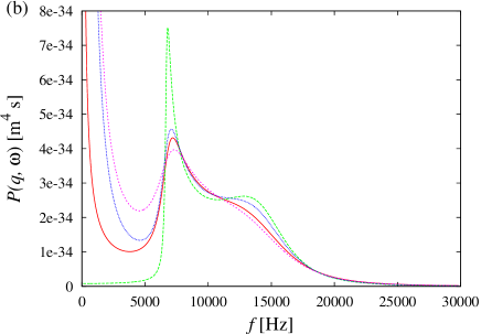
Figure 5: Comparison of the behaviors of the surface thermal fluctuation spectral function, $P(q,\omega)$, for polymer gel with loss modulus (red, solid), without (green, long dashes), polymer sol with loss modulus (blue, dots), and without (magenta, short dashes). The parameters used were, for (a), $\rho=10^{3}\,\rm kg/m^{3},\ \sigma=0.073\,N/m,\ \eta=10^{-3}\,Pa\cdot s,$, $G=(2.5\times 10^{3}+i1.0\times 10^{3})\rm\,Pa,\ \tau=5\times 10^{-5}\,s$, and for (b), $\rho=7.3\times 10^{2}\,\rm kg/m^{3},\ \sigma=0.024\,N/m,\ \eta=8\times 10^{-4}\,Pa\cdot s$, $G=(8.0\times 10^{2}+i1.5\times 10^{2})\,\rm Pa,\ \tau=1.5\times 10^{-4}\,s$. ${\rm\,Im\,}G=0$ when loss modulus is not considered, and $\tau$ is infinite for gels. $q=4\times 10^{4}{\rm\,m^{-1}},$ and $t=27\,$°C, both for (a), and (b).

In Fig. 4, the inclination fluctuation spectra for agar/air, and agar/oil interfaces are shown, along with the corresponding theoretical spectra (agarose gel is Agar, Difco 214220 2.6 wt % in water). The theoretical spectrum for the agar/air interface was obtained using the formalism of HPP in Eq. (2), with $G=(2.5\times 10^{3}+i1.0\times 10^{3})$ Pa, $w=0.65\,\mu$m, $t=24\,\degree$C, the properties of water as the solvent, which reproduces the observed spectra quite well. $G$, which is not real, contains both the shear modulus, and the loss modulus. At low frequencies, the leading behavior for the spectrum is ${\rm\,Re\,}\eta/(\sigma^{2}w)$AM1 , so that it falls off as $f^{-1}$ when ${\rm\,Im\,}G\not=0$, and behaves as a constant when ${\rm\,Im\,}G=0$ (or as $f^{-2}\tau^{-1}$ for sols). Therefore, the effect of the non-zero loss modulus is clearly visible in the spectrum above, for $f\lesssim 200\,$kHz. Viscoelastic material/air interface fluctuations have been observed previously with light scattering techniquesCao91 ; Kikuchi91 ; Dorshow93 ; Cao95 ; Huang96 ; Monroy , where a non-zero loss modulus was not considered, though viscoelastic materials have non-zero loss moduli, in generalFerry . The effect of the loss modulus is significant in the region, ${\rm\,Im\,}G/(\eta_{0}\omega)\gtrsim 1$. On the other hand, at relatively high frequencies, and relatively high wave numbers associated to it through the dispersion relation Eq. (2), the effect is small, which can explain why it had not been noticed previously. This is illustrated in Fig. 5, where the theoretical spectral behaviors of polymer gels and sols, with or without the loss modulus are compared, for parameters pertinent to our experiment in (a), and for parameters in the typical range for past measurements, such as those of polyisobutylene decane solutionsCao91 ; Dorshow93 ; Huang96 , in (b). It can be seen that polymer gel with the loss modulus, and polymer sol, both introduce dissipation to the dispersion relation peak in the gel spectral function, leading to similar behaviors around it. However, the behaviors at lower frequencies are qualitatively different, constant for gel without the loss modulus, $f^{-1}$ with it, and $f^{-2}$ for sols. In Fig. 4, it can also be seen that the high frequency fluctuations ($f\gtrsim 3\times 10^{5}\,$Hz) are well described by properties of the solvent, water. The values of shear and loss modulus seem to be consistent with those measured beforeMonroy ; Kikuchi94 , and also with those measured by other methodsTokita ; Fujii .

For the theory of thermal fluctuations of the agar/oil interface, we generalize the interface fluctuation formula Eq. (2) HM ; Meunier , by incorporating the polymer network contributions, as was done for the surfaceHPP . While this generalization has not been presented before, it is a natural one that can be derived much in the same mannerMeunier ; HM ; HPP . Applying this theory, with the value of $G$ used for the agar/air interface, $w=0.9\,\mu\rm m$, and $t=24\degree C$, the computed spectrum matches excellently with the observed spectrum (Fig. 4). For comparison, the theoretical surface fluctuation spectrum of oil with the same surface tension is shown, and it can be seen that a qualitative difference exists for low frequencies ($f\lesssim 10^{4}\,$Hz), while the higher frequency fluctuations are dominated by the properties of oil. Interfaces fluctuations between liquids and viscoelastic materials have not been observed previously.

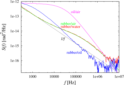
Figure 6: Observed inclination fluctuation spectra for the interfaces of silicone rubber with air (green), water (red), and oil (blue). For reference, the spectrum for the oil/air interface is also shown (magenta), along with its corresponding $1/f$ spectrum (black, dashes).

In Fig. 6, thermal inclination fluctuation spectra of silicone rubber (Tigers Polymer, SR 0.2 t, Japan) interface with air, water, and oil are shown ($w=0.6,\mu$m, $t=24\,$°C), along with that of the oil/air interface. Thermal fluctuations at interfaces of elastic materials and liquids seem not to have been observed previously. Since rubber is an elastic material with no solvent, its interface fluctuations can be obtained by taking the limit of viscosity going to zero in Eq. (2), which we shall use here. The spectral function computed this way differs from that obtained by other methodsSaulson90 ; Levin ; Braginsky99 by a dimensionless prefactor of order 1. Interestingly, rubber/air and rubber/oil interface spectra differ significantly, and unlike the agar/oil interface spectrum in Fig. 4, rubber/oil spectrum seems unrelated to the oil surface fluctuation spectrum, which is also shown for contrast. For rubber, if we assume that $G$ is frequency independent, the integrated spectrum behaves as $1/f$, in this frequency range. In Fig. 6, we compared the measured thermal fluctuation spectrum to the theoretical one computed with $G=(3.5\times 10^{6}+i3.5\times 10^{5})\,$Pa, which captures the overall spectrum but not the deviations from the $1/f$ behavior. This is not surprising since the loss modulus of rubber is frequency dependent, and the value of $G$ seems consistent with the known properties Ferry ; Sperling . The thermal fluctuation spectrum of rubber/water interface is essentially indistinguishable from that of rubber/air interface in Fig. 6, and this is quite consistent with the spectrum formula applied to these interfaces. It is seen in Fig. 6 that the thermal fluctuation spectrum for the rubber/oil interface differs qualitatively from that of rubber/air, or water interfaces. To understand this, the frequency dependence of the shear and loss moduli needs to be considered.

In this work, we measured the thermal fluctuation spectra of various types of interfaces; liquid/air, viscoelastic material/air, liquid/liquid, and liquid/viscoelastic material. The corresponding inclination fluctuation spectra were computed by combining the fluctuation theory of interfacesMeunier ; HM with that of surfaces of viscoelastic materialsHPP , and generalizing them. The theoretically computed spectra were, for the most part, found to be in excellent agreement with the experimentally observed spectra. We find it intriguing that the elegant simple formalism of Levich ; Bouchiat ; HM ; Meunier ; HPP can describe the whole spectrum of a wide range of interface fluctuations quite well, when the loss modulus is also considered. For the interface fluctuation spectra involving rubber, it was found that the frequency dependence of the elastic constants of the material was perhaps necessary to explain the spectra fully. We believe that the measurement system enables direct measurements of interface phenomena that were previously inaccessible, leading to a better understanding of the underlying fundamental theories. This measurement system we developed for the thermal interface fluctuations combines light reflection measurement, noise reduction through averaged correlations, and confocal microscopy. It is applicable to a wide variety of interfaces, as seen in this work. Some features of this system is that it can be applied to obtain fluctuation spectra of interfaces involving highly dissipative materials, requires only a small area (beam spot radius $\lesssim 1\,\mu$m) , and relatively low light powers ($\simeq 1\,$mW). It takes a short time to take a measurement (typically under a few minutes), which is determined by the desired precision. The system might also be suited for non-invasive measurements in biological and medical applications. Light reflection measurements of fluctuations, while seemingly similar to the more standard light scattering measurements, can also yield information regarding small wave number and low frequency behavior, complementing them.

References

- (1) C.A. Croxton (ed), “Fluid Interfacial Phenomena”, John Wiley & Sons, New York (1986).
- (2) A.G. Volkov (ed), “Liquid Interfaces In Chemical, Biological And Pharmaceutical Applications”, Marcel Dekker, New York (2001).
- (3) H.J. Lauter et al, Phys. Rev. Lett 68, 2484 (1992)
- (4) A. Vailati, M. Giglio, Nature 390, 262 (1997)
- (5) M. von Schmoluchowski, Ann Physik 25, 225 (1908); L. Mandelstam, Ann. Physik 41, 609 (1913).
- (6) D. Langevin (ed), “Light scattering by liquid surfaces and complementary techniques”, Marcel Dekker, New York (1992).
- (7) D. Jon, H.L. Rosano, H.Z. Cummins, J. Coll. Int. Sci. 114, 330 (1986).
- (8) B.B. Sauer, Y-L. Chen, G. Zografi, H. Yu, Langmuir 4, 111 (1988).
- (9) S. Takahashi, A. Harata, T. Kitamori, T. Sawada, Anal. Sci. 10, 305 (1994).
- (10) Y. Minami, K. Sakai, Rev. Sci. Inst. 80, 014902 (2009).
- (11) V.G. Levich, “Physicochemical Hydrodynamics”, Prentice-Hall, Englewood Cliffs (1962).
- (12) M.-A. Bouchiat, J. Meunier, J. de Phys. 32, 561 (1971).
- (13) J.C. Herpin, J. Meunier, J. Phys. 35, 847 (1974).
- (14) J. Meunier, “Surface critical opalescence”, in Langevin (Ed), “Light scattering by liquid surfaces and complementary techniques”, Marcel Dekker, New York (1992).
- (15) J.L. Harden, H. Pleiner, P.A. Pincus, J. Chem. Phys., 94, 5208—5221 (1991) .
- (16) R.V. Jones, J. Sci. Inst. 38, 37 (1961).
- (17) T. Mitsui, Jpn. J. Appl. Phys. , 44, 3279 (2005).
- (18) A.Tay et al., Rev. Sci. Instrum. 79, 103107 (2008).
- (19) T. Mitsui, K. Aoki, Phys Rev E80, 020602(R) (2009).
- (20) T. Mitsui and K. Aoki, Phys. Rev. E 87, 042403 (2013).
- (21) T. Mitsui, K. Aoki, Eur. Phys. J. D67, 213 (2013).
- (22) K. Aoki, T. Mitsui, Phys. Rev. A 94, 012703 (2016).
- (23) T. Mitsui, K. Aoki, Phys. Rev. A 95, 043821 (2017).
- (24) C.W. Gardiner, “ Handbook of Stochastic Methods”, Springer-Verlag, Berlin, (1985).
- (25) K. Aoki, T. Mitsui, Phys. Rev. E 86, 011602 (2012).
- (26) R. Loudon, J. Phys. 45, C5: 93 (1984).
- (27) R. Loudon, in Agranovich, Loudon (ed), “Surface Excitations” (1984).
- (28) W.M. Haynes (ed), “CRC Handbook of Chemistry and Physics”, CRC Press, Boca Raton (2011).
- (29) M.H. Sharqawy , J.H. Lienhard V, S.M. Zubair, Desalin. Water Treat. 16, 354 (2010).
- (30) I.S. Khattab, F. Bandarkar, M.A.A. Fakhree, A. Jouyban, Korean J. Chem. Eng. 29, 812 (2012) .
- (31) F.M. Fowkes, J. Phys. Chem. 66, 382 (1962); F.M. Fowkes, J. Phys. Chem. 67, 2538 (1963).
- (32) I.R. Fisher, E.E. Mitchell, N.S. Parker, J. Food Sci. 50, 1201 (1985).
- (33) H. Kim, D.J. Burgess, J. Coll. Int. Sci. 241, 509 (2001).
- (34) A.G. Gaonkar, J. Coll. Int. Sci. 149, 256 (1992).
- (35) B.H. Cao, M.W. Kim, H. Schaffer, J. Chem. Phys. 95, 9317 (1991).
- (36) H.Kikuchi, K. Sakai, K. Takagi, Jpn. J. Appl. Phys. 30, L1668 (1991).
- (37) R.B. Dorshow, L.A. Turkevich, Phys. Rev. Lett. 70, 2439 (1993).
- (38) B.H. Cao, M.W. Kim, H.Z. Cummins, J. Chem. Phys. 102, 9375 (1995).
- (39) Q.R. Huang, C.H. Wang, J. Chem. Phys. 105, 6546 (1996); Q.R. Huang, C.H. Wang, N.J. Deng, J. Chem. Phys. 108, 3827 (1998).
- (40) F. Monroy, F, D. Langevin, Phys. Rev. Lett. 81, 3167 (1998).
- (41) J.D. Ferry, “Viscoelastic Properties of Polymers”, John Wiley & Sons, New York (1980).
- (42) H. Kikuchi, K. Sakai, K. Takagi, Phys. Rev. B49, 3061 (1994).
- (43) M. Tokita, K. Hikichi, Phys. Rev. A35, 4329 (1987).
- (44) T. Fujii, T. Yano, H. Kumagai, Biosci. Biotechnol. Biochem. 64, 1618 (2000).
- (45) P.R. Saulson, Phys. Rev. D42, 2437 (1990)
- (46) Y. Levin, Phys. Rev. D57, 659 (1998)
- (47) V.B. Braginsky, M.L. Gorodetsky, S.P. Vyatchanin, Phys. Lett. A264, 1 (1999)
- (48) L.H. Sperling, “Introduction to polymer science”, John Wiley & Sons, New York (2006).