Stationary ordered non-equilibrium states of long-range interacting systems

Abstract

Long-range interacting Hamiltonian systems are believed to relax generically towards non-equilibrium states called “quasi-stationary" because they evolve towards thermodynamic equilibrium very slowly, on a time-scale diverging with particle number. We show here that, by applying a suitable perturbation operator for a finite time interval, we obtain, in a family of long-range systems, non-equilibrium states which appear to be strictly stationary. They exist even in the case of a harmonic potential, and are characterised by an ordered microscopic phase space structure. We give some simple heuristic arguments which predict reasonably well some properties of these states.

Long-range interacting systems are ubiquitous in nature and concern diverse physical situations (for an overview see e.g. Campa et al. (2014)) from very large length scales as self-gravitating bodies in astrophysics Padmanabhan (1990); Binney and Tremaine (2008), to very small length scales such as cold atom systems Chalony et al. (2013); Barré et al. (2014), plasmasNicholson (1983), free-electron lasersBarré et al. (2004) as well as chemotaxis in biological systemsKeller and Segel (1971); Sire and Chavanis (2002). One of the apparently universal features of these systems is that the dynamics of their relaxation to microcanonical equilibrium is extremely slow: the time-scale for it is typically found to diverge as a positive power of particle number (see e.g. Farouki and Salpeter (1982); Yamaguchi et al. (2004); Joyce and Worrakitpoonpon (2010); Gabrielli et al. (2010); Teles et al. (2010); Marcos et al. (2017)). On mean-field time-scales, however, the systems are observed to attain macroscopically stationary out-of-equilibrium states, interpreted as stationary states of the Vlasov equation. These states, known as “quasi-stationary” states (QSS) because of their slow evolution towards equilibrium, are of fundamental physical importance, as they represent essentially macroscopic equilibria of a large class of Hamiltonian systems. Many basic questions about them remain, concerning notably both the mean-field dynamics leading to the QSS and their long-time relaxation dynamics. Several authors (see e.g. Gupta and Mukamel (2010); Nardini et al. (2012); Patelli et al. (2012); Chavanis et al. (2011)) and we ourselves Joyce et al. (2014, 2016) have investigated the interesting issue of whether QSS may or may not persist in the presence of perturbations to the Hamiltonian dynamics. Our study has revealed a rather unexpected and intriguing result which is the subject of this Letter: a particular class of perturbations, applied to such systems for a finite time, can drive them efficiently to states of the $N$ body system which, like QSS, are macroscopically stationary on mean field times scales but, unlike QSS, do not evolve at all (on the very longest time-scales we can access numerically). Microscopically these states are very different to typical QSS, as they are characterised by a highly regular “ordered” structure in phase space corresponding to periodic or quasi-periodic solutions of the $N$-body Hamiltonian dynamics.

Specifically we consider here one dimensional long-range interacting systems with interparticle potential $V(r)=gr^{\alpha}$ where $r$ is the distance between particles and $sgn(g)=sgn(\alpha)$ (i.e. attractive forces). The numerical results reported below are for the case $\alpha=1$, corresponding to the so-called “sheet model" , equivalent to infinite, infinitely thin, parallel sheets moving in three dimensions under Newtonian self-gravity (see e.g. Miller (1996); Yawn and Miller (1997); Joyce and Worrakitpoonpon (2010) and references therein). As detailed in the Supplemental Material, we have explored a large range of values for the exponent $\alpha$ in the range $[-1,2]$ and found our essential results to hold in this entire range, provided a suitable regularisation of the singularity at $r=0$ is employed for $\alpha<1$. The model with $\alpha=2$ is equivalent to a set of uncoupled identical harmonic oscillators, for which the dynamics is thus evidently non-ergodic, while in other cases studies suggest that it is expected to be ergodic Milanović et al. (2006, 1998), at least for a sufficient number of particles. Specifically, for the case $\alpha=1$, using an analysis of the stability of periodic orbits Reidl and Miller (1993) have concluded that ergodicity applies for $N>11$. Ergodicity breaking is quite ubiquitous for long range interacting systems Borgonovi et al. (2004); Bouchet et al. (2008); Mukamel et al. (2005); Teles et al. (2010); Benetti et al. (2012), but that we discuss here has a completely different origin to previous studies.

Using molecular dynamics simulations, we study these models with a simple modification: for a certain finite duration we modify the Hamiltonian dynamics by implementing a non-trivial collision rule when particles cross one another. Assuming momentum conservation, any such rule can be written

$$v_{i}^{*}= v_{j}+f(v_{ij})\,v_{ij}$$

$$v_{j}^{*}= v_{i}-f(v_{ij})\,v_{ij}$$

where $v_{i}$ ($v_{i}^{*}$) and $v_{j}$ ($v_{j}^{*}$) are the velocities of the particles before (after) the collision, and $f$ any function of the absolute value of the relative velocity $v_{ij}=v_{i}-v_{j}$ only, and the change in the kinetic energy is

$$\delta K=-mf(v_{ij})\left[1-f(v_{ij})\right]v_{ij}^{2}$$ (1)

The family of collision rules we use here are ones for which $\delta K<0$ when $|v_{ij}|<v_{0}$, and $\delta K>0$ when $|v_{ij}|>v_{0}$, where $v_{0}$ is a constant positive velocity, i.e., energy is injected when the particles cross at a relative velocity of less than $v_{0}$, and is dissipated if it is greater (and conserved when $v=v_{0}$). This is a generalisation of a collision rule introduced by Brito et al.Brito et al. (2013) in the context of a phenomenological model of an agitated granular gas, and for which

$$f(v)=q\left(1-\frac{v_{0}}{|v|}\right)$$ (2)

where $q$ is a dimensionless constant (controlling the degree of non-elasticity of the collisions). Our results below are for this specific rule, but we have explored a variety of quite different functional forms for $f(v)$ which have the required injection/dissipation structure. The results we obtain are all completely insensitive to these changes.

We will consider the limit here in which this inelastic collision rule constitutes a weak perturbation to the system. By this we mean that the time scale on which it causes non-trivial macroscopic evolution of the system is long compared to the characteristic time of the mean field dynamics. It is straightforward to show Joyce et al. (2016) that this corresponds to the requirement that $\gamma=qN$ be small, and thus to the quasi-elastic limit $q\rightarrow 0$ McNamara and Young (1993).

We report here results first for the case $\alpha=1$. Our initial conditions are “rectangular waterbag" — particles distributed with random uncorrelated positions in an interval $[-L_{0}/2,L_{0}/2]$ and random uncorrelated velocities in an interval $[-V_{0}/2,V_{0}/2]$ — characterised fully by the initial virial ratio $R=2K/U$ (where $K$ and $U$ are kinetic and potential energy respectively). Simulations are performed using the above collision rule from $t=0$ until a time $t^{*}\gg t_{dyn}/\gamma$ at fixed small $\gamma$ ($\sim 10^{-2}$) (where $t_{dyn}=2\sqrt{L_{0}/(gN)}$ is the mean-field time), and the purely Hamiltonian dynamics thereafter. Further details on the algorithm and numerics can be found in Joyce et al. (2016). For any $R$ we observe the same phases in the evolution. Fig. 1 shows the temporal evolution of two global observables, the virial ratio and the “entanglement” parameter, $\phi_{11}=\frac{\langle|xv|\rangle}{\langle|x|\rangle\langle|v|\rangle}$, which is equal to one if the system is in thermodynamic equilibrium Joyce and Worrakitpoonpon (2010). Firstly, on short time-scales ($t\ll t_{dyn}/\gamma$), the role of the perturbation is negligible and, as the evolution is indistinguishable from that of the Hamiltonian system, leads to relaxation towards a continuum of virialized states (with properties depending on $R$, see e.g. Joyce and Worrakitpoonpon (2010)). Secondly, for $t\sim t_{dyn}/\gamma$, the system evolves to a macroscopically stationary state and then progressively becomes “ordered” in the microscopic phase space until it reaches configuration which shows no further evolution. In Fig. 1 this non-trivial microscopic evolution corresponds to the very visible decay of the fluctuations in the macroscopic observables for $t<t^{*}$ and no further changes for $t>t^{*}$ when the perturbation is suppressed. In the final state $\phi_{11}\simeq 0.85$ which, we note, tells us that the system is definitely out of equilibrium.

When the perturbation is switched off, at $t=t^{*}$, not only is their no measurable change in the macroscopic evolution, but the same microscopic structure also persists. We have found this to be true no matter how long we have continued to evolve the system, and in particular for times very much longer than those observed for relaxation to equilibrium of typical QSS in this system, of order $(10-100)Nt_{dyn}$ Joyce and Worrakitpoonpon (2010). More precisely, we have observed no measurable evolution away from the ordered state up to $t=50000t_{dyn}$ for systems of size up to $N=128$. Although our results are purely numerical, they strongly suggest that the state which the system is driven to by perturbation is apparently a stable periodic or quasi-periodic solution of the exact $N$-body dynamics, and thus ergodicity is broken and the system will never relax to microcanonical equilibrium.

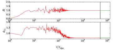
Figure 1: Time evolution of the virial ratio $R$ and the entanglement parameter $\phi_{11}$ for $N=128$ in the sheet model, and $t^{*}=5000\tau_{dyn}$ (black vertical line).

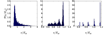
Figure 2: PDF of the total energy per particle at different times $t=10,100,1000t_{dyn}$ for a system of $N=128$.

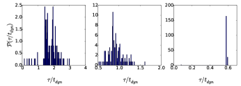
Figure 3: PDF of particle “periods" at different times for $N=128$.

To better understand the evolution towards this final state, we have monitored the probability distribution function (PDF) of the particle energies $e_{i}=\frac{1}{2}mv^{2}_{i}+\sum_{j\neq i}v(x_{i}-x_{j})$. Fig.2 shows, for a system with $N=128$, how this PDF evolves, from a wide distribution at early times ($t=10t_{dyn}$) to a very different form ($t=100t_{dyn})$ with several visible peaks of amplitude increasing with energy, which then become narrower until they are very well localised i.e. almost $\delta$-function peaks. The number of peaks is strongly dependent on, and grows with, the system size (see Fig.2).

The formation of these almost discrete peaks in particle energy corresponds in phase space to the existence of a ring structure. Further there is also a discrete structure within each ring (see Figs. 4-5) and a coherence between this structure in the different rings. Closer examination of the temporal evolution shows that, as one might suspect, the emergence of this ordered structures reflects a complete coherence of the particle motions. Figure 3 shows the PDF at different times of the particle “periods”, calculated for each particle as the time elapsed since it was last at the same position. At short times $t\sim\tau_{dyn}$, the PDF is broad, but it then evolves on time-scales at which the perturbation plays a role, initially changing shape and then converging to a very narrow peak as the final state is established. Again, when the perturbation is switched off, no measurable evolution of the PDF is observed. In the final state therefore all particles appear to move in a completely coherent periodic (or quasi-periodic) motion.

Given these observations, the trajectories can be written as a Fourier series with $x_{i}=\sum_{n\geq 1}\frac{V_{i,n}T}{2\pi}\cos(2\pi nt/T+\phi_{i,n})$ where $V_{i,n}$ is the corresponding coefficient of the Fourier expansion of the velocity. Figs. 4 and 5 show snapshots of the phase space configuration at $t=50000\tau_{dyn}$, for various system sizes for $N$ from $5$ to $16$ and for $N=20,25,30,35,40,45,50$. These plots are in the dimensionless variables $v/v_{0}$ and $x/x_{0}$, where $x_{0}=v_{0}T/(2\pi)$ and $T$ is the numerically estimated period. The time evolution of the system is illustrated for two particle sizes ($N=15$ and $N=128$) by the movies provided in the Supplemental Material. It is clear that, to a good approximation, the trajectories are circular, which implies that the term $n=1$ in the sum dominates, i.e., the trajectories are very close to those of harmonic oscillators. This phenomenon is only possible if the total force acting on each particle is almost independent of the number of particles and depends linearly on the distance of the particle to the center of mass of the system. In other words, the system reorganises due to the perturbation so that each particle behaves almost like an independent simple harmonic oscillator.

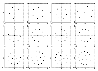
Figure 4: Snapshots of the final state after $50000\tau_{dyn}$ for $N=5,...,16$.

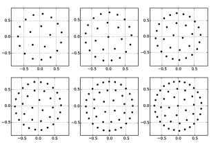
Figure 5: Snapshots of the final state after $50000\tau_{dyn}$ for $N=20,25,30,35,40,45,50$.

For systems up to $N=7$, the particles are located on a single circle. For $8\leq N\leq 11$, all but one of the particles are on a single circle while the remaining one is very close to the origin. For $N=12,13$ the structure in phase space is now composed of two circles of non-zero radii, the smaller with two particles and the larger with $N-2$ particles. For $N=14$, a third particle appears on the smaller circle. For $N$ varying from $N=20$ to $N=50$, the number of circles increases from $2$ ring structure for $N=128,256,512$ particles for which there are $6,8$ and $12$ circles respectively.

Given the regular spacing of the particles on each circle, supposing that there are $N_{c}$ circles, and that the $r$-th circle (where $r=1..N_{c}$) has $N_{r}$ particles (and thus $N=\sum_{r=1}^{N_{c}}N_{r}$), we can write the particle positions on a given circle as $x_{i}=\frac{VT}{2\pi}\cos(2\pi nt/T+2(i-1)\pi/N_{s}+\phi_{s})$ with $i=1..N_{s}$, and $V_{s,n}/v_{0}$ is the radius in phase space of the circle when plotted in the dimensionless variables as in Figs. 4 and 5. Note that we have made the approximation, which can be exact strictly only for the model $\alpha=2$ and not for the sheet model we are considering, that $V^{s}_{i,n}=0$ for $n>1$, i.e., that the orbits are those of perfectly decoupled and harmonic oscillators. The phase $\phi_{s}$ is the phase of the shell $s$ fixed by the position of the particle labeled $i=1$ at $t=0$, and without loss of generality, we can thus assume $\phi_{1}=0$.

Given the observed periodicity of the evolution in the stationary state, we must conclude that the total energy change due to collisions over one period is zero. As every particle collides with every other one twice in one period, this can be written

$$\delta E=\sum_{r=1}^{N_{c}}\sum_{s=1}^{N_{c}}\sum_{i_{r}=1}^{N_{r}}\sum_{j_{s}=1,j_{s}\neq i_{r}}^{N_{s}}\delta e_{i_{r}j_{s}}$$ (3)

where $\delta e_{i_{r}j_{s}}$ is the energy change due to a collision between a particle $i_{r}$ of the shell $r$ and a particle $j_{s}$ of the shell $s$. As we are working in the quasi-elastic limit, we have, using Eqs. (1-2), that $\delta e_{i_{r}j_{s}}=m\frac{\gamma}{N}[-v^{2}_{i_{r}j_{s}}+v_{0}|v_{i_{r}j_{s}}|]$ where $v_{i_{r}j_{s}}$ is the relative velocity for a pair of colliding particles. Since we can assume, in the quasi-elastic limit, that the particles are not perturbed from their circular orbits by the collisions which occur when particles are at the same spatial position, $v_{i_{r}j_{s}}$ is simply given by the (invariant) distance in phase space between the two particles. We therefore have that

$$|v_{i_{r}j_{s}}|=\sqrt{V_{r}^{2}+V^{2}_{s}-2V_{r}V_{s}\cos\left(\Phi\right)},$$ (4)

where $V_{r}$ and $V_{s}$ are the amplitudes of the velocities of particles $i_{r}$ and $j_{s}$, respectively, and the relative phase $\Phi=\frac{2i_{r}-2}{N_{r}}-\frac{2j_{s}-2}{N_{l}}+\phi_{r}-\phi_{s}$.

We first consider systems where all the particles are on a single circle, which we find (numerically) to be the case for $N\leq 8$. There is then just one free parameter, the dimensionless radius of the single circle in phase space $R_{1}=V_{1}/v_{0}$ in Fig.4. Using Eq.(4), Eq.(3) then gives

$$R_{1}=\frac{\sum_{i=1}^{N-1}\sin\left(i\frac{\pi}{N}\right)}{2\sum_{i=1}^{N-1}\sin^{2}\left(i\frac{\pi}{N}\right)}$$ (5)

In Table 1, we compare simulation results and theoretical predictions, Eq.(5). For these small system sizes ($N=5,6,7$) the uncertainty of the radii reported in Table 1 reflects the deviations from the assumed circular trajectories which decrease as $N$ grows.

For $N\geq 8$, our simulations starting from waterbag initial conditions always give rise to a final state with a single particle very close to the origin and the others very close to periodic motion on a single circle. Assuming the configurations to be given by one with one particle assumed to stay at rest at the origin and the other $N-1$ particles on the circle, there is again a single free parameter $R_{1}$ which is given by a simple expression derived from Eq. (4) taking $V_{2}=0$ and $V_{1}=v_{0}R_{1}$. The comparison of the numerical and theoretical results is shown again in Table 1. For $N=9,10,11$, we obtain the same stable configuration and have obtained $R_{1}$ using the same reasoning. For $N\geq 12,13$, our simulations, as we have noted give final configuration with at least two circles both with more than one particle. There is then more than one free parameter and the condition $\delta E=0$ can thus not determine the state uniquely. For two such circles we find, however, that we can obtain good predictions from this condition alone with some simple assumptions. In general there are in this case, given the observed number of particles on the two circles, three free parameters: the two dimensionless radii of the circles $R_{1}=V_{1}/v_{0}$ and $R_{2}=V_{2}/v_{0}$, and the phase $\phi_{2}$. In practice the condition is very weakly dependent on $\phi_{2}$, and so we set $\phi_{2}=0$. We then obtain the condition in the form of an implicit equation $f(R_{1},R_{2})=0$. We find that choosing the unique solution corresponding to the largest value of $R_{1}$, which corresponds to the largest value of the energy, we observe good agreement with simulation results. For the case of two circles plus a single particle at rest, an analogous calculation can be performed and gives again (see Table 1) satisfactory results for case $N=25$.

Numerically we find that in all cases the radius $R_{1}$ of the biggest circle always increases when a circle is added, and thus we expect that the limit $N\rightarrow\infty$ of Eq. (5), which gives $R_{1}=2/\pi$, should be a strict lower bound on its value. For larger systems (up to $N=512$) we observe also that the number of particles on the outer circle $N_{1}\simeq N/2$, and the value of $R_{1}$ in the configuration with the other $N-N_{1}$ particles at the origin, should thus give an upper bound on it. It is simple to show that this is $R_{1}=1/\pi+1/2$. Using the same reasoning, assuming all the particles on one circle, one obtains a lower bound on the parameter, $\phi_{11}=\pi/4=0.785..$, which is smaller than and comparable to the simulation results ($\phi_{11}=0.85$). We note that our observation of these apparently stable states for $N\geq 11$ appears to invalidate the analysis of Reidl and Miller (1993), who concluded that this system should be strictly ergodic in this case.

Table 1: Measured and predicted radii

$N$	Simulation	Predictions
$5$	$0.59\pm 0.02$	$0.615$
$6$	$0.60\pm 0.02$	$0.622$
$7$	$0.61\pm 0.02$	$0.6258$
$8$	$0.785\pm 0.03$	$0.6726$ (2 circles)
$9$	$0.602\pm 0.03$	$0.6697$ (2 circles)
$10$	$0.666$	$0.667$(2 circles)
$11$	$0.660$	$0.665$ (2 circles)
$12$	$0.23,0.66$	$0.25,0.702$ (2 circles)
$13$	$0.21,0.60$	$0.25,0.697$ (2 circles)
$20$	$0.32,0.717$	$0.31,0.74$ (2 circles)
$25$	$0,0.37,0.74$	$0,0.32,0.79,$ (3 circles)
$N$	Simulation	lower and upper bounds
$30$	$0.738$	$0.637,0.818$
$35$	$0.700$	$0.637,0.818$
$40$	$0.705$	$0.637,0.818$
$45$	$0.705$	$0.637,0.818$
$50$	$0.715$	$0.637,0.818$

As detailed in the Supplemental Material, we have studied numerically a broad range of values of $\alpha$, introducing for the case $\alpha<1$ a “smoothing” of the divergence of the force at $r=0$ at a scale $\epsilon$. We have also studied the paradigmatic HMF modelCampa et al. (2009). In the range $0<\alpha\leq 2$ we observe always a rapid emergence of ordered structures in phase space like those in the case $\alpha=1$, with no dependence on the scale $\epsilon$ provided it is sufficiently small. For $-1<\alpha<0$ we again observe such states, but only provided $\epsilon$ is sufficiently large. This result is not unexpected as the interparticle force becomes integrable at large distances for $\alpha<0$. This has the consequence that, unless a sufficiently large smoothing of the force is applied, the rapidly fluctuating contributions to the force from nearby particles will dominate over the bulk contribution, destroying the characteristic long-range behaviour of the dynamics Gabrielli et al. (2010). The states obtained in the different models differ in detail, showing, in particular, different values of $N$ at which the number of circles change. For $\alpha>2$ we find, on the other hand, that we observe the states only at low $N$, and only in a single ring structure. For the HMF we observe the states, but only provided $v_{0}$ is sufficiently small that the stationary state is highly magnetised. In both these cases it appears that the states do not appear because the particles cannot in general self-organize to produce an approximately harmonic potential.

It seems reasonable to posit that the existence of these states may be a universal feature of a very broad range of long-range systems, also in higher dimensions, and further, that it may be possible to attain them efficiently by applying non-Hamiltonian perturbations of the kind we have considered. These questions, along with many other ones concerning the origin and nature of these intriguing states, and an exploration of the rich and varied states which may be obtained with a broader class of inelastic collision rules will be addressed in forthcoming studies.

We acknowledge D. Benhaiem and F. Sicard for assistance with numerical codes, and B. Bacq-Labreuil for performing some simulations. We also thank warmly A. Gabrielli for very useful discussions. P.V. acknowledges H. Touchette for fruitful discussions and the kind hospitality of NITheP, Stellenbosch where a part of this work was performed.

References

- Campa et al. (2014) A. Campa, T. Dauxois, D. Fanelli, and S. Ruffo, Physics of Long-Range Interacting Systems (Oxford University Press, 2014).
- Padmanabhan (1990) T. Padmanabhan, Phys. Rep. 188, 285 (1990).
- Binney and Tremaine (2008) J. Binney and S. Tremaine, Galactic Dynamics, 2nd ed. (Princeton University Press, 2008).
- Chalony et al. (2013) M. Chalony, J. Barré, B. Marcos, A. Olivetti, and D. Wilkowski, Phys. Rev. A 87, 013401 (2013).
- Barré et al. (2014) J. Barré, B. Marcos, and D. Wilkowski, Phys. Rev. Lett. 112, 133001 (2014).
- Nicholson (1983) D. R. Nicholson, Laser Part. Beams 2, 127 (1983).
- Barré et al. (2004) J. Barré, T. Dauxois, G. De Ninno, D. Fanelli, and S. Ruffo, Phys. Rev. E 69, 045501 (2004).
- Keller and Segel (1971) E. F. Keller and L. A. Segel, J. Theor. Biol. 30, 225 (1971).
- Sire and Chavanis (2002) C. Sire and P.-H. Chavanis, Phys. Rev. E 66, 046133 (2002).
- Farouki and Salpeter (1982) R. T. Farouki and E. E. Salpeter, Astrophys. J. 253, 512 (1982).
- Yamaguchi et al. (2004) Y. Y. Yamaguchi, J. Barré, F. Bouchet, T. Dauxois, and S. Ruffo, Physica A 337, 36 (2004).
- Joyce and Worrakitpoonpon (2010) M. Joyce and T. Worrakitpoonpon, J. Stat. Mech. 2010, P10012 (2010).
- Gabrielli et al. (2010) A. Gabrielli, M. Joyce, and B. Marcos, Phys. Rev. Lett. 105, 210602 (2010).
- Teles et al. (2010) T. N. Teles, Y. Levin, R. Pakter, and F. B. Rizzato, J. Stat. Mech. 2010, P05007 (2010).
- Marcos et al. (2017) B. Marcos, A. Gabrielli, and M. Joyce, ArXiv e-prints (2017), arXiv:1701.01865 [cond-mat.stat-mech] .
- Gupta and Mukamel (2010) S. Gupta and D. Mukamel, Phys. Rev. Lett. 105, 040602 (2010).
- Nardini et al. (2012) C. Nardini, S. Gupta, S. Ruffo, T. Dauxois, and F. Bouchet, J. Stat. Mech. 2012, L01002 (2012).
- Patelli et al. (2012) A. Patelli, S. Gupta, C. Nardini, and S. Ruffo, Phys. Rev. E 85, 021133 (2012).
- Chavanis et al. (2011) P.-H. Chavanis, F. Baldovin, and E. Orlandini, Phys. Rev. E 83, 040101 (2011).
- Joyce et al. (2014) M. Joyce, J. Morand, F. Sicard, and P. Viot, Phys. Rev. Lett. 112, 070602 (2014).
- Joyce et al. (2016) M. Joyce, J. Morand, and P. Viot, Phys. Rev. E 93, 052129 (2016).
- Miller (1996) B. N. Miller, Phys. Rev. E 53, R4279 (1996).
- Yawn and Miller (1997) K. Yawn and B. Miller, Phys. Rev. E 56, 2429 (1997).
- Milanović et al. (2006) L. Milanović, H. A. Posch, and W. Thirring, J. Stat. Phys. 124, 843 (2006).
- Milanović et al. (1998) L. Milanović, H. A. Posch, and W. Thirring, Phys. Rev. E 57, 2763 (1998).
- Reidl and Miller (1993) C. J. Reidl and B. N. Miller, Phys. Rev. E 48, 4250 (1993).
- Borgonovi et al. (2004) F. Borgonovi, G. L. Celardo, M. Maianti, and E. Pedersoli, J. Stat. Phys. 116, 1435 (2004).
- Bouchet et al. (2008) F. Bouchet, T. Dauxois, D. Mukamel, and S. Ruffo, Phys. Rev. E 77, 011125 (2008).
- Mukamel et al. (2005) D. Mukamel, S. Ruffo, and N. Schreiber, Phys. Rev. Lett. 95, 240604 (2005).
- Benetti et al. (2012) F. P. d. C. Benetti, T. N. Teles, R. Pakter, and Y. Levin, Phys. Rev. Lett. 108, 140601 (2012).
- Brito et al. (2013) R. Brito, D. Risso, and R. Soto, Phys. Rev. E 87, 022209 (2013).
- McNamara and Young (1993) S. McNamara and W. R. Young, Phys. Fluids: A 5, 34 (1993).
- Campa et al. (2009) A. Campa, T. Dauxois, and S. Ruffo, Phys. Rep. 480, 57 (2009).