Robust functional regression model for marginal mean and subject-specific inferences

Abstract

We introduce flexible robust functional regression models, using various heavy-tailed processes, including a Student $t$-process. We propose efficient algorithms in estimating parameters for the marginal mean inferences and in predicting conditional means as well interpolation and extrapolation for the subject-specific inferences. We develop bootstrap prediction intervals for conditional mean curves. Numerical studies show that the proposed model provides robust analysis against data contamination or distribution misspecification, and the proposed prediction intervals maintain the nominal confidence levels. A real data application is presented as an illustrative example.

Keywords: Bootstrap, dose-response, EM algorithm, functional data analysis, outliers, prediction interval, robust, heavy-tailed process

1 Introduction

Functional regression models are often used to analyze the medical data. However, conclusions from functional regression models can be sensitive to the presence of outliers or misspecifications of model assumptions. Prediction intervals (PIs) for subjects-specific inferences have not been well developed. In this paper, we propose robust functional regression models and study predictions of individual response curves and their prediction intervals.

Gaussian process (GP) has been widely used to fit an unknown regression function to describe the nonparametric relationship between a response variable and a set of multi-dimensional covariates.(Rasmussen and Williams, 2006) Variety of covariance functions provide flexibility on fitting data with different degrees of smoothness and nonlinearity. Shi et al. (2007) introduced the GP functional regression (GPFR) models, which fit the mean structure and covariance structure simultaneously. This enables to estimate a subject-specific regression curve consistently. The idea is further extended to model nonlinear random-effects and is applied to construct a patient-specific dose-response curve.(Shi et al., 2012) Recent applications of GPFR models can be found in, for example, single-index model (Gramacy and Lian, 2012) and model of non-Gaussian functional data.(Wang and Shi, 2014)

In the GPFR models, the mean structure can describe marginal mean curves using information from all subjects, while the covariance structure can catch up subject-specific characteristics. However, as we shall see, the GPFR models are not robust. They are sensitive to misspecification of distributions and the presence of outliers. In this paper, we propose to use heavy-tailed processes (HPs) to overcome the drawbacks of GPs. Specifically we will use scale mixtures of GP (SMGP),(Rasmussen and Williams, 2006) an extension of scale mixtures of normal (SMN) distribution.(Andrews and Mallows, 1974) The latter is a subclass of elliptical distribution family, including Student-$t$, slash, exponential power, contaminated-normal and other distributions. SMN distributions have been used in various models, including nonlinear mixed-effects models,(Lachos et al., 2011; Meza et al., 2012) measurement error models,(Cao et al., 2015; Blas et al., 2016) functional models,(Zhu et al., 2011; Osorio, 2016) and extended to double hierarchical generalized linear models.(Lee et al., 2006) Similarly SMGP includes many different heavy-tailed stochastic processes such as the Student $t$-process. The SMGP inherits most of the good features from GP; it is easy to understand its covariance structure, and it can use many different covariance functions to allow a flexible model. SMGP includes GP as a special case. Moreover, SMGPs except GP are HPs and they provide a robust analysis against distributional misspecification or data contamination.

In this paper, we extend the GPFR model (Shi et al., 2007, 2012) to a HP functional regression (HPFR) model for a robust analysis. For maximum-likelihood estimators (MLEs), we develop an efficient EM algorithm for proposed HPFR models. McCulloch and Neuhaus (2011) investigated the impact of distribution misspecification in linear and generalized linear models, and showed that the overall accuracy of prediction is not heavily affected by mild-to-moderate violations of the distribution assumptions. However, the improvement of using HPFR models becomes significant for the data contamination by outliers. A comprehensive simulation study is given in Section 5.

Existing PIs for subject-specific inferences often give liberal intervals as we shall show later. Lee and Kim (2016) studied PIs for random-effect models and we extend them to HPFR models. We show that they maintain the nominal confidence level (NCL) by using numerical studies.

The rest of this paper is organized as follows. In Section 2, we define the HPFR model along with a brief introduction of the GPFR model. In Section 3, we apply the HPFR model to analyze the renal anaemia data. We demonstrated that the proposed HPFR model provides a robust analysis against outliers and therefore avoids a misleading conclusion on a dose-response relation. In Section 4 the estimation and prediction procedures are described and the information consistency of subject-specific response prediction is shown. In Section 5, a simulation study is presented to evaluate the performance of the HPFR model and proposed procedures. Concluding remarks and discussion are given in Section 6. All the technical details are provided as the supplementary materials.

2 Model

2.1 The GPFR model

Consider a mixed-effects concurrent GPFR model,(Shi et al., 2012) defined as:

$$\begin{split}y_{m}(t)&=\mu_{m}(t)+\tau_{m}(t)+\varepsilon_{m}(t),\\ \mu_{m}(t)&=\boldsymbol{v}_{m}^{\top}(t)\boldsymbol{\gamma}+\boldsymbol{u}_{m}^{\top}\boldsymbol{\beta}(t),\\ \tau_{m}(t)&=\boldsymbol{w}_{m}^{\top}(t)\boldsymbol{b}_{m}+\zeta_{m}(\boldsymbol{x}_{m}(t)),\end{split}$$ (1)

where $y_{m}(t)$ is a response curve for the $m$-th subject, depending on covariates $\boldsymbol{u}_{m}$ of dimension $p_{u}$ and functional covariates $\boldsymbol{v}_{m}(t)$, $\boldsymbol{w}_{m}(t)$ and $\boldsymbol{x}_{m}(t)$ of dimensions $p_{v}$, $p_{w}$ and $p_{x}$ respectively. The model is composed of three parts: the marginal mean (related to the so-called population-average) (Diggle et al., 1996)

$$\textup{E}[y_{m}(t)]=\mu_{m}(t),$$

the random-effect $\tau_{m}(t)$ for the $m$-th subject to give the conditional (or the so-called subject-specific) mean

$$\textup{E}[y_{m}(t)|\boldsymbol{b}_{m},\zeta_{m}(\boldsymbol{x}_{m}(t))]=\mu_{m}(t)+\tau_{m}(t),$$

and the random error $\varepsilon_{m}(t)$. In this paper, we show how to make marginal and conditional inferences based on functional models as above.(Lee and Nelder, 2004)

In the marginal mean $\mu_{m}(t)$, $\boldsymbol{v}_{m}^{\top}(t)\boldsymbol{\gamma}$ is an ordinary linear regression model with functional covariates $\boldsymbol{v}_{m}(t)$ and regression coefficients $\boldsymbol{\gamma}$, while $\boldsymbol{u}_{m}^{\top}\boldsymbol{\beta}(t)$ is proposed (Ramsay and Silverman, 2005) for nonparametric functional estimation using covariates $\boldsymbol{u}_{m}$ with unknown functional coefficients $\boldsymbol{\beta}(t)$. Here the $p_{u}$-dimensional functional coefficient $\boldsymbol{\beta}(t)$ can be approximated by a set of basis functions. In this paper, we use B-splines, i.e., $\boldsymbol{\beta}(t)=\boldsymbol{B}^{\top}\boldsymbol{\Phi}(t)$, in which $\boldsymbol{B}$ is a $D\times p_{u}$ matrix with element $\beta_{ij}$, and $\boldsymbol{\Phi}(t)=(\Phi_{1}(t),\ldots,\Phi_{D}(t))^{\top}$ are the B-spline basis functions.

In the random-effects $\tau_{m}(t)$, $\boldsymbol{w}_{m}^{\top}(t)\boldsymbol{b}_{m}$ is an ordinary linear random effect model with functional covariates $\boldsymbol{w}_{m}(t)$ and random-effects $\boldsymbol{b}_{m}\sim\textup{N}_{p_{w}}(\boldsymbol{0},\boldsymbol{\Sigma}_{b})$ with, for simplicity, $\boldsymbol{\Sigma}_{b}$ being a diagonal matrix with elements $\boldsymbol{\phi}_{b}=(\phi_{1},\ldots,\phi_{p_{w}})^{\top}$, while $\zeta_{m}(\boldsymbol{x}_{m}(t))$ is a functional (non-linear) random-effects by using a GP with zero mean and covariance kernel $C(\boldsymbol{x}_{m}(t),\boldsymbol{x}_{m}(t^{\prime});\boldsymbol{\theta})$. A common choice for this kernel is the following squared exponential function

$$C(\boldsymbol{x}_{m}(t),\boldsymbol{x}_{m}(t^{\prime});\boldsymbol{\theta})=v_{0}\exp\{-\frac{1}{2}\sum_{k=1}^{p_{x}}w_{k}(x_{m,k}(t)-x_{m,k}(t^{\prime}))^{2}\}.$$ (2)

Other choices of the kernel have been studied.(Rasmussen and Williams, 2006; Shi and Choi, 2011) Linear random-effects can provide a clear physical explanation between the response and the covariates, and can indicate which variables are the cause of the variation among different subjects. The unexplained part can be modeled by the functional random-effects. Note that, $\mu_{m}(t)$ is one function describing the marginal means of all subjects, while random functions $\tau_{m}(t)$ allow different functional and nonparametric effects for each subject to catch up subject-specific characteristics.

The random error $\varepsilon_{m}(t)$ follows $\textup{N}(0,\phi_{\varepsilon})$ and is independent at different $t$. For convenience, we can include it into the random-effects by

$$\widetilde{\tau}_{m}(t)=\tau_{m}(t)+\varepsilon_{m}(t).$$

Then, $\widetilde{\tau}_{m}(t)$ is a GP with zero mean and the covariance kernel

$$\begin{split}&\widetilde{C}(\boldsymbol{x}_{m}(t),\boldsymbol{x}_{m}(t^{\prime});\boldsymbol{w}_{m}(t),\boldsymbol{w}_{m}(t^{\prime});\boldsymbol{\theta},\boldsymbol{\phi}_{b},\phi_{\varepsilon})\\ =&\big{[}C(\boldsymbol{x}_{m}(t),\boldsymbol{x}_{m}(t^{\prime});\boldsymbol{\theta})+\sum_{k=1}^{p_{w}}\phi_{k}w_{m,k}(t)w_{m,k}(t^{\prime})+\phi_{\varepsilon}\delta(t,t^{\prime})\big{]},\end{split}$$ (3)

where $\delta(\cdot,\cdot)$ is the Kronecker delta function. Thus, the GPFR model for $y_{m}(t)$ is a GP with mean $\mu_{m}(t)$ and covariance kernel $\widetilde{C}$.

2.2 The HPFR model

In this paper we show that the GPFR model provides sensitive analysis to the presence of outliers and misspecification of distribution assumptions. Thus, the inferences based on the GPFR model can be misleading. We show how to make robust analysis for marginal mean and subject-specific inferences using HPFR models.

Given a latent variable $r_{m}$, suppose that the conditional process of $\widetilde{\tau}_{m}(t)$ follows a GP with zero mean, but with the covariance

$$\kappa(r_{m})\widetilde{C}(\boldsymbol{x}_{m}(t),\boldsymbol{x}_{m}(t^{\prime});\boldsymbol{w}_{m}(t),\boldsymbol{w}_{m}(t^{\prime});\boldsymbol{\theta},\boldsymbol{\phi}_{b},\phi_{\varepsilon}),$$ (4)

where $\widetilde{C}(\cdot,\cdot)$ is the covariance function given in (3), $\kappa(\cdot)$ is a strictly positive function, and the latent random variable $r_{m}$ takes positive value with the cumulative distribution function (cdf) $\textup{H}(\cdot;\boldsymbol{\nu})$ and probability density function (pdf) $h(\cdot;\boldsymbol{\nu})$ with $\boldsymbol{\nu}$ being the degree of freedom. The property of this process depends on the choice of $\kappa(\cdot)$ and $\textup{H}(\cdot;\boldsymbol{\nu})$. When $\kappa(\cdot)\equiv 1$, it degenerates to the GP.

Lange and Sinsheimer (1993) studied SMN distribution with $\kappa(r_{m})=1/r_{m}$. Rasmussen and Williams (2006) called the process with conditional covariance kernel (4) a SMGP and in this paper we call it HP to highlight that it can be applied to wider class of data using double hierarchical generalized linear models.(Lee et al., 2006) If $r\sim\textup{Gamma}(\nu/2,\nu/2)$, it becomes a Student-$t$ (T) process, if $r\sim\textup{Beta}(\nu,1)$, it becomes a slash (SL) process and if $P(r=\gamma)=\nu,\leavevmode\nobreak\ P(r=1)=1-\nu$ with $0<\nu\leqslant 1,0<\gamma\leqslant 1$, it is a contaminated-normal (CN) process. We call model (1) under this HP structure a mixed-effects HPFR model (abbreviated as ‘HPFR’). HPFR models can cover existing heavy-tailed mixed-effects models, (Pinheiro et al., 2001; Savalli et al., 2006) a robust P-splines model (Osorio, 2016) and extended T-process regression models,(Wang et al., 2016) etc.

3 An illustrative example: the renal anaemia data

West et al. (2007) studied the renal anaemia data, which contain 74 dialysis patients who received Darbepoetin alfa (DA) to treat their renal anaemia. The Hemoglobin (Hb) levels and epoetin dose were recorded from the original study period of 9 months with a further 3 months extension. The doses of epoetin DA were determined by a strict clinical decision support system (Tolman et al., 2005; Will et al., 2007) to maintain the Hb level around 11.8 g/dl, as a target for dialysis patients. The lower Hb level will lead the patient to anemia, while the higher level increases the risk of prothrombotic and other problems. The experiment is typically a dose-response study to evaluate the control of Hb levels with the agent DA. The GPFR model has been used to analyze the data.(Shi et al., 2012) The response is the Hb level, and the dose of DA and time are considered as predictors.

Figure 1(1) displays the Hb levels measured for each patient in a period of 12 months, and Figure 1(3) gives the histogram of dosages of DA for all patients. Since the distribution of dosage $dose_{m}(t)$ (for the $m$-th patient at the month $t$) is quite skew, we use a log-transformation $\log[10dose_{m}(t)+1]$ to reduce the impact of extreme values. As we see in Figure 1(4), the converted dose values except zeros are nearly normal after using the transformation. Taking into account a certain lag-time of the drug reaction, Shi et al. (2012) choose $dose_{m}(t-2)$, i.e., the dosage of DA taken two months before, as a key covariate. Following Shi et al. (2012), we use a linear regression model for the marginal mean

$$\mu_{m}(t)=\gamma_{0}+\gamma_{1}\cdot t+\gamma_{2}\cdot dose_{m}(t-2)+\gamma_{3}\cdot dose_{m}(t-2)^{2},$$

and random-effects

$$\tau_{m}(t)=b_{m}+\zeta_{m}(\boldsymbol{x}_{m}(t)),$$

with $\boldsymbol{x}_{m}(t)=[t,dose_{m}(t-2)]^{\top}$. Figure 1(2) shows the index plots of Mahalanobis distance (defined later) of each patient under the GPFR model, which follows theoretically a $\chi^{2}$-distribution. We can see that there are large Mahalanobis distance values from the four patients beyond the quantile $\chi_{0.01}^{2}$ cutoff line. These four patients are recognized as potential outliers.

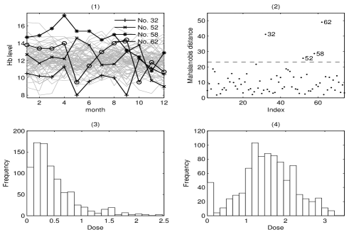
Figure 1: Renal data: (1) the Hb levels for the 74 patients; (2) Mahalanobis distance under the GPFR model; (3) Histogram of dose values before transformation; (4) Histogram of dose values after transformation.

3.1 The population-average inferences

Table 1 reports the MLEs of coefficients for the marginal mean and their standard errors (the first value in parentheses). Here ‘N’ stands for the GPFR model. The degree parameters for three heavy-tailed models are estimated together with other parameters. In Table 1, the negative coefficient of $t$ means that the patients have a decreasing trend in the level of Hb over time without considering dose effects. Note that the values of Bayesian information criterion (BIC) (Schwarz, 1978) and the values of standard errors (the second values of each covariate in fixed-effects) for three heavy-tailed models are often smaller than those for the GPFR model, and the model using T-process (TPFR) is the best choice under BIC. We also report the values of root of mean squared error (RMSE) of the predictions for all patients in Table 1. The smaller values of RMSE under three HPFR models confirm the better performance of the heavy-tailed models in fitting the data. The third values of each covariate in fixed-effects in Table 1 are relative change ratios (%) of the estimates after removing the data from four potential outlier patients. We find that the change ratios of estimates under three HPFR models are much smaller than those under the GPFR model, which indicate the robustness in parameter estimation by using the heavy-tailed models.

[b]

Table 1: Parameter estimation of the renal anaemia data.

Model	Degree	BIC	RMSE	Covariates in fixed-effects
				Constant	$t$	$dose_{m}(t-2)$	$dose_{m}^{2}(t-2)$
N	/	2136	0.416	11.500/0.310/-1.4	-0.036/0.022/-32.9	0.863/0.313/-6.1	-0.196/0.103/-22.1
T	$\widehat{\nu}=7.106$	2088	0.393	11.426/0.297/-0.4	-0.035/0.021/-14.7	0.749/0.304/-0.6	-0.097/0.108/  2.8
SL	$\widehat{\nu}=1.723$	2092	0.391	11.451/0.299/-0.5	-0.035/0.021/-15.2	0.746/0.308/ 0.3	-0.106/0.109/  2.9
CN	$\begin{array}[]{c}\widehat{\nu}=0.424\\ \widehat{\gamma}=0.326\end{array}$	2101	0.392	11.464/0.285/-0.6	-0.040/0.020/-17.8	0.744/0.267/-3.3	-0.094/0.099/-11.7

• RMSE: root of mean squared error of the predictions;

• Three values of each covariate in fixed-effects are in turn, the values of estimate, standard error and the relative change ratio of the estimate after removing the outliers.

We plot the marginal mean curve of Hb levels affected by dose in Figure 2 under four models. The solid lines and the dash lines are drawn respectively, based on the complete 74 patients data, and data deleting those from the four patients. For the GPFR model, the level of Hb increases when the dose is less than 0.8 and decreases slowly after it. However, this turning point changes from 0.8 to 1.3 after deleting the data from the four patients. Under all the HPFR models, the marginal mean maintains to increase on the whole interval but the increasing rate reduces slowly at large dosage. This is a more realistic dose-response curve based on the current understanding on the dose-response relation. Compared with GPFR, the curve shapes under three HPFR models have smaller changes after deleting outliers, which implies the robustness of heavy-tailed models for population-average inferences.

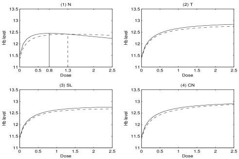
Figure 2: Mean curve of dose response based on original data (Solid line), and data without outliers (Dash line).

3.2 The subject-specific inferences

We now study the patient-specific dose-response curves. We use the data from the first 12 months, and predict (extrapolate) the Hb level at the 14-th month for the dosage from 0 to 2.5. Figure 3 shows the predictions of the patient-specific dose-response curves under the GPFR and TPFR model for two typical patients. For the first patient, the dose-response curve under the GPFR model does not seem realistic, because it cannot achieve the target value of 11.8 even if we increase the dosage. However, the TPFR curve reaches the target when dosage is increased to 1.75. This is the dosage the patient should take at Month 12 if they wants to maintain the Hb level around 11.8 at Month 14. For the second patient, the dose-response curve suggests that the Hb level under the GPFR model reaches the target when dose is 1, and it stays at the same level even when the dosage increases. The TPFR model achieves a more reasonable dose-response relation: the Hb level reaches the target when dose is 0.75 and keep increasing as the dosage increases. We also plotted the PIs for patient-specific curves. Note that the narrowest interval is allocated to the Hb level around the actual dosages the patients took in the previous month. This is because the covariance kernel we used in the stochastic process depends on the difference of dosages between consecutive months, and thus the prediction has less uncertainty in the neighbour of the previous dosage. We will show later how to construct the PIs and show that the proposed PIs maintain the NCLs.

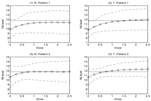
Figure 3: Dose-response of patient-specific prediction for the first selected patient (the upper panel) and the second patient (the lower panel) under the GPFR (N) and TPFR (T) model. The solid lines stand for predictions, and the dash lines are 95% predictive bands.

4 Inference methods

Suppose that we have data from $M$ different subjects, and all functional covariates are observed at points $\boldsymbol{t}_{m}=(t_{m1},\ldots,t_{m,n_{m}})^{\top}$ for the $m$-th subject. Let $\boldsymbol{y}_{m}=(y_{m1},\ldots,y_{m,n_{m}})^{\top}$, $\boldsymbol{V}_{m}$ be the $n_{m}\times p_{v}$ matrix with the $i$-th row $\boldsymbol{v}_{m}^{\top}(t_{mi})$, $\boldsymbol{X}_{m}$ and $\boldsymbol{W}_{m}$ be the matrix defined in the same way as $\boldsymbol{V}_{m}$. Consider the following HPFR model

$$\boldsymbol{y}_{m}=\boldsymbol{\Phi}_{m}\boldsymbol{B}\boldsymbol{u}_{m}+\boldsymbol{V}_{m}\boldsymbol{\gamma}+\boldsymbol{W}_{m}\boldsymbol{b}_{m}+\boldsymbol{\zeta}_{m}+\boldsymbol{\varepsilon}_{m},$$ (5)

where $\boldsymbol{\Phi}_{m}$ is an $n_{m}\times D$ matrix with the $i$-th row $\boldsymbol{\Phi}^{\top}(t_{mi})$, and

$$\begin{split}\boldsymbol{\varepsilon}_{m}|r_{m}&\overset{ind}{\sim}\textup{N}_{n_{m}}(\boldsymbol{0},\kappa(r_{m})\phi_{\varepsilon}\boldsymbol{I}_{n_{m}}),\\ \boldsymbol{b}_{m}|r_{m}&\overset{ind}{\sim}\textup{N}_{p_{w}}(\boldsymbol{0},\kappa(r_{m})\boldsymbol{\Sigma}_{b}),\\ \boldsymbol{\zeta}_{m}|r_{m}&\overset{ind}{\sim}\textup{N}_{n_{m}}(\boldsymbol{0},\kappa(r_{m})\boldsymbol{C}_{m}),\\ r_{m}&\overset{iid}{\sim}\textup{H}(r;\boldsymbol{\nu}),m=1,\ldots,M,\end{split}$$ (6)

$\boldsymbol{C}_{m}$ is an $n_{m}\times n_{m}$ covariance matrix with the $(i,j)$-th element $C(\boldsymbol{x}_{m}(t_{i}),\boldsymbol{x}_{m}(t_{j});\boldsymbol{\theta})$. Then, $\boldsymbol{y}_{m}$ follows a SMN distribution, (Andrews and Mallows, 1974; Fang et al., 1990) i.e., $\textup{SMN}(\boldsymbol{\mu}_{m},\boldsymbol{\Sigma}_{m};\textup{H})$, where $\boldsymbol{\mu}_{m}=\boldsymbol{\Phi}_{m}\boldsymbol{B}\boldsymbol{u}_{m}+\boldsymbol{V}_{m}\boldsymbol{\gamma}$ and $\boldsymbol{\Sigma}_{m}=\boldsymbol{C}_{m}+\boldsymbol{W}_{m}\boldsymbol{\Sigma}_{b}\boldsymbol{W}_{m}^{\top}+\phi_{\varepsilon}\boldsymbol{I}_{n_{m}}$.

4.1 Parameter estimation

Denote the parameter set $\{\boldsymbol{B},\boldsymbol{\gamma},\boldsymbol{\theta},\boldsymbol{\phi}_{b},\phi_{\varepsilon},\boldsymbol{\nu}\}$ by $\boldsymbol{\Theta}$. Let $\boldsymbol{\mathcal{D}}_{c}=\{\boldsymbol{\mathcal{D}}_{m},r_{m},m=1,\ldots,M\}$ be the complete data, where $\boldsymbol{\mathcal{D}}_{m}=\{\boldsymbol{y}_{m},\boldsymbol{u}_{m},\boldsymbol{V}_{m},\boldsymbol{W}_{m},\boldsymbol{X}_{m},\boldsymbol{t}_{m}\}$ be the observed data of the $m$-th subject. For convenience, we separate $\boldsymbol{\Theta}$ into $\boldsymbol{\beta}=(\textup{Vec}(\boldsymbol{B})^{\top},\boldsymbol{\gamma}^{\top})^{\top}$, $\boldsymbol{\psi}=(\boldsymbol{\theta}^{\top},\boldsymbol{\phi}_{b}^{\top},\phi_{\varepsilon})^{\top}$ and $\boldsymbol{\nu}$, where $\boldsymbol{\nu}$ is a parameter for the degree of freedom.

The log-likelihood of the complete data is given by

$$\begin{split}l(\boldsymbol{\Theta}|\boldsymbol{\mathcal{D}}_{c})=&-\frac{1}{2}\sum_{m=1}^{M}\log|\boldsymbol{\Sigma}_{m}|-\frac{1}{2}\sum_{m=1}^{M}n_{m}\log\kappa(r_{m})+\sum_{m=1}^{M}\log h(r_{m};\boldsymbol{\nu})\\ &-\frac{1}{2}\sum_{m=1}^{M}\kappa^{-1}(r_{m})(\boldsymbol{y}_{m}-\boldsymbol{A}_{m}\boldsymbol{\beta})^{\top}\boldsymbol{\Sigma}_{m}^{-1}(\boldsymbol{y}_{m}-\boldsymbol{A}_{m}\boldsymbol{\beta}),\end{split}$$ (7)

where $\boldsymbol{A}_{m}=[\boldsymbol{u}_{m}^{\top}\otimes\boldsymbol{\Phi}_{m},\boldsymbol{V}_{m}]$ satisfies $\boldsymbol{\mu}_{m}=\boldsymbol{A}_{m}\boldsymbol{\beta}$. For the MLEs of $\boldsymbol{\Theta}$, we propose to use an EM algorithm below.

E-step: Given the current value of $\boldsymbol{\Theta}^{(k)}$, we calculate the $Q$-function
$\textup{E}\big{[}l(\boldsymbol{\Theta}|\boldsymbol{\mathcal{D}}_{c})\big{|}\boldsymbol{\Theta}^{(k)},\boldsymbol{\mathcal{D}}_{m},m=1,\ldots,M\big{]}$ which is proportional to

$$Q(\boldsymbol{\Theta}|\boldsymbol{\Theta}^{(k)})=Q_{1}(\boldsymbol{\beta},\boldsymbol{\psi}|\boldsymbol{\Theta}^{(k)})+Q_{2}(\boldsymbol{\nu}|\boldsymbol{\Theta}^{(k)}),$$ (8)

with

$$Q_{1}(\boldsymbol{\beta},\boldsymbol{\psi}|\boldsymbol{\Theta}^{(k)})= -\frac{1}{2}\sum_{m=1}^{M}\log|\boldsymbol{\Sigma}_{m}|-\frac{1}{2}\sum_{m=1}^{M}\pi_{m}^{(k)}(\boldsymbol{y}_{m}-\boldsymbol{A}_{m}\boldsymbol{\beta})^{\top}\boldsymbol{\Sigma}_{m}^{-1}(\boldsymbol{y}_{m}-\boldsymbol{A}_{m}\boldsymbol{\beta}),$$ (9)

$$Q_{2}(\boldsymbol{\nu}|\boldsymbol{\Theta}^{(k)})= \sum_{m=1}^{M}\textup{E}[\log h(r_{m};\boldsymbol{\nu})|\boldsymbol{\Theta}^{(k)},\boldsymbol{\mathcal{D}}_{m}],$$ (10)

where

$$\pi_{m}^{(k)}=\textup{E}[\kappa^{-1}(r_{m})|\boldsymbol{\Theta}^{(k)},\boldsymbol{\mathcal{D}}_{m}].$$ (11)

In the HPs, the weight $\pi_{m}$ is inversely proportional to the Mahalanobis distance $d_{m}=(\boldsymbol{y}_{m}-\boldsymbol{\mu}_{m})^{\top}\boldsymbol{\Sigma}_{m}^{-1}(\boldsymbol{y}_{m}-\boldsymbol{\mu}_{m})$ (see supplementary materials). In the presence of outliers or model misspecification, $d_{m}$ increases, leading to smaller weight to give robust analysis.

The likelihood (7) is the h-likelihood of Lee and Nelder (1996). We can estimate the parameters by using the h-likelihood method. Given $\boldsymbol{\Theta}$, maximizing the conditional likelihood $p_{\boldsymbol{\Theta}}(r_{m}|\boldsymbol{y}_{m})$ with respect to $r_{m}$ is equivalent to maximizing the h-likelihood $L(\boldsymbol{\Theta},r_{m};\boldsymbol{y}_{m},r_{m})$, which has an explicit form as (7). To obtain MLEs of $\boldsymbol{\Theta}$ in h-likelihood approach, the Laplace approximation has been proposed.(Lee et al., 2006) However, the EM algorithm is more efficient in the HPFR model, because the E-step (11) is straightforward. Following ECM (Meng and Rubin, 1993) and ECME,(Liu and Rubin, 1994) we implement the EM algorithm as follows.

CM-step: We maximize (8) with respect to $\boldsymbol{\Theta}$ to get the updated parameter given $\boldsymbol{\Theta}^{(k)}$. We propose the following sub-iterative process:

1. Set the least square estimation of $\boldsymbol{\beta}$ as the initial value $\boldsymbol{\beta}^{(0)}$ under the assumption: $\boldsymbol{\Sigma}_{m}=\boldsymbol{I}_{m}$ and $\pi_{m}=1$ for $m=1,\ldots,M$;

2. Obtain the initial value $\boldsymbol{\psi}^{(0)}$ by maximizing the $Q$-function in equation (9) under $\boldsymbol{\beta}^{(0)}$ and $\pi_{m}=1$;

3. Choose a sensible initial value of $\boldsymbol{\nu}^{(0)}$;

4. Calculate the weights $\pi_{m}$ $(m=1,\ldots,M)$ under the current values $\boldsymbol{\beta}$, $\boldsymbol{\psi}$ and $\boldsymbol{\nu}$;

5. Update $\boldsymbol{\beta}$ under the current values of $\pi_{m}$, $\boldsymbol{\psi}$ by

   $$\boldsymbol{\beta}^{(k+1)}=\big{\{}\sum_{m=1}^{M}\pi_{m}^{(k)}\boldsymbol{A}_{m}^{\top}\boldsymbol{\Sigma}_{m}^{-1}\boldsymbol{A}_{m}\big{\}}^{-1}\big{\{}\sum_{m=1}^{M}\pi_{m}^{(k)}\boldsymbol{A}_{m}^{\top}\boldsymbol{\Sigma}_{m}^{-1}\boldsymbol{y}_{m}\big{\}}\big{|}_{\boldsymbol{\psi}^{(k)}};$$ (12)

6. Update $\boldsymbol{\psi}$ by maximizing the $Q$-function in equation (9) under the current values of $\boldsymbol{\beta}$ and $\pi_{m}$;

7. Given the current values of $\boldsymbol{\beta}$ and $\boldsymbol{\psi}$, update $\boldsymbol{\nu}$ by maximizing the constrained actual marginal log-likelihood function (Liu and Rubin, 1994) of $\{\boldsymbol{y}_{m},m=1,\ldots,M\}$ over $\boldsymbol{\nu}$.

Ideally we need to repeat steps 4 to 7 until it reaches convergence. Practically we can set a threshold and stop the sub-iteration when $\|\boldsymbol{\Theta}^{(k+1)}-\boldsymbol{\Theta}^{(k)}\|$ is smaller than the threshold. Step 6 is analogous to that under GP assumptions by transforming the residual $\boldsymbol{e}_{m}=\boldsymbol{y}_{m}-\boldsymbol{A}_{m}\boldsymbol{\beta}$ into $\widetilde{\boldsymbol{e}}_{m}=\sqrt{\pi_{m}}(\boldsymbol{y}_{m}-\boldsymbol{A}_{m}\boldsymbol{\beta})$. Following the ECME algorithm (Liu and Rubin, 1994), step 7 does not maximize the expected log-likelihood (10) but maximizes the actual log-likelihood over $\boldsymbol{\nu}$, which yields a much faster converging speed. The actual log-likelihood of $\{\boldsymbol{y}_{m},m=1,\ldots,M\}$ as well as the score function of $\boldsymbol{\Theta}$ under some SMN distributions are given in supplementary materials.

The asymptotic confidence intervals of the MLEs for this model can be obtained through the observed information matrix $\mathbf{J}(\widehat{\boldsymbol{\Theta}})$ or the expected information matrix $\mathbf{I}(\widehat{\boldsymbol{\Theta}})$ (see supplementary materials). Here we estimate the degree $\boldsymbol{\nu}$ together with $\boldsymbol{\beta}$ and $\boldsymbol{\psi}$. When sample size is small, the estimation of $\boldsymbol{\nu}$ may be not reliable. In this case, we may fix its value, e.g., choose $\nu=4$ for Student-$t$,(Lange et al., 1989) or choose $\boldsymbol{\nu}$ by BIC or by cross-validation.

4.2 Prediction

Suppose that we want to predict the responses $\boldsymbol{y}^{\ast}=(y_{1}^{\ast},\ldots,y_{n}^{\ast})^{\top}$ of a new $(M+1)$-th subject at points $\boldsymbol{t}^{\ast}=(t_{1}^{\ast},\ldots,t_{n}^{\ast})^{\top}$. Besides the data of $M$ subjects, suppose that we have $n_{M+1}$ observations for the new $(M+1)$-th subject at points $\boldsymbol{t}_{M+1}=(t_{M+1,1},\ldots,t_{M+1,n_{M+1}})^{\top}$. Let $\boldsymbol{\mathcal{D}}_{M+1}=\{\boldsymbol{y}_{M+1},\boldsymbol{u}_{M+1},\boldsymbol{V}_{M+1},\boldsymbol{W}_{M+1},\boldsymbol{X}_{M+1},\boldsymbol{t}_{M+1}\}$ and $\boldsymbol{\mathcal{D}}=\{\boldsymbol{\mathcal{D}}_{m}|m=1,\ldots,M+1\}$ be the observed data.

We rewrite model (5) as

$$\boldsymbol{y}_{m}=\boldsymbol{\mu}_{m}+\widetilde{\boldsymbol{\tau}}_{m},$$ (13)

with $\widetilde{\boldsymbol{\tau}}_{m}\overset{ind}{\sim}\textup{SMN}(\boldsymbol{0},\boldsymbol{\Sigma}_{m};\textup{H})$ for $m=1,\ldots,M+1$. For the $(M+1)$-th subject, let $\widetilde{\boldsymbol{\tau}}^{\ast}$ be the random-effects at unobserved points $\boldsymbol{t}^{\ast}$, while $\widetilde{\boldsymbol{\tau}}_{M+1}$ be the random-effects at observed points $\boldsymbol{t}_{M+1}$. Thus, we have

$${\big{(}\widetilde{\boldsymbol{\tau}}_{M+1}^{\top},\widetilde{\boldsymbol{\tau}}^{\ast\top}\big{)}}^{\top}{\big{|}}r_{M+1}\sim\textup{N}_{n_{M+1}+n}(\boldsymbol{0},\kappa(r_{M+1})\widetilde{\boldsymbol{\Sigma}}_{M+1}),$$ (14)

where

$$\widetilde{\boldsymbol{\Sigma}}_{M+1}=\left(\begin{array}[]{cc}\boldsymbol{\Sigma}_{M+1}&\boldsymbol{\Sigma}_{M+1}^{\ast}\\ \boldsymbol{\Sigma}_{M+1}^{\ast\top}&\boldsymbol{\Sigma}^{\ast}\end{array}\right),$$ (15)

with $\boldsymbol{\Sigma}^{\ast}$ and $\boldsymbol{\Sigma}_{M+1}^{\ast}$ are, respectively, the covariance matrix of the new subject with elements evaluated from the covariance function (2) at point pairs $(t_{j}^{\ast},t_{k}^{\ast})$ and $(t_{i},t_{k}^{\ast})$ for $i\in\{1,\ldots,n_{M+1}\}$ and $j,k\in\{1,\ldots,n\}$. Then, the conditional expectation of $\boldsymbol{y}^{\ast}$ given $\boldsymbol{\mathcal{D}}_{M+1}$ and $\boldsymbol{\Theta}$ is

$$\begin{split}\textup{E}(\boldsymbol{y}^{\ast}|\boldsymbol{\mathcal{D}}_{M+1};\boldsymbol{\Theta})&=\textup{E}(\boldsymbol{\mu}^{\ast}+\widetilde{\boldsymbol{\tau}}^{\ast}|\boldsymbol{\mathcal{D}}_{M+1};\boldsymbol{\Theta})\\ &=\boldsymbol{\mu}^{\ast}+\textup{E}\big{[}\textup{E}(\widetilde{\boldsymbol{\tau}}^{\ast}|r_{M+1},\boldsymbol{\mathcal{D}}_{M+1};\boldsymbol{\Theta})\big{]}\\ &=\boldsymbol{\mu}^{\ast}+\boldsymbol{\Sigma}_{M+1}^{\ast\top}\boldsymbol{\Sigma}_{M+1}^{-1}(\boldsymbol{y}_{M+1}-\boldsymbol{\mu}_{M+1}),\end{split}$$ (16)

where $\boldsymbol{\mu}^{\ast}$ and $\boldsymbol{\mu}_{M+1}$ are respectively the marginal mean curve of the new subject at points $\boldsymbol{t}^{\ast}$ and $\boldsymbol{t}_{M+1}$.

The conditional variance of $\boldsymbol{y}^{\ast}$ given $\boldsymbol{\mathcal{D}}_{M+1}$ and $\boldsymbol{\Theta}$ is given by

$$\begin{split}\textup{Var}(\boldsymbol{y}^{\ast}|\boldsymbol{\mathcal{D}}_{M+1};\boldsymbol{\Theta})&=\textup{E}(\boldsymbol{y}^{\ast}\boldsymbol{y}^{\ast\top}|\boldsymbol{\mathcal{D}}_{M+1};\boldsymbol{\Theta})-\textup{E}(\boldsymbol{y}^{\ast}|\boldsymbol{\mathcal{D}}_{M+1};\boldsymbol{\Theta})\textup{E}(\boldsymbol{y}^{\ast\top}|\boldsymbol{\mathcal{D}}_{M+1};\boldsymbol{\Theta})\\ &=\textup{E}\big{[}\textup{Var}(\boldsymbol{y}^{\ast}|r_{M+1},\boldsymbol{\mathcal{D}}_{M+1};\boldsymbol{\Theta})\big{]}\\ &=\textup{E}[\kappa(r_{M+1})|\boldsymbol{\mathcal{D}}_{M+1};\boldsymbol{\Theta}](\boldsymbol{\Sigma}^{\ast}-\boldsymbol{\Sigma}_{M+1}^{\ast\top}\boldsymbol{\Sigma}_{M+1}^{-1}\boldsymbol{\Sigma}_{M+1}^{\ast}).\end{split}$$ (17)

For GP models, PIs have been studied, assuming normal distribution with the first two moments (16) and (17).(Wang and Shi, 2014) But, the predictive distribution for the conditional mean $p(\boldsymbol{y}^{\ast}|\boldsymbol{\mathcal{D}}_{M+1};\widehat{\boldsymbol{\Theta}})$ under HPFR models may not be normal. For instance the T-process with low degree of freedom, the normal approximation may not be appropriate. Thus, we should compute the quantiles based on the true predictive distribution for a better prediction. However, the resulting PIs would be liberal because they do not take account for the uncertainty in estimation the parameters.(Bjørnstad, 1990, 1996)

We propose the following parametric bootstrap method based on a finite sample adjustment to remedy the drawback:

1. Generate $\boldsymbol{\Theta}_{j}^{\ast}$ $(j=1,\ldots,J)$ from its asymptotic distribution $\textup{N}(\widehat{\boldsymbol{\Theta}},\mathbf{J}^{-1}(\widehat{\boldsymbol{\Theta}}))$;

2. Approximate the predictive distribution of $\boldsymbol{y}^{\ast}$ by

   $$\begin{split}p(\boldsymbol{y}^{\ast}|\boldsymbol{\mathcal{D}})&=\int p(\boldsymbol{y}^{\ast}|\boldsymbol{\mathcal{D}}_{M+1};\widehat{\boldsymbol{\Theta}})p(\widehat{\boldsymbol{\Theta}}|\boldsymbol{\mathcal{D}})\textup{d}\widehat{\boldsymbol{\Theta}}\\ &\approx\frac{1}{J}\sum_{j=1}^{J}p(\boldsymbol{y}^{\ast}|\boldsymbol{\mathcal{D}}_{M+1};\boldsymbol{\Theta}_{j}^{\ast}).\end{split}$$ (18)

Note that Step (2) involves the generation of data from $p(\boldsymbol{y}^{\ast}|\boldsymbol{\mathcal{D}}_{M+1};\boldsymbol{\Theta}_{j}^{\ast})$ which may be not straightforward in some cases. This problem can be addressed by augmenting the latent variable $r_{M+1}$ in the process. We first generate $r_{M+1}$ from the conditional distribution $p(r_{M+1}|\boldsymbol{\mathcal{D}}_{M+1};\boldsymbol{\Theta}_{j}^{\ast})$ which is given in supplementary materials for some distributions. Given $\boldsymbol{\mathcal{D}}_{M+1}$ and $r_{M+1}$, it is straightforward to generate $\boldsymbol{y}^{\ast}$ since its conditional distribution is Gaussian:

$$\boldsymbol{y}^{\ast}|r_{M+1},\boldsymbol{\mathcal{D}}_{M+1},\boldsymbol{\Theta}_{j}^{\ast}\sim\textup{N}_{n}(\widetilde{\boldsymbol{\mu}}^{\ast},\kappa(r_{M+1})\widetilde{\boldsymbol{\Sigma}}^{\ast}),$$ (19)

with $\widetilde{\boldsymbol{\mu}}^{\ast}=\boldsymbol{\mu}^{\ast}+\boldsymbol{\Sigma}_{M+1}^{\ast\top}\boldsymbol{\Sigma}_{M+1}^{-1}(\boldsymbol{y}_{M+1}-\boldsymbol{\mu}_{M+1})$ and $\widetilde{\boldsymbol{\Sigma}}^{\ast}=\boldsymbol{\Sigma}^{\ast}-\boldsymbol{\Sigma}_{M+1}^{\ast\top}\boldsymbol{\Sigma}_{M+1}^{-1}\boldsymbol{\Sigma}_{M+1}^{\ast}$ evaluated at $\boldsymbol{\Theta}_{j}^{\ast}$. Hence, we can obtain the prediction as well as pointwise PIs of $\boldsymbol{y}^{\ast}$ using the sample quantiles calculated from bootstrap replications.

The bootstrap method can also be used to calculate other quantities, such as the subject-specific random-effects. It can be considered as an extension of PIs (Lee and Kim, 2016) for random-effects to curve predictions.

4.3 Information consistency

Seeger et al. (2008) proved information consistency that the prediction based on GP model can be consistent to the true curve, which has been extended to generalized GPFR model (Wang and Shi, 2014) and T-process regression model. (Wang et al., 2016) We now discuss this information consistency for the HPFR model.

For convenience, we omit the subscript $m$ here and denote the data by $\boldsymbol{y}_{n}=(y_{1},\ldots,y_{n})^{\top}$ at points $\boldsymbol{t_{n}}=(t_{1},\ldots,t_{n})^{\top}$ and all the corresponding covariates in the random-effects as $\boldsymbol{X}_{n}=(\boldsymbol{x}_{1},\ldots,\boldsymbol{x}_{n})^{\top}$, where $\boldsymbol{x}_{i}\in\mathcal{X}\subset\mathbb{R}^{p_{x}}$ are independently drawn from a distribution $\mathcal{U}(\boldsymbol{x})$. Let $p(\boldsymbol{y}_{n}|\tau_{0},\boldsymbol{X}_{n})$ be the density function of $\boldsymbol{y}_{n}$ given $\tau_{0}$ and $\boldsymbol{X}_{n}$, where $\tau_{0}(\cdot)$ is the true underling function and hence the true mean of $y_{i}$ is given by $\mu(t_{i})+\tau_{0}(\boldsymbol{x}_{i})$. Let

$$p_{\boldsymbol{\theta}}(\boldsymbol{y}_{n}|\boldsymbol{X}_{n})=\int_{\mathcal{F}}p(\boldsymbol{y}_{n}|\tau,\boldsymbol{X}_{n})\leavevmode\nobreak\ \textup{d}p_{\boldsymbol{\theta}}(\tau)$$

be the density of $\boldsymbol{y}_{n}$ given $\boldsymbol{X}_{n}$ based on the HPFR model, where $p_{\boldsymbol{\theta}}(\tau)$ is a measure of the stochastic process $\tau(\cdot)$ on space $\mathcal{F}=\{\tau(\cdot):\leavevmode\nobreak\ \mathcal{X}\rightarrow\mathbb{R}\}$, and $\boldsymbol{\theta}$ contains all the parameters in the covariance function of $\tau(\cdot)$. Denote $\textup{D}[p_{1},p_{2}]=\int(\log p_{1}-\log p_{2})\leavevmode\nobreak\ \textup{d}p_{1}$ as the Kullback-Leibler divergence between $p_{1}$ and $p_{2}$, we have the following result.

Theorem 1.

Under appropriate conditions:

(C1)

The covariance kernel function $C(\cdot,\cdot;\boldsymbol{\theta})$ is continuous in $\boldsymbol{\theta}$ and $\widehat{\boldsymbol{\theta}}\rightarrow\boldsymbol{\theta}$ almost surely as $n\rightarrow\infty$;

(C2)

The reproducing kernel Hilbert space (RKHS) norm $\|\tau_{0}\|_{c}$ is bounded;

(C3)

The expected regret term $\textup{E}_{\boldsymbol{X}_{n}}(\log|\boldsymbol{I}_{n}+\phi^{-1}\boldsymbol{C}_{n}|)=o(n)$,

we have

$$\frac{1}{n}\textup{E}_{\boldsymbol{X}_{n}}(\textup{D}[p(\boldsymbol{y}_{n}|\tau_{0},\boldsymbol{X}_{n}),\leavevmode\nobreak\ p_{\widehat{\boldsymbol{\theta}}}(\boldsymbol{y}_{n}|\boldsymbol{X}_{n})])\rightarrow 0\quad\text{as}\quad n\rightarrow\infty,$$ (20)

where $p_{\widehat{\boldsymbol{\theta}}}(\boldsymbol{y}_{n}|\boldsymbol{X}_{n})$ is the estimated density of $\boldsymbol{y}_{n}$ under the HPFR model, $\textup{E}_{\boldsymbol{X}_{n}}$ denotes the expectation under the distribution of $\boldsymbol{X}_{n}$.

Proof is in supplementary materials. Note here that $p(\boldsymbol{y}_{n}|\tau_{0},\boldsymbol{X}_{n})$ is the density of the true model and $p_{\widehat{\boldsymbol{\theta}}}(\boldsymbol{y}_{n}|\boldsymbol{X}_{n})$ is that of the working model, and it achieves information consistency, i.e., the density of working model converges to that of true model. The estimation of the mean structure $\mu_{m}(t)$ is based on all independent subjects and has been proved to be consistent in many functional models.(Ramsay and Silverman, 2005; Yao et al., 2005; Li and Hsing, 2010) Under the working model (5) of the observations, the consistency of the estimators $\widehat{\boldsymbol{\Theta}}$ is easily hold since it is essentially an MLE of a longitudinal model. The expected regret term $\textup{E}_{\boldsymbol{X}_{n}}(\log|\boldsymbol{I}_{n}+\phi^{-1}\boldsymbol{C}_{n}|)$ is of order $o(n)$ for some widely used covariance kernels.(Seeger et al., 2008)

5 Simulation studies

We now investigate the performance of the HPFR model in terms of accuracy and robustness for both estimation and prediction. We will compare models with the following three types of process: N (GP), T with $\nu=4$ and SL with $\nu=1.3$.

The mean curve of the true model is $\mu(t)=0.8\sin((0.5t)^{3})$ with $t$ equally distributed in $[-4,4]$. The random terms $\widetilde{\tau}_{m}(t)$’s are generated under a SMGP by setting: $x_{m}(t)=2.5t$ with $\boldsymbol{\theta}^{\top}=(v_{0},w)=(0.04,1)$ for the nonlinear random-effects, $w_{m}(t)=0.5t$ with $\phi_{b}=0.01$ for the linear random-effects, and $\phi_{\varepsilon}=0.01$ for the random error.

To compare the performance of different models, we generate data of twenty independent subjects under one of the following five schemes: (I): GPFR; (II) TPFR with $\nu=4$; (III) GPFR with curve disturbance in the 5-th subject (increase the amplitude of $\mu_{5}(t)$ from 0.8 to 4); (IV) GPFR with outliers in the 10-th subject (jump the region $\{y_{10}(t)|t\in[-1,1]\}$ upward 2 units); (V) Combine III and IV. We then use three models (N, T, SL) to fit the data. We estimate the unknown parameters and then calculate the marginal mean curve and random terms for each subject. The functional coefficients involved in the fixed mean term are approximated by cubic B-splines with 18 knots equally spaced in $[-4,4]$ which is suitable for our simulations. In practice, the number of basis functions can be chosen by BIC or other methods.

5.1 Estimation for population-average inferences

We first study the performances of HPFR models for inferences about the marginal mean $\textup{E}[y(t)]=\mu(t)$. Table 2 reports the RMSE between $\mu(t)$ and $\widehat{\mu}(t)$ for $n_{m}=31$ and $61$ based on fifty replications. Under ‘T’ and ‘SL’ we use the $t$-process and slash process with fixed values of $\nu$, while under ‘T1’ and ‘SL1’ we estimate it as well as other parameters. The results under Scheme I show little difference among three models when the data are generated from the GPFR model. However, if the data are generated from the TPFR model (Scheme II), the GPFR model gives a poor fitting. This indicates that HPFR models provide robust fittings against a misspecification of distribution.

We added two types of outliers respectively in Schemes III and IV and both of them in Scheme V. The results obtained from the HPFR models with heavy-tailed process are much better than the GPFR model, indicating that the HPFR models are robust against outliers. The performances of two HPFR models when $\nu$ is estimated (T1 and SL1) are very close to the models when $\nu$ fixed (T and SL). Moreover, the choice between T and SL is not crucial, since their results are quite similar.

[b]

Table 2: RMSE between true mean curve and its estimation.

Scheme	$n_{m}=31$						$n_{m}=61$
	N	T	T1	SL	SL1		N	T	T1	SL	SL1
I	0.055	0.057	0.055	0.056	0.055		0.053	0.055	0.054	0.054	0.053
II	0.076	0.056	0.056	0.056	0.057		0.073	0.055	0.055	0.056	0.056
III	0.111	0.058	0.058	0.057	0.056		0.105	0.056	0.056	0.056	0.055
IV	0.076	0.059	0.059	0.059	0.059		0.075	0.056	0.056	0.056	0.056
V	0.117	0.057	0.057	0.056	0.055		0.116	0.055	0.055	0.055	0.055

• T and SL: the $t$-process and slash process with fixed degrees;

• T1 and SL1: the $t$-process and slash process with estimated degrees.

Figure 4 shows the estimation of mean curve together with its $95\%$ confidence interval under Scheme V with $n_{m}=61$ when we use the GPFR and TPFR model from one simulated data set. It shows clearly that TPFR achieves a smaller bias and narrow but precise confidence intervals for the marginal means. Asymptotic normality of $\widehat{\mu}(t)$ is well established, so that these confidence intervals will be asymptotically correct.

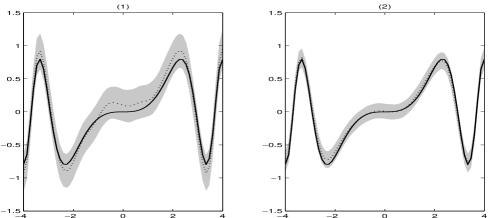
Figure 4: Estimation of mean curve under Scheme V by using: (1) GPFR; (2) TPFR. Solid line: the true mean curve; dotted line: the estimation of the mean curve; shaded area: 95% confidence interval.

5.2 Prediction for subject-specific inferences

We now study inferences about conditional mean, which involves prediction of random-effects $\tau_{m}(t)$ under a conditional model (1).(Lee and Nelder, 2004) Table 3 lists the RMSE between true random-effects $\tau_{m}(t)$ and their predictions $\widehat{\tau}_{m}(t)$ for all subjects under Schemes I and II. Under Schemes III-V, we calculate the RMSE for the subjects except the one with outliers. The RMSEs become smaller for all cases as $n_{m}$ increases. This is because the information about the random-effects is mainly provided by each individual subject and the accuracy is therefore dependent mainly on the sample size of each individual subject. The two HPFR models outperform the GPFR model when the data come from TPFR or GPFR with outliers, which is consistent with the previous findings.

Table 3: RMSE between true random terms and their predictions.

Scheme	$n_{m}=31$				$n_{m}=61$
	N	T	SL		N	T	SL
I	0.084	0.084	0.084		0.073	0.073	0.073
II	0.120	0.113	0.113		0.105	0.092	0.092
III	0.128	0.084	0.084		0.116	0.073	0.072
IV	0.097	0.087	0.086		0.086	0.073	0.073
V	0.140	0.087	0.087		0.126	0.075	0.075

It is important to make interval statements about prediction of individual subject. PIs based on normal assumption with the moments (16) and (17) is called ‘PL0’ (plug-in method with a normal approximation), and those based on quantiles from the predictive distribution $p_{\widehat{\boldsymbol{\Theta}}}(\tau_{m}(t)|\boldsymbol{\mathcal{D}})$ is called ‘PL1’ (plug-in method with the predictive distribution). In this paper, we propose the bootstrap (BTS) PIs in Section 4.3.

We study the PIs for $\tau_{m}(t)$. Table 4 shows the coverage probabilities (CPs) of pointwise PIs for the random terms, and Table 5 shows their average lengths. For BTS, in each replication, we generate 1000 bootstrap samples from the predictive distribution. The value of $J$ in (18) is set as 50, which is big enough to provide a reasonably accurate value to approximate the integration.

[b]

Table 4: CPs (%) of the PIs for random terms.

$n_{m}$	NCL (%)	Scheme	PL0				PL1				BTS
			N	T	SL		N	T	SL		N	T	SL
31	80	I	70.5	71.2	71.1		70.3	70.6	70.5		79.4	80.0	81.5
		II	73.9	70.0	69.9		73.8	69.4	69.4		82.2	78.5	78.1
		V	56.0	68.4	68.5		55.9	67.8	68.0		83.6	79.3	80.5
	90	I	82.1	82.4	82.5		81.9	82.2	82.2		89.4	89.8	90.9
		II	83.9	81.5	81.5		83.8	81.2	81.3		90.6	88.9	88.8
		V	69.3	80.0	80.0		69.1	79.8	79.9		93.6	89.6	90.4
	95	I	88.9	88.9	88.9		88.8	89.0	89.0		94.5	94.8	95.7
		II	89.9	88.0	88.3		89.8	88.2	88.4		94.5	94.2	94.1
		V	78.8	87.3	87.4		78.6	87.4	87.5		97.5	94.7	95.2
61	80	I	64.2	64.5	64.5		64.2	64.3	64.2		78.7	78.7	81.8
		II	66.5	65.4	65.8		66.4	65.1	65.5		80.4	79.1	78.1
		V	45.4	62.5	62.7		45.3	62.2	62.4		83.7	80.3	82.4
	90	I	76.4	76.5	76.6		76.3	76.4	76.4		89.0	88.8	91.4
		II	77.8	77.3	77.5		77.8	77.1	77.4		89.5	89.3	88.5
		V	57.4	74.4	74.5		57.4	74.2	74.3		93.4	90.2	91.5
	95	I	84.1	84.2	84.2		83.9	84.2	84.2		94.1	94.2	95.9
		II	84.9	84.9	85.1		84.8	84.9	85.1		94.0	94.5	94.0
		V	67.0	82.2	82.3		67.0	82.1	82.4		97.4	95.0	95.8

• CP: coverage probabilities; PI: prediction interval; NCL: nominal confidence level;

• PL0: plug-in method with a normal approximation;

• PL1: (plug-in method with the predictive distribution;

• BTS: bootstrap prediction.

Table 5: Lengths of the PIs for random terms.

$n_{m}$	NCL (%)	Scheme	PL0				PL1				BTS
			N	T	SL		N	T	SL		N	T	SL
31	80	I	0.176	0.179	0.178		0.176	0.177	0.176		0.214	0.218	0.226
		II	0.246	0.225	0.225		0.246	0.223	0.223		0.301	0.263	0.261
		V	0.234	0.177	0.176		0.233	0.175	0.174		0.398	0.223	0.227
	90	I	0.225	0.230	0.228		0.225	0.229	0.228		0.275	0.281	0.291
		II	0.316	0.289	0.289		0.316	0.288	0.288		0.386	0.339	0.336
		V	0.300	0.228	0.226		0.300	0.227	0.225		0.510	0.287	0.292
	95	I	0.269	0.274	0.272		0.268	0.275	0.273		0.328	0.336	0.347
		II	0.376	0.344	0.344		0.376	0.346	0.346		0.460	0.405	0.402
		V	0.357	0.271	0.269		0.357	0.273	0.270		0.605	0.343	0.349
61	80	I	0.134	0.136	0.135		0.134	0.135	0.135		0.182	0.184	0.197
		II	0.187	0.170	0.170		0.187	0.169	0.169		0.256	0.216	0.212
		V	0.169	0.134	0.134		0.169	0.133	0.133		0.360	0.196	0.206
	90	I	0.172	0.174	0.174		0.172	0.174	0.174		0.234	0.236	0.253
		II	0.240	0.218	0.218		0.240	0.218	0.217		0.328	0.278	0.272
		V	0.217	0.172	0.172		0.217	0.172	0.171		0.462	0.252	0.265
	95	I	0.205	0.208	0.207		0.205	0.208	0.208		0.278	0.281	0.301
		II	0.286	0.260	0.259		0.286	0.260	0.260		0.390	0.332	0.324
		V	0.258	0.205	0.204		0.258	0.206	0.205		0.549	0.300	0.315

Note that results between PL0 and PL1 are quite similar because a normal approximation may work well in these cases. However, the CPs for both of them are smaller than the nominal confidence levels (NCLs) since they do not take account of the uncertainty in estimating the parameters. We see that the BTS overcomes this drawback and maintains NCLs. When the data are generated from a GPFR model under Scheme I, all three models provide good results and the difference is ignorable. Under Scheme II the data are generated from TPFR model. The advantage of HPFR models is reflected in the precise CPs for both models but have a tighter PI than GPFR (see lengths of PIs of BTS methods from GPFR and HPFR models in Table 5). The data under Scheme II and V are respectively a distribution misspecification and the presence of outliers. We can see the reduction of interval length using HPFR is much bigger under the presence of outliers than a distribution misspecification. The PI becomes wider and the CP is higher than the nominal levels under the GPFR model, while the two HPFR models maintain the robustness advantage reflected in the narrow PIs with precise CPs. This is further illustrated in Figure 5 which exhibits the results for all subjects under Scheme V when $n_{m}=61$ from one simulated data set. It vividly shows that: the BTS-based PIs (dark grey) are slightly wider than the PL-based PIs (light grey), and the TPFR-based PIs (even rows) are narrow but more accurate to cover the true random terms (solid lines) compared with GPFR-based PIs (odd rows).

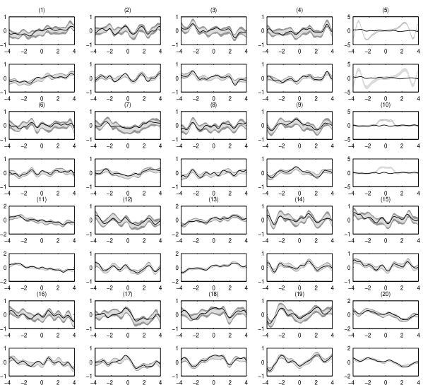
Figure 5: Predictions of all twenty random terms under Scheme V. Odd rows: GPFR-based prediction; Even rows: TPFR-based prediction. Solid line: true underlying random term; Dark grey: $95\%$ BTS-based PI; Light grey: $95\%$ PL1-based PI.

5.3 Prediction for a new subject

We have studied the prediction of subject-specific curves for individuals who are observed. Now, we assess the performance of prediction of $y_{M+1}(t)$ for a new subject. We generate data of twenty one ($M+1$) subjects with $n_{m}=61$ and take the responses from the last (the 21-th) subject as our test target. Here we consider Schemes I, II and V as described before along with a new one: Scheme VI. Under the new scheme the data are generated from GPFR, the same as Scheme I, but with larger random errors in the test subject (increase $\phi_{\varepsilon}$ from 0.01 to 0.05). We use half (30 numbers) of the data from the test subject together with the data from other twenty subjects as observed data, and try to predict the other half (31 numbers) responses (test data) of the test subject. We consider two types of test data: one is randomly chosen, and the other is chosen from the second half, i.e., all the data in $t_{i}\in[0,4]$. They represent respectively interpolation and extrapolation. The later is more challenging than the former. Tables 6-8 give in turn the RMSEs, CPs and lengths of PIs of the BTS-based predictions calculated from fifty replications.

The values of RMSE are reported in Table 6. This can be used to measure the performance of prediction. For interpolation, all three models give very similar results under Schemes I, II and VI, meaning all of them perform pretty well and are robust when the distribution is misspecified. However, the two HPFR models perform more robustly than the GPFR model in the presence of outliers under Scheme V. The results for extrapolation almost tell the same story. Overall the errors for extrapolation are larger than the errors for interpolation.

We report the values of CPs and the length of PIs in Tables 7 and 8. We have some interesting findings here. First of all, all three models give similar results under Scheme I and the values of CP are all close to the nominal level. This shows good robustness for the two HPFR models since the distribution is misspecified for those two models under Scheme I. The CP values of the two HPFR models are still close to the NCLs under Schemes II and V. But the performance of GPFR is very unreliable. For example, the CPs are $88.3\%$ for interpolation and $98.5\%$ for extrapolation when NCL is $80\%$ under Scheme V. For Scheme VI, the PIs under GPFR are quite narrow leading to smaller CPs. For example, the CPs under GPFR are $69.3\%$ for interpolation and $84.9\%$ for extrapolation when NCL is $95\%$. The GPFR model is very sensitive to the possible fluctuation in a new subject. In contrast, the two HPFR models give better results although those two models also suffer from both distribution specification and high fluctuation in the test subject.

[b]

Table 6: RMSE between true responses and their predictions of a new subject.

Scheme	Interpolation				Extrapolation
	N	T	SL		N	T	SL
I	0.138	0.137	0.138		0.242	0.243	0.243
II	0.198	0.197	0.197		0.311	0.305	0.306
V	0.146	0.137	0.137		0.277	0.249	0.249
VI	0.277	0.277	0.277		0.315	0.315	0.316

• Interpolation: the test data is randomly chosen from the new subject;

• Extrapolation: the test data is chosen from the second half of the new subject.

Table 7: CPs (%) of the PIs for responses of a new subject.

NCL (%)	Scheme	Interpolation				Extrapolation
		N	T	SL		N	T	SL
80	I	81.1	80.6	82.1		76.4	77.0	78.4
	II	85.9	79.6	79.9		82.5	80.6	79.8
	V	88.3	79.5	80.7		98.5	79.7	80.4
	VI	49.9	73.9	74.2		65.6	90.5	90.4
90	I	90.0	90.3	90.6		87.5	88.1	88.5
	II	92.3	90.8	90.7		91.0	91.2	90.5
	V	96.1	90.2	90.8		99.7	90.4	91.0
	VI	60.7	84.8	85.4		76.8	96.5	96.6
95	I	94.7	94.5	95.5		92.8	94.0	94.1
	II	94.9	94.9	95.0		94.8	95.7	95.9
	V	98.6	94.6	95.5		99.9	94.8	95.7
	VI	69.3	91.2	91.0		84.9	98.5	98.5

Table 8: Lengths the PIs for responses of a new subject.

NCL (%)	Scheme	Interpolation				Extrapolation
		N	T	SL		N	T	SL
80	I	0.353	0.356	0.365		0.584	0.598	0.606
	II	0.494	0.429	0.428		0.787	0.735	0.729
	V	0.487	0.353	0.359		1.390	0.642	0.650
	VI	0.365	0.623	0.624		0.589	1.100	1.108
90	I	0.453	0.461	0.471		0.750	0.774	0.784
	II	0.634	0.555	0.553		1.010	0.950	0.943
	V	0.625	0.456	0.463		1.787	0.831	0.840
	VI	0.468	0.806	0.809		0.755	1.423	1.435
95	I	0.541	0.554	0.565		0.894	0.929	0.941
	II	0.756	0.667	0.665		1.203	1.142	1.133
	V	0.746	0.548	0.555		2.131	0.998	1.007
	VI	0.558	0.969	0.973		0.900	1.710	1.726

The predictions with a $95\%$ NCL from one simulated data set are plotted in Figure 6 under Scheme V (upper panel) and VI (lower panel) when $n_{m}=61$. For Scheme V, the PIs under the TPFR model (light grey) are narrow than those under the GPFR model (dark grey), which is more significant for extrapolation (upper-right). Bear in mind that the cover probability for the former is more close to the NCL $95\%$ than the latter. For Scheme VI, the PIs under the GPFR model are too narrow to cover a large proportion of observations, leading to a very small cover probability.

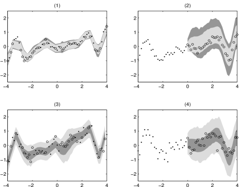
Figure 6: Bootstrap prediction for a new subject. Upper-left: Interpolation under Scheme V; Upper-right: Extrapolation under Scheme VI; Lower-left: Interpolation under Scheme VI; Lower-right: Extrapolation under Scheme VI. Dark grey: $95\%$ BTS-based PI under the GPFR model; Light grey: $95\%$ BTS-based PI under the TPFR model. Dot: true observed response; Circle: true testing response.

Overall, we show that the HPFR models perform better than the GPFR model if the distribution is misspecified and if there are outliers. The proposed BTS based-PIs under HPFR models are quite effective for subject-specific predictions.

6 Concluding remarks and discussion

GP models are widely used for the analysis of medical data. The GPFR model can describe subject-specific characteristics nonparametrically by using a GP via a flexible covariance structure, and can cope with multidimensional covariates in a nonparametric way. However, as we demonstrated in simulation studies, it is sensitive to distribution misspecification and outliers. To overcome this drawback we proposed the HPFR model. We have shown via a comprehensive simulation study that the proposed model has a good property of robustness, giving accurate results when the distribution is misspecified or when the data are contaminated by outliers. The PIs for the subject-specific curves have not been well developed. We propose the use of bootstrap PIs. The simulation study shows that the proposed bootstrap PIs improve existing PIs with respect to the CP and the length of the PI. Computing code of Matlab or R can be provided upon request.

The model has a large flexibility since it includes a class of process regression model for example, the one with a GP,(Shi et al., 2012) the T-process regression model,(Wang et al., 2016) and the model with slash process, mixtures of GP, exponential power process, etc. Even though limited, according to our experience, we prefer the HP model to the GP model because the HP model improves the GP model a lot in the presence of outliers. In complex or big data, identification of all outliers would be difficult. It is reasonable to use the HP model over the GP model since it can bring robust inference and does not lose much efficiency even the data truly comes from GP. As we demonstrated, some criteria, such as the values of BIC, predictive RMSE, standard errors of the estimators and relative change ratios by deleting potential outliers, can be used to select a specific HP model.

All computations were carried out in Matlab 2015b using a 2.4 GHz Inter i5 processor with 8.0 GB RAM. The EM algorithm is very efficient because the E-step is straightforward in our HPFR model. The computation time to achieve convergence is about 12 seconds for each replication of the simulation (Scheme V and $n_{m}=61$) and 6 seconds for the example in Section 3 under the T-process model. However, we can face with the problems from high-dimensional covariates or high frequency data. For high-dimensional covariates, penalized likelihood framework will helpful to select the crucial functional covariates.(Yi et al., 2011) For high frequency data, the HPFR model suffers from massive computation of inverse covariance matrices. A variety of numerical methods, such as Nyström method, active set and filtering approach (Shi and Choi, 2011) may be applied to solve the problem.

One crucial issue in FDA is the modelling of mean function and covariance structure.(Guo, 2002; Antoniadis and Sapatinas, 2007) For the mean function $\mu_{m}(t)$, we used nonparametric function $\boldsymbol{u}_{m}^{\top}\boldsymbol{\beta}(t)$ combined with a parametric (linear) function $\boldsymbol{v}_{m}^{\top}(t)\boldsymbol{\gamma}$. Other mean structures can also be considered. The functional coefficients $\boldsymbol{\beta}(t)$ were approximated by cubic B-splines basis functions under equally spaced knots. It is known that the number of knots tunes the bias and variance of resulting estimator. Thus, the choice of the number of knots is important for the performance of B-spline approximation. The guidance on this issue can be seen in Wu and Zhang (2006). In practice, the number of knots can be determined by generalized cross-validation or BIC methods. However, it is time consuming for high-dimensional and big data. Some low-rank smoothing methods, such as penalized spline smoothing (Ruppert et al., 2003) can be used to decrease the computational burden. For the covariance structure, we combined a parametric (linear) random-effects model $\boldsymbol{w}_{m}^{\top}(t)\boldsymbol{b}_{m}$ with a nonparametric (non-linear) random-effects $\zeta_{m}(\boldsymbol{x}_{m}(t))$ by using HPs. The parametric random-effects model $\boldsymbol{w}_{m}^{\top}(t)\boldsymbol{b}_{m}$ can provide explanatory information between the response and some covariates and characterize the heterogeneity among subjects. A diagonal matrix of $\boldsymbol{\Sigma}_{b}$ means that a few latent variables act independently in subjects, while a non-diagonal positive matrix of $\boldsymbol{\Sigma}_{b}$ implies that there are correlations among the latent variables. The nonparametric process-based random-effects $\zeta_{m}(\boldsymbol{x}_{m}(t))$ can handle flexible subject-specific deviations. The covariance kernel allows us consider multi-dimensional functional covariates to catch up the nonlinear serial correlation within subject. The kernel may represent some symmetric (mirror) effects over time if we only consider time in the process. More discussion of the covariance kernel can be seen in Rasmussen and Williams (2006) and Shi and Choi (2011).

Model diagnosis is also an important issue in FDA. Our HPFR model side-steps the problem of heterogeneity, which means that different subjects share the same location parameters, scale parameters and also the degrees. However, this assumption is doubtful when the data are collected from different groups or sources. Recently, Fang et al. (2016) proposed two tests for evaluating the variance homogeneity in mixed-effects models. Their approaches may also be adapted in the FDA models. For discussion of model-checking plots of various model-misspecification, see Lee et al. (2006). We will develop a model-based method of clustering or classification as a next work if the assumption of homogeneity does not hold.

Acknowledgement

The authors thank Prof. West for providing us the renal anaemia data. The authors are grateful to the Editor, the Associate Editor and two referees, whose questions and insightful comments have greatly improved the work.

The author(s) disclosed receipt of the following financial support for the research, authorship, and/or publication of this article: Dr Cao’s work was supported by the National Science Foundation of China (Grant No. 11301278) and the MOE (Ministry of Education in China) Project of Humanities and Social Sciences (Grant No. 13YJC910001).

Technical details on the conditional distribution properties of SMN distributions, the information matrix and the proof of information consistency are presented in an additional document, which is distributed with the paper as Supplementary Material.

References

- Rasmussen and Williams (2006) Rasmussen CE and Williams CKI. Gaussian Processes for Machine Learning. Cambridge, MA: MIT Press, 2006.
- Shi et al. (2007) Shi JQ, Wang B, Murray-Smith R, et al. Gaussian process functional regression modelling for batch data. Biometrics 2007; 63(3): 714-723.
- Shi et al. (2012) Shi JQ, Wang B, Will EJ, et al. Mixed-effects GPFR models with application to dose-response curve prediction. Stat Med 2012; 31(26): 3165-3177.
- Gramacy and Lian (2012) Gramacy R and Lian H. Gaussian process single-index models as emulators for computer experiments. Technometrics 2012; 54(1): 30-41.
- Wang and Shi (2014) Wang B and Shi JQ. Generalized Gaussian process regression model for non-Gaussian functional Data. J AM Stat Assoc 2014; 109(507): 1123-1133.
- Andrews and Mallows (1974) Andrews DF and Mallows CL. Scale mixtures of normal distributions. J R Soc Series B Stat Methodol 1974; 36(1): 99-102.
- Lachos et al. (2011) Lachos VH, Bandyopadhyay D and Dey DK. Linear and nonlinear mixed-effects models for censored HIV viral loads using normal/independent distributions. Biometrics 2011; 67(4); 1594-1604.
- Meza et al. (2012) Meza C, Osorio F and Cruz R. Estimation in nonlinear mixed-effects models using heavy-tailed distributions. Stat Comput 2012; 22(1): 121-139.
- Cao et al. (2015) Cao CZ, Lin JG., Shi JQ, et al. Multivariate measurement error models for replicated data under heavy-tailed distributions. J Chemometr 2015; 29(8): 457-466.
- Blas et al. (2016) Blas B, Bolfarine H and Lachos VH. Heavy tailed calibration model with Berkson measurement errors for replicated data. Chemometr Intell Lab 2016; 156: 21-35.
- Zhu et al. (2011) Zhu H, Brown PJ and Morris JS. Robust, adaptive functional regression in functional mixed model framework. J AM Stat Assoc 2011; 106(495): 1167-1179.
- Osorio (2016) Osorio F. Influence diagnostics for robust P-splines using scale mixture of normal distributions. Ann I of Stat Math 2016; 68(3): 589-619.
- Lee et al. (2006) Lee Y, Nelder JA and Pawitan Y. Generalized linear models with random-effects, unified analysis via H-likelihood. London: Chapman and Hall, 2006.
- McCulloch and Neuhaus (2011) McCulloch CE and Neuhaus JM. Prediction of random effects in linear and generalized linear models under model misspecification. Biometrics 2011; 67(1): 270-279.
- Lee and Kim (2016) Lee Y and Kim G. H-likelihood predictive intervals for unobservables. Int Stat Rev 2016; Online.
- Diggle et al. (1996) Diggle PJ, Liang KY and Zeger SL. Analysis of longitudinal data. New York: Oxford Univ. Press, 1996.
- Lee and Nelder (2004) Lee Y and Nelder JA. Conditional and marginal models: Another view (with discussion). Stat Sci 2004; 19(2): 219-238.
- Ramsay and Silverman (2005) Ramsay JO and Silverman BW. Functional data analysis, 2nd edn. New York: Springer, 2005.
- Shi and Choi (2011) Shi JQ and Choi T. Gaussian process regression analysis for functional data. London: Chapman and Hall, 2011.