Exfoliation of Graphene and Fluorographene in Molecular and Ionic Liquids

Abstract

We use molecular dynamics simulation to study the exfoliation of graphene and fluorographene in molecular and ionic liquids, by performing computer experiments in which one layer of the 2D nanomaterial is peeled from a stack, in vacuum and in the presence of solvent. The liquid media and the nanomaterials are represented by fully flexible, atomistic force fields. From these simulations we calculate the potential of mean force, or reversible work, required to exfoliate the materials. Calculations in water and organic liquids showed that small amides (NMP, DMF) are among the best solvents for exfoliation, in agreement with experiment. We tested ionic liquids with different cation and anion structures, allowing us to learn about their solvent quality for exfoliation of the nanomaterials. First, a long alkyl side chain on the cation is favourable for exfoliation of both graphene and fluorographene. The presence of aromatic groups on the cation is also favourable for graphene. No beneficial effect was found between fluorine-containing anions and fluorographene. We also analysed the ordering of ions in the interfacial layers with the materials. Near graphene, nonpolar groups are found but also charged groups, whereas near fluorographene almost exclusively non-charged groups are found, with ionic moieties segregated to second layer. Therefore, fluorographene appears as a more hydrophobic surface, as expected.

I Introduction

Two-dimensional (2D) nanomaterials are at the forefront of fundamental and applied research today Ferrari et al. (2015). Among the remarkable features of 2D materials are their electronic structures: graphene Novoselov et al. (2004) is a conductor; h-BN Novoselov et al. (2005) and fluorographene Nair et al. (2010) are insulators; MoS2, other related transition-metal dichalcogenides (TMDC) and phosphorene are semiconductors Wang et al. (2012). Assembling stacks of different 2D materials Gao et al. (2012); Geim and Grigorieva (2013); Novoselov et al. (2016) according to their function (as conductors, insulators or semiconductors) allows fabrication of transistors, capacitors, sensors or optoelectronic devices down to the thickness of atoms Lembke et al. (2015). By relying on delicate noncovalent forces to provide contacts and cohesion, the intrinsic properties of the component materials are largely preserved (although there are junction effects). The ways in which the layers assemble to form 2D heterostructures depends therefore on noncovalent forces between unlike 2D materials, which are not well described or understood at a fundamental level.

Liquid-phase exfoliation is one of the most promissing routes for the production of 2D materials in large scale Nicolosi et al. (2013). Inks of suspended 2D materials can be used to print electronic devices Kelly et al. (2017) on a variety of substracts, including flexible and textile supports. The interplay between interlayer and solvation forces in liquid-based preparation routes (inks) is delicate and also not well described at present. The interactions and interfacial layers of molecular and ionic liquids with nanomaterials are important for other fields of application, such as electrolytes for supercapacitors Simon and Gogotsi (2008) or for ionic-liquid gated transistors Fujimoto and Awaga (2013). In these devices the ordering and dynamics of ions in the interfacial layers are essential to design novel devices for energy storage and flexible electronics.

The chemical nature of the basal planes and edges of 2D materials determines the interactions between layers and also those with liquid media. In graphene the extended $\pi$ electron system of $sp^{2}$ carbons is characterised by a high polarisability, so dispersion and induction interactions dominate. The structure of h-BN is similar, only finely patterned by the slightly polar B-N bonds. TMDC such as MoS2 are composed by three layers of atoms, covalently bonded, in which top and bottom layers of chalcogen atoms atoms, e.g. S, sandwich a central layer of metal atoms, e.g.Mo. Thus there are polar bonds in TMDC materials. In fluorographene all C atoms are $sp^{3}$ with polar C-F bonds and the F atoms forming a “hard” shell that leads to weak interactions, as in perfluorocarbons. For different 2D materials the interactions with solvents will be dominated by distinct terms and one objective of the present study is to improve our understanding of how molecular and ionic liquids organise in the interfacial layers with the materials and how they participate in the exfoliation process.

We have been studying the non-covalent interactions of molecular and ionic liquids with nanomaterials, trying to understant from a physical chemistry standpoint what are the key features that determine the best solvents for exfoliation. One of the first ideas was that the cohesive energy densities between the solvent and the material should match Bergin et al. (2009); Coleman (2013), so that liquids with a surface tension close to the surface energy of the material should be the best solvents. This is verified to an extent, although many solvents with the right value of surface tension, or other solubility parameters, prove not to be as good solvents as anticipated. The situation is clearly more complex and our present understanding needs improvement.

Within this context we have studied exfoliation of phosphorene, which is composed of single layers of P atoms in a puckered structure, with each atom bonded to three others. The P atoms are somewhat under-coordinated and there is a degree of covalence between layers Sresht et al. (2015), so phosphorene is not strictly speaking a van der Waals material. We learned that solvents with flat molecules intercalate favourably between the layers during exfoliation. This descriptor related to molecular shape is not captured easily by quantities such as surface tension or solubility parameters. Next we investigated MoS2 Sresht et al. (2017) and learned that the polarity of Mo-S bonds has a negligible effect on the contact angle of water Govind Rajan et al. (2016). These examples show that subtle and sometimes unexpected factors play important roles.

We have also recently studied the solvation of C60 fullerene and fluorinated C60F48 in ionic liquids Szala-Bilnik et al. (2016), aiming to link the chemical structure of the ions with the ability of the ionic liquids to disaggregate and stabilise suspensions of the nanomaterials. The present work is focused on the interactions of molecular and ionic solvents with graphene and fluorographene, aiming to better undertand what are the molecular features, or descriptors, that contribute to a more efficient exfoliation of the 2D nanomaterials. The method used is atomistic molecular simulation with detailed interaction potentials, validated or developed specifically for the materials studied. Classical molecular dynamics is the adequate scale of description for the problem we wish to study, because we need relatively large systems to represent both edges and the basal planes of the 2D nanomaterials, in stacks and peeled monolayers, and we also need a sufficient volume of solvent so that we can represent both the interfacial layers and the bulk liquids. At the same time, we wish to retain details of the interactions and so we avoided coarse graining of the interaction models. Typical snapshots of the simulated systems are shown in Fig. 1.

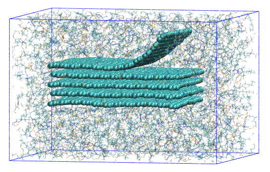
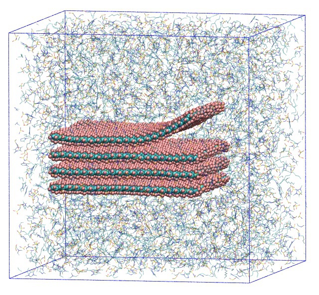
Figure 1: Simulation boxes containing a stack of 2D nanomaterial (graphene and fluorographene) surrounded by solvent. A total of about 40 000 atoms for graphene and 60 000 for fluorographene are simulated for tens of nanoseconds.

Other authors have also looked at ionic liquids as dispersion and exfoliation media for graphene or fullerene using simulation Kamath and Baker (2012); García et al. (2014, 2015); Chaban et al. (2014, 2017), but the interactions or exfoliation of fluorographene have not been extensively studied by computational methods.

The molecular solvents studied here were N-methylpyrrolidone (NMP), dimethylsulfoxide (DMSO), dimethylformamide (DMF) and water (Fig. 2 for molecular structures). They were chosen because of their different interactions and functional groups, with water being small, polar and highly associating through hydrogen bonding, DMSO also polar, and DMF and NMP sharing the amide function but with different molecular sizes. Amides, in particular NMP, are among the most effective solvents to unbundle carbon nanotubes and exfoliate graphene Coleman (2013).

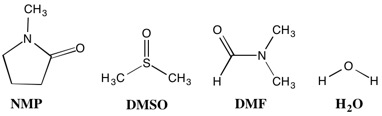
Figure 2: Chemical structures of the molecular solvents.

The ionic liquids selected are based on imidazolium cations haveing different functional groups, associated with different anions. We explored the effect of: i) the length of the alkyl side chain on the imidazolium cations, which determines nonpolar character, by studying alkylmethylimidazolium cations C2C1im+, C4C1im+ and C10C1im+; ii) the head group of the cation, imidazolium or pyrrolidinium in C4C1pyr+, the former being planar and aromatic; and iii) the effect of aromatic benzyl groups on the imidazolium cations, which may enhance the interaction with the extended $\pi$ system of graphene, so we studied bnzmC1im+ and bnzm2im+. The anions varied in size, shape and flexibility, with some being fluorinated and others not. Anions include hexafluorophosphate PF6-, methysulfate C1SO4-, bis(trifluoromethanesulfonyl)amide Ntf2-, thiocyanate SCN-, and tricyanomethanide C(CN)3-. The molecular structures of the ions studied are shown in Fig. 3.

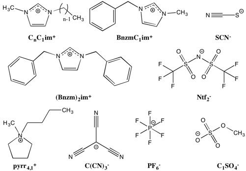
Figure 3: Chemical structures of the cations and anions of the ionic liquids studied here.

II Methods

The structure and interactions of chemical compounds and materials were represented by atomistic force fields, compatible with the OPLS-AA functional form,Jorgensen et al. (1996) e.g. with covalent bonds and valence angles described by harmonic terms, torsion energy profiles by cosine series, and non-bonded interactions by Lennard-Jones sites and atomic partial charges. Parameters for molecular solvents N-methylpyrrolidone (NMP), dimethylsulfoxide (DMSO), dimethylformamide (DMF) were taken from OPLS-AA; water was represented by the SPC/E model Berendsen et al. (1987). Ionic liquids were modelled using the CL&P force field Canongia Lopes et al. (2004); Canongia Lopes and Padua (2012) with ionic charges scaled down to $\pm 0.8e$, which lead to an improved rendering of dynamic and solvation properties Bhargava and Balasubramanian (2007). Graphene and fluorographene sheets (and the non-covalent forces between sheets) were described using OPLS-AA for aromatic Jorgensen and Severance (1990) and perfluorinated molecules Watkins and Jorgensen (2001), respectively. The partial charge scheme of OPLS-AA for aromatic molecules was validated in a previous publication to be a good representation of charge distribution in graphene planes and carbon nanotubes França et al. (2017). Geometric combining rules were used for unlike interactions between graphene or perfluorographene sheets, and also between the molecules or ions of solvent. Between the fluorographene and and the ionic liquids, specific interaction parameters were used Szala-Bilnik et al. (2016).

Initial configurations consisted of a stack of five graphene sheets, or of four fluorographene sheets, placed in periodic parallelepiped boxes using Packmol Martínez et al. (2009) and with the force field generated by the fftool utility Pádua . The dimensions of the stacks are approximately $5.0\text{\,}\mathrm{n}\mathrm{m}$ by $4.0\text{\,}\mathrm{n}\mathrm{m}$ with a thickness of $1.3\text{\,}\mathrm{n}\mathrm{m}$. They are surrounded by sufficient solvent in all directions ($2.0\text{\,}\mathrm{n}\mathrm{m}$ at least, after equilibration) so that periodic images of the stacks do not affect each other, leading to systems made of about 25 000 atoms. Molecular dynamics (MD) trajectories and calculations were carried out using the LAMMPS code Plimpton (1995). The timestep was $1\text{\,}\mathrm{f}\mathrm{s}$, the cutoff for Lennard-Jones interactions $10\text{\,}\mathrm{\SIUnitSymbolAngstrom}$, Coulomb interactions handled using the PPPM method, and H-terminated bonds were constrained using the SHAKE algorithm. Initial configurations were equilibrated at constant temperatures of $350\text{\,}\mathrm{K}$ for molecular solvents and $423\text{\,}\mathrm{K}$ for ionic liquids, and $1\text{\,}\mathrm{b}\mathrm{a}\mathrm{r}$ (regulated by Nosé-Hoover thermostat and barostat) for $1\text{\,}\mathrm{n}\mathrm{s}5\text{\,}\mathrm{n}\mathrm{s}$, respectively. We chose temperatures above ambient to benefit from higher fluidity enabling better sampling and shorter MD runs, especially for the ionic liquids which are relatively viscous. All the molecular solvents considered have their normal boiling points above the chosen temperature.

The reversible work required to peel one layer of nanomaterial from the stack was calculated via the potential of mean foce (PMF). A perpendicular biasing potential of $80\text{\,}\mathrm{k}\mathrm{J}\,\mathrm{m}\mathrm{o}\mathrm{l}^{-1}180\text{\,}\mathrm{k}\mathrm{J}\,\mathrm{m}\mathrm{o}\mathrm{l}^{-1}$ was applied to the top layer of the nanomaterial, evenly distributed over the C atoms of its shorter edge. The C atoms of the edge row of the layer below the top one were tethered by a harmonic potential, and the opposite edge of the top layer was also tethered to avoid sliding. Except for the applied bais and tethers, the rest of the systems evolved freely according to the flexibility of the materials. The coordinate considered in the PMF calculations is the distance $d$ between the centers of mass of the edge row of the top layer and that of the edge of the layer below it. The PMF was calculated using umbrella sampling and the weighed histogram analysis method (WHAM). The coordinate $d$ was sampled between $3.0\text{\,}\mathrm{\SIUnitSymbolAngstrom}16.0\text{\,}\mathrm{\SIUnitSymbolAngstrom}$ for graphene and $5.0\text{\,}\mathrm{\SIUnitSymbolAngstrom}16.0\text{\,}\mathrm{\SIUnitSymbolAngstrom}$ for fluorographene, in steps of $0.5\text{\,}\mathrm{\SIUnitSymbolAngstrom}$, and at each step the system was equilibrated for $80\text{\,}\mathrm{p}\mathrm{s}$ followed by an acquisition period of $120\text{\,}\mathrm{p}\mathrm{s}$. These settings lead to a good sampling and overlap of the coordinate histograms around each $d$ point. An illustration of how the peeling PMF calculation proceeds is shown in Fig. 4.

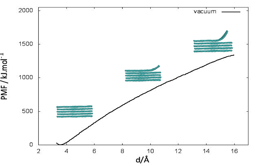
Figure 4: Calculation of the potential of mean force associated with peeling one layer of 2D material from a stack.

The chemical state of the edges of graphene sheets may affect the results, therefore we checked the influence of adding terminal hydrogen atoms to all edges (zig-zag and armchair) of the graphene sheets in our simulations. In fig. 5 we compare graphene with and without H-saturated edges, in terms of the peeling PMF profile, both in vacuum and in one of the ionic liquids studied. No significant difference is seen, therefore we conclude that the present results, obtained with a simple representation without explicit hydrogens, will be valid for H-terminated graphene flakes as well.

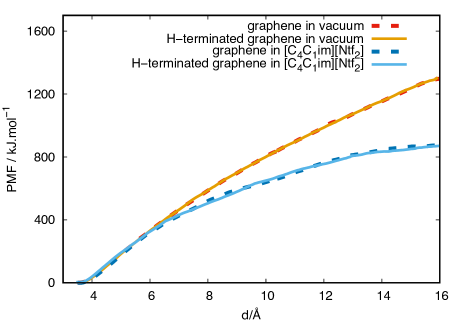
Figure 5: Effect of edge hydrogens on the PMF profile, in vacuum and in [C4C1im][Ntf2] as an example.

The ordering of ions of the different ionic liquids near the surface of the 2D materials was described by axial distribution functions, $g(z)=\rho(z)/\left<\rho\right>$, where $\rho$ is the number density of a specific atom type. These calculations were performed in periodic boxes containing a stack of five layers of graphene or fluorographene, periodic in the $xy$ plane. The simulated systems contained about 20 000 atoms and were equilibrated for $10\text{\,}\mathrm{n}\mathrm{s}$ at $423\text{\,}\mathrm{K}$ and $1\text{\,}\mathrm{b}\mathrm{a}\mathrm{r}$. The axial density profiles were obtained by averaging over 5000 configurations stored during $5\text{\,}\mathrm{n}\mathrm{s}$ runs.

III Results

One of the main quantities reported and analysed in this work is the PMF (free energy) associated with peeling the top layer of 2D material from a stack. The same route is followed in vacuum and in the solvents, so that the effect of the liquids on exfoliation can be compared, between solvents and also with respect to vacuum. The vaccuum calculations provide a measure of the van der Waals forces between layers and account for the bending rigidity of the material. We proceed with the peeling up to a certain separation, beyond which the system enters a steady state beyond which no new information would be obtained. Similar simulations were reported by us in previous studies of exfoliation of other 2D materials, namely phosphorene and MoS2, in which the PMF method used here was set up and validated Sresht et al. (2015, 2017). Besides the PMF calculations, we also analysed the ordering of the ionc liquids in the interfacial layers with the 2D nanomaterials.

III.1 Potential of mean force

The PMF of peeling graphene and fluorographene in the molecular solvents is plotted in Fig. 6. The reversible work required to exfoliate graphene in vacuum is larger than the equivalent quantity for fluorographene: at a separation of $10\text{\,}\mathrm{\SIUnitSymbolAngstrom}$ (counting from the equilibrium inter-layer distance) the PMF is approximately $1150\text{\,}\mathrm{k}\mathrm{J}\,\mathrm{m}\mathrm{o}\mathrm{l}^{-1}$ for graphene and $600\text{\,}\mathrm{k}\mathrm{J}\,\mathrm{m}\mathrm{o}\mathrm{l}^{-1}$ for fluorographene. Thus the “fluorous” interactions between fluorographene sheets are less attractive than between the $\pi$ systems of graphene.

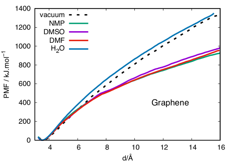
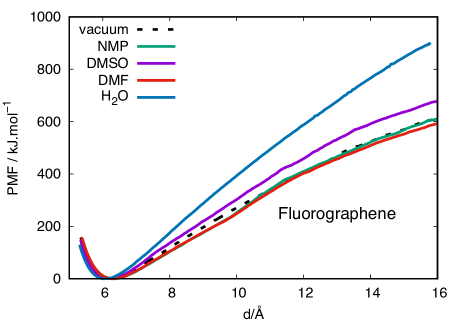
Figure 6: PMF of peeling graphene and fluorographene in molecular solvents at $350\text{\,}\mathrm{K}$.

In liquids PMF curves below the vacuum curve indicate a favourable solvent, whereas curves above the one in vacuum mean that it is more difficult to peel away the top layer in that medium. So, lower curves mean better solvents for exfoliation. For graphene the three organic solvents lead to low PMF values, whereas water follows quite closely the vacuum curve. The PMF values in the three organic solvents are close, but distinguishable, in the order: NMP below (better solvent than) DMF below DMSO below water. These simulation results agree with the experimental order Coleman (2013). Our previous study Szala-Bilnik et al. (2016) revealed easier separation of C60 in organic solvents like DMSO and DMF than in water, in good agreement with the findings for graphene.

For fluorographene in the molecular solvents, PMF values stay close to or above those in vacuum, thus the solvents studied here are not predicted to be good for exfoliating the fluorinated 2D material. Water is clearly the worse, followed by DMSO, with NMP and DMF values cose to those obtained in vacuum. In relative terms, the order between solvents is similar to that obtained for graphene. For smaller fluorinated objects like C60F48 Szala-Bilnik et al. (2016), also neither water nor the organic liquids tested seemed to be good solvents.

The reason why NMP is a better exfoliation medium is is part due to its physical solvent properties, namely that the surface tension matches the surface energy of the material Bergin et al. (2009). This is the argument that “like dissolves like”: the solute-solvent interacton energy should be commensurate with the cohesive energy of the solvent, otherwise one of them will have too strong a tendency to aggregate not favouring the formation of a dispersion. However, this is not the sole descriptor defining a good solvent: the planarity of the amides contributes to an easier intercalation between layers of the 2D material during the exfoliation process Sresht et al. (2015, 2017).

PMF curves obtained in the ionc liquids are shown in Figs. 7 to 8. Similarly to what was obtained in the molecular solvents, PMFs are below the vacuum curve (favourable) for exfoliation of graphene, and above (unfavourable) for flurographene. Different cations lead to quite comparable PMF values, which is an interesting result. It is seen that a longer alkyl chain is beneficial towards exfoliation, both of graphene and fluorograhene. The pyrrolidinium head group is an improvement compared to imidazolium (another interesting result given that imidazolium is aromatic and thus expected to have stronger interactions with graphene). Finally, the presence of one benzyl group is not beneficial towards graphene exfoliation, but two benzyl groups actually lead to the lowest PMF we calcualted. This affinity of the dibenzyl imidazolium cation towards graphene was recently reported experimentally Bari et al. (2014). The best ILs for fluorographene exfoliation among those studied are based on C10C1im+. Also for dissolution of fullerene and fluorinated fullerene Szala-Bilnik et al. (2016), a longer alkyl side chain on the cation was more beneficial than an aromatic group.

Changing the anion leads again to relatively small differences in PMF of peeling graphene, and to more significant differences for fluorographene. A “fluorous” effect was not observed, with C(CN3)- appearing to be a better anion than either PF6- or Ntf2- for exfoliation of fluorographene (Fig. 8).

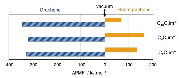
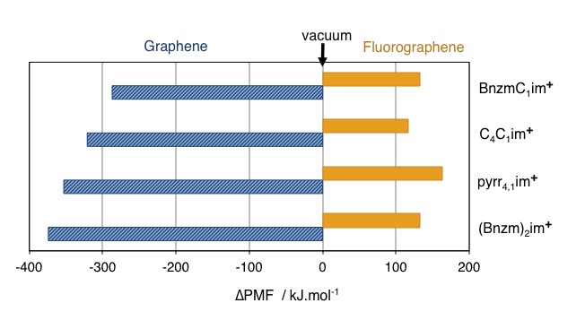
Figure 7: Differences in PMF value of peeling graphene and fluorographene in ionic liquids at $423\text{\,}\mathrm{K}$ to a separation of $10\text{\,}\mathrm{\SIUnitSymbolAngstrom}$, with respect to peeling in vacuum. Effect of alkyl chain or aromatic character of the cation (all ionic liquids have the same Ntf2- anion).

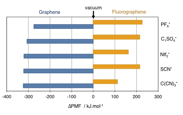
Figure 8: Differences in PMF value of peeling graphene and fluorographene in ionic liquids at $423\text{\,}\mathrm{K}$ to a separation of $10\text{\,}\mathrm{\SIUnitSymbolAngstrom}$, with respect to vacuum. Effect of anion (all ionic liquids have the same C4C1im+ cation).

III.2 Interfacial layering of ionic liquids

The ordering of ions in the interfacial layers with the 2D nanomaterials was assessed through the axial distribution functions of specific atoms of cations and anions, $g(z)=\rho(z)/\left<\rho\right>$, as a function of the distance measured parallel to the surface of the top layer. We present in what follows some $g(z)$ of selected atoms of the ions that allow us to extract what we consider to be significant structural features, avoiding clutter due to the large amount of information available from the MD trajectories.

The first comparison, in Fig. 9, concerns the location of the alkyl chain of [C10C1im][Ntf2] near the surfaces of the materials. It is seen that the terminal C atom of the decyl chain is found adjacent to the surface of both materials, but near the graphene surface are found also atoms of the imidazolium ring and of the anion, whereas the cation headgroup and the anion show no preference for the first interfacial layer with fluorographene. In the interfacial layer with graphene, the C atoms of the imidazolium ring show intense first peaks at the same distance, indicating that the imidazolium rings are oriented parallel to the surface. In the interfacial alyers with fluorographene, the atoms of the cation head-group and of the anion appear in second layer, after the alkyl chains and the F atoms of the anion. Fluorographene appears thus as a more hydrophobic, interacting favourably with the alkyl side chain and the CF3 groups of the anion, but not with the charged moieties. This apparent affinity for fluorine atoms seen in the structural data do not translate into a “fluorous” effect in PMF, as discussed previously.

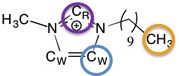
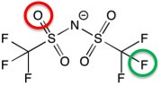
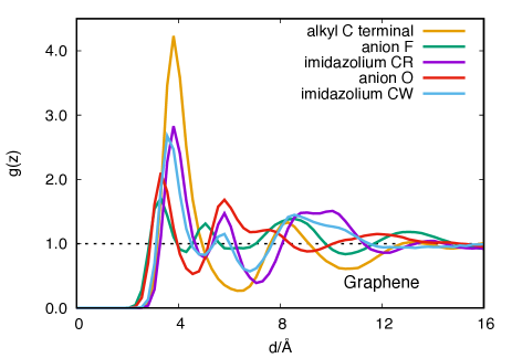
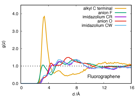
Figure 9: Distribution functions of selected atoms from [C10C1im][Ntf2] as functions of distance $z$ from the surface of graphene and fluorogaphene.

Next we analyse the structural features in the interfacial layers due to the presence of benzyl groups in the imidazolium cations, Fig. 10. We see that the first peak of different C atoms from the benzyl groups (ortho, meta, para) are found at the same distance, indicating that the aromatic rings are preferentially oriented parallel to the surface of the material. The first peaks of the benzyl atoms are more intense and narrow near fluorographene than near graphene. This may be due to the difference in cations, because the imidazolium IL studied near graphene (in terms of $g(z)$) is dibenzyl substituted, whereas the one studied with fluorographene has only one benzyl substituent. As with the alkyl chain discussed previously, in the interfacial layers with graphene, atoms from the imidazolium head-group are found with higher intensity, whereas near fluorographene only the F atoms from the anion show significant presence (besides the benzyl groups). Again, fluorographene leads to more structured interfacial layers, the surface having a stronger hydrophobic character. Contrary to what was observed with the alkyl side chain, in the dibenzylimidazolium IL the cation head-group is not found near the surface of graphene. Integration of the first peaks in the $g(z)$ allows us to know the number of groups in the first interfacial layer. For [bznm2im][Ntf2] near graphene, the area under the first peak is $9.4$ for the aromatic para-C, and for [bznmC1im][Ntf2] the area is $4.3$, or essentially half, meaning that the affinities of the benzyl groups for the two materials seem comparable.

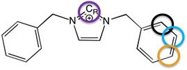
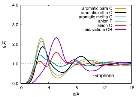
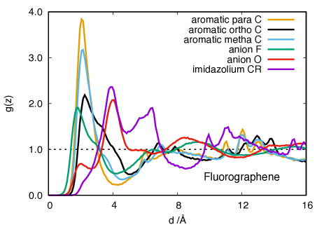
Figure 10: Distribution functions of selected atoms from [bnzm2im][Ntf2] as functions of distance $z$ from the surface of graphene, and of [bnzmC1im][Ntf2] with respect to fluorogaphene.

Finally, we inspect the interfacial ordering of [C4C1im][C(CN)3] near the materials in Fig. 11. It is seen that at the interface with graphene the first peaks coincide, meaning that imidazolium head-groups and side chains, as well as the cyano groups from the anions, are all found in an ordered first layer. At the fluorographene interface the situation is different, with a predominance of terminal C atoms from the butyl side chain of the cation, again indicating the more hydrophobic nature of fluorographene. Also, atoms from the cation head-group and from the anion are found in the interfacial layer, in contrast with what was seen in ionic liquids composed of the Ntf2-.

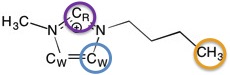
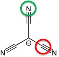
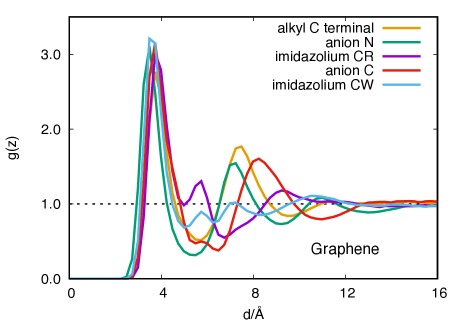
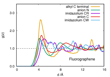
Figure 11: Distribution functions of selected atoms from [C4C1im][C(CN)3] as functions of distance $z$ from the surface of graphene and fluorogaphene.

IV Conclusion

The two types of molecular simulations we performed, to obtain the PMF of peeling away one layer of material and to investigate the ordering of the interfacial layers, provided several pieces of information about molecular and ionic solvents. To start with, attractive forces between layers of graphene are stronger than between those of fluorographene, something that was expected.

Fluorinated graphene appears as a solvophobic material, with which most solvents have low affinity. Graphene, on the other hand, shows affinity for several molecular and ionic liquids, as demonstrated by an easier peeling process in organic solvents such as NMP, and also in ionic liquids with long side chain or aromatic functions. The order of solvents interms of ease of exfoliation obtained here agrees with experiment. Also, the structure at the interfacial layers is different near the two materials: both non-polar side chains and ionic moieties are found near graphene (more polarisable) whereas in the first layer of ionic liquid near fluorographene mostly non-polar side chains are found, with ionic groups displaced to second liquid layer.

In the structural data we could see CF3 groups from anions are found near the surface of fluorographene. However, no such “fluorous” effect was found in the PMF results, with non-halogenated anions such as C(CN)3- proving to be the best for exfoliation. Another aspect of “like dissolves like” that we tested was the effect of aromatic substituent groups in the cations. Dibenzyl imidazolium was found to be a favourable cation for graphene, although not for fluorographene.

Overall, with the families of ionic liquids we studied here, the effect of modifying the cation led to more important changes in PMF than the choice of anion.

V Acknowledgments

This work was supported by the Agence Nationale de la Recherche project CLINT ANR-12-IS10-003.

References

- Ferrari et al. (2015) A. C. Ferrari, F. Bonaccorso, V. Fal’ko, K. S. Novoselov, S. Roche, P. Bøggild, S. Borini, F. H. L. Koppens, V. Palermo, N. Pugno, J. A. Garrido, R. Sordan, A. Bianco, L. Ballerini, M. Prato, E. Lidorikis, J. Kivioja, C. Marinelli, T. Ryhänen, A. Morpurgo, J. N. Coleman, V. Nicolosi, L. Colombo, A. Fert, M. Garcia-Hernandez, A. Bachtold, G. F. Schneider, F. Guinea, C. Dekker, M. Barbone, Z. Sun, C. Galiotis, A. N. Grigorenko, G. Konstantatos, A. Kis, M. Katsnelson, L. Vandersypen, A. Loiseau, V. Morandi, D. Neumaier, E. Treossi, V. Pellegrini, M. Polini, A. Tredicucci, G. M. Williams, B. H. Hong, J.-H. Ahn, J. M. Kim, H. Zirath, B. J. van Wees, H. van der Zant, L. Occhipinti, A. Di Matteo, I. A. Kinloch, T. Seyller, E. Quesnel, X. Feng, K. Teo, N. Rupesinghe, P. Hakonen, S. R. T. Neil, Q. Tannock, T. Löfwander, and J. Kinaret, Nanoscale 7, 4598 (2015).
- Novoselov et al. (2004) K. S. Novoselov, A. K. Geim, S. V. Morozov, D. Jiang, Y. Zhang, S. V. Dubonos, I. V. Grigorieva, and A. A. Firsov, Science 306, 666 (2004).
- Novoselov et al. (2005) K. S. Novoselov, D. Jiang, F. Schedin, T. J. Booth, V. V. Khotkevich, S. V. Morozov, and A. K. Geim, Proc. Nat. Acad. Sci. 102, 10451 (2005).
- Nair et al. (2010) R. R. Nair, W. Ren, R. Jalil, I. Riaz, V. G. Kravets, L. Britnell, P. Blake, F. Schedin, A. S. Mayorov, S. Yuan, M. I. Katsnelson, H.-M. Cheng, W. Strupinski, L. G. Bulusheva, A. V. Okotrub, I. V. Grigorieva, A. N. Grigorenko, K. S. Novoselov, and A. K. Geim, Small 6, 2877 (2010).
- Wang et al. (2012) Q. H. Wang, K. Kalantar-Zadeh, A. Kis, J. N. Coleman, and M. S. Strano, Nature Mat. 7, 699 (2012).
- Gao et al. (2012) G. Gao, W. Gao, E. Cannuccia, J. Taha-Tijerina, L. Balicas, A. Mathkar, T. N. Narayanan, Z. Liu, B. K. Gupta, J. Peng, Y. Yin, A. Rubio, and P. M. Ajayan, Nano Lett. 12, 3518 (2012).
- Geim and Grigorieva (2013) A. K. Geim and I. V. Grigorieva, Nature 499, 419 (2013).
- Novoselov et al. (2016) K. S. Novoselov, A. Mishchenko, A. Carvalho, and A. H. Castro Neto, Science 353, aac9439 (2016).
- Lembke et al. (2015) D. Lembke, S. Bertolazzi, and A. Kis, Acc. Chem. Res. 48, 100 (2015).
- Nicolosi et al. (2013) V. Nicolosi, M. Chhowalla, M. G. Kanatzidis, M. S. Strano, and J. N. Coleman, Science 340, 1226419 (2013).
- Kelly et al. (2017) A. G. Kelly, T. Hallam, C. Backes, A. Harvey, A. S. Esmaeily, I. Godwin, J. Coelho, V. Nicolosi, J. Lauth, A. Kulkarni, S. Kinge, L. D. A. Siebbeles, G. S. Duesberg, and J. N. Coleman, Science 356, 69 (2017).
- Simon and Gogotsi (2008) P. Simon and Y. Gogotsi, Nature Materials 7, 845 (2008).
- Fujimoto and Awaga (2013) T. Fujimoto and K. Awaga, PCCP 15, 8983 (2013).
- Bergin et al. (2009) S. D. Bergin, Z. Sun, D. Rickard, P. V. Streich, J. P. Hamilton, and J. N. Coleman, ACS Nano 3, 2340 (2009).
- Coleman (2013) J. N. Coleman, Acc. Chem. Res. 46, 14 (2013).
- Sresht et al. (2015) V. Sresht, A. A. H. Padua, and D. Blankschtein, ACS Nano 9, 8255 (2015).
- Sresht et al. (2017) V. Sresht, A. Govind Rajan, E. Bordes, M. S. Strano, A. A. H. Padua, and D. Blankschtein, J. Phys. Chem. C , acs.jpcc.7b00484 (2017).
- Govind Rajan et al. (2016) A. Govind Rajan, V. Sresht, A. A. H. Padua, M. S. Strano, and D. Blankschtein, ACS Nano 10, 9145 (2016).
- Szala-Bilnik et al. (2016) J. Szala-Bilnik, M. F. Costa Gomes, and A. A. H. Padua, J. Phys. Chem. C 120, 19396 (2016).
- Kamath and Baker (2012) G. Kamath and G. A. Baker, PCCP 14, 7929 (2012).
- García et al. (2014) G. García, M. Atilhan, and S. Aparicio, J. Phys. Chem. B 118, 11330 (2014).
- García et al. (2015) G. García, M. Atilhan, and S. Aparicio, J. Phys. Chem. B 119, 12224 (2015).
- Chaban et al. (2014) V. V. Chaban, C. Maciel, and E. E. Fileti, J. Sol. Chem. (2014), Chaban:2014do.
- Chaban et al. (2017) V. V. Chaban, E. E. Fileti, and O. V. Prezhdo, J. Phys. Chem. C 121, 911 (2017).
- Jorgensen et al. (1996) W. L. Jorgensen, D. S. Maxwell, and J. Tirado-Rives, J. Am. Chem. Soc. 118, 11225 (1996).
- Berendsen et al. (1987) H. J. C. Berendsen, J. R. Grigera, and T. P. Straatsma, J. Phys. Chem. 91, 6269 (1987).
- Canongia Lopes et al. (2004) J. N. Canongia Lopes, J. Deschamps, and A. A. H. Padua, J. Phys. Chem. B 108, 2038 (2004).
- Canongia Lopes and Padua (2012) J. N. Canongia Lopes and A. A. H. Padua, Theo. Chem. Acc. 131, 1129 (2012).
- Bhargava and Balasubramanian (2007) B. L. Bhargava and S. Balasubramanian, J. Chem. Phys. 127, 114510 (2007).
- Jorgensen and Severance (1990) W. L. Jorgensen and D. L. Severance, J. Am. Chem. Soc. 112, 4768 (1990).
- Watkins and Jorgensen (2001) E. K. Watkins and W. L. Jorgensen, J. Phys. Chem. A 105, 4118 (2001).
- França et al. (2017) J. M. P. França, C. A. Nieto de Castro, and A. A. H. Pádua, PCCP (2017).
- Martínez et al. (2009) L. Martínez, R. Andrade, E. G. Birgin, and J. M. Martínez, J. Comput. Chem. 30, 2157 (2009).
- (34) A. A. H. Pádua, “github.com/agiliopadua/fftool,” .
- Plimpton (1995) S. J. Plimpton, J. Comput. Phys. 117, 1 (1995).
- Bari et al. (2014) R. Bari, G. Tamas, F. Irin, A. J. A. Aquino, M. J. Green, and E. L. Quitevis, Coll. Surf. A 463, 63 (2014).