The Impact of Alternation

Abstract

Alternating automata have been widely used to model and verify systems that handle data from finite domains, such as communication protocols or hardware. The main advantage of the alternating model of computation is that complementation is possible in linear time, thus allowing to concisely encode trace inclusion problems that occur often in verification. In this paper we consider alternating automata over infinite alphabets, whose transition rules are formulae in a combined theory of booleans and some infinite data domain, that relate past and current values of the data variables. The data theory is not fixed, but rather it is a parameter of the class. We show that union, intersection and complementation are possible in linear time in this model and, though the emptiness problem is undecidable, we provide two efficient semi-algorithms, inspired by two state-of-the-art abstraction refinement model checking methods: lazy predicate abstraction [8] and the Impact  semi-algorithm [15]. We have implemented both methods and report the results of an experimental comparison.

I Introduction

The language inclusion problem is recognized as being central to verification of hardware, communication protocols and software systems. A property is a specification of the correct executions of a system, given as a set $\mathcal{P}$ of executions, and the verification problem asks if the set $\mathcal{S}$ of executions of the system under consideration is contained within $\mathcal{P}$.

This problem is at the core of widespread verification techniques, such as automata-theoretic model checking [21], where systems are specified as finite-state automata and properties defined using Linear Temporal Logic [19]. However the bottleneck of this and other related verification techniques is the intractability of language inclusion (PSPACE-complete for finite-state automata on finite words over finite alphabets).

Alternation [3] was introduced as a generalization of nondeterminism, introducing universal, in addition to existential transitions. For automata over finite alphabets, the language inclusion problem can be encoded as the emptiness problem of an alternating automaton of linear size. Moreover, efficient exploration techniques based on antichains are shown to perform well for alternating automata over finite alphabets [5].

Using finite alphabets for the specification of properties and models is however very restrictive, when dealing with real-life computer systems, mostly because of the following reasons. On one hand, programs handle data from very large domains, that can be assumed to be infinite (64-bit integers, floating point numbers, strings of characters, etc.) and their correctness must be specified in terms of the data values. On the other hand, systems must respond to strict deadlines, which requires temporal specifications as timed languages [1].

Although being convenient specification tools, automata over infinite alphabets lack the decidability properties ensured by finite alphabets. In general, when considering infinite data as part of the input alphabet, language inclusion is undecidable and, even complementation becomes impossible, for instance, for timed automata [1] or finite-memory register automata [12]. In some cases, one can recover theoretical decidability, by restricting the number of variables (clocks) in timed automata to one [18], or forbidding relations between current and past/future values, as with symbolic automata [22]. In such cases, the emptiness problem for the alternating versions becomes decidable [13, 4].

In this paper, we present a new model of alternating automata over infinite alphabets consisting of pairs $(a,\nu)$ where $a$ is an input event from a finite set and $\nu$ is a valuation of a finite set $\mathbf{x}$ of variables that range over an infinite domain. We assume that, at all times, the successive values taken by the variables in $\mathbf{x}$ are an observable part of the language, in other words, there are no hidden variables in our model. The transition rules are specified by a set of formulae, in a combined first-order theory of boolean control states and data, that relate past with present values of the variables. We do not fix the data theory a priori, but rather consider it to be a parameter of the class.

A run over an input word $(a_{1},\nu_{1})\ldots(a_{n},\nu_{n})$ is a sequence $\phi_{0}(\mathbf{x}_{0})\Rightarrow\phi_{1}(\mathbf{x}_{0},\mathbf{x}_{1})\Rightarrow\ldots\Rightarrow\phi_{n}(\mathbf{x}_{0},\ldots,\mathbf{x}_{n})$ of rewritings of the initial formula by substituting boolean states with time-stamped transition rules. The word is accepted if the final formula $\phi_{n}(\mathbf{x}_{0},\ldots,\mathbf{x}_{n})$ holds, when all time-stamped variables $\mathbf{x}_{1},\ldots,\mathbf{x}_{n}$ are substituted by their values in $\nu_{1},\ldots,\nu_{n}$, all non-final states replaced by false and all final states by true.

The boolean operations of union, intersection and complement can be implemented in linear time in this model, thus matching the complexity of performing these operations in the finite-alphabet case. The price to be paid is that emptiness becomes undecidable, for which reason we provide two efficient semi-algorithms for emptiness, based on lazy predicate abstraction [8] and the Impact method [15]. These algorithms are proven to terminate and return a word from the language of the automaton, if one exists, but termination is not guaranteed when the language is empty.

We have implemented the boolean operations and emptiness checking semi-algorithms and carried out experiments with examples taken from array logics [2], timed automata [9], communication protocols [23] and hardware verification [20].

Related Work

Data languages and automata have been defined previously, in a classical nondeterministic setting. For instance, Kaminski and Francez [12] consider languages, over an infinite alphabet of data, recognized by automata with a finite number of registers, that store the input data and compare it using equality. Just as the timed languages recognized by timed automata [1], these languages, called quasi-regular, are not closed under complement, but their emptiness is decidable. The impossibility of complementation here is caused by the use of hidden variables, which we do not allow. Emptiness is however undecidable in our case, mainly because counting (incrementing and comparing to a constant) data values is allowed, in many data theories.

Another related model is that of predicate automata [6], which recognize languages over integer data by labeling the words with conjunctions of uninterpreted predicates. We intend to explore further the connection with our model of alternating data automata, in order to apply our method to the verification of parallel programs.

The model presented in this paper stems from the language inclusion problem considered in [11]. There we provide a semi-algorithm for inclusion of data languages, based on an exponential determinization procedure and an abstraction refinement loop using lazy predicate abstraction [8]. In this work we consider the full model of alternation and rely entirely on the ability of SMT solvers to produce interpolants in the combined theory of booleans and data. Since determinisation is not needed and complementation is possible in linear time, the bulk of the work is carried out by the decision procedure.

The emptiness check for alternating data automata adapts similar semi-algorithms for nondeterministic infinite-state programs to the alternating model of computation. In particular, we considered the state-of-the-art Impact  procedure [15] that is shown to outperform lazy predicate abstraction [8] in the nondeterministic case, and generalized it to cope with alternation. More recent approaches for interpolant-based abstraction refinement target Horn systems [16, 10], used to encode recursive and concurrent programs [7]. However, the emptiness of alternating word automata cannot be directly encoded using Horn clauses, because all the branches of the computation synchronize on the same input, which cannot be encoded by a finite number of local (equality) constraints. We believe that the lazy annotation techniques for Horn clauses are suited for branching computations, which we intend to consider in a future tree automata setting.

II Preliminaries

A signature $\mathsf{S}=(\mathsf{S}^{\mathrm{s}},\mathsf{S}^{\mathrm{f}})$ consists of a set $\mathsf{S}^{\mathrm{s}}$ of sort symbols and a set $\mathsf{S}^{\mathrm{f}}$ of sorted function symbols. To simplify the presentation, we assume w.l.o.g. that $\mathsf{S}^{\mathrm{s}}=\left\{\mathsf{Data},\mathsf{Bool}\right\}$ and each function symbol $f\in\mathsf{S}^{\mathrm{f}}$ has $\#(f)\geq 0$ arguments of sort $\mathsf{Data}$ and return value $\sigma(f)\in\mathsf{S}^{\mathrm{s}}$. If $\#(f)=0$ then $f$ is a constant. We consider the constants $\top$ and $\bot$ of sort $\mathsf{Bool}$.

We consider an infinite countable set of variables $\mathsf{Var}$, where each $x\in\mathsf{Var}$ has an associated sort $\sigma(x)$. A term $t$ of sort $\sigma(t)=S$ is a variable $x\in\mathsf{Var}$ where $\sigma(x)=S$, or $f(t_{1},\ldots,t_{\#(f)})$ where $t_{1},\ldots,t_{\#(f)}$ are terms of sort $\mathsf{Data}$ and $\sigma(f)=S$. An atom is a term of sort $\mathsf{Bool}$ or an equality $t\approx s$ between two terms of sort $\mathsf{Data}$. A formula is an existentially quantified combination of atoms using disjunction $\vee$, conjunction $\wedge$ and negation $\neg$ and we write $\phi\rightarrow\psi$ for $\neg\phi\vee\psi$.

We denote by $\mathrm{FV}^{\sigma}(\phi)$ the set of free variables of sort $\sigma$ in $\phi$ and write $\mathrm{FV}(\phi)$ for $\bigcup_{\sigma\in\mathsf{S}^{\mathrm{s}}}\mathrm{FV}^{\sigma}(\phi)$. For a variable $x\in\mathrm{FV}(\phi)$ and a term $t$ such that $\sigma(t)=\sigma(x)$, let $\phi[t/x]$ be the result of replacing each occurrence of $x$ by $t$. For indexed sets $\mathbf{t}=\left\{t_{1},\ldots,t_{n}\right\}$ and $\mathbf{x}=\left\{x_{1},\ldots,x_{n}\right\}$, we write $\phi[\mathbf{t}/\mathbf{x}]$ for the formula obtained by simultaneously replacing $x_{i}$ with $t_{i}$ in $\phi$, for all $i\in[1,n]$. The size ${|{\phi}|}$ is the number of symbols occuring in $\phi$.

An interpretation $\mathcal{I}$ maps (1) the sort $\mathsf{Data}$ into a non-empty set $\mathsf{Data}^{\mathcal{I}}$, (2) the sort $\mathsf{Bool}$ into the set $\mathbb{B}=\left\{\mathtt{true},\mathtt{false}\right\}$, where $\top^{\mathcal{I}}=\mathtt{true}$, $\bot^{\mathcal{I}}=\mathtt{false}$, and (3) each function symbol $f$ into a total function $f^{\mathcal{I}}:(\mathsf{Data}^{\mathcal{I}})^{\#(f)}\rightarrow\sigma(f)^{I}$, or an element of $\sigma(f)^{I}$ when $\#(f)=0$. Given an interpretation $\mathcal{I}$, a valuation $\nu$ maps each variable $x\in\mathsf{Var}$ into an element $\nu(x)\in\sigma(x)^{\mathcal{I}}$. For a term $t$, we denote by $t^{\mathcal{I}}_{\nu}$ the value obtained by replacing each function symbol $f$ by its interpretation $f^{\mathcal{I}}$ and each variable $x$ by its valuation $\nu(x)$. For a formula $\phi$, we write $\mathcal{I},\nu\models\phi$ if the formula obtained by replacing each term $t$ in $\phi$ by the value $t^{\mathcal{I}}_{\nu}$ is logically equivalent to true.

A formula $\phi$ is satisfiable in the interpretation $\mathcal{I}$ if there exists a valuation $\nu$ such that $\mathcal{I},\nu\models\phi$, and valid if $\mathcal{I},\nu\models\phi$ for all valuations $\nu$. The theory $\mathbb{T}(\mathsf{S},\mathcal{I})$ is the set of valid formulae written in the signature $\mathsf{S}$, with the interpretation $\mathcal{I}$. A decision procedure for $\mathbb{T}(\mathsf{S},\mathcal{I})$ is an algorithm that takes a formula $\phi$ in the signature $\mathsf{S}$ and returns yes iff $\phi\in\mathbb{T}(\mathsf{S},\mathcal{I})$.

Given formulae $\varphi$ and $\psi$, we say that $\phi$ entails $\psi$, denoted $\phi\models^{\mathcal{I}}\psi$ iff $\mathcal{I},\nu\models\varphi$ implies $\mathcal{I},\nu\models\psi$, for each valuation $\nu$, and $\phi\Leftrightarrow^{\mathcal{I}}\psi$ iff $\phi\models^{\mathcal{I}}\psi$ and $\psi\models^{\mathcal{I}}\phi$. We omit mentioning the interpretation $\mathcal{I}$ when it is clear from the context.

III Alternating Data Automata

In the rest of this section we fix an interpretation $\mathcal{I}$ and a finite alphabet $\Sigma$ of input events. Given a finite set $\mathbf{x}\subset\mathsf{Var}$ of variables of sort $\mathsf{Data}$, let $\mathbf{x}\mapsto\mathsf{Data}^{\mathcal{I}}$ be the set of valuations of the variables $\mathbf{x}$ and $\Sigma[\mathbf{x}]=\Sigma\times(\mathbf{x}\mapsto\mathsf{Data}^{\mathcal{I}})$ be the set of data symbols. A data word (word in the sequel) is a finite sequence $(a_{1},\nu_{1})(a_{2},\nu_{2})\ldots(a_{n},\nu_{n})$ of data symbols, where $a_{1},\ldots,a_{n}\in\Sigma$ and $\nu_{1},\ldots,\nu_{n}:\mathbf{x}\rightarrow\mathsf{Data}^{\mathcal{I}}$ are valuations. We denote by $\varepsilon$ the empty sequence, by $\Sigma^{*}$ the set of finite sequences of input events and by $\Sigma[\mathbf{x}]^{*}$ the set of data words over $\mathbf{x}$.

This definition generalizes the classical notion of words from a finite alphabet to the possibly infinite alphabet $\Sigma[\mathbf{x}]$. Clearly, when $\mathsf{Data}^{\mathcal{I}}$ is sufficiently large or infinite, we can map the elements of $\Sigma$ into designated elements of $\mathsf{Data}^{\mathcal{I}}$ and use a special variable to encode the input events. However, keeping $\Sigma$ explicit in the following simplifies several technical points below, without cluttering the presentation.

Given sets of variables $\mathbf{b},\mathbf{x}\subset\mathsf{Var}$ of sort $\mathsf{Bool}$ and $\mathsf{Data}$, respectively, we denote by $\mathsf{Form}(\mathbf{b},\mathbf{x})$ the set of formulae $\phi$ such that $\mathrm{FV}^{\mathsf{Bool}}(\phi)\subseteq\mathbf{b}$ and $\mathrm{FV}^{\mathsf{Data}}(\phi)\subseteq\mathbf{x}$. By $\mathsf{Form}^{+}(\mathbf{b},\mathbf{x})$ we denote the set of formulae from $\mathsf{Form}(\mathbf{b},\mathbf{x})$ in which each boolean variable occurs under an even number of negations.

An alternating data automaton (ADA or automaton in the sequel) is a tuple $\mathcal{A}=\left\langle\mathbf{x},Q,\iota,F,\Delta\right\rangle$, where:

• $\mathbf{x}\subset\mathsf{Var}$ is a finite set of variables of sort $\mathsf{Data}$,

• $Q\subset\mathsf{Var}$ is a finite set of variables of sort $\mathsf{Bool}$ (states),

• $\iota\in\mathsf{Form}^{+}(Q,\emptyset)$ is the initial configuration,

• $F\subseteq Q$ is a set of final states, and

• $\Delta:Q\times\Sigma\rightarrow\mathsf{Form}^{+}(Q,\overline{\mathbf{x}}\cup\mathbf{x})$ is a transition function,

where $\overline{\mathbf{x}}=\{\overline{x}\mid x\in\mathbf{x}\}$. In each formula $\Delta(q,a)$ describing a transition rule, the variables $\overline{\mathbf{x}}$ track the previous and $\mathbf{x}$ the current values of the variables of $\mathcal{A}$. Observe that the initial values of the variables are left unconstrained, as the initial configuration does not contain free data variables. The size of $\mathcal{A}$ is defined as ${|{\mathcal{A}}|}={|{\iota}|}+\sum_{(q,a)\in Q\times\Sigma}{|{\Delta(q,a)}|}$.

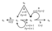
Figure 1: Alternating Data Automaton Example

Example

Figure 1 depicts an ADA with input alphabet $\Sigma=\left\{a,b\right\}$, variables $\mathbf{x}=\left\{x,y\right\}$, states $Q=\left\{q_{0},q_{1},q_{2},q_{3},q_{4}\right\}$, initial configuration $q_{0}$, final states $F=\left\{q_{3},q_{4}\right\}$ and transitions:

$$\begin{array}[]{rcl}\Delta(q_{0},a)&\equiv&q_{1}\wedge q_{2}\wedge x\approx 0\wedge y\approx 0\\ \Delta(q_{1},a)&\equiv&q_{1}\wedge q_{3}\wedge x\approx\overline{y}+1\wedge y\approx\overline{x}+1\\ \Delta(q_{1},b)&\equiv&q_{3}\wedge\overline{x}\geq\overline{y}\\ \Delta(q_{2},a)&\equiv&q_{2}\wedge x>\overline{x}\wedge y>\overline{y}\\ \Delta(q_{2},b)&\equiv&q_{4}\wedge\overline{x}>\overline{y}\end{array}$$

The missing rules, such as $\Delta(q_{0},b)$, are assumed to be $\bot$. Rules $\Delta(q_{0},a)$ and $\Delta(q_{1},a)$ are universal and there are no existential nondeterministic rules. Rules $\Delta(q_{1},a)$ and $\Delta(q_{2},a)$ compare past ($\overline{x},\overline{y}$) with present ($x,y$) values, $\Delta(q_{0},a)$ constrains the present and $\Delta(q_{1},b)$, $\Delta(q_{2},b)$ the past values, respectively. ∎

Formally, let $\mathbf{x}_{k}=\left\{x_{k}\mid x\in\mathbf{x}\right\}$, for any $k\geq 0$, be a set of time-stamped variables. For an input event $a\in\Sigma$ and a formula $\phi$, we write $\Delta(\phi,a)$ (respectively $\Delta^{k}(\phi,a)$) for the formula obtained from $\phi$ by simultaneously replacing each state $q\in\mathrm{FV}^{\mathsf{Bool}}(\phi)$ by the formula $\Delta(q,a)$ (respectively $\Delta(q,a)[\mathbf{x}_{k}/\overline{\mathbf{x}},\mathbf{x}_{k+1}/\mathbf{x}]$, for $k\geq 0$). Given a word $w=(a_{1},\nu_{1})(a_{2},\nu_{2})\ldots(a_{n},\nu_{n})$, the run of $\mathcal{A}$ over $w$ is the sequence of formulae:

$$\phi_{0}(Q)\Rightarrow\phi_{1}(Q,\mathbf{x}_{0}\cup\mathbf{x}_{1})\Rightarrow\ldots\Rightarrow\phi_{n}(Q,\mathbf{x}_{0}\cup\ldots\cup\mathbf{x}_{n})$$

where $\phi_{0}\equiv\iota$ and, for all $k\in[1,n]$, we have $\phi_{k}\equiv\Delta^{k}(\phi_{k-1},a_{k})$. Next, we slightly abuse notation and write $\Delta(\iota,a_{1},\ldots,a_{n})$ for the formula $\phi_{n}(\mathbf{x}_{0},\ldots,\mathbf{x}_{n})$ above. We say that $\mathcal{A}$ accepts $w$ iff $\mathcal{I},\nu\models\Delta(\iota,a_{1},\ldots,a_{n})$, for some valuation $\nu$ that maps: (1) each $x\in\mathbf{x}_{k}$ to $\nu_{k}(x)$, for all $k\in[1,n]$, (2) each $q\in\mathrm{FV}^{\mathsf{Bool}}(\phi_{n})\cap F$ to $\top$ and (3) each $q\in\mathrm{FV}^{\mathsf{Bool}}(\phi_{n})\setminus F$ to $\bot$. The language of $\mathcal{A}$ is the set $L(\mathcal{A})$ of words from $\Sigma[\mathbf{x}]^{*}$ accepted by $\mathcal{A}$.

Example

The following sequence is a non-accepting run of the ADA from Figure 1 on the word $(a,\left\langle 0,0\right\rangle),(a,\left\langle 1,1\right\rangle),(b,\left\langle 2,1\right\rangle)$, where $\mathsf{Data}^{\mathcal{I}}={\bf\mathbb{Z}}$ and the function symbols have standard arithmetic interpretation:

$$\begin{array}[]{l}q_{0}\stackrel{{\scriptstyle(a,\left\langle 0,0\right\rangle)}}{{\Longrightarrow}}q_{1}\wedge q_{2}\wedge x_{1}\approx 0\wedge y_{1}\approx 0\stackrel{{\scriptstyle(a,\left\langle 1,1\right\rangle)}}{{\Longrightarrow}}\\ \underbrace{q_{1}\wedge q_{2}\wedge x_{2}\approx y_{1}+1\wedge y_{2}\approx x_{1}+1}_{q_{1}}~{}\wedge~{}\underbrace{q_{2}\wedge x_{2}>x_{1}\wedge y_{2}>y_{1}}_{q_{2}}\\ \wedge~{}x_{1}\approx 0\wedge y_{1}\approx 0\stackrel{{\scriptstyle(b,\left\langle 2,1\right\rangle)}}{{\Longrightarrow}}\underbrace{q_{3}\wedge x_{2}\geq y_{2}}_{q_{1}}\wedge\underbrace{q_{4}\wedge x_{2}>y_{2}}_{q_{2}}\wedge x_{2}\approx y_{1}+1\\ \wedge~{}y_{2}\approx x_{1}+1\wedge\underbrace{q_{4}\wedge x_{2}>y_{2}}_{q_{2}}\wedge x_{2}>x_{1}\wedge y_{2}>y_{1}\wedge x_{1}\approx 0\wedge y_{1}\approx 0~{}\hfill\text{\qed}\end{array}$$

In this paper we tackle the following problems:

1. boolean closure: given automata $\mathcal{A}_{1}$ and $\mathcal{A}_{2}$, both with the same set of variables $\mathbf{x}$, do there exist automata $\mathcal{A}_{\cup}$, $\mathcal{A}_{\cap}$ and $\overline{\mathcal{A}_{1}}$ such that $L(\mathcal{A}_{\cup})=\mathcal{A}_{1}\cup\mathcal{A}_{2}$, $L(A_{\cap})=\mathcal{A}_{1}\cap\mathcal{A}_{2}$ and $L(\overline{\mathcal{A}_{1}})=\Sigma[\mathbf{x}]^{*}\setminus L(\mathcal{A}_{1})$ ?

2. emptiness: given an automaton $\mathcal{A}$, is $L(\mathcal{A})=\emptyset$ ?

It is well known that other problems, such as universality (given automaton $\mathcal{A}$ with variables $\mathbf{x}$, does $L(\mathcal{A})=\Sigma[\mathbf{x}]^{*}$?) and inclusion (given automata $\mathcal{A}_{1}$ and $\mathcal{A}_{2}$ with the same set of variables, does $L(\mathcal{A}_{1})\subseteq L(\mathcal{A}_{2})$?) can be reduced to the above problems. Observe furthermore that we do not consider cases in which the sets of variables in the two automata differ. An interesting problem in this case would be: given automata $\mathcal{A}_{1}$ and $\mathcal{A}_{2}$, with variables $\mathbf{x}_{1}$ and $\mathbf{x}_{2}$, respectively, such that $\mathbf{x}_{1}\subseteq\mathbf{x}_{2}$, does $L(\mathcal{A}_{1})\subseteq{L(\mathcal{A}_{2})}\!\!\downarrow_{{\mathbf{x}_{1}}}$, where ${L(\mathcal{A}_{2})}\!\!\downarrow_{{\mathbf{x}_{1}}}$ is the projection of the set of words $L(\mathcal{A}_{2})$ onto the variables $\mathbf{x}_{1}$? This problem is considered as future work.

III-A Boolean Closure

Given a set $Q$ of boolean variables and a set $\mathbf{x}$ of variables of sort $\mathsf{Data}$, for a formula $\phi\in\mathsf{Form}^{+}(Q,\mathbf{x})$, with no negated occurrences of the boolean variables, we define the formula $\overline{\phi}\in\mathsf{Form}^{+}(Q,\mathbf{x})$ recursively on the structure of $\phi$:

$$\begin{array}[]{lclclcl}\overline{\phi_{1}\vee\phi_{2}}&\equiv&\overline{\phi_{1}}\wedge\overline{\phi_{2}}&&\overline{\phi_{1}\wedge\phi_{2}}&\equiv&\overline{\phi_{1}}\vee\overline{\phi_{2}}\\ \overline{\neg\phi}&\equiv&\neg\overline{\phi}\text{ if $\phi$ not atom}&&\overline{\phi}&\equiv&\phi\text{ if $\phi\in Q$}\\ \overline{\phi}&\equiv&\neg\phi\text{ if $\phi\not\in Q$ atom}\end{array}$$

We have ${|{\overline{\phi}}|}={|{\phi}|}$, for every formula $\phi\in\mathsf{Form}^{+}(Q,\mathbf{x})$.

In the following let $\mathcal{A}_{i}=\left\langle\mathbf{x},Q_{i},\iota_{i},F_{i},\Delta_{i}\right\rangle$, for $i=1,2$, where w.l.o.g. we assume that $Q_{1}\cap Q_{2}=\emptyset$. We define:

$$\begin{array}[]{rcl}\mathcal{A}_{\cup}&=&\left\langle\mathbf{x},Q_{1}\cup Q_{2},\iota_{1}\vee\iota_{2},F_{1}\cup F_{2},\Delta_{1}\cup\Delta_{2}\right\rangle\\ \mathcal{A}_{\cap}&=&\left\langle\mathbf{x},Q_{1}\cup Q_{2},\iota_{1}\wedge\iota_{2},F_{1}\cup F_{2},\Delta_{1}\cup\Delta_{2}\right\rangle\\ \overline{\mathcal{A}_{1}}&=&\langle\mathbf{x},Q_{1},\overline{\iota_{1}},Q_{1}\setminus F_{1},\overline{\Delta_{1}}\rangle\end{array}$$

where $\overline{\Delta_{1}}(q,a)\equiv\overline{\Delta_{1}(q,a)}$, for all $q\in Q_{1}$ and $a\in\Sigma$. The following lemma shows the correctness of the above definitions:

Lemma 1

Given automata $\mathcal{A}_{i}=\left\langle\mathbf{x},Q_{i},\iota_{i},F_{i},\Delta_{i}\right\rangle$, for $i=1,2$, such that $Q_{1}\cap Q_{2}=\emptyset$, we have $L(\mathcal{A}_{\cup})=L(\mathcal{A}_{1})\cup L(\mathcal{A}_{2})$, $L(\mathcal{A}_{\cap})=L(\mathcal{A}_{1})\cap L(\mathcal{A}_{2})$ and $L(\overline{\mathcal{A}_{1}})=\Sigma[\mathbf{x}]^{*}\setminus L(\mathcal{A}_{1})$.

It is easy to see that ${|{\mathcal{A}_{\cup}}|}={|{\mathcal{A}_{\cap}}|}={|{\mathcal{A}_{1}}|}+{|{\mathcal{A}_{2}}|}$ and ${|{\overline{\mathcal{A}}}|}={|{\mathcal{A}}|}$, thus the automata for the boolean operations, including complementation, can be built in linear time. This matches the linear-time bounds for intersection and complementation of alternating automata over finite alphabets [3].

IV Antichains and Interpolants for Emptiness

Unlike the boolean closure properties, showed to be effectively decidable (Lemma 1), the emptiness problem is undecidable, even in very simple cases. For instance, if $\mathsf{Data}^{\mathcal{I}}$ is the set of positive integers, an ADA can simulate an Alternating Vector Addition System with States (AVASS) using only atoms $x\geq k$ and $x=\overline{x}+k$, for $k\in{\bf\mathbb{Z}}$, with the classical interpretation of the function symbols on integers. Since reachability of a control state is undecidable for AVASS [14], the emptiness problem is undecidable for ADA.

Consequently, we give up on the guarantee for termination and build semi-algorithms that meet the requirements below:

1. given an automaton $\mathcal{A}$, if $L(\mathcal{A})\neq\emptyset$, the procedure will terminate and return a word $w\in L(\mathcal{A})$, and

2. if the procedure terminates without returning such a word, then $L(\mathcal{A})=\emptyset$.

Let us fix an automaton $\mathcal{A}=\left\langle\mathbf{x},Q,\iota,F,\Delta\right\rangle$ whose (finite) input event alphabet is $\Sigma$, for the rest of this section. Given a formula $\phi\in\mathsf{Form}^{+}(Q,\mathbf{x})$ and an input event $a\in\Sigma$, we define the post-image function $\mathsf{Post}_{\mathcal{A}}(\phi,a)\equiv\exists\overline{\mathbf{x}}~{}.~{}\Delta(\phi[\overline{\mathbf{x}}/\mathbf{x}],a)\in\mathsf{Form}^{+}(Q,\mathbf{x})$, mapping each formula in $\mathsf{Form}^{+}(Q,\mathbf{x})$ to a formula defining the effect of reading the event $a$.

We generalize the post-image function to finite sequences of input events, as follows:

$$\begin{array}[]{l}\mathsf{Post}_{\mathcal{A}}(\phi,\varepsilon)\equiv\phi\hskip 14.22636pt\mathsf{Post}_{\mathcal{A}}(\phi,ua)\equiv\mathsf{Post}_{\mathcal{A}}(\mathsf{Post}_{\mathcal{A}}(\phi,u),a)\\ \mathsf{Acc}_{\mathcal{A}}(u)\equiv\mathsf{Post}_{\mathcal{A}}(\iota,u)\wedge\bigwedge_{q\in Q\setminus F}(q\rightarrow\bot)\text{, for any $u\in\Sigma^{*}$}\end{array}$$

Then the emptiness problem for $\mathcal{A}$ becomes: does there exist $u\in\Sigma^{*}$ such that the formula $\mathsf{Acc}_{\mathcal{A}}(u)$ is satisfiable? Observe that, since we ask a satisfiability query, the final states of $\mathcal{A}$ need not be constrained. A naïve semi-algorithm enumerates all finite sequences and checks the satisfiability of $\mathsf{Acc}_{\mathcal{A}}(u)$ for each $u\in\Sigma^{*}$, using a decision procedure for the theory $\mathbb{T}(\mathsf{S},\mathcal{I})$.

Since no boolean variable from $Q$ occurs under negation in $\phi$, it is easy to prove the following monotonicity property: given two formulae $\phi,\psi\in\mathsf{Form}^{+}(Q,\mathbf{x})$ if $\phi\models\psi$ then $\mathsf{Post}_{\mathcal{A}}(\phi,u)\models\mathsf{Post}_{\mathcal{A}}(\psi,u)$, for any $u\in\Sigma^{*}$. This suggest an improvement of the above semi-algorithm, that enumerates and stores only a set $U\subseteq\Sigma^{*}$ for which $\left\{\mathsf{Post}_{\mathcal{A}}(\phi,u)\mid u\in U\right\}$ forms an antichain w.r.t. the entailment partial order. This is because, for any $u,v\in\Sigma^{*}$, if $\mathsf{Post}_{\mathcal{A}}(\iota,u)\models\mathsf{Post}_{\mathcal{A}}(\iota,v)$ and $\mathsf{Acc}_{\mathcal{A}}(uw)$ is satisfiable for some $w\in\Sigma^{*}$, then $\mathsf{Post}_{\mathcal{A}}(\iota,uw)\models\mathsf{Post}_{\mathcal{A}}(\iota,vw)$, thus $\mathsf{Acc}_{\mathcal{A}}(vw)$ is satisfiable as well, and there is no need for $u$, since the non-emptiness of $\mathcal{A}$ can be proved using $v$ alone. However, even with this optimization, the enumeration of sequences from $\Sigma^{*}$ diverges in many real cases, because infinite antichains exist in many interpretations, e.g. $q\wedge x\approx 0,~{}q\wedge x\approx 1,\ldots$ for $\mathsf{Data}^{\mathcal{I}}={\bf\mathbb{N}}$.

A safety invariant for $\mathcal{A}$ is a function $\mathsf{I}:(Q\mapsto\mathbb{B})\rightarrow 2^{\mathbf{x}\mapsto\mathsf{Data}^{\mathcal{I}}}$ such that, for every boolean valuation $\beta:Q\rightarrow\mathbb{B}$, every valuation $\nu:\mathbf{x}\mapsto\mathsf{Data}^{\mathcal{I}}$ of the data variables and every finite sequence $u\in\Sigma^{*}$ of input events, the following hold:

1. $\mathcal{I},\beta\cup\nu\models\mathsf{Post}_{\mathcal{A}}(\iota,u)\Rightarrow\nu\in\mathsf{I}(\beta)$, and

2. $\nu\in\mathsf{I}(\beta)\Rightarrow\mathcal{I},\beta\cup\nu\not\models\mathsf{Acc}_{\mathcal{A}}(u)$.

If $\mathsf{I}$ satisfies only the first point above, we call it an invariant. Intuitively, a safety invariant maps every boolean valuation into a set of data valuations, that contains the initial configuration $\iota\equiv\mathsf{Post}_{\mathcal{A}}(\iota,\varepsilon)$, whose data variables are unconstrained, over-approximates the set of reachable valuations (point 1) and excludes the valuations satisfying the acceptance condition (point 2). A formula $\phi(Q,\mathbf{x})$ is said to define $\mathsf{I}$ iff for all $\beta:Q\rightarrow\mathbb{B}$ and $\nu:\mathbf{x}\rightarrow\mathsf{Data}^{\mathcal{I}}$, we have $\mathcal{I},\beta\cup\nu\models\phi$ iff $\nu\in\mathsf{I}(\beta)$.

Lemma 2

For any automaton $\mathcal{A}$, we have $L(\mathcal{A})=\emptyset$ if and only if $\mathcal{A}$ has a safety invariant.

Turning back to the issue of divergence of language emptiness semi-algorithms in the case $L(\mathcal{A})=\emptyset$, we can observe that an enumeration of input sequences $u_{1},u_{2},\ldots\in\Sigma^{*}$ can stop at step $k$ as soon as $\bigvee_{i=1}^{k}\mathsf{Post}_{\mathcal{A}}(\iota,u_{i})$ defines a safety invariant for $\mathcal{A}$. Although this condition can be effectively checked using a decision procedure for the theory $\mathbb{T}(\mathsf{S},\mathcal{I})$, there is no guarantee that this check will ever succeed.

The solution we adopt in the sequel is abstraction to ensure the termination of invariant computations. However, it is worth pointing out from the start that abstraction alone will only allow us to build invariants that are not necessarily safety invariants. To meet the latter condition, we resort to counterexample guided abstraction refinement (CEGAR).

Formally, we fix a set of formulae $\mathsf{\Pi}\subseteq\mathsf{Form}(Q,\mathbf{x})$, such that $\bot\in\mathsf{\Pi}$ and refer to these formulae as predicates. Given a formula $\phi$, we denote by ${\phi}^{\sharp}\equiv\bigwedge\left\{\pi\in\mathsf{\Pi}\mid\phi\models\pi\right\}$ the abstraction of $\phi$ w.r.t. the predicates in $\mathsf{\Pi}$. The abstract versions of the post-image and acceptance condition are defined as follows:

$$\begin{array}[]{l}{\mathsf{Post}}^{\sharp}_{\mathcal{A}}(\phi,\varepsilon)\equiv\phi\hskip 14.22636pt{\mathsf{Post}}^{\sharp}_{\mathcal{A}}(\phi,ua)\equiv{(\mathsf{Post}_{\mathcal{A}}({\mathsf{Post}}^{\sharp}_{\mathcal{A}}(\phi,u),a))}^{\sharp}\\ {\mathsf{Acc}}^{\sharp}_{\mathcal{A}}(u)\equiv{\mathsf{Post}}^{\sharp}_{\mathcal{A}}(\iota,u)\wedge\bigwedge_{q\in Q\setminus F}(q\rightarrow\bot)\text{, for any $u\in\Sigma^{*}$}\end{array}$$

Lemma 3

For any bijection $\mu:{\bf\mathbb{N}}\rightarrow\Sigma^{*}$, there exists $k>0$ such that $\bigvee_{i=0}^{k}{\mathsf{Post}}^{\sharp}_{\mathcal{A}}(\iota,\mu(i))$ defines an invariant ${\mathsf{I}}^{\sharp}$ for $\mathcal{A}$.

We are left with fulfilling point (2) from the definition of a safety invariant. To this end, suppose that, for a given set $\mathsf{\Pi}$ of predicates, the invariant ${\mathsf{I}}^{\sharp}$, defined by the previous lemma, meets point (1) but not point (2), where $\mathsf{Post}_{\mathcal{A}}$ and $\mathsf{Acc}_{\mathcal{A}}$ replace ${\mathsf{Post}}^{\sharp}_{\mathcal{A}}$ and ${\mathsf{Acc}}^{\sharp}_{\mathcal{A}}$, respectively. In other words, there exists a finite sequence $u\in\Sigma^{*}$ such that $\nu\in{\mathsf{I}}^{\sharp}(\beta)$ and $\mathcal{I},\beta\cup\nu\models{\mathsf{Acc}}^{\sharp}_{\mathcal{A}}(u)$, for some boolean $\beta:Q\rightarrow\mathbb{B}$ and data $\nu:\mathbf{x}\rightarrow\mathsf{Data}^{\mathcal{I}}$ valuations. Such a $u\in\Sigma^{*}$ is called a counterexample.

Once a counterexample $u$ is discovered, there are two possibilities. Either (i) $\mathsf{Acc}_{\mathcal{A}}(u)$is satisfiable, in which case $u$ is feasible and $L(\mathcal{A})\neq\emptyset$, or (ii) $\mathsf{Acc}_{\mathcal{A}}(u)$is unsatisfiable, in which case $u$ is spurious. In the first case, our semi-algorithm stops and returns a witness for non-emptiness, obtained from the satisfying valuation of $\mathsf{Acc}_{\mathcal{A}}(u)$ and in the second case, we must strenghten the invariant by excluding from ${\mathsf{I}}^{\sharp}$ all pairs $(\beta,\nu)$ such that $\mathcal{I},\beta\cup\nu\models{\mathsf{Acc}}^{\sharp}_{\mathcal{A}}(u)$. This strenghtening is carried out by adding to $\mathsf{\Pi}$ several predicates that are sufficient to exclude the spurious counterexample.

In general, given an unsatisfiable conjunction $\Phi\equiv\phi_{1}(X_{0},X_{1})\wedge\phi_{2}(X_{1},X_{2})\wedge\ldots\wedge\phi_{n}(X_{n-1},X_{n})$ of time-stamped variables $X_{i}=\left\{x_{i}\mid x\in X\right\}$ of any sort, a solution of the interpolation problem $\Phi$, simply called an interpolant, is a tuple $\left\langle I_{0}(X),I_{1}(X),\ldots,I_{n}(X)\right\rangle$ such that: (i) $I_{0}\equiv\top$, (ii) $I_{i-1}[X_{i-1}/X]\wedge\phi_{i}(X_{i-1},X_{i})\models I_{i}[X_{i}/X]$, for all $i\in[1,n]$, and (iii) $I_{n}\equiv\bot$. In the following, we shall assume the existence of an interpolating decision procedure for $\mathbb{T}(\mathsf{S},\mathcal{I})$.

A classical method for abstraction refinement is to add the elements of the interpolant obtained from a proof of spuriousness to the set of predicates. This guarantees progress, meaning that the particular spurious counterexample, from which the interpolant was generated, will never be revisited in the future. Though not always, in many practical test cases this progress property eventually yields a safety invariant.

Given a non-empty spurious counterexample $u=a_{1}\ldots a_{n}$, where $n>0$, we consider the following interpolation problem:

$$\Theta(u) \equiv \theta_{0}(Q_{0})\wedge\theta_{1}(Q_{0}\cup Q_{1},\mathbf{x}_{0}\cup\mathbf{x}_{1})\wedge\ldots$$

$$\wedge~{}\theta_{n}(Q_{n-1}\cup Q_{n},\mathbf{x}_{n-1}\cup\mathbf{x}_{n})\wedge\theta_{n+1}(Q_{n})$$

where $Q_{k}=\left\{q_{k}\mid q\in Q\right\}$, $k\in[0,n]$ are time-stamped sets of boolean variables corresponding to the set $Q$ of states of $\mathcal{A}$. The first conjunct $\theta_{0}(Q_{0})\equiv\iota[Q_{0}/Q]$ is the initial configuration of $\mathcal{A}$, with every $q\in\mathrm{FV}^{\mathsf{Bool}}(\iota)$ replaced by $q_{0}$. The definition of $\theta_{k}$, for all $k\in[1,n]$, uses replacement sets $R_{\ell}\subseteq Q_{\ell}$, $\ell\in[0,n]$, which are defined inductively below:

• $R_{0}=\mathrm{FV}^{\mathsf{Bool}}(\theta_{0})$,

• $\theta_{\ell}\equiv\bigwedge_{q_{\ell-1}\in R_{\ell-1}}(q_{\ell-1}\rightarrow\Delta(q,a_{\ell})[Q_{\ell}/Q,\mathbf{x}_{\ell-1}/\overline{\mathbf{x}},\mathbf{x}_{\ell}/\mathbf{x}])$ and $R_{\ell}=\mathrm{FV}^{\mathsf{Bool}}(\theta_{\ell})\cap Q_{\ell}$, for each $\ell\in[1,n]$.

• $\theta_{n+1}(Q_{n})\equiv\bigwedge_{q\in Q\setminus F}(q_{n}\rightarrow\bot)$.

The intuition is that $R_{0},\ldots,R_{n}$ are the sets of states replaced, $\theta_{0},\ldots,\theta_{n}$ are the sets of transition rules fired on the run of $\mathcal{A}$ over $u$ and $\theta_{n+1}$ is the acceptance condition, which forces the last remaining non-final states to be false.

Moreover, we require that an interpolant $\left\langle\top,I_{0},\ldots,I_{n},\bot\right\rangle$ for the interpolation problem $\Theta(u)$ does not have negative occurrences of states, i.e. $I_{i}\in\mathsf{Form}^{+}(Q,\mathbf{x})$, for all $i\in[0,n]$. Such an interpolant can always be built, as showed below:

Proposition 1

If $\Theta(a_{1}\ldots a_{n})$ is unsatisfiable then one can build an interpolant $\left\langle\top,I_{0},\ldots,I_{n},\bot\right\rangle$ for $\Theta(a_{1}\ldots a_{n})$, such that $I_{i}\in\mathsf{Form}^{+}(Q,\mathbf{x})$, for all $i\in[0,n]$.

We recall that a run of $\mathcal{A}$ over $u$ is a sequence:

$$\phi_{0}(Q)\Rightarrow\phi_{1}(Q,\mathbf{x}_{0}\cup\mathbf{x}_{1})\Rightarrow\ldots\Rightarrow\phi_{n}(Q,\mathbf{x}_{0}\cup\ldots\cup\mathbf{x}_{n})$$

where $\phi_{0}$ is the initial configuration $\iota$ and for each $k>0$, $\phi_{k}$ is obtained from $\phi_{k-1}$ by replacing each state $q\in\mathrm{FV}^{\mathsf{Bool}}(\phi_{k-1})$ by the formula $\Delta(q,a_{k})[\mathbf{x}_{k-1}/\overline{\mathbf{x}},\mathbf{x}_{k}/\mathbf{x}]$, given by the transition function of $\mathcal{A}$. Observe that, because the states are replaced with transition formulae when moving one step in a run, these formulae lose track of the control history and are not suitable for producing interpolants that relate states and data.

The main idea behind the above definition of the interpolation problem is that we would like to obtain an interpolant $\left\langle\top,I_{0}(Q),I_{1}(Q,\mathbf{x}),\ldots,I_{n}(Q,\mathbf{x}),\bot\right\rangle$ whose formulae combine states with the data constraints that must hold locally, whenever the control reaches a certain boolean configuration. This association of states with data valuations is tantamount to defining efficient semi-algorithms, based on lazy abstraction [8]. Furthermore, the abstraction defined by the interpolants generated in this way can also over-approximate the control structure of an automaton, in addition to the sets of data values encountered throughout its runs.

The correctness of this interpolation-based abstraction refinement setup is captured by the progress property below, which guarantees that adding the formulae of an interpolant for $\Theta(u)$ to the set $\mathsf{\Pi}$ of predicates suffices to exclude the spurious counterexample $u$ from future searches.

Lemma 4

For any sequence $u=a_{1}\ldots a_{n}\in\Sigma^{*}$, if $\mathsf{Acc}_{\mathcal{A}}(u)$ is unsatisfiable, the following hold:

1. $\Theta(u)$ is unsatisfiable, and

2. if $\left\langle\top,I_{0},\dots,I_{n},\bot\right\rangle$ is an interpolant for $\Theta(u)$ such that $\left\{I_{i}\mid i\in[0,n]\right\}\subseteq\mathsf{\Pi}$ then ${\mathsf{Acc}}^{\sharp}_{\mathcal{A}}(u)$ is unsatisfiable.

V Lazy Predicate Abstraction for ADA Emptiness

We have now all the ingredients to describe the first emptiness checking semi-algorithm for alternating data automata. Algorithm 1 builds an abstract reachability tree (ART) whose nodes are labeled with formulae over-approximating the concrete sets of configurations, and a covering relation between nodes in order to ensure that the set of formulae labeling the nodes in the ART forms an antichain. Any spurious counterexample is eliminated by computing an interpolant and adding its formulae to the set of predicates (cf. Lemma 4).

input: an ADA $\mathcal{A}=\left\langle\mathbf{x},Q,\iota,F,\Delta\right\rangle$ over the alphabet $\Sigma$ of input events

output: $\mathtt{true}$ if $L(\mathcal{A})=\emptyset$ and a data word $w\in L(\mathcal{A})$ otherwise

1:let $\mathcal{T}=\left\langle N,E,\mathtt{r},\Lambda,\lhd\right\rangle$ be an ART

2:initially $N=E=\lhd=\emptyset$, $\Lambda=\left\{(\mathtt{r},\iota)\right\}$, $\mathsf{\Pi}=\left\{\bot\right\}$, $\mathtt{WorkList}=\left\langle\mathtt{r}\right\rangle$,

3:while $\mathtt{WorkList}\neq\emptyset$ do

4:    dequeue $n$ from $\mathtt{WorkList}$

5:    $N\leftarrow N\cup\left\{n\right\}$

6:    let $\lambda(n)=a_{1}\ldots a_{k}$ be the label of the path from $\mathtt{r}$ to $n$

7:    if ${\mathsf{Post}}^{\sharp}_{\mathcal{A}}(\lambda(n))$ is satisfiable then $\triangleright$ counterexample candidate

8:       if $\mathsf{Acc}_{\mathcal{A}}(u)$ is satisfiable then $\triangleright$ feasible counterexample

9:          get model $(\beta,\nu_{1},\ldots,\nu_{k})$ of $\mathsf{Acc}_{\mathcal{A}}(\lambda(n))$

10:          return $w=(a_{1},\nu_{1})\ldots(a_{k},\nu_{k})$ $\triangleright$ $w\in L(\mathcal{A})$ by construction

11:       else$\triangleright$ spurious counterexample

12:          $p\leftarrow\textsc{FindPivot}(\lambda(n),\mathcal{T})$

13:          $v\leftarrow\textsc{LeastInfeasibleSuffix}(\lambda(n),\mathcal{T})$

14:          $\mathsf{\Pi}\leftarrow\mathsf{\Pi}\cup\left\{I_{0},\ldots,I_{\ell}\right\}$, where $\left\langle\top,I_{0},\ldots,I_{\ell},\bot\right\rangle$ is an interpolant for $\Psi(v)$

15:          let $\mathcal{S}=\left\langle N^{\prime},E^{\prime},p,\Lambda^{\prime},\lhd^{\prime}\right\rangle$ be the subtree of $\mathcal{T}$ rooted at $p$

16:          for $(m,q)\in\lhd$ such that $q\in N^{\prime}$ do

17:             remove $m$ from $N$ and enqueue $m$ into $\mathtt{WorkList}$

18:             remove $\mathcal{S}$ from $\mathcal{T}$

19:             enqueue $p$ into $\mathtt{WorkList}$ $\triangleright$ recompute the subtree rooted at $p$                  

20:    else

21:       for $a\in\Sigma$ do $\triangleright$ expand $n$

22:          $\phi\leftarrow{\mathsf{Post}}^{\sharp}_{\mathcal{A}}(\Lambda(n),a)$

23:          if exist $m\in N$ such that $\phi\models\Lambda(m)$ then

24:             $\lhd\leftarrow\lhd\cup\left\{(n,m)\right\}$ $\triangleright$ $m$ covers $n$

25:          else

26:             let $s$ be a fresh node

27:             $E\leftarrow E\cup\left\{(n,a,s)\right\}$

28:             $\Lambda\leftarrow\Lambda\cup\left\{(s,\phi)\right\}$

29:             $R\leftarrow\left\{m\in\mathtt{WorkList}\mid\Lambda(m)\models\phi\right\}$ $\triangleright$ worklist nodes covered by $s$

30:             for $r\in R$ do

31:                for $m\in N$ such that $(m,b,r)\in E$, $b\in\Sigma$ do

32:                   $\lhd\leftarrow\lhd\cup\left\{(m,s)\right\}$ $\triangleright$ redirect covered children from $R$ into $s$                 

33:                for $(m,r)\in\lhd$ do

34:                   $\lhd\leftarrow\lhd\cup\left\{(m,s)\right\}$ $\triangleright$ redirect covered nodes from $R$ into $s$                              

35:             remove $R$ from $\mathcal{T}$

36:             enqueue $s$ into $\mathtt{WorkList}$                      

37:return $\mathtt{true}$

Algorithm 1 Lazy Predicate Abstraction for ADA Emptiness

Formally, an ART is tuple $\mathcal{T}=\left\langle N,E,\mathtt{r},\Lambda,R,T,\lhd\right\rangle$, where:

• $N$ is a set of nodes,

• $E\subseteq N\times\Sigma\times N$ is a set of edges,

• $\mathtt{r}\in N$ is the root of the directed tree $(N,E)$,

• $\Lambda:N\rightarrow\mathsf{Form}(Q,\mathbf{x})$ is a labeling of the nodes with formulae, such that $\Lambda(\mathtt{r})=\iota$,

• $R:N\rightarrow 2^{Q}$ is a labeling of nodes with replacement sets, such that $R(\mathtt{r})=\mathrm{FV}^{\mathsf{Bool}}(\iota)$,

• $T:E\rightarrow\bigcup_{i=0}^{\infty}\mathsf{Form}^{+}(Q_{i},\mathbf{x}_{i},Q_{i+1},\mathbf{x}_{i+1})$ is a labeling of edges with time-stamped formulae, and

• $\lhd\subseteq N\times N$ is a set of covering edges.

Each node $n\in N$ corresponds to a unique path from the root to $n$, labeled by a sequence $\lambda(n)\in\Sigma^{*}$ of input events. The least infeasible suffix of $\lambda(n)$ is the smallest sequence $v=a_{1}\ldots a_{k}$, such that $\lambda(n)=wv$, for some $w\in\Sigma^{*}$ and the following formula is unsatisfiable:

$$\Psi(v)\equiv\Lambda(p)[Q_{0}/Q]\wedge\theta_{1}(Q_{0}\cup Q_{1},\mathbf{x}_{0}\cup\mathbf{x}_{1})\wedge\ldots\wedge\theta_{k+1}(Q_{k})$$ (2)

where $\theta_{1},\ldots,\theta_{k+1}$ are defined as in (IV) and $\theta_{0}\equiv\Lambda(p)[Q_{0}/Q]$. The pivot of $n$ is the node $p$ corresponding to the start of the least infeasible suffix. We assume the existence of two functions $\textsc{FindPivot}(u,\mathcal{T})$ and $\textsc{LeastInfeasibleSuffix}(u,\mathcal{T})$ that return the pivot and least infeasbile suffix of a sequence $u\in\Sigma^{*}$ in an ART $\mathcal{T}$, without detailing their implementation.

With these considerations, Algorithm 1 uses a worklist iteration to build an ART. We keep newly expanded nodes of $\mathcal{T}$ in a queue $\mathtt{WorkList}$, thus implementing a breadth-first exploration strategy, which guarantees that the shortest counterexamples are explored first. When the search encounters a counterexample candidate $u$, it is checked for spuriousness. If the counterexample is feasible, the procedure returns a data word $w\in L(\mathcal{A})$, which interleaves the input events of $u$ with the data valuations from the model of $\mathsf{Acc}_{\mathcal{A}}(u)$ (since $u$ is feasible, clearly $\mathsf{Acc}_{\mathcal{A}}(u)$ is satisfiable). Otherwise, if $u$ is spurious, we compute its pivot $p$ (line 12), add the interpolants for the least unfeasible suffix of $u$ to the set of predicates $\mathsf{\Pi}$, remove and recompute the subtree of $\mathcal{T}$ rooted at $p$.

Termination of Algorithm 1 depends on the ability of a given interpolating decision procedure for the combined boolean and data theory $\mathbb{T}(\mathsf{S},\mathcal{I})$ to provide interpolants that yield a safety invariant, whenever $L(\mathcal{A})=\emptyset$. In this case, we use the covering relation $\lhd$ to ensure that, when a newly generated node is covered by a node already in $N$, it is not added to the worklist, thus cutting the current branch of the search.

Formally, for any two nodes $n,m\in N$, we have $n\lhd m$ iff ${\mathsf{Post}}^{\sharp}_{\mathcal{A}}(\Lambda(n),a)\models\Lambda(m)$ for some $a\in\Sigma$, in other words, if $n$ has a successor whose label entails the label of $m$.

(a)	(b)
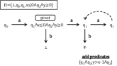
(c)	(d)

Figure 2: Proving Emptiness of the Automaton from Fig. 1 by Algorithm 1

Example

Consider the automaton given in Figure 1. First, Algorithm 1 fires the sequence $a$, and since there are no other formulae than $\bot$ in $\mathsf{\Pi}$, the successor of $\iota\equiv q_{0}$ is $\top$, in Figure 2 (a). The spuriousness check for $a$ yields the root of the ART as pivot and the interpolant $\left\langle q_{0},q_{1}\right\rangle$, which is added to the set $\mathsf{\Pi}$. Then the $\top$ node is removed and the next time $a$ is fired, it creates a node labeled $q_{1}$. The second sequence $aa$ creates a successor node $q_{1}$, which is covered by the first, depicted with a dashed arrow, in Figure 2 (b). The third sequence is $ab$, which results in a new uncovered node $\top$ and triggers a spuriousness check. The new predicate obtained from this check is $x\leq 0\wedge q_{2}\wedge y\geq 0$ and the pivot is again the root. Then the entire ART is rebuilt with the new predicates and the fourth sequence $aab$ yields an uncovered node $\top$, in Figure 2 (c). The new pivot is the endpoint of $a$ and the newly added predicates are $q_{1}\wedge q_{2}$ and $y>x-1\wedge q_{2}$. Finally, the ART is rebuilt from the pivot node and finally all nodes are covered, thus proving the emptiness of the automaton, in Figure 2 (d). ∎

The correctness of Algorithm 1 is proved below:

Theorem 1

Given an automaton $\mathcal{A}$, such that $L(\mathcal{A})\neq\emptyset$, Algorithm 1 terminates and returns a word $w\in L(\mathcal{A})$. If Algorithm 1 terminates reporting $\mathtt{true}$, then $L(\mathcal{A})=\emptyset$.

VI Checking ADA Emptiness with Impact

As pointed out by a number of authors, the bottleneck of predicate abstraction is the high cost of reconstructing parts of the ART, subsequent to the refinement of the set of predicates. The main idea of the Impact  procedure [15] is that this can be avoided and the refinement (strenghtening of the node labels of the ART) can be performed in-place. This refinement step requires an update of the covering relation, because a node that used to cover another node might not cover it after the strenghtening of its label.

We consider a total alphabetical order $\prec$ on $\Sigma$ and lift it to the total lexicographical order $\prec^{*}$ on $\Sigma^{*}$. A node $n\in N$ is covered if $(n,p)\in\lhd$ or it has an ancestor $m$ such that $(m,p)\in\lhd$, for some $p\in N$. A node $n$ is closed if it is covered, or $\Lambda(n)\not\models\Lambda(m)$ for all $m\in N$ such that $\lambda(m)\prec^{*}\lambda(n)$. Observe that we use the coverage relation $\lhd$ here with a different meaning than in Algorithm 1.

input: an ADA $\mathcal{A}=\left\langle\mathbf{x},Q,\iota,F,\Delta\right\rangle$ over the alphabet $\Sigma$ of input events

output: $\mathtt{true}$ if $L(\mathcal{A})=\emptyset$ and a data word $w\in L(\mathcal{A})$ otherwise

1:let $\mathcal{T}=\left\langle N,E,\mathtt{r},\Lambda,R,T,\lhd\right\rangle$ be an ART

2:initially $N=E=T=\lhd=\emptyset$, $\Lambda=\left\{(\mathtt{r},\iota)\right\}$, $R=\mathrm{FV}^{\mathsf{Bool}}(\iota[Q_{0}/Q])$, $\mathtt{WorkList}=\left\{\mathtt{r}\right\}$

3:while $\mathtt{WorkList}\neq\emptyset$ do

4:    dequeue $n$ from $\mathtt{WorkList}$

5:    $N\leftarrow N\cup\left\{n\right\}$

6:    let $(\mathtt{r},a_{1},n_{1}),(n_{1},a_{2},n_{2}),\ldots,(n_{k-1},a_{k},n)$ be the path from $\mathtt{r}$ to $n$

7:    if $\mathsf{Acc}_{\mathcal{A}}(a_{1}\ldots a_{k})$ is satisfiable then $\triangleright$ counterexample is feasible

8:       get model $(\beta,\nu_{1},\ldots,\nu_{k})$ of $\mathsf{Acc}_{\mathcal{A}}(\lambda(n))$

9:       return $w=(a_{1},\nu_{1})\ldots(a_{k},\nu_{k})$ $\triangleright$ $w\in L(\mathcal{A})$ by construction

10:    else$\triangleright$ spurious counterexample

11:       let $\left\langle\top,I_{0},\ldots,I_{k},\bot\right\rangle$ be an interpolant for $\Theta(a_{1}\ldots a_{k})$

12:       $b\leftarrow\mathtt{false}$

13:       for $i=0,\ldots,k$ do

14:          if $\Lambda(n_{i})\not\models I_{i}$ then

15:             $\lhd\leftarrow\lhd\setminus\left\{(m,n_{i})\in\lhd\mid m\in N\right\}$

16:             $\Lambda(n_{i})\leftarrow\Lambda(n_{i})\wedge I_{i}$ $\triangleright$ strenghten the label of $n_{i}$

17:             if $\neg b$ then

18:                $b\leftarrow\textsc{Close}(n_{i})$                                   

19:    if $n$ is not covered then

20:       for $a\in\Sigma$ do $\triangleright$ expand $n$

21:          let $s$ be a fresh node and $e=(n,a,s)$ be a new edge

22:          $E\leftarrow E\cup\left\{e\right\}$

23:          $\Lambda\leftarrow\Lambda\cup\left\{(s,\top)\right\}$

24:          $T\leftarrow T\cup\left\{(e,\theta_{k})\right\}$

25:          $R\leftarrow R\cup\{(s,\bigcup_{q\in R(n)}\mathrm{FV}^{\mathsf{Bool}}(\Delta(q,a)))\}$

26:          enqueue $s$ into $\mathtt{WorkList}$            

27:return $\mathtt{true}$

1:function Close($x$) returns $\mathsf{Bool}$

2:    for $y\in N$ such that $\lambda(y)\prec^{*}\lambda(x)$ do

3:       if $\Lambda(x)\models\Lambda(y)$ then

4:          $\lhd\leftarrow\left(\lhd\setminus\left\{(p,q)\in\lhd\mid\text{$q$ is $x$ or a successor of $x$}\right\}\right)\cup\left\{(x,y)\right\}$

5:          return $\mathtt{true}$            

6:    return $\mathtt{false}$

Algorithm 2 Impact  for ADA Emptiness

The execution of Algorithm 2 consists of three phases: close, refine and expand. Let $n$ be a node removed from the worklist at line 4. If $\mathsf{Acc}_{\mathcal{A}}(\lambda(n))$ is satisfiable, the counterexample $\lambda(n)$ is feasible, in which case a model of $\mathsf{Acc}_{\mathcal{A}}(\lambda(n))$ is obtained and a word $w\in L(\mathcal{A})$ is returned. Otherwise, $\lambda(n)$ is a spurious counterexample and the procedure enters the refinement phase (lines 11-18). The interpolant for $\Theta(\lambda(n))$ (cf. formula IV) is used to strenghten the labels of all the ancestors of $n$, by conjoining the formulae of the interpolant to the existing labels.

In this process, the nodes on the path between $\mathtt{r}$ and $n$, including $n$, might become eligible for coverage, therefore we attempt to close each ancestor of $n$ that is impacted by the refinement (line 18). Observe that, in this case the call to Close must uncover each node which is covered by a successor of $n$ (line 4 of the Close function). This is required because, due to the over-approximation of the sets of reachable configurations, the covering relation is not transitive, as explained in [15]. If Close adds a covering edge $(n_{i},m)$ to $\lhd$, it does not have to be called for the successors of $n_{i}$ on this path, which is handled via the boolean flag $b$.

Finally, if $n$ is still uncovered (it has not been previously covered during the refinement phase) we expand $n$ (lines 20-26) by creating a new node for each successor $s$ via the input event $a\in\Sigma$ and inserting it into the worklist.

(a)

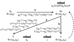
(b)

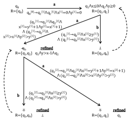
(c)

Figure 3: Proving Emptiness of the Automaton from Fig. 1 by Algorithm 2 (1/2)

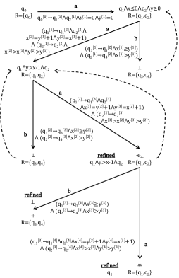
Figure 4: Proving Emptiness of the Automaton from Fig. 1 by Algorithm 2 (2/2)

Example

We show the execution of Algorithm 2 on the automaton from Figure 1. Initially, the procedure fires the sequence $a$, whose endpoint is labeled with $\top$, in Figure 3 (a). Since this node is uncovered, we check the spuriousness of the counterexample $a$ and refine the label of the node to $q_{1}$. Since the node is still uncovered, two successors, labeled with $\top$ are computed, corresponding to the sequences $aa$ and $ab$, in Figure 3 (b). The spuriousness check for $aa$ yields the interpolant $\left\langle q_{0},x\leq 0\wedge q_{2}\wedge y\geq 0\right\rangle$ which strenghtens the label of the endpoint of $a$ from $q_{1}$ to $q_{1}\wedge x\leq 0\wedge q_{2}\wedge y\geq 0$. The sequence $ab$ is also found to be spurious, which changes the label of its endpoint from $\top$ to $\bot$, and also covers it (depicted with a dashed edge). Since the endpoint of $aa$ is not covered, it is expanded to $aaa$ and $aab$, in Figure 3 (c). Both sequences $aaa$ and $aab$ are found to be spurious, and the enpoint of $aab$, whose label has changed from $\top$ to $\bot$, is now covered. In the process, the label of $aa$ has also changed from $q_{1}$ to $q_{1}\wedge y>x-1\wedge q_{2}$, due to the strenghtening with the interpolant from $aab$. Finally, the only uncovered node $aaa$ is expanded to $aaaa$ and $aaab$, both found to be spurious, in Figure 4. The refinement of $aaab$ causes the label of $aaa$ to change from $q_{1}$ to $q_{1}\wedge y>x-1\wedge q_{2}$ and this node is now covered by $aa$. Since its successors are also covered, there are no uncovered nodes and the procedure returns $\mathtt{true}$. ∎

Theorem 2

Given an automaton $\mathcal{A}$, such that $L(\mathcal{A})\neq\emptyset$, Algorithm 2 terminates and returns a word $w\in L(\mathcal{A})$. If Algorithm 2 terminates reporting $\mathtt{true}$, then $L(\mathcal{A})=\emptyset$.

VII Experimental Evaluation

We have implemented both Algorithm 1 and 2 in a prototype tool that uses the Z3 SMT solver for the satisfiability queries and interpolant generation, in the theory of linear integer arithmetic (LIA) combined with booleans. We compared both algorithms with a previous implementation of a trace inclusion procedure, called Includer, that uses on-the-fly determinisation and lazy predicate abstraction with interpolant-based refinement [11] in the LIA theory, without booleans.

The results of the experiments are given in Table I. We applied the tool first to several array logic entailments, which occur as verification conditions for imperative programs with arrays [2] (array_shift, array_simple, array_rotation 1+2) available online [17]. Next, we applied it on proving safety properties of hardware circuits (hw1+2) [20]. Finally, we considered two timed communication protocols, consisting of systems that are asynchronous compositions of timed automata, whom correctness specifications are given by timed automata monitors: a timed version of the Alternating Bit Protocol (abp) [23] and a controller of a railroad crossing (train) [9]. All results were obtained on an Intel(R) Core(TM) i7-4650U CPU @ 1.70GHz with 8GB of RAM. The automata sizes are in bytes and the execution times are in seconds.

Example	${|{\mathcal{A}}|}$	$L(\mathcal{A})=\emptyset$ ?	Algorithm 1	Algorithm 2	Includer
simple1	309	no	0.641	0.061	0.021
simple2	504	yes	0.667	0.179	0.031
simple3	214	yes	0.825	0.150	0.051
array_shift	874	yes	2.138	0.209	0.060
array_simple	3440	yes	timeout	16.435	5.496
array_rotation1	1834	yes	6.827	0.865	0.114
array_rotation2	15182	yes	timeout	timeout	23.056
abp	6909	no	8.292	1.410	1.715
train	1823	yes	16.989	2.738	0.308
hw1	322	yes	1.566	0.298	0.159
hw2	674	yes	22.914	0.552	0.419

TABLE I:

As in the non-deterministic case [15], Impact  outperforms lazy predicate abstraction for checking emptiness by at least one order of magnitude. However, both our implementations are slower than Includer, on average (except for the abp example). The reason for this is currently under investigation, one possible bottleneck being the hardness of the combined (LIA+booleans) interpolation problems, as opposed to converting the entire formula into DNF, eliminating the boolean variables and using interpolation in the pure LIA theory.

-A Proof of Lemma 1

Proposition 2

Given a formula $\phi\in\mathsf{Form}^{+}(Q,\mathbf{x})$ and a valuation $\nu$ mapping each $q\in Q$ to a value $\nu(q)\in\mathbb{B}$ and each $x\in\mathbf{x}$ to a value $\nu(x)\in\mathsf{Data}^{\mathcal{I}}$, let $\nu^{\prime}$ be the valuation that assigns each $q\in Q$ the value $\neg\nu(q)$ and each $x\in\mathbf{x}$ the value $\nu(x)$. Then we have $\mathcal{I},\nu\models\phi$ if and only if $\mathcal{I},\nu^{\prime}\not\models\overline{\phi}$.

Proof:

Immediate, by induction on the structure of $\phi$. ∎

References

- [1] R. Alur and D. L. Dill. A theory of timed automata. Theor. Comput. Sci., 126(2):183–235, 1994.
- [2] M. Bozga, P. Habermehl, R. Iosif, F. Konecný, and T. Vojnar. Automatic verification of integer array programs. In Proc. of CAV’09, volume 5643 of LNCS, pages 157–172, 2009.
- [3] A. K. Chandra, D. C. Kozen, and L. J. Stockmeyer. Alternation. J. ACM, 28(1):114–133, 1981.
- [4] L. D’Antoni, Z. Kincaid, and F. Wang. A symbolic decision procedure for symbolic alternating finite automata. CoRR, abs/1610.01722, 2016.
- [5] M. De Wulf, L. Doyen, N. Maquet, and J. F. Raskin. Antichains: Alternative algorithms for ltl satisfiability and model-checking. In TACAS 2008, Proceedings, pages 63–77. Springer, 2008.
- [6] A. Farzan, Z. Kincaid, and A. Podelski. Proof spaces for unbounded parallelism. SIGPLAN Not., 50(1):407–420, Jan. 2015.
- [7] S. Grebenshchikov, N. P. Lopes, C. Popeea, and A. Rybalchenko. Synthesizing software verifiers from proof rules. SIGPLAN Not., 47(6):405–416, June 2012.
- [8] T. A. Henzinger, R. Jhala, R. Majumdar, and G. Sutre. Lazy abstraction. SIGPLAN Not., 37(1):58–70, Jan. 2002.
- [9] T. A. Henzinger, X. Nicollin, J. Sifakis, and S. Yovine. Symbolic model checking for real-time systems. Information and Computation, 111:394–406, 1992.
- [10] K. Hoder and N. Bjørner. Generalized property directed reachability. In SAT 2012. Proceedings, pages 157–171. Springer, 2012.
- [11] R. Iosif, A. Rogalewicz, and T. Vojnar. Abstraction refinement and antichains for trace inclusion of infinite state systems. In TACAS 2016, Proceedings, pages 71–89, 2016.
- [12] M. Kaminski and N. Francez. Finite-memory automata. Theor. Comput. Sci., 134(2):329–363, Nov. 1994.
- [13] S. Lasota and I. Walukiewicz. Alternating timed automata. In FOSSACS 2005, Proceedings, pages 250–265. Springer, 2005.
- [14] P. Lincoln, J. Mitchell, A. Scedrov, and N. Shankar. Decision problems for propositional linear logic. Annals of Pure and Applied Logic, 56(1):239 – 311, 1992.
- [15] K. L. McMillan. Lazy abstraction with interpolants. In Proc. of CAV’06, volume 4144 of LNCS. Springer, 2006.
- [16] K. L. McMillan. Lazy annotation revisited. In CAV2014, Proceedings, pages 243–259. Springer International Publishing, 2014.
- [17] Numerical Transition Systems Repository. http://http://nts.imag.fr/index.php/Flata, 2012.
- [18] J. Ouaknine and J. Worrell. On the language inclusion problem for timed automata: closing a decidability gap. In Proceedings of LICS 2004., pages 54–63, 2004.
- [19] A. Pnueli. The temporal logic of programs. In Proceedings of the 18th Annual Symposium on Foundations of Computer Science, SFCS ’77, pages 46–57. IEEE, 1977.
- [20] A. Smrcka and T. Vojnar. Verifying parametrised hardware designs via counter automata. In HVC’07, pages 51–68, 2007.
- [21] M. Vardi and P. Wolper. Reasoning about infinite computations. Information and Computation, 115(1):1 – 37, 1994.
- [22] M. Veanes, P. Hooimeijer, B. Livshits, D. Molnar, and N. Bjorner. Symbolic finite state transducers: Algorithms and applications. In Proc. of POPL’12. ACM, 2012.
- [23] A. Zbrzezny and A. Polrola. Sat-based reachability checking for timed automata with discrete data. Fundamenta Informaticae, 79:1–15, 2007.