Measuring the effects of Loop Quantum Cosmology in the CMB data

Spyros Basilakos^a,2, Vahid Kamali^b,3, Ahmad Mehrabi^b,4

^aAcademy of Athens, Research Center for Astronomy and Applied Mathematics, Soranou Efesiou 4, 11527, Athens, Greece

^bDepartment of Physics, Bu-Ali Sina University, Hamedan 65178, 016016, Iran

(Submission date: March 30, 2017)

Abstract

In this Essay we investigate the observational signatures of Loop Quantum Cosmology (LQC) in the CMB data. First, we concentrate on the dynamics of LQC and we provide the basic cosmological functions. We then obtain the power spectrum of scalar and tensor perturbations in order to study the performance of LQC against the latest CMB data. We find that LQC provides a robust prediction for the main slow-roll parameters, like the scalar spectral index and the tensor-to-scalar fluctuation ratio, which are in excellent agreement within $1\sigma$ with the values recently measured by the Planck collaboration. This result indicates that LQC can be seen as an alternative scenario with respect to that of standard inflation.

Recent studies of the Cosmic Microwave Background (CMB) have opened a new window for early cosmology. Specifically, based on Planck data Ade:2015lrj ; Keck15 it has been found that the inflationary models which are in agreement with the data are those with very low tensor-to-scalar fluctuation ratio $r=\frac{P_{t}}{P_{s}}\ll 1$, with a scalar spectral index $n_{s}\simeq 0.96$ and no appreciable running. Actually, the upper bound imposed by Planck team Ade:2015lrj , on this ratio, as a result of the non-observation of B-modes, is $r<0.11$ which implies that $H\lesssim 10^{-5}M_{p}$, where $M_{p}\simeq 1.22\times 10^{19}$Gev.

After a long period of the successful inflationary paradigm, cosmology still lacks a framework in which the universe at Planck scale smoothly evolves to the CMB era. In the light of the Planck results Ade:2015lrj , a heated debate is taking place in the literature about the implementation of LQC to CMB data. Recently, Ashtekar and Gupt Gupt17 using various correlation functions for scalar perturbations found that LQC is favored by Planck, while standard (cold) inflation can not accommodate the data at large angular scales ($l\leq 30$). The intense discussion is going on and the aim of the present Essay is to contribute to this debate. Here we focus on the dynamical behavior of the effective Loop Quantum Gravity (LQG) theory via the Hubble expansion, and investigate the performance of LQC against the latest Planck data in the slow-roll regime.

Loop Quantum Cosmology: It is the framework that implements the basic cosmological principles in LQG theory Boj2005 in which canonical quantization of gravity is given in terms of the so called Ashtekar-Barbero connection variables Ashtekar:2003hd . Specifically, the phase space of classical general relativity can be spanned by conjugate variables $A_{j}^{i}$ (connection) and $E_{i}^{j}$ (triad) on a $3-manifold$ $\mathcal{M}$ which encodes curvature and spatial geometry respectively. At the level of LQC due to the homogeneous and isotropic symmetries the phase space is characterized by a single connection $c$ and a single triad $p$, while the Poisson bracket is given by $\{c,p\}=\frac{8\pi\gamma}{3M_{p}^{2}}$, where $\gamma\simeq 0.2375$ is the dimensionless Barbero-Immirzi parameter. In the context of FRW metric the above variables take the form $c=\gamma\dot{a}$ and $p=a^{2}$, where $a(t)$ is the scale factor of the universe. Based on the pair $\{c,p\}$ Ref.Singh:2005xg proposed an effective theory of LQG which is appropriate for cosmology. In particular, the effective Hamiltonian is given by $\mathcal{H}_{\rm eff}=-\frac{3\sqrt{p}}{\gamma\overline{\mu}^{2}}\sin^{2}(\overline{\mu}c)+\mathcal{H}_{m}$, where $\mathcal{H}_{m}$ is the matter Hamiltonian and $\overline{\mu}$ is associated to the minimal area of LQG. Using the effective Hamilton equation $\dot{p}=\{p,\mathcal{H}_{\rm eff}\}=-\frac{\gamma}{3}\frac{\partial\mathcal{H}_{\rm eff}}{\partial c}$ together with the Hamiltonian constraint ($\mathcal{H}_{\rm eff}\equiv 0)$ we obtain the equations of motion from which we define the Friedmann equation,

$$H^{2}=\frac{\kappa}{3}\,\rho\,\left(1-\frac{\rho}{\rho_{c}}\right),$$ (1)

where $H=\frac{\dot{a}}{a}$,$\rho$ is the total energy density, $\rho_{c}=\sqrt{3}\,/(16\pi^{2}G^{2}\gamma^{3})$ is the critical loop quantum density and $\kappa=8\pi G={8\pi}{M^{-2}_{p}}$. Evidently, the Hubble parameter in LQC modifies the standard form of Friedmann equation. Bellow, we present the compatibility of the early phase of LQC theory, via slow roll regime, with warm inflationary scenario.

Slow-roll regime: In fact we can regard the primeval inflationary phase of the early universe within a LQC framework as the effective action of a tachyon field $\phi$ in the early times Li:2008tg . Therefore, the total density is written as $\rho=\rho_{\phi}+\rho_{\gamma}$ in which $\rho_{\phi}$ and $\rho_{\gamma}$ are the corresponding tachyon field and radiation densities. Armed with the scalar field language we use the action of Gibbons Gibbons:2002md and the energy momentum tensor $T^{\mu}_{\nu}={\rm diag}(-\rho,p,p,p)$ in order to derive the conservation law of the total density ${\dot{\rho}}+3H(\rho+p)=0$, which reduces to the following set of equations

$$\dot{\rho_{\phi}}+3\,H\,(\rho_{\phi}+p_{\phi})=-\Gamma\dot{\phi}^{2},\;\;\;\;\;\;\dot{\rho}_{\gamma}+3H(\rho_{\gamma}+p_{\gamma})=\Gamma\dot{\phi}^{2},$$ (2)

where $p=p_{\phi}+p_{\gamma}$.The tachyon field decays to radiation del2009 and $\Gamma$ is the dissipation factor in unit of $M^{5}_{pl}$. Regarding the quantities of the fluid components appear in Eq.(2) we have $p_{\gamma}=\frac{\rho_{\gamma}}{3}$, $\rho_{\phi}=\frac{V(\phi)}{\sqrt{1-\dot{\phi}^{2}}}$, $p_{\phi}=-V(\phi)\sqrt{1-\dot{\phi}^{2}}$ and $V(\phi)$ is the effective potential. Clearly, the current scenario resembles the conditions of warm inflation. Unlike standard inflation, here the scalar field is allowed to interact with other light fields, implying that radiation production occurs during the slow-roll period and hence reheating is avoided Ber . We remind the reader that in the case of warm inflation the condition $T>H$ is satisfied, which means that the origin of density perturbations is thermal instead of quantum. Prior to the slow roll era the energy density of the scalar field dominates the cosmic fluid ($\rho_{\phi}\gg\rho_{\gamma}$), hence the modified Friedmann equation Eq.(1) is well approximated by

$$H^{2}\simeq\frac{\kappa}{3}\rho_{\phi}\left(1-\frac{\rho_{\phi}}{\rho_{c}}\right).$$ (3)

Within this framework, using Eq.(2) and Eq.(3) we arrive at

$$\dot{\phi}^{2}\simeq-\frac{2\dot{H}}{\kappa\rho_{\phi}(1+R)}\left(1-\frac{12H^{2}}{\kappa\rho_{c}}\right)^{-\frac{1}{2}},$$ (4)

where $R\equiv\Gamma/3H\rho_{\phi}$. Now, if we consider that the quantity $\Gamma\dot{\phi}^{2}$ varies adiabatically then the radiation component evolves slowly ($\dot{\rho}_{\gamma}\ll\Gamma\dot{\phi}^{2}$) and thus combining Eq.(2), Eq.(3) and Eq.(4) we find

$$\rho_{\gamma}\simeq\frac{\Gamma\dot{\phi}^{2}}{4H}\simeq\frac{-\Gamma\dot{H}}{2\kappa H(1+R)\rho_{\phi}}\left(1-\frac{12H^{2}}{\kappa\rho_{c}}\right)^{-\frac{1}{2}}.$$ (5)

Assuming that the tachyon field decays adiabatically, that is, in such a way that the specific entropy of the massless particles remains constant, the corresponding temperature is given by Kolb and Turner Kolb via $T=\left(\rho_{\gamma}/C_{\gamma}\right)^{1/4}$. Notice, however that the temperature does not satisfy the standard scaling law, $T\propto a^{-1}$. Indeed, in the present scenario with the aid of Eq.(5) the evolution law for $T$ becomes

$$T\simeq\left[\frac{-\Gamma\dot{H}}{2\kappa C_{\gamma}H(1+R)\rho_{\phi}}\right]^{\frac{1}{4}}\left(1-\frac{12H^{2}}{\kappa\rho_{c}}\right)^{-\frac{1}{8}},$$ (6)

where $C_{\gamma}=\frac{\pi^{2}g_{*}}{30}\simeq 70$. Solving Eq.(3) for the tachyon density and using at the same time Eq.(4) and $\rho_{\phi}=\frac{V(\phi)}{\sqrt{1-\dot{\phi}^{2}}}$ we obtain

$$V(\phi)\simeq\frac{\rho_{c}}{2}\left({1-\sqrt{1-\frac{12H^{2}(\phi)}{\kappa\rho_{c}}}}\right)\times{\left[1+\frac{2\dot{H}(\phi)}{\kappa\rho_{\phi}(1+R)}\left(1-\frac{12H^{2}(\phi)}{\kappa\rho_{c}}\right)^{-\frac{1}{2}}\right]^{\frac{1}{2}}}.$$ (7)

In the slow roll regime $\rho_{\phi}\approx V(\phi)$ (or ${\dot{\phi}}^{2}\ll 1$) the above equation reduces to $V(\phi)\simeq\frac{\rho_{c}}{2}\left({1-\sqrt{1-\frac{12H^{2}}{\kappa\rho_{c}}}}\right)$.

At this point we are ready to provide the spectral indices $n_{s}\equiv 1+\frac{d{\rm ln}P_{s}}{d{\rm ln}k}$ with $d{\rm ln}k=-dN$ and $r\equiv\frac{P_{t}}{P_{s}}$. Here the capital $N$ denotes the number of e-folds $N=\int_{t}^{t_{end}}Hdt$, where $t_{end}$ is the time at the end of inflation.The pair $(P_{s},P_{t})$ is defined in terms of the aforementioned cosmological quantities. Indeed, the amplitude of tensor fluctuations is given by $P_{t}=8\kappa\left(\frac{H}{2\pi}\right)^{2}$ and the power spectrum of scalar fluctuations is written as $P_{s}=\frac{H^{2}}{\dot{\phi}^{2}}\delta\phi^{2}$. Since the nature of scalar perturbations is thermal we utilize $\delta\phi^{2}\simeq\frac{k_{F}T}{2M_{pl}^{4}\pi^{2}}$ Hall:2003 , which is valid in the high dissipation regime ($R\gg 1$). The wave number $k_{F}=\sqrt{\frac{\Gamma H}{V}}=H\sqrt{\frac{\Gamma}{3HV}}\geq H$ provides the freeze-out scale at which the dissipation damps out to thermally excited fluctuations of scalar field ($\frac{V^{\prime\prime}}{V^{\prime}}<\frac{\Gamma H}{V}$) Taylor:2000ze . Inserting the wave number in $P_{s}$ we find $P_{s}=\frac{\kappa^{2}H^{5/2}\Gamma^{1/2}T}{128\pi^{4}V^{1/2}\dot{\phi}^{2}}$.

In order to proceed with the analysis we need to know the functional form of $\Gamma$. In fact, knowing $\Gamma$ we can solve the system of equations (3)-(7) which means that the main parameters $(P_{s},P_{t})$ can be readily calculated, and from them $(n_{s},r)$ immediately ensue. Here we treat the dissipation parameter as follows $\Gamma=C_{\phi}T^{m}\phi^{1-m}$ Bas11 , where $C_{\phi}$ is constant. Depending on the values $m$ we have: (a) for $m=-1$ we get $\Gamma=C_{\phi}T^{-1}\phi^{2}$ which corresponds to the non-SUSY model Berera:1998gx ; Yokoyama:1998ju , (b) $\Gamma=C_{\phi}\phi$ ($m=0$) corresponds to SUSY Berera:1998gx and (c) for $m=1$ we obtain $\Gamma=C_{\phi}T$ Berera:2008ar .

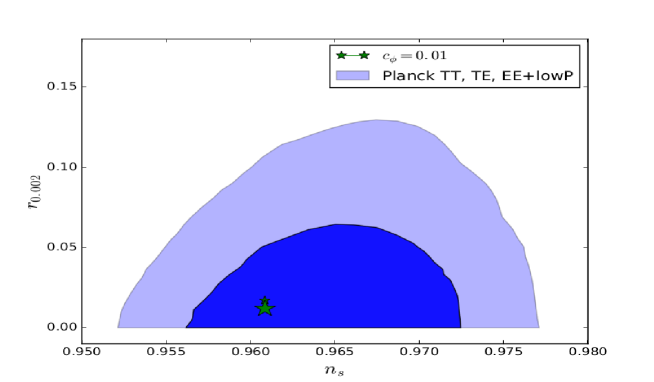
Figure 1: The $(n_{s},r)$ diagram for LQC with $\Gamma\propto T$ using $N=60$ (big star) and $N=50$ (small star). The $1\sigma$ and $2\sigma$ contours borrowed from Planck Ade:2015lrj .

Observational restrictions: The point of this section is to test the viability of LQC at the inflationary level, involving the latest CMB data. Concerning the number of e-folds we use $N=50$ and $N=60$ respectively. Overall, we find that for the current parametrizations of the dissipation parameter our $(n_{s},r)$ predictions satisfy the restrictions of Planck within $1\sigma$ uncertainties. For example, in figure 1 we present the $(n_{s},r)$ diagram which is provided by the Planck team. On top of that we plot the individual sets of $(n_{s},r)$ in LQC which is based on the dissipation parameter $\Gamma\propto T$. Evidently, our results are consistent with those of Planck. Regarding the scalar spectral index we find $n_{s}\simeq 0.962$ which is agreement with that of Planck $n_{s}=0.968\pm 0.006$. Lastly, as it can be viewed from figure 1, the tensor-to-scalar fluctuation ratio could reach the value of $r\simeq 0.02$ which is consistent within $1\sigma$ with that of BICEP2/KeckArray/Planck results Keck15 .

To summarize, the inflationary class of LQC models seems to accomplish two main achievements: i) it smoothly connects the Planck era with the CMB epoch; and ii) it leads to the same successful prediction compatible with the CMB parameters $(n_{s},r)$ provided by the Planck collaboration Ade:2015lrj ; Keck15 . Overall the combination of the recent work of Ashtekar and Gupt Gupt17 with the present Essay provides a complete investigation of LQC approach at the era of CMB.From both works it becomes clear that LQC, which is the outcome of the effective LQG theory, could provide an efficient way to understand the early phase of the universe.

References

- (1) P. A. R. Ade et al. [Planck Collaboration], [arXiv:1502.02114].
- (2) P. A. R. Ade et al. [BICEP2/Keck and Planck Collaborations], [arXiv:1502.0061]
- (3) A. Ashtekar and B. Gupt, Class. and Quant. Grav., 34, 014002 (2017)
- (4) M. Bojowald, Living Rev. Rel. 8, 11 (2005); A. Ashtekar and J. Lewandowski, Class. Quant. Grav. 21, R53 (2004); P. Singh and K. Vandersloot, Phys. Rev. D., 72, 084004 (2005)
- (5) A. Ashtekar, M. Bojowald, and J. Lewandowski, Adv. Theor. Math. Phys. 7, 233 (2003); A. Ashtekar, T. Pawlowski, and P. Singh, Phys. Rev. D,, 74, 084003 (2006)
- (6) P. Singh and K. Vandersloot, Phys. Rev. D., 04 (2005); A. Ashtekar, T. Pawlowski, and P. Singh, Phys. Rev. D., 73, 124038 (2006)
- (7) L.-F. Li and J.-Y. Zhu, Phys. Rev. D., 79, 124011 (2009),
- (8) G. W. Gibbons, Phys. Lett. B., 537 , 1 (2002)
- (9) S. del Campo, R. Herrera, and J. Saavedra, Eur. Phys.J. C. 59, 913 (2009); M. R. Setare and V. Kamali, JHEP 03, 066 (2013); X.-M. Zhang and J.-Y. Zhu, JCAP 1402, 005 (2014)
- (10) A. Berera, Phys. Rev. Lett., 75, 3218 (1995)
- (11) E. W. Kolb and M. S. Turner, Front. Phys., 69, 1 (1990)
- (12) L. M. H. Hall, I. G. Moss, and A. Berera, Phys. Rev. D., 69, 083525 (2004)
- (13) A. N. Taylor and A. Berera, Phys. Rev. D. 62, 083517 (2000)
- (14) Y. Zhang, JCAP, 0903, 023 (2009); M. Bastero-Gil, A. Berera, and R. O. Ramos, JCAP, 1107 , 030 (2011)
- (15) A. Berera, M. Gleiser, and R. O. Ramos, Phys. Rev. D. 58, 123508 (1998)
- (16) J. Yokoyama and A. D. Linde, Phys. Rev. D., 60, 083509 (1999); R. Herrera, M. Olivares, and N. Videla, Phys. Rev. D., 88, 063535 (2013)
- (17) A. Berera, I. G. Moss, and R. O. Ramos, Rept. Prog. Phys., 72, 026901 (2009); M. Bastero-Gil, A. Berera, R. O. Ramos, and J. G. Rosa, Phys. Rev. Lett., 117, 151301 (2016)