Comparison of variational balance models for the rotating shallow water equations

Abstract

We present an extensive numerical comparison of a family of balance models appropriate to the semi-geostrophic limit of the rotating shallow water equations, and derived by variational asymptotics in Oliver (2006) for small Rossby numbers ${\mathrm{Ro}}$. This family of generalized large-scale semi-geostrophic (GLSG) models contains the $L_{1}$-model introduced by Salmon (1983) as a special case. We use these models to produce balanced initial states for the full shallow water equations. We then numerically investigate how well these models capture the dynamics of an initially balanced shallow water flow. It is shown that, whereas the $L_{1}$-member of the GLSG family is able to reproduce the balanced dynamics of the full shallow water equations on time scales of ${\mathcal{O}}(1/{\mathrm{Ro}})$ very well, all other members develop significant unphysical high wavenumber contributions in the ageostrophic vorticity which spoil the dynamics.

Keywords: rotating shallow water, semi-geostrophic equations, balance models

1 Introduction

Atmospheric and oceanic large-scale flows are characterized by an approximate balance between Coriolis forces, buoyancy and pressure gradients. This balance causes large-scale features such as the high and low pressure fields which we experience as weather to vary only slowly, and also implies that faster processes such as inertia-gravity waves and acoustic waves are generally less important energetically.

Characterizing balance has been a longstanding problem in geophysical fluid dynamics. Four fundamental approaches are available. First, balance relations may be regarded as phase-space constraints in an asymptotic expansion of the equations of motion, in a distinguished limit of scaling parameters such as Rossby, Burger, and Froude number. Second, similarly, asymptotic expansions may be performed on the underlying Hamilton principle. Third, optimal balance strategies may be used to exploit the adiabatic invariance of the slow or balanced manifold under deformation (Viúdez & Dritschel, 2004). Fourth, time-filters may provide simple heuristics to distinguish balanced from imbalanced motion.

While balance models are clearly not sufficient as a dynamical core for contemporary weather or climate forecasting, there is continuing necessity to characterize, diagnose, and enforce balance in the context of such modeling. Respecting balance has long been recognized to be integral to the quality of weather forecasts. The first numerical weather forecast (albeit performed with pen and paper) by Richardson (1922) failed exactly because the initial fields used to seed the forecast were imbalanced, containing an excessive amount of small-scale high-frequency components, thereby spoiling the subsequent forecast (see the wonderful historical account in Lynch (2006)). In modern weather forecasting, the initial state is estimated by correcting the output from the forecast model, which may contain model error as well as instabilities, using information from noisy observations in a procedure called data assimilation. This procedure, however, typically does not respect balance, with the consequence that it may produce highly imbalanced initial states (Bloom et al., 1996; Mitchell et al., 2002; Ourmiéres et al., 2006; Kepert, 2009; Greybush et al., 2011; Gottwald, 2014).

Within the vast literature on asymptotic derivations of balance models, there are two main distinguished limits when the Rossby number, the ratio of typical advective time scales to the time scale of rotation, is small: (1) the quasi-geostrophic limit which assumes that the Burger number (see Section 2) remains of order one while variations in layer thickness are small, and (2) the semi-geostrophic limit which assumes that the Burger number remains small (comparable to the Rossby number) while variations in layer thickness may be order one. Quasi-geostrophy will not be considered further in this paper. The classic semi-geostrophic equations are based on the geostrophic momentum approximation (Eliassen, 1948) and were rewritten by Hoskins and solved via an ingenious change of coordinates (Hoskins, 1975; Cullen & Purser, 1984). They continue to attract interest due to their connection to optimal transport theory and the resulting possibility to make mathematical sense of generalized frontal-type solutions (Benamou & Brenier, 1998; Cullen, 2008). The geostrophic momentum approximation and Hoskins’ transformation inspired Salmon (1983, 1985) to make corresponding approximations directly to Hamilton’s principle so as to preserve geometrical structure and automatically preserve conservation laws.

In this paper, we perform a detailed numerical study of a particular family of asymptotic balance models, based on the generalized large-scale semi-geostrophic (GLSG) equations. These equations describe the motion of a rotating fluid in the limit of small Rossby and small Froude number, and here for simplicity we consider a single-layer shallow water flow only. The GLSG equations go back to an idea proposed by Salmon (1983, 1985). He suggested imposing a phase-space constraint directly in Hamilton’s principle, that is, in the variational derivation of the model equations. Oliver (2006) generalized this idea and derived a one-parameter family of balance models, the GLSG family, that includes the two models considered by Salmon as special cases. Each member of this family is characterized by a different choice of coordinates, and a transformation from these new coordinates into physical coordinates is given. For exactly one of these models, namely Salmon’s $L_{1}$-model, this transformation is so close to the identity that physical coordinates can be identified with model coordinates without changing the asymptotic order of the model, as is implicitly done in Salmon’s work.

The GLSG equations can be formulated in terms of potential vorticity advection and inversion, and can be shown to possess global smooth solutions (Çalık et al., 2013). Moreover, this family of models is distinct from other existing models in the semi-geostrophic limit such as those derived in Allen & Holm (1996), McIntyre & Roulstone (2002), and the so-called $\delta$-$\gamma$ balance model hierarchy of Mohebalhojeh & Dritschel (2001). The mathematical setting for this last group of models is less well investigated and we shall not consider them further in this paper.

Gottwald & Oliver (2014) proved, in a structurally analogous finite-dimensional context, that all models within the GLSG family provide the same asymptotic order of accuracy. In the infinite-dimensional fluid dynamical model context, a corresponding proof remains elusive. Moreover, it is already evident from an informal inspection of the resulting balance relations that the regularity provided by such relations for the constraint variables (or balanced variables) differs across the family of models. In fact, in one of the cases considered by Salmon (the $L_{1}$-model which emerges as the case $\lambda=\tfrac{1}{2}$ in the notation introduced below), the balance relation is an elliptic equation, in the other case (corresponding to $\lambda=-\tfrac{1}{2}$), the balance relation loses ellipticity and the resulting model is ill-posed as an initial value problem. Moreover, Oliver (2006) showed that the balance relation in a third special case (corresponding to $\lambda=0$) yields a velocity field that is more regular by at least two derivatives than any other member of the family. It has thus been an obvious question whether this apparent gain of regularity might be advantageous.

The main contribution of this paper is a careful comparative numerical evaluation of the GLSG family of balance models. Our main metric is a comparison of the balance model dynamics to a consistently initialized simulation of the full shallow water equations over a moderate interval of time chosen such that the Eulerian fields experience an order one relative change. We examine in particular the scaling behavior of the balance model error as the Rossby number goes to zero. Our numerical and mathematical analyses underscore the importance in understanding, and ensuring, the mathematical regularity of the balance relation underpinning any balance model. Crucially, our results show that it is the regularity of the ageostrophic components of the flow that has the greatest impact on how well the balance model is able to capture the dynamics of the full shallow water model. This singles out the $L_{1}$-model within the GLSG family of balance models as the only model with sufficient regularity on the ageostrophic vorticity to be viable in practice.

The paper is organized as follows. Section 2 presents the shallow water equations and their semi-geostrophic scaling. Section 3 briefly reviews the variational asymptotics by Oliver (2006) and re-expresses the GSLG balance relation in terms of ageostrophic variables. Section 4 describes the setup of our numerical experiments, including the details of the initialization procedure producing balanced initial conditions for the rotating shallow water equations. Section 5 present our results, showing that there exists a distinguished balance model, namely Salmon’s $L_{1}$-model, which produces reliably balanced states which remain near balance over times on which Eulerian fields evolve significantly. We conclude with a discussion and outlook in Section 6.

2 The shallow water equations and the semi-geostrophic limit

The simplest model of rapidly rotating fluid flow in which the idea of variational balance models can be tested is the rotating shallow water model. This describes the motion of a shallow layer of fluid of mean height $H$, held down by gravity $g$ and rotating uniformly at the rate $f/2$. The equations of motion (in the rotating frame of reference) consist of the momentum equation and the continuity equation, for the fluid velocity ${\boldsymbol{u}}=(u,v)$ and the height field $h$ (here, for convenience, scaled on $H$):

$$\partial_{t}{\boldsymbol{u}}+{\boldsymbol{u}}\boldsymbol{\cdot}\boldsymbol{\nabla}{\boldsymbol{u}}+f{\boldsymbol{u}}^{\bot}+c^{2}\,\boldsymbol{\nabla}h=0\,,$$ (1a)

$$\partial_{t}h+\boldsymbol{\nabla}\boldsymbol{\cdot}(h{\boldsymbol{u}})=0\,,$$ (1b)

where ${\boldsymbol{u}}^{\bot}=(v,-u)$ and $c^{2}=gH$ is the squared short-scale gravity wave speed. For simplicity, we consider flow in the doubly-periodic domain $\Omega=[0,2\pi]^{2}$.

Notably, the above equations imply material conservation of potential vorticity

$$q=\frac{f+\boldsymbol{\nabla}^{\bot}\boldsymbol{\cdot}{\boldsymbol{u}}}{h},$$ (2)

where $\boldsymbol{\nabla}^{\bot}\equiv(-\partial_{y},\partial_{x})$, that is

$$\partial_{t}q+{\boldsymbol{u}}\boldsymbol{\cdot}\boldsymbol{\nabla}q=0\,.$$ (3)

This is not an additional equation, but a consequence of combining (1a) and (1b). Alternatively, conservation of potential vorticity can be derived as a Noetherian conservation law from the particle-relabeling symmetry (Salmon, 1998).

Under appropriate rescaling, the shallow water equations are characterized by several dimensionless parameters. Taking $L$, $H$ and $U$ to be characteristic horizontal length, height and velocity scales, respectively, two parameters naturally emerge. The first is the Rossby number

$$\mathrm{Ro}=\frac{U}{fL}\,,$$ (4)

which measures the ratio of the relative vorticity $\zeta=\boldsymbol{\nabla}^{\bot}\boldsymbol{\cdot}{\boldsymbol{u}}$ of the fluid flow to the planetary vorticity (or Coriolis frequency) $f$. In the analysis below, we assume $\mathrm{Ro}\ll 1$. The second parameter is the Froude number

$$\mathrm{Fr}=\frac{U}{c}\,,$$ (5)

which measures the flow speed relative to the characteristic gravity wave speed $c=\sqrt{gH}$. This too is considered small. However, the ratio of these small parameters determines the flow regime observed. This is traditionally characterized by the Burger number

$$\mathrm{Bu}=\frac{\mathrm{Ro}^{2}}{\mathrm{Fr}^{2}}=\frac{L_{D}^{2}}{L^{2}}\,,$$ (6)

where $L_{D}=c/f$, known as the Rossby radius of deformation, signifies the length scale above which rotational effects dominate over buoyancy effects.

Here we consider semi-geostrophic scaling, for which $\mathrm{Bu}=\mathrm{Ro}$, in contrast to the more extensively studied quasi-geostrophic scaling, for which $\mathrm{Bu}={\mathcal{O}}(1)$ and height perturbations are of $\mathcal{O}(\mathrm{Ro})$ to maintain geostrophic balance at leading order. Notably, in semi-geostrophic scaling, (rescaled) height variations may be ${\mathcal{O}}(1)$.

The nondimensional equations are found by scaling $x$ and $y$ by $L$, ${\boldsymbol{u}}$ by $U$, $h$ by a mean height $H$, and $t$ by $L/U$. Defining $\varepsilon\equiv\mathrm{Ro}\ll 1$ as our small parameter and setting $\mathrm{Bu}=\varepsilon$, the equations become

$$\varepsilon\,(\partial_{t}{\boldsymbol{u}}+{\boldsymbol{u}}\boldsymbol{\cdot}\boldsymbol{\nabla}{\boldsymbol{u}})+{\boldsymbol{u}}^{\bot}+\boldsymbol{\nabla}h=0\,,$$ (7a)

$$\partial_{t}h+\boldsymbol{\nabla}\boldsymbol{\cdot}(h{\boldsymbol{u}})=0\,.$$ (7b)

The non-dimensional potential vorticity is

$$q=\frac{1+\varepsilon\,\boldsymbol{\nabla}^{\bot}\boldsymbol{\cdot}{\boldsymbol{u}}}{h}\,.$$ (8)

In the derivation of the GLSG balance models below, we will use the above non-dimensional form of the equations. Note, due to the rescaling adopted, the mean height $\bar{h}\equiv 1$.

3 A family of balance models

In this section, we give a brief review of the family of first-order generalized Lagrangian semi-geostrophic (GLSG) models which were derived in Oliver (2006). These models are asymptotic models for small Rossby number under semi-geostrophic scaling. Rather than performing asymptotics directly on the equations of motion (7), Oliver (2006) followed the strategy of Salmon (1983, 1998) and performed the asymptotics within the variational principle, thereby guaranteeing the conservation of the geometric Hamiltonian structure of the original shallow water equations.

3.1 A variational principle for shallow water

It is well known that the shallow water equations arise as the Euler–Lagrange equations from a variational principle; see, for example, Salmon (1983, 1998). In our opinion, it is most clearly presented using the following notation. We consistently write ${\boldsymbol{x}}$ to denote an Eulerian position and ${\boldsymbol{a}}$ to denote a Lagrangian label of a fluid parcel. The flow map ${\boldsymbol{\eta}}$ maps labels to Eulerian positions such that the parcel initially at location ${\boldsymbol{a}}$ is at location ${\boldsymbol{x}}={\boldsymbol{\eta}}({\boldsymbol{a}},t)$ at time $t$. We write ${\boldsymbol{u}}={\boldsymbol{u}}({\boldsymbol{x}},t)$ to denote the (Eulerian) velocity of the fluid at location ${\boldsymbol{x}}$ and time $t$. It equals the (Lagrangian) velocity of the parcel passing through ${\boldsymbol{x}}$ at time $t$, so that $\partial_{t}{\boldsymbol{\eta}}({\boldsymbol{a}},t)={\boldsymbol{u}}({\boldsymbol{\eta}}({\boldsymbol{a}},t),t)$, which we shall abbreviate

$$\dot{\boldsymbol{\eta}}={\boldsymbol{u}}\circ{\boldsymbol{\eta}}\,,$$ (9)

the symbol “$\circ$” denoting composition of maps with respect to the spatial variables. Liouville’s theorem states that the continuity equation (7b) is equivalent to

$$h\circ{\boldsymbol{\eta}}=\frac{h^{\operatorname{in}}}{\det\boldsymbol{\nabla}{\boldsymbol{\eta}}}\,,$$ (10)

where $h^{\operatorname{in}}=h^{\operatorname{in}}({\boldsymbol{a}})$ is the initial height field. To simplify the derivation of the equations of motion, we suppose for a moment that $h^{\operatorname{in}}=1$. This can be done without loss of generality because the equations of motion do not depend on the choice of the initial height field. With this convention, the layer depth is the Jacobian of the transformation from Eulerian to Lagrangian coordinates.

We can now introduce the Lagrangian

$$L =\int\bigl{[}({\boldsymbol{R}}+\tfrac{1}{2}\,\varepsilon\,{\boldsymbol{u}})\circ{\boldsymbol{\eta}}\boldsymbol{\cdot}\dot{\boldsymbol{\eta}}-\frac{1}{2}\,h\circ{\boldsymbol{\eta}}\bigr{]}\,{\mathrm{d}}{\boldsymbol{a}}$$

$$=\int h\,\bigl{[}{\boldsymbol{R}}\boldsymbol{\cdot}{\boldsymbol{u}}+\tfrac{1}{2}\,\varepsilon\,\lvert{\boldsymbol{u}}\rvert^{2}-\frac{1}{2}\,h\bigr{]}\,{\mathrm{d}}{\boldsymbol{x}}\,,$$ (11)

where ${\boldsymbol{R}}$ denotes the vector potential corresponding to the Coriolis parameter, such that $\boldsymbol{\nabla}^{\bot}\boldsymbol{\cdot}{\boldsymbol{R}}=f\equiv 1$. It is not hard to show that the shallow water equations (7) arise as the stationary points of the action

$$S=\int_{t_{1}}^{t_{2}}L[{\boldsymbol{u}},h]\,{\mathrm{d}}t$$ (12)

with respect to variations of the flow map ${\boldsymbol{\eta}}$. Since $h$ and ${\boldsymbol{u}}$ are linked to ${\boldsymbol{\eta}}$ by relations (9) and (10) above, variations in ${\boldsymbol{\eta}}$ induce variations in $h$ and ${\boldsymbol{u}}$ of a specific form. This is most easily expressed by noting that a variation of the flow map $\delta{\boldsymbol{\eta}}$ can be thought of as induced by an Eulerian vector field ${\boldsymbol{w}}={\boldsymbol{w}}({\boldsymbol{x}})$ via

$$\delta{\boldsymbol{\eta}}={\boldsymbol{w}}\circ{\boldsymbol{\eta}}\,,$$ (13)

a direct analog to relation (9). Just the same, there holds a Liouville theorem with respect to a parametrization of the variation, which implies the “continuity equation”

$$\delta h+\boldsymbol{\nabla}\boldsymbol{\cdot}({\boldsymbol{w}}h)=0\,.$$ (14)

Finally, cross-differentiation of (9) and (13) yields the so-called Lin constraint (Bretherton, 1970):

$$\delta{\boldsymbol{u}}=\dot{\boldsymbol{w}}+\boldsymbol{\nabla}{\boldsymbol{w}}\,{\boldsymbol{u}}-\boldsymbol{\nabla}{\boldsymbol{u}}\,{\boldsymbol{w}}\,.$$ (15)

The remainder of the derivation proceeds by direct computation and shall be omitted. We remark, however, that the argument requires that the Coriolis parameter $f$ can be written as the curl of a vector potential. On the plane, this is easy to achieve. However, on the torus, $f$ has a vector potential if and only if it has zero mean, thereby excluding the case of a constant Coriolis parameter considered here. However, a careful inspection of the problem shows that if we proceed as if the vector potential ${\boldsymbol{R}}$ existed, we would obtain equations of motion which are Hamiltonian in the expected sense, but strictly speaking do not arise as the Euler–Lagrange equations of a variational principle. A detailed discussion of this issue is given in Oliver & Vasylkevych (2011). We shall henceforth ignore this subtlety as it is not pertinent to the main point of this paper.

3.2 Variational asymptotics

The key idea introduced in Oliver (2006) is to introduce a new coordinate system which is related to the original coordinate system by an ${\mathcal{O}}(\varepsilon)$ perturbation of the identity in such a way that the first-order transformed Lagrangian becomes degenerate. As a result, truncation of the Lagrangian to first order leads to Euler–Lagrange equations which live on a reduced phase space.

To systematically develop this idea, it is convenient to view the transformation itself as a flow parametrized by $\varepsilon$. Concretely, we shall endow quantities in the original (physical) coordinate system with a subscript $\varepsilon$, while quantities without subscript shall be viewed as posed in a new, slightly distorted coordinate system. (This choice makes the transformation from new to old coordinates explicit, while the transformation from old to new coordinates is implicit.) We view the transformation as being generated by a vector field ${\boldsymbol{v}}_{\varepsilon}$ via

$${\boldsymbol{\eta}}_{\varepsilon}^{\prime}={\boldsymbol{v}}_{\varepsilon}\circ{\boldsymbol{\eta}}_{\varepsilon}\,,$$ (16)

where the prime denotes a derivative with respect to $\varepsilon$ and ${\boldsymbol{\eta}}_{0}\equiv{\boldsymbol{\eta}}$. Once more, we have a continuity equation which now reads

$$h_{\varepsilon}^{\prime}+\boldsymbol{\nabla}\boldsymbol{\cdot}({\boldsymbol{v}}_{\varepsilon}h_{\varepsilon})=0\;,$$ (17)

and an analog of the Lin constraint (15),

$${\boldsymbol{u}}_{\varepsilon}^{\prime}=\dot{\boldsymbol{v}}_{\varepsilon}+\boldsymbol{\nabla}{\boldsymbol{v}}_{\varepsilon}\,{\boldsymbol{u}}_{\varepsilon}-\boldsymbol{\nabla}{\boldsymbol{u}}_{\varepsilon}\,{\boldsymbol{v}}_{\varepsilon}\,.$$ (18)

In the following, we shall denote the formal Taylor coefficients of ${\boldsymbol{u}}_{\varepsilon}$ with respect to an expansion in $\varepsilon$ by ${\boldsymbol{u}}$, ${\boldsymbol{u}}^{\prime}$, etc., with analogous notation for all other quantities.

In summary, altogether we are considering a three parameter family of flow maps, the parameters being physical time $t$, asymptotic parameter $\varepsilon$, and an implicit parameter in the definition of the variational derivative. Structurally, these parameters play entirely symmetric roles, the difference lies in their physical interpretation. Each Lagrangian-parameter derivative has an associated Eulerian vector field: ${\boldsymbol{u}}_{\varepsilon}$ for the time derivative, ${\boldsymbol{v}}_{\varepsilon}$ for the $\varepsilon$-derivative, and ${\boldsymbol{w}}_{\varepsilon}$ for the variational derivative. We can interpret ${\boldsymbol{v}}_{\varepsilon}$ as the velocity of deformation of the coordinate system in “artificial time” $\varepsilon$, and ${\boldsymbol{w}}_{\varepsilon}$ as the Eulerian version of the virtual displacement in classical mechanics (e.g. Goldstein 1980). The definition of $h_{\varepsilon}$ as the inverse Jacobian of the map ${\boldsymbol{\eta}}_{\varepsilon}$ implies a continuity equation in each of these parameters, stated in (7b), (17), and (14), respectively. Mixed derivatives satisfy generalized Lin constraints such as (15) and (18).

We now proceed to expand the Lagrangian (11) in powers of $\varepsilon$:

$$L_{\varepsilon}=\int\bigl{[}{\boldsymbol{R}}\circ{\boldsymbol{\eta}}\boldsymbol{\cdot}\dot{\boldsymbol{\eta}}-\frac{1}{2}\,h\circ{\boldsymbol{\eta}}\bigr{]}\,{\mathrm{d}}{\boldsymbol{a}}+\varepsilon\,\int\bigl{[}{\boldsymbol{v}}^{\bot}\boldsymbol{\cdot}{\boldsymbol{u}}+\tfrac{1}{2}\,\lvert{\boldsymbol{u}}\rvert^{2}+\frac{1}{2}\,h\,\boldsymbol{\nabla}\boldsymbol{\cdot}{\boldsymbol{v}}\bigr{]}\circ{\boldsymbol{\eta}}\,{\mathrm{d}}{\boldsymbol{a}}+{\mathcal{O}}(\varepsilon^{2})\,.$$ (19)

Details of this calculation can be found in Appendix B of Oliver (2006). The transformation vector field ${\boldsymbol{v}}$ at ${\mathcal{O}}(\varepsilon)$ may be chosen arbitrarily. Clearly, any choice of the form

$${\boldsymbol{v}}=\tfrac{1}{2}\,{\boldsymbol{u}}^{\bot}+{\boldsymbol{F}}(h)$$ (20)

renders the first-order Lagrangian $L_{1}$ affine (i.e., it is linear in the velocity and thus degenerate). The dimensionally consistent choice

$${\boldsymbol{v}}=\tfrac{1}{2}\,{\boldsymbol{u}}^{\bot}+\lambda\,\boldsymbol{\nabla}h$$ (21)

leads to a particular one-parameter family of balance models — when the system is in geostrophic balance, the second term is a scalar multiple of the first. In this setting, the choice $\lambda=\tfrac{1}{2}$ emerges as a special case: at leading order, both terms cancel so that, formally, ${\boldsymbol{v}}=\mathcal{O}(\varepsilon)$.

Inserting the choice (21) back into (19) and dropping terms of order ${\mathcal{O}}(\varepsilon^{2})$, we obtain

$$L_{\operatorname{bal}}=\int\bigl{[}{\boldsymbol{R}}+\varepsilon\,(\lambda+\tfrac{1}{2})\,\boldsymbol{\nabla}^{\bot}h\bigr{]}\circ{\boldsymbol{\eta}}\boldsymbol{\cdot}\dot{\boldsymbol{\eta}}\,{\mathrm{d}}{\boldsymbol{a}}-\int h\,\bigl{[}\tfrac{1}{2}\,h+\varepsilon\,\lambda\,\lvert\boldsymbol{\nabla}h\rvert^{2}\bigr{]}\,{\mathrm{d}}{\boldsymbol{x}}\,,$$ (22)

where, for convenience, we have written the part which is linear in ${\boldsymbol{u}}$ as an integral over labels and the part which only depends on $h$ as an integral over Eulerian positions.

For the convenience of the reader, the explicit variational calculus of $L_{\operatorname{bal}}$ is presented in Appendix A. The stationary points of the action necessitate the Euler–Lagrange equation

$$\bigl{[}1-\varepsilon\,(\lambda+\tfrac{1}{2})\,(h\,\Delta+2\,\boldsymbol{\nabla}h\boldsymbol{\cdot}\boldsymbol{\nabla})\bigr{]}{\boldsymbol{u}}=\boldsymbol{\nabla}^{\bot}\bigl{[}h-\varepsilon\,\lambda\,(2\,h\,\Delta h+\lvert\boldsymbol{\nabla}h\rvert^{2})\bigr{]}\,,$$ (23)

where $\Delta$ denotes Laplace’s operator. For a given nonnegative height field $h$, this equation is a non-constant coefficient elliptic equation for ${\boldsymbol{u}}$ when $\lambda>-\frac{1}{2}$. This constitutes the family of balance relations, parametrized by the free parameter $\lambda$.

The system of equations for the balance model can be closed via the continuity equation

$$\partial_{t}h+\boldsymbol{\nabla}\boldsymbol{\cdot}(h{\boldsymbol{u}})=0\,.$$ (24)

By construction, the balance model has a conserved energy,

$$H_{\operatorname{bal}}=\frac{1}{2}\int h^{2}\,{\mathrm{d}}{\boldsymbol{x}}+\varepsilon\,\lambda\int h\,\lvert\boldsymbol{\nabla}h\rvert^{2}\,{\mathrm{d}}{\boldsymbol{x}}\,,$$ (25)

and a materially conserved potential vorticity

$$q=\frac{1+\varepsilon\,(\lambda+\frac{1}{2})\,\Delta h}{h}\,.$$ (26)

Thus, we can choose either (24) or the potential vorticity conservation law

$$\partial_{t}q+{\boldsymbol{u}}\boldsymbol{\cdot}\boldsymbol{\nabla}q=0$$ (27)

to evolve the balance relation (23) in time. This equivalence can be checked by brute-force computation, or by noting that potential vorticity advection is the natural conservation law associated with the particle relabeling symmetry in the variational derivation of the balanced models (Oliver, 2006). If we opt for $q$ as the fundamental prognostic variable, the height field $h$ can be recovered by inversion of (26) via

$$\bigl{(}q-\varepsilon\,(\lambda+\tfrac{1}{2})\Delta\bigr{)}h=1\,,$$ (28)

after which ${\boldsymbol{u}}$ is computed from $h$ via (23). Thus, (27), (28), and (23) form a closed system for the balanced dynamics. This formulation is used numerically and also underlies the proof of global well-posedness (Çalık et al., 2013) and of global existence of weak solutions (Çalık & Oliver, 2013) for the family of balance models.

Note that, to leading order, the motion induced by a velocity field computed from (23) is geostrophic with an ${\mathcal{O}}(1)$ velocity. Thus, fluid parcels travel a unit distance over times of ${\mathcal{O}}(1)$. The rate of change of the Eulerian fields, on the other hand, is determined by the magnitude of the ageostrophic velocity which is ${\mathcal{O}}(\varepsilon)$, independent of $\lambda$. (An explicit formal calculation can be found in Appendix B.) Thus, to test the prognostic skill of the balance model, we need to simulate on time scales of order ${\mathcal{O}}(\varepsilon^{-1})$.

3.3 Balance relation in $\delta$-$\gamma$ variables

For the understanding of the behavior of the balance relation for different values of the free parameter $\lambda$, it is crucial to look at the effect of the balance relation on the ageostrophic velocity in balance model coordinates,

$${\boldsymbol{u}}^{\operatorname{ag}}={\boldsymbol{u}}-\boldsymbol{\nabla}^{\bot}h\,.$$ (29)

We choose to re-express the ageostrophic motion in terms of the balance model divergence $\delta=\boldsymbol{\nabla}\boldsymbol{\cdot}{\boldsymbol{u}}$ and ageostrophic vorticity $\gamma=\boldsymbol{\nabla}^{\bot}\boldsymbol{\cdot}{\boldsymbol{u}}^{\operatorname{ag}}=\boldsymbol{\nabla}^{\bot}\boldsymbol{\cdot}{\boldsymbol{u}}-\Delta h$. Strictly speaking, the ageostrophic vorticity is better described as the acceleration divergence since, for the full shallow water equations, $\gamma=\boldsymbol{\nabla}\boldsymbol{\cdot}(\partial_{t}{\boldsymbol{u}}+{\boldsymbol{u}}\boldsymbol{\cdot}\boldsymbol{\nabla}{\boldsymbol{u}})$ via the shallow water momentum equation and this characterization remains appropriate in spherical geometry (Smith & Dritschel, 2006). Nevertheless, in the following we shall refer to $\gamma$ as the ageostrophic vorticity.

We now rewrite the balance relation in terms of $\delta$ and $\gamma$ by taking the divergence and curl of (23), obtaining

$$\bigl{[}1-\varepsilon\,(\lambda+\tfrac{1}{2})\,(h\,\Delta+2\,\boldsymbol{\nabla}h\boldsymbol{\cdot}\boldsymbol{\nabla})\bigr{]}\delta=\varepsilon\,(\lambda+\tfrac{1}{2})\,(\boldsymbol{\nabla}h\boldsymbol{\cdot}\Delta{\boldsymbol{u}}+2\,\boldsymbol{\nabla}\boldsymbol{\nabla}h:\boldsymbol{\nabla}{\boldsymbol{u}})$$ (30a)

and

$$\bigl{[}1-\varepsilon\,(\lambda+\tfrac{1}{2})\,(h\,\Delta+2\,\boldsymbol{\nabla}h\boldsymbol{\cdot}\boldsymbol{\nabla})\bigr{]}\gamma=\varepsilon\,(\lambda+\tfrac{1}{2})\,(\boldsymbol{\nabla}^{\bot}h\boldsymbol{\cdot}\Delta{\boldsymbol{u}}+2\,\boldsymbol{\nabla}\boldsymbol{\nabla}^{\bot}h:\boldsymbol{\nabla}{\boldsymbol{u}})\\ +\varepsilon\,(\tfrac{1}{2}-\lambda)\,h\,\Delta^{2}h+\varepsilon\,(1-4\lambda)\,\boldsymbol{\nabla}h\boldsymbol{\cdot}\boldsymbol{\nabla}\Delta h-2\varepsilon\lambda\,((\Delta h)^{2}+\lvert\boldsymbol{\nabla}\boldsymbol{\nabla}h\rvert^{2})\,,$$ (30b)

where $A:B$ denotes the matrix inner product $A:B=\sum_{i,j}a_{ij}\,b_{ij}$. To eliminate all references to ${\boldsymbol{u}}$ on the right hand sides, we decompose ${\boldsymbol{u}}$ into its rotational and divergent components by writing

$${\boldsymbol{u}}=\boldsymbol{\nabla}^{\bot}\psi+\boldsymbol{\nabla}\phi$$ (31)

so that

$$\psi=\Delta^{-1}\gamma+h\qquad\text{and}\qquad\phi=\Delta^{-1}\delta\,.$$ (32)

Then

$$\boldsymbol{\nabla}^{\bot}h\boldsymbol{\cdot}\Delta{\boldsymbol{u}}=\boldsymbol{\nabla}h\boldsymbol{\cdot}\Delta\boldsymbol{\nabla}h+\boldsymbol{\nabla}h\boldsymbol{\cdot}\boldsymbol{\nabla}\gamma+\boldsymbol{\nabla}^{\bot}h\boldsymbol{\cdot}\boldsymbol{\nabla}\delta$$ (33)

and

$$\boldsymbol{\nabla}\boldsymbol{\nabla}^{\bot}h:\boldsymbol{\nabla}{\boldsymbol{u}}=\lvert\boldsymbol{\nabla}\boldsymbol{\nabla}h\rvert^{2}+\boldsymbol{\nabla}\boldsymbol{\nabla}h:\boldsymbol{\nabla}\boldsymbol{\nabla}\Delta^{-1}\gamma+\boldsymbol{\nabla}\boldsymbol{\nabla}^{\bot}h:\boldsymbol{\nabla}\boldsymbol{\nabla}\Delta^{-1}\delta\,,$$ (34)

with similar relations for the terms on the right hand side of (30a). Inserting these expressions back into (30) and rearranging terms, we obtain

$$\bigl{(}1 -\varepsilon\,(\lambda+\tfrac{1}{2})\,h\,\Delta\bigr{)}\delta=\varepsilon\,(\lambda+\tfrac{1}{2})\,\boldsymbol{\nabla}h\boldsymbol{\cdot}\boldsymbol{\nabla}^{\bot}\Delta h$$

$$\quad+\varepsilon\,(\lambda+\tfrac{1}{2})\,\bigl{(}\boldsymbol{\nabla}h\boldsymbol{\cdot}\boldsymbol{\nabla}^{\bot}\gamma+2\,\boldsymbol{\nabla}\boldsymbol{\nabla}h:\boldsymbol{\nabla}\boldsymbol{\nabla}^{\bot}\Delta^{-1}\gamma+3\,\boldsymbol{\nabla}h\boldsymbol{\cdot}\boldsymbol{\nabla}\delta+2\,\boldsymbol{\nabla}\boldsymbol{\nabla}h:\boldsymbol{\nabla}\boldsymbol{\nabla}\Delta^{-1}\delta\bigr{)}$$ (35a)

and

$$\bigl{(}1 -\varepsilon\,(\lambda+\tfrac{1}{2})\,h\,\Delta\bigr{)}\gamma=-2\varepsilon\,\det\operatorname{Hess}h$$

$$\quad+\varepsilon\,(\tfrac{1}{2}+\lambda)\,\bigl{(}3\,\boldsymbol{\nabla}h\boldsymbol{\cdot}\boldsymbol{\nabla}\gamma+2\,\boldsymbol{\nabla}\boldsymbol{\nabla}h:\boldsymbol{\nabla}\boldsymbol{\nabla}\Delta^{-1}\gamma+\boldsymbol{\nabla}^{\bot}h\boldsymbol{\cdot}\boldsymbol{\nabla}\delta+2\,\boldsymbol{\nabla}\boldsymbol{\nabla}^{\bot}h:\boldsymbol{\nabla}\boldsymbol{\nabla}\Delta^{-1}\delta\bigr{)}$$

$$\quad+\varepsilon\,(\tfrac{1}{2}-\lambda)\,\bigl{(}h\,\Delta^{2}h+3\,\boldsymbol{\nabla}h\boldsymbol{\cdot}\boldsymbol{\nabla}\Delta h+2\,(\Delta h)^{2}\bigr{)}\,.$$ (35b)

The operator on the left-hand sides is elliptic for $\lambda>-\tfrac{1}{2}$. The terms in each of the second lines are linear in $\delta$ or $\gamma$, hence are formally of ${\mathcal{O}}(\varepsilon^{2})$. Thus, at least when $\lambda=\tfrac{1}{2}$, the dominant contribution comes from the first term on each right hand side.

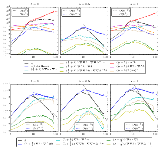
However, when $\lambda\neq\tfrac{1}{2}$, the right hand side of balance relation (35b) features additional terms involving third and fourth-order derivatives of $h$, alongside second-order derivatives. Thus, the regularity of the ageostrophic vorticity is severely reduced unless $\lambda=\tfrac{1}{2}$. Our numerical results show that this loss of regularity, which affects the balance relation for $\gamma$ only, has significant detrimental effects on the prognostic skill of the balance model, as discussed in detail in Sections 5.4–5.5 below.

Our numerical results further show that the dominant right hand term in the balance relation for $\delta$ (35a), namely $\boldsymbol{\nabla}h\boldsymbol{\cdot}\boldsymbol{\nabla}^{\bot}\Delta h$ shown as the blue curve in the bottom row of Figure 10, appears more regular than the the corresponding term in the balance relation for $\gamma$ (35b), namely $\boldsymbol{\nabla}h\boldsymbol{\cdot}\boldsymbol{\nabla}\Delta h$ shown as the magenta curve on the top row of Figure 10. The cause of the apparent cancellations in the former term is currently not understood.

3.4 Transformation to shallow water coordinates

Since the balance model dynamics, for each of the models introduced above, is posed in a coordinate frame different from the physical frame of the full shallow water dynamics, we need to apply a coordinate transformation for consistent initialization and diagnostics. The transformation between the two is explicit going from model coordinates to physical coordinates. Its inverse is defined implicitly and will generally involve an infinite series in $\varepsilon$. Therefore, except for the case of the $L_{1}$ model, it is not possible to write out the balance model in physical coordinates.

For consistent initialization and diagnostics of our numerical tests, we need to write out the change of coordinates explicitly. As we are only carrying terms to ${\mathcal{O}}(\varepsilon)$, we have

$$h_{\varepsilon}=h+\varepsilon\,h^{\prime}\qquad\text{and}\qquad{\boldsymbol{u}}_{\varepsilon}={\boldsymbol{u}}+\varepsilon{\boldsymbol{u}}^{\prime}$$ (36)

with

$$h^{\prime}=-\boldsymbol{\nabla}\boldsymbol{\cdot}({\boldsymbol{v}}h)\,,$$ (37a)

$${\boldsymbol{u}}^{\prime}=\dot{\boldsymbol{v}}+\boldsymbol{\nabla}{\boldsymbol{v}}\,{\boldsymbol{u}}-\boldsymbol{\nabla}{\boldsymbol{u}}\,{\boldsymbol{v}}\,,$$ (37b)

where

$${\boldsymbol{v}}=\tfrac{1}{2}\,{\boldsymbol{u}}^{\bot}+\lambda\,\boldsymbol{\nabla}h\,,$$ (38)

and where ${\boldsymbol{u}}$ and $h$ satisfy the balance relation (23). We then compute the shallow water potential vorticity, divergence, and ageostrophic vorticity via

$$q_{\varepsilon}=(1+\boldsymbol{\nabla}^{\bot}\cdot{\boldsymbol{u}}_{\varepsilon})/h_{\varepsilon}\,,\qquad\delta_{\varepsilon}=\boldsymbol{\nabla}\boldsymbol{\cdot}{\boldsymbol{u}}_{\varepsilon}\,,\qquad\text{and}\qquad\gamma_{\varepsilon}=\boldsymbol{\nabla}^{\bot}\boldsymbol{\cdot}{\boldsymbol{u}}_{\varepsilon}-\Delta h_{\varepsilon}\,.$$ (39)

When presenting our results, we will use the suggestive notation $\operatorname{T}[q]$, $\operatorname{T}[\delta]$, and $\operatorname{T}[\gamma]$ for the fields obtained via transformation from the balance model quantities, with the understanding that this notation does not imply any strict functional dependence — all of these transformed quantities are functionally dependent only on the balance model potential vorticity $q$.

The transformation from physical coordinates to balance model coordinates cannot be written down explicitly. However, it is possible to numerically invert the transformation for moderate values of the characteristic parameters using an iterative scheme sketched in Appendix C.

We finally remark that the transformation involves taking time derivatives of ${\boldsymbol{u}}$ and $h$. Formally, these terms are ${\mathcal{O}}(\varepsilon)$ as verified in Appendix B. Moreover, when $\lambda=\tfrac{1}{2}$, then ${\boldsymbol{v}}$ itself is ${\mathcal{O}}(\varepsilon)$ and the transformation remains ${\mathcal{O}}(\varepsilon^{2})$ — and thus coincides with the identity up to the formal order of validity of the balance model. Practically, this means that the transformation can be omitted when $\lambda=\tfrac{1}{2}$, i.e. the fields of the balanced equations and of the full shallow water equations can be directly compared without affecting the formal order of accuracy. We have numerically verified that the effect of the transformation is indeed negligible for this particular case; our detailed results, however, are computed with the transformation applied for all values of $\lambda$.

We stress that the GLSG balance models consist of both the prognostic equation (23) with assocated potential vorticity inversion (27) and (28), and the near-identity transformation relating the balance model solution to the corresponding quantities in a physical coordinate frame. When transformed back to physical coordinates, all the models considered here have the same $\mathcal{O}(\varepsilon)$ order of accuracy at least formally, the only difference being that the transformation is necessary to maintain order when $\lambda\neq\tfrac{1}{2}$. In finite dimensions, this statement is rigorous (Gottwald & Oliver, 2014). In the present setting, loss of accuracy can only be due to analytical issues in infinite dimensions, not due to an inconsistent handling of terms in the formal expansion. We note, in particular, that the transformed balance model potential vorticity given by (39) coincides with the shallow water potential vorticity (8) up to terms of $\mathcal{O}(\varepsilon^{2})$ for all values of $\lambda$. Similarly, the balanced model Hamiltonian, transformed back to physical coordinates, coincides with the shallow water Hamiltonian up to terms of $\mathcal{O}(\varepsilon^{2})$ for all values of $\lambda$.

4 Experimental setup

4.1 Benchmarking scheme

We now describe the details of our benchmarking procedure to determine how well the different GLSG balance models are able to describe nearly balanced shallow water dynamics. For a fixed value of the parameter $\lambda$, we go through the following steps:

1. At time $t=0$, specify the initial balance model height field $h^{\operatorname{in}}$.

2. On the balance model side, compute the initial balance model potential vorticity $q^{\operatorname{in}}$ using (26).

3. Compute the initial shallow water $q_{\varepsilon}^{\operatorname{in}}=\operatorname{T}[q^{\operatorname{in}}]$, $\delta_{\varepsilon}^{\operatorname{in}}=\operatorname{T}[\delta^{\operatorname{in}}]$, and $\gamma_{\varepsilon}^{\operatorname{in}}=\operatorname{T}[\gamma^{\operatorname{in}}]$ via the equations detailed in Section 3.4.

4. Evolve the balance model potential vorticity $q$ to some final state $q({\boldsymbol{x}},t)$ at time $t$ using (27). The balance model height field $h$ and velocity field ${\boldsymbol{u}}$ are kinematically slaved to $q$ via (28) and (23), respectively, and computed as part of the forward evolution.

5. Evolve the shallow water fields $q_{\varepsilon}$, $\delta_{\varepsilon}$, and $\gamma_{\varepsilon}$ to the same final time $t=1/\varepsilon$.

6. Transform the balance model state, at any chosen time, to shallow water coordinates as detailed in Section 3.4; compare $q_{\varepsilon}$ with $\operatorname{T}[q]$, $\delta_{\varepsilon}$ with $\operatorname{T}[\delta]$, and $\gamma_{\varepsilon}$ with $\operatorname{T}[\gamma]$.

It is also possible to initialize on the shallow water side, i.e. given only the initial distribution of shallow water potential vorticity $q_{\varepsilon}^{\operatorname{in}}$, see Appendix C. This is more demanding computationally, but does not affect any of our conclusions. Such an initialization may be useful for quantifying the amount of imbalance (or departure from balance) occurring over the course of a shallow water simulation. This however is not the aim of the present study; instead we seek to determine how well balance models can predict a shallow water flow evolution.

4.2 The shallow water equations in $q$-$\delta$-$\gamma$ coordinates

The shallow water model requires additional care since in this case there are three prognostic variables, not one as in the balance model. In the shallow water model we employ potential vorticity $q_{\varepsilon}$, divergence $\delta_{\varepsilon}$ and ageostrophic vorticity $\gamma_{\varepsilon}$ rather than more traditional choices like $h_{\varepsilon}$, $u_{\varepsilon}$, and $v_{\varepsilon}$, or like $h_{\varepsilon}$, $\zeta_{\varepsilon}$, and $\delta_{\varepsilon}$. Previous work has shown that $q_{\varepsilon}$, $\delta_{\varepsilon}$, and $\gamma_{\varepsilon}$ offer significant advantages over traditional variable choices (Mohebalhojeh & Dritschel, 2001, 2004). In particular, they offer significantly greater accuracy in the representation of both the balanced and imbalanced parts of the flow. Moreover, $q_{\varepsilon}$, $\delta_{\varepsilon}$, and $\gamma_{\varepsilon}$ lead to linear elliptic problems to determine $h_{\varepsilon}$ and ${\boldsymbol{u}}_{\varepsilon}$, advantageous for both numerical robustness and efficiency.

Ignoring hyperviscosity, the prognostic equations for $\delta_{\varepsilon}$ and $\gamma_{\varepsilon}$ (in dimensional terms) are

$$\partial_{t}\delta_{\varepsilon}=\gamma_{\varepsilon}+2\,J(u_{\varepsilon},v_{\varepsilon})-\boldsymbol{\nabla}\boldsymbol{\cdot}({\boldsymbol{u}}_{\varepsilon}\delta_{\varepsilon})\,,$$ (40a)

$$\partial_{t}\gamma_{\varepsilon}=-f^{2}\,\delta_{\varepsilon}+c^{2}\,\Delta\boldsymbol{\nabla}\boldsymbol{\cdot}({\boldsymbol{u}}_{\varepsilon}h_{\varepsilon})-f\,\boldsymbol{\nabla}\boldsymbol{\cdot}({\boldsymbol{u}}_{\varepsilon}\zeta_{\varepsilon})\,,$$ (40b)

where $J(a,b)=\partial_{x}a\,\partial_{y}b-\partial_{y}a\,\partial_{x}b$, and $\zeta_{\varepsilon}=h_{\varepsilon}q_{\varepsilon}-f$ is the relative vorticity.

The fields $\delta_{\varepsilon}$, $\gamma_{\varepsilon}$, and $q_{\varepsilon}$ determine the velocity field ${\boldsymbol{u}}_{\varepsilon}$ only up to a spatially independent mean flow $\bar{{\boldsymbol{u}}}_{\varepsilon}(t)$. In general, this flow is non-zero, though typically of very small amplitude (we have checked that in the numerical simulations presented below the mean flow has an amplitude of about $10^{-4}\,\lvert{\boldsymbol{u}}_{\varepsilon}\rvert_{\rm{max}}$). It is taken into account not only for completeness but to ensure an accurate assessment of the differences between the shallow water and the transformed balance flow solutions. To write out the evolution equation for $\bar{{\boldsymbol{u}}}_{\varepsilon}(t)$, we take the average of (1a):

$$\partial_{t}\bar{\boldsymbol{u}}_{\varepsilon}=-\overline{(f+\zeta_{\varepsilon})\,{\boldsymbol{u}}_{\varepsilon}^{\bot}}=-\overline{h_{\varepsilon}q_{\varepsilon}{\boldsymbol{u}}_{\varepsilon}^{\bot}}\,.$$ (41)

These additional two ordinary differential equations complete the set of prognostic equations of the $q$-$\delta$-$\gamma$ formulation of the shallow water equations. The initial mean flow is determined as the spatial average of the initial velocity field which is available via the transformation from balance model coordinates.

From $\delta_{\varepsilon}$, $\gamma_{\varepsilon}$, and $q_{\varepsilon}$, the fields $h_{\varepsilon}$ and $\hat{\boldsymbol{u}}_{\varepsilon}$, the mean-free component of ${\boldsymbol{u}}_{\varepsilon}$, are recovered by linear inversion. First, the definition $\gamma_{\varepsilon}=f\,\zeta_{\varepsilon}-c^{2}\,\Delta h_{\varepsilon}$, the definition of $\zeta_{\varepsilon}$, and the normalization of the mean height $\bar{h}_{\varepsilon}\equiv 1$ (see Section 2) lead to

$$c^{2}\,\Delta\hat{h}_{\varepsilon}-f\,q_{\varepsilon}\hat{h}_{\varepsilon}=-\gamma_{\varepsilon}-f^{2}+f\,q_{\varepsilon}\,,$$ (42)

a linear elliptic equation for $\hat{h}_{\varepsilon}$, the mean-free component of $h_{\varepsilon}$. Then, once $h_{\varepsilon}=\hat{h}_{\varepsilon}+1$ is determined, $\hat{\boldsymbol{u}}_{\varepsilon}$ is simply found using the Helmholtz decomposition $\hat{\boldsymbol{u}}_{\varepsilon}=\boldsymbol{\nabla}^{\perp}\psi_{\varepsilon}+\boldsymbol{\nabla}\phi_{\varepsilon}$. This results in the Poisson equations $\Delta\psi_{\varepsilon}=\zeta_{\varepsilon}$ and $\Delta\phi_{\varepsilon}=\delta_{\varepsilon}$, both of which are directly solved in spectral space. The velocity $\hat{\boldsymbol{u}}_{\varepsilon}$ is then found by differentiation of $\psi_{\varepsilon}$ and $\phi_{\varepsilon}$, and ${\boldsymbol{u}}_{\varepsilon}=\hat{\boldsymbol{u}}_{\varepsilon}+\bar{\boldsymbol{u}}_{\varepsilon}$.

4.3 Implementation

The numerical models developed for the shallow water and balance equations, including all initialization and diagnostic procedures, make use of the standard pseudo-spectral method in doubly-periodic geometry. In this method, nonlinear products are carried out in physical space (on a regular grid), while all linear operations such as differentiation and inversion are carried out in spectral space. Fast Fourier transforms are used to go from one representation to the other.

To minimize aliasing errors, prior to carrying out nonlinear products, fields are spectrally truncated using a circular filter of radius (wavenumber magnitude) $k=n_{\rm g}/3$ where $n_{\rm g}$ is the grid resolution in both $x$ and $y$ (here the domain is square with side length $2\pi$ without loss of generality). Note, the maximum wavenumber is $k_{\rm{max}}=n_{\rm g}/2$. We use $n_{\rm g}=256$ throughout but have verified that $n_{\rm g}=512$ does not change the results significantly in a sample of cases. While proper de-aliasing would remove more modes, the circular filter adopted better preserves isotropy and has been found to be sufficient to avoid noticeable aliasing errors.

The flow evolution models employ a standard fourth-order Runge–Kutta time stepping method, with an adaptive time step. The time step $\Delta t$ is required to be simultaneously smaller than $\Delta t_{\rm{gw}}$, $\Delta t_{\rm{cfl}}$, and $\Delta t_{\rm{\zeta}}$; here $\Delta t_{\rm{gw}}=\Delta x/c$ is the gravity-wave resolving time step, while $\Delta t_{\rm{cfl}}=0.7\,\Delta x/|{\boldsymbol{u}}|_{\rm{max}}$ is the CFL time step (with CFL parameter $0.7$), and $\Delta t_{\rm{\zeta}}=\pi/(10\,|\zeta|_{\rm{max}})$, where $\zeta=\boldsymbol{\nabla}^{\bot}\boldsymbol{\cdot}{\boldsymbol{u}}$ is the relative vorticity. In practice, $\Delta t_{\rm{gw}}$ is always the smallest, so the time step is fixed.

The flow evolution models also employ weak hyperviscosity, of the form $\nu_{\rm{hyp}}\,\Delta^{3}a$, for all evolved fields $a$. Spectrally, this corresponds to subtracting $r\,(k/k_{\rm{max}})^{6}\,a_{\boldsymbol{k}}$ from the right-hand-side of the evolution equation for the Fourier coefficients $a_{\boldsymbol{k}}$ of each field $a$. In the numerical implementation, this term is incorporated in the time-stepping method exactly through an integrating factor. The damping rate $r$ on the highest wavenumber is chosen as $r=10\,\varepsilon^{2}f$, after careful experimentation. In practice, over the moderate integration times carried out, the effect of hyperviscosity is negligible.

To numerically determine the height field $\hat{h}_{\varepsilon}$, we employ the elliptic diagnostic equation (42) after splitting the potential vorticity into a mean part $\bar{q}_{\varepsilon}$ and an anomaly $\hat{q}_{\varepsilon}=q_{\varepsilon}-\bar{q}_{\varepsilon}$, and gathering all of the constant coefficient terms on the left hand side. In spectral space, this leads to a simple inversion for the depth anomaly. However, iteration is required since $h_{\varepsilon}$ appears on the right hand side multiplied by the potential vorticity anomaly. Nevertheless, the iteration procedure converges rapidly in practice. Note, we ensure that the average anomaly is zero so that mass is exactly conserved.

Simulations are performed for a range of different $\lambda$ with a particular focus on the cases $\lambda=0,\tfrac{1}{2},1$ and for a wide range of Burger numbers (here equivalent Rossby numbers) with $\varepsilon=2^{-m/2}$ and $m=2,\ldots,10$. Comparisons between the balance and full shallow water results are made at times $t$ for $\varepsilon t=0.1,\,0.2,\,\ldots,1$. Differences are always evaluated on the shallow water side by transforming the balance model fields using the transformation detailed in Section 3.4. They are diagnosed in the domain-averaged $L^{2}$-norm

$$\left\lVert\theta\right\rVert=\biggl{(}\frac{1}{\operatorname{Vol}\Omega}\int_{\Omega}\lvert\theta\rvert^{2}\,{\mathrm{d}}{\boldsymbol{x}}\biggr{)}^{\tfrac{1}{2}}\,.$$ (43)

In particular, for each of the fields $a=q$, $\delta$, and $\gamma$, we monitor the r.m.s. difference

$$\mathcal{E}_{a}=\left\lVert a_{\varepsilon}-\operatorname{T}[a]\right\rVert\,.$$ (44)

Figure 1: The difference $q_{\varepsilon}^{\operatorname{in}}-q^{\operatorname{in}}$, where $q_{\varepsilon}^{\operatorname{in}}=T[q^{\operatorname{in}}]$, for several values of $\lambda$ with fixed $\varepsilon=2^{-5}$. Note that the color scale is logarithmic for values above $10^{-4}$ and linear for values between $0$ and $10^{-4}$.

Figure 2: Shallow water fields of potential vorticity anomaly $q_{\varepsilon}-1$ (top row), divergence $\delta_{\varepsilon}$ (middle row) and ageostrophic vorticity $\gamma_{\varepsilon}$ (bottom row), for $\varepsilon=2^{-5}$ and initialized with $\lambda=\tfrac{1}{2}$: initial time $t=0$ (left), intermediate time $t=0.5/\varepsilon$ (middle), and final time $t=1/\varepsilon$ (right).

4.4 Initialization

We define the characteristic horizontal length scale $L$ by the inverse of the dominant wavenumber $k_{0}$, which we set to $k_{0}=6$. This implies a Rossby radius of deformation of $L_{D}=\sqrt{\varepsilon}/k_{0}$. (Note, while a factor of $2\pi$ might seem appropriate, $L_{D}$ itself is better thought of as the inverse deformation wavenumber.) The Coriolis parameter is set to $f=4\pi/\varepsilon$, which then defines the gravity wave speed $c=f\,L_{D}$.

The initial height $h^{\operatorname{in}}$ on the GLSG balance model side is generated as a random realization with a prescribed power spectrum ${\mathcal{S}}_{h}\sim k^{3}/(k^{2}+a\,k_{0}^{2})^{n}$, taking $n=37/44$ and $a=(2n-3)/3$ to guarantee a maximum of the spectrum at $k=k_{0}$.

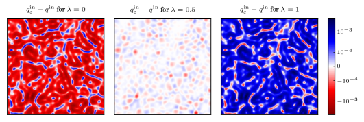
In Figure 1, we show the difference between the corresponding initial potential vorticity field $q^{\operatorname{in}}$ and the transformed potential vorticity fields $q_{\varepsilon}^{\operatorname{in}}$, for $\lambda=0,\tfrac{1}{2},1$ and an intermediate value of $\varepsilon$. Note that this difference is not measuring the quality of the initialization or the amount of imbalance, as $q^{\operatorname{in}}$ and $q_{\varepsilon}^{\operatorname{in}}$ live in different spaces. The figure just serves to illustrate that for $\lambda\neq\tfrac{1}{2}$, the transformation produces significantly different fields.

For $\lambda=0$ and $1$, and for $\varepsilon=2^{-5}$, the differences between the untransformed GLSG fields $q^{\operatorname{in}}$ and the corresponding rotating shallow water equation fields $q_{\varepsilon}^{\operatorname{in}}$ are about $0.06\%$, whereas the case $\lambda=\tfrac{1}{2}$ produces differences which are $40$ times less. This is expected as for $\lambda=\tfrac{1}{2}$, by construction, the difference between $\operatorname{T}[q^{\operatorname{in}}]$ and $q^{\operatorname{in}}$ is ${\mathcal{O}}(\varepsilon^{2})$.

We remark that for $\lambda=0$ and $1$ the differences between transformed and untransformed initial height fields are about $0.3\%$, i.e. almost one order of magnitude larger than the differences in the potential vorticity fields.

5 Results

5.1 Flow evolution

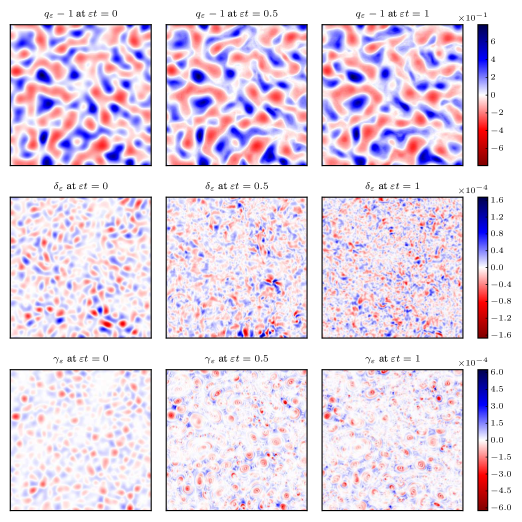
Figure 2 demonstrates how the shallow water flow fields, initialized by the balancing procedure described in Section 3.4, evolve on a time scale of ${\mathcal{O}}(1/\varepsilon)$. Shown are the potential vorticity anomaly $q_{\varepsilon}-1$, divergence $\delta_{\varepsilon}$ and ageostrophic vorticity $\gamma_{\varepsilon}$ at the initial time $t=0$, an intermediate time $t=0.5/\varepsilon$, and the final time $t=1/\varepsilon$, for Rossby number $\varepsilon=2^{-5}$. Whereas the potential vorticity appears broadly similar at these two times, the divergence and ageostrophic vorticity exhibit major changes. Only a small part of these changes is due to imbalanced motions, as seen below.

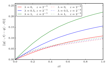
We now establish that the Eulerian evolutionary time scale is, as theorized in Appendix B, of ${\mathcal{O}}(1/\varepsilon)$, independent of $\lambda$. We do so by monitoring the change of the Eulerian potential vorticity up to time $t=\varepsilon^{-1}$. The result is shown in Figure 3. In particular, the final time difference $\left\lVert q(\,\cdot\,,\varepsilon^{-1})-q(\,\cdot\,,0)\right\rVert$ is approximately independent of the Rossby number $\varepsilon$, and approximately independent of $\lambda$. This justifies evolving the dynamics to time $t=\varepsilon^{-1}$ to assess the order of accuracy to which the GLSG balance models are able to approximate nearly balanced shallow water flows. The results of this analysis are presented below in Section 5.3.

Figure 3: Amount of flow evolution between $t=0$ and $t=\varepsilon^{-1}$ as measured by the quantity $\left\lVert q(\,\cdot\,,t)-q(\,\cdot\,,0)\right\rVert$, as a function of Rossby number $\varepsilon$, for $\lambda=0$, $\tfrac{1}{2}$, and $1$, as indicated.

5.2 Comparison between the shallow water and GLSG dynamics

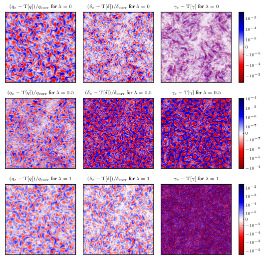
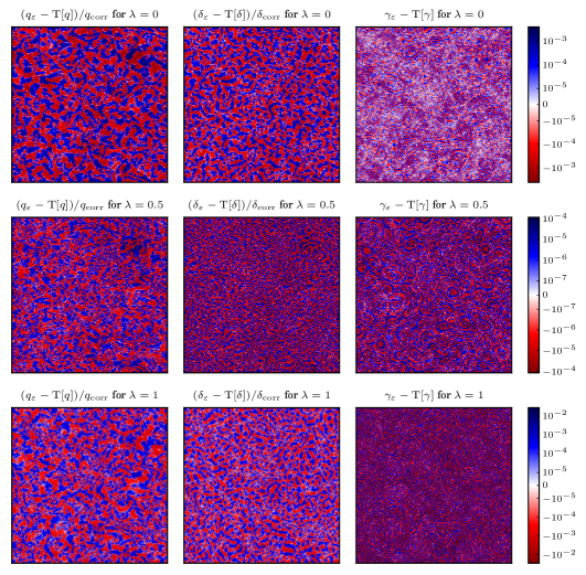
Before investigating the scaling behavior of the error (44) with $\varepsilon$, we examine the actual difference fields between the shallow water fields $q_{\varepsilon}$, $\delta_{\varepsilon}$, and $\gamma_{\varepsilon}$, and the corresponding transformed balance fields $\operatorname{T}[q]$, $\operatorname{T}[\delta]$, and $\operatorname{T}[\gamma]$ for $\lambda=0$, $\tfrac{1}{2}$, and $1$. Note, by construction, these difference fields are identically zero at $t=0$. From the earliest times, we see a clear distinction between the cases $\lambda=\tfrac{1}{2}$ and $\lambda\neq\tfrac{1}{2}$ — see Figures 4 and 5 for $t=0.1/\varepsilon$ and $t=1/\varepsilon$, respectively. The differences in potential vorticity are $60$ times smaller for $\lambda=\tfrac{1}{2}$ than for $\lambda=0$ or $1$. The differences in divergence are $15$ times smaller for $\lambda=\tfrac{1}{2}$ than for $\lambda=0$ or $1$. Both fields, however, show similar structures. The most remarkable differences between the cases $\lambda=\tfrac{1}{2}$ and $\lambda\neq\tfrac{1}{2}$ are seen in the ageostrophic vorticity. Here the differences are $8$ times larger for $\lambda=0$ and $250$ times larger for $\lambda=1$ when compared to $\lambda=\tfrac{1}{2}$. Moreover, whereas the structure of the difference field resembles the actual ageostrophic vorticity field in the case $\lambda=\tfrac{1}{2}$ (cf. Figure 2), the streak-like concentration of $\gamma$ in the cases $\lambda=0$ and $\lambda=1$ appears to be unphysical. When $\lambda=\tfrac{1}{2}$, we see ageostrophic wave-train like structures not only in the potential vorticity difference field, but also in the divergence and ageostrophic vorticity. These structures tend to be most prominent in regions of significant potential vorticity anomalies.

Figure 4: Early time differences ($\varepsilon t=0.1$) between the shallow water fields $q_{\varepsilon}$, $\delta_{\varepsilon}$, and $\gamma_{\varepsilon}$, and the corresponding transformed balance model fields for $\varepsilon=2^{-5}$ and for three different values of $\lambda$. The correction factors $q_{\operatorname{corr}}$ and $\delta_{\operatorname{corr}}$ are chosen so that the differences in $q$, $\delta$, and $\gamma$ have exactly the same range of values for the late-time ($\varepsilon t=1$) frames in the most accurate case $\lambda=\tfrac{1}{2}$.

Figure 5: Late time relative differences (at $\varepsilon t=1$) of the difference between shallow water fields and corresponding transformed balance model fields. All other parameters and normalizing values are the same as in Figure 4. Note that the color scales are the same as for the corresponding rows in Figure 4 so that the growth in color saturation gives an impression of the growth in the error as time progresses.

5.3 Asymptotic scaling with Rossby number

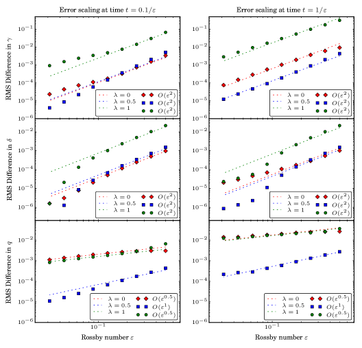
We next consider how the errors, as measured by the r.m.s. differences $\mathcal{E}_{\gamma}$, $\mathcal{E}_{\delta}$, and $\mathcal{E}_{q}$, defined in (44), scale with Rossby number $\varepsilon$ for various choices of $\lambda$. These results are presented in Figure 6, at early time $t=0.1/\varepsilon$ on the left and at the final time $t=1/\varepsilon$ on the right. First of all, the error grows in time, as expected, but preserves its Rossby number scaling. Both $\gamma$ and $\delta$ exhibit an ${\mathcal{O}}(\varepsilon^{2})$ scaling overall; the departures at small $\varepsilon$ are largely numerical artifacts (damping), as has been verified in double-resolution simulations. Most significantly, the errors in potential vorticity (bottom panels) exhibit a shallower scaling, and one which clearly distinguishes $\lambda=\frac{1}{2}$ from $\lambda\neq\frac{1}{2}$. Not only are the errors for $\lambda\neq\frac{1}{2}$ significantly larger than for $\lambda=\frac{1}{2}$, their scaling with $\varepsilon$ is also significantly shallower. This is attributed to the poor representation of the ageostrophic dynamics for $\lambda\neq\frac{1}{2}$, already seen in Figures 4 and 5.

5.4 Dependence on $\lambda$

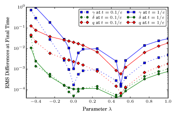
The strikingly different behavior for different values of $\lambda$ is seen more explicitly in Figure 7, now showing the dependence of the r.m.s. differences on $\lambda$ for a fixed Rossby number $\varepsilon=2^{-3}$. Dashed lines show early time results, while the solid lines show the final time. There is a dip in all three error measures at $\lambda=\frac{1}{2}$, but it is most pronounced for $\mathcal{E}_{\gamma}$ (blue curves). Interestingly, a second weaker dip occurs at $\lambda=0$, though not for $\mathcal{E}_{q}$. When $\lambda=0$ the regularity of the velocity field is expected to be greater than that of the height field, since the high derivative terms on the right-hand side of (23) are absent. This evidently results in much smaller errors, principally in $\mathcal{E}_{\gamma}$, compared to nearby surrounding values of $\lambda$, but not as small as the errors found for $\lambda=\frac{1}{2}$. As $\lambda$ decreases further, the errors grow steeply and diverge as $\lambda\to-\frac{1}{2}$, where the balance model becomes mathematically ill-posed.

In summary, $\lambda=\frac{1}{2}$ has much weaker errors in all three measures than any other $\lambda$, even values close to $\lambda=\frac{1}{2}$. The exception is $\mathcal{E}_{\delta}$, which appears to be less sensitive to $\lambda$. This is consistent with the mathematical analysis in Section 3.3, specifically (35a), where no significant gain in regularity is seen for $\lambda=\frac{1}{2}$ (or for $\lambda=0$). Nonetheless, even for $\delta$, the choice $\lambda=\frac{1}{2}$ leads to nearly the smallest errors. Most importantly, errors in potential vorticity $q$ exhibit a single, pronounced minimum at the value $\lambda=\frac{1}{2}$. This implies that the balance model for $\lambda=\frac{1}{2}$, i.e. the $L_{1}$-model, offers the most accurate prediction of nearly balanced shallow water flow.

Figure 6: R.m.s. differences $\mathcal{E}_{\gamma}$ (top), $\mathcal{E}_{\delta}$ (middle), and $\mathcal{E}_{q}$ (bottom) as a function of Rossby number $\varepsilon$, for various $\lambda$ as indicated, with the early time results ($t=0.1/\varepsilon$) shown on the left, and the late time results ($t=1/\varepsilon$) shown on the right.

Figure 7: R.m.s. differences $\mathcal{E}_{\gamma}$ (blue), $\mathcal{E}_{\delta}$ (green), and $\mathcal{E}_{q}$ (red) as a function of $\lambda$, for fixed Rossby number $\varepsilon=2^{-3}$, at $t=0.1/\varepsilon$ (dashed lines) and $t=1/\varepsilon$ (solid lines).

5.5 Power spectra and regularity

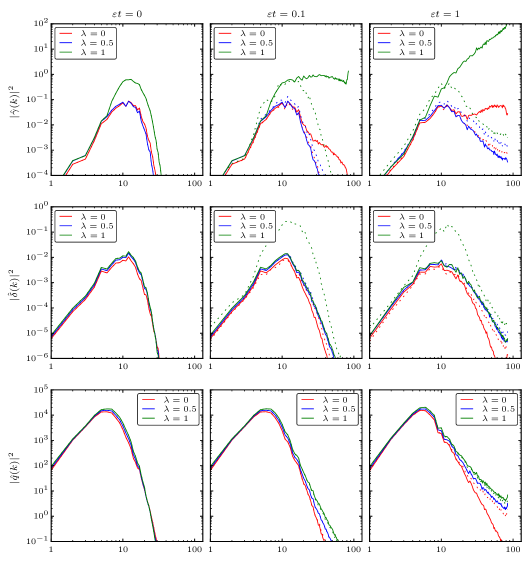
In Figure 8 we show power spectra for potential vorticity, divergence and ageostrophic vorticity, both on the GLSG balance model side and on the shallow water side. Whereas the spectra of potential vorticity and of divergence each exhibit closely similar forms for the different values of $\lambda$ and model dynamics, the ageostrophic vorticity spectra exhibit large differences from the earliest times. The ageostrophic vorticity spectra for $\lambda=0$ and $\lambda=1$ rapidly develop strong high-wavenumber contributions which dominate the spectra. This erroneous behavior corresponds to the intense frontal structures seen in the difference fields in Figures 4 and 5. By contrast, the ageostrophic vorticity spectrum for $\lambda=\tfrac{1}{2}$ exhibits a closely similar, decaying form on both the GLSG and shallow water sides at all times.

It is also noteworthy that, only for $\lambda=\tfrac{1}{2}$, the spectrum for $\operatorname{T}[q]$ is steeper than that of the corresponding $q_{\varepsilon}$. This is to be expected for a reliable balance model, as it allows for higher wavenumber contributions of inertia-gravity waves in the shallow water equations expressing the departure from balance.

Figure 8: Power density spectra for ageostrophic vorticity (top), divergence (middle), and potential vorticity (bottom), at times $t=0$ (left), $t=0.1/\varepsilon$ (middle), and $t=1/\varepsilon$ (right). Here $\varepsilon=2^{-3}$, and three different values of $\lambda$ are compared (see legend). Dashed lines are used for the shallow water fields $\gamma_{\varepsilon}$, $\delta_{\varepsilon}$, and $q_{\varepsilon}$, while solid lines are used for the corresponding transformed balance fields $\operatorname{T}[\gamma]$, $\operatorname{T}[\delta]$, and $\operatorname{T}[q]$.

Figure 9: Power density spectra for the balance model $q$, $h$, and ${\boldsymbol{u}}$ for $\varepsilon=2^{-3}$, and for different values of $\lambda$ at time $\varepsilon t=1$.

Figure 10: Power density spectra for each of the terms on the right hand side of the $\gamma$-equation (35b), upper panel, and of the $\delta$-equation (35a), lower panel, corresponding to the case shown in Figure 9.

We now look at the terms affecting the regularity of the solutions to the GLSG balance relation in more detail. To help interpret the results properly, we note that when the Fourier coefficients $a_{\boldsymbol{k}}$ of a two-dimensional field $a$ decay like $\lvert{\boldsymbol{k}}\rvert^{-p}\equiv k^{-p}$, then the power spectrum decays like $k^{1-2p}$.

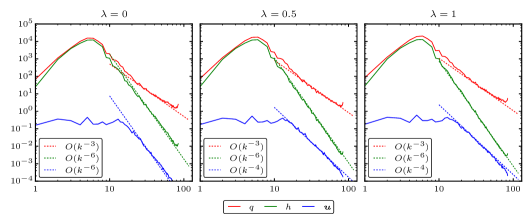
Figure 9 shows the power spectra of $q$, $h$, and ${\boldsymbol{u}}$. The power spectrum of $h$ decays robustly like $k^{-6}$ independent of $\lambda$, corresponding to $h_{\boldsymbol{k}}\sim k^{-7/2}$. The regularity of ${\boldsymbol{u}}$ is best when $\lambda=0$. However, since for $\lambda=0$ the balance relation (23) implies that ${\boldsymbol{u}}$ is one derivative smoother than $h$, we would expect a decaying velocity power spectrum proportional to $k^{-8}$. The observed reduced spectral decay is presumably due to nonlinear effects. The lack of regularity for $\lambda\neq\tfrac{1}{2}$ noted above predominantly affects the ageostrophic part of the flow, whereas $q$, $h$, and ${\boldsymbol{u}}$ are dominated by the geostrophic part of the flow which masks the deterioration of the smaller ageostrophic part.

Diagnosing the balance relation in ageostrophic variables, however, offers an explanation for the observed deterioration when $\lambda\neq\tfrac{1}{2}$. This is done in Figure 10, which displays the final time power density spectra for each of the terms on the right hand side of the $\gamma$-equation (35b) and of the $\delta$-equation (35a). The term with the highest number of derivatives on the right hand side of the equation for $\gamma$, namely $(\tfrac{1}{2}-\lambda)\,h\,\Delta^{2}h$, gives rise to a spectrum increasing as $k^{2}$ for both $\lambda=0$ and $\lambda=1$. As a result, even though the elliptic operator on the left hand side gains some regularity, the spectrum of $\gamma$ shows no decrease when $\lambda=0$, and only a slight decrease when $\lambda=1$. This saturation at high wavenumbers is unphysical. When $\lambda=\tfrac{1}{2}$, the dominant term on the right hand side of (35b) has a power spectrum decaying like $k^{-2}$ and the elliptic inversion gains the expected two derivatives, so that the power spectrum of $\gamma$ decays like $k^{-6}$.

The equation for $\delta$, (35a), does not have any $\lambda$-dependent irregular terms on its right hand side and is therefore much less sensitive to $\lambda$. However, it is clearly evident that when $\lambda\neq\tfrac{1}{2}$, the poor spectral decay of $\gamma$ contaminates some of the normally sub-dominant terms on the right hand side to reduce the spectral decay of $\delta$. This is particularly evident when $\lambda=0$.

For $\lambda=\tfrac{1}{2}$ in particular, the right hand side of (35b) is dominated by two derivatives on $h$. Since $h_{\boldsymbol{k}}\sim k^{-7/2}$ as observed in Figure 9, then the right hand side of (35b) should exhibit a Fourier decay like $k^{-3/2}$, resulting in $\gamma_{\boldsymbol{k}}\sim\lvert k\rvert^{-7/2}$. The corresponding dominant term on the right hand side of (35a) for $\delta$, namely $\boldsymbol{\nabla}h\boldsymbol{\cdot}\boldsymbol{\nabla}^{\bot}\Delta h$, contains three derivatives on $h$, and thus is expected to have a flat power spectrum. Yet, the observed power spectrum for this term decays like $k^{-1}$, corresponding to a $k^{-1}$ decay of its Fourier coefficients, and therefore $\delta_{\boldsymbol{k}}\sim k^{-3}$ after inversion of the elliptic operator. Its spectrum is steeper than the spectrum of the term $\boldsymbol{\nabla}h\boldsymbol{\cdot}\boldsymbol{\nabla}\Delta h$ on the right hand side of (35b), which suggests that there is some cancellation within the nonlinear contributions that is not currently understood.

We finally remark that the absolute slopes see in Figures 9 and 10 do not represent a late-time steady state characterized by sharp potential vorticity gradients. At this stage of the evolution, they are still in the process of steepening. The relative slopes, however, are robust.

6 Discussion and outlook

We have examined a family of variational balance models relevant to the small Rossby number, semi-geostrophic regime of the rotating shallow water equations. This family, originally derived by Oliver (2006), is spanned by a parameter $\lambda$ and includes the $L_{1}$-model introduced by Salmon (1983) as a special case ($\lambda=\frac{1}{2}$). To test the quality of these models, we have compared them against initially balanced shallow water numerical simulations for a wide range of Rossby numbers $\varepsilon$. This has revealed that the $L_{1}$-model, obtained for the specific parameter value $\lambda=\frac{1}{2}$, strongly outperforms all other members of the family. That is, the $L_{1}$-model gives the closest comparison with the full shallow water dynamics over an ${\mathcal{O}}(\varepsilon^{-1})$ time scale. Given that all models are formally of the same asymptotic order, and that the case $\lambda=0$ seems preferable from the regularity theory point of view, this result was initially unexpected. However, we have been able to explain the superior performance of the $L_{1}$-model by rewriting the balance model in terms of ageostrophic quantities, where the ageostrophic vorticity is most regular when $\lambda=\tfrac{1}{2}$. Our numerical diagnostics confirm that this interpretation is consistent with the actual model behavior. In particular, the ageostrophic vorticity for $\lambda=\frac{1}{2}$ exhibits a steeply decaying spectrum, in close agreement with the full shallow water dynamics. On the other hand, the ageostrophic vorticity for $\lambda\neq\frac{1}{2}$ exhibits a flat or rising spectrum. This unphysical feature spoils the comparison with the full shallow water dynamics. This finding underscores the critical importance of understanding, and ensuring, the mathematical regularity of any balance model. We further remark that the observed superior performance of the $L_{1}$ model is consistent with the study of Allen et al. (2002) who find that the stratified version of the $L_{1}$ model and its next order correction outperform a selection of other balance models in a simple direct numerical comparison.

Over longer time scales, randomly initialised shallow-water flows generically exhibit a direct enstrophy (potential vorticity variance) cascade to small scales, leading to sharp fronts and fine scale filamentary debris, particularly in potential vorticity. As a result, predictability is first lost at small scales then progressively at larger scales due to nonlinear scale interactions. This makes any direct comparison with a balance model difficult, though it may still be meaningful to compare statistical properties. The methods used in the present paper were designed to address how different balance models compare to the full shallow water model before any significant small-scale structure develops. i.e. while the flow is still predictable at all scales considered. Different methods, better suited to preserving conservation laws (to the extent possible), would be needed to study both the balanced and shallow-water dynamics at longer times, e.g. as in Mohebalhojeh & Dritschel (2001).

There are several new ideas to pursue emerging from the work presented here. We have focused above on a particular form of the initial conditions. It would be interesting to see how the balanced GLSG models perform in flows starting from a few, well-separated vortical structures, and where the largest velocity gradients are concentrated in thin jets of width comparable to the Rossby radius of deformation $L_{D}$. Notably, the balance relation (23) exhibits consistent scaling in this scenario. The concentration of fluid flow in jets of width $L_{D}$ implies $u\sim fL_{D}\sim\sqrt{\varepsilon}$ and $\boldsymbol{\nabla}\sim 1/\sqrt{\varepsilon}$. Since ${\boldsymbol{u}}\approx\boldsymbol{\nabla}^{\bot}h$ we have $h\sim\varepsilon$. Assuming that the jets are characterized (in the worst case) by jumps in potential vorticity, which have at worst a spectral scaling $q_{\boldsymbol{k}}\sim k^{-1}$, we have ${\boldsymbol{u}}_{\boldsymbol{k}}\sim k^{-2}$ and $h_{\boldsymbol{k}}\sim k^{-3}$. The balance relation (23) is invariant under this scaling.

In future work, we plan to compare the GLSG balance models studied here with other models used in the literature. In particular, it will be instructive to see how the geometric GLSG equations compare with more traditional balance models obtained by performing the asymptotics directly to the equations of motion. Examples include the $\delta$-$\gamma$ hierarchy of balance models introduced by Mohebalhojeh & Dritschel (2001) and the semi-geostrophic equations which are presumed valid specifically in the frontal regime (Cullen, 2008).

Of particular interest is the behavior of the $L_{1}$-model, and possibly other models from the GLSG family, in spherical geometry. At the formal level, the variational derivation of the models should translate naturally to spherical geometry. However, it is less clear whether the resulting balance models remain mathematically well posed and can be simulated in a robust way as the Coriolis parameter degenerates at the equator. Previous work by Oliver & Vasylkevych (2013) suggests that robust solvability at mid-latitudes may only be possible if the transformation vector field ${\boldsymbol{v}}$ is nontrivial at leading order, i.e., if one moves away from Salmon’s $L_{1}$ model. This work would need to be revisited in the light of rewriting the balance relation in terms of ageostrophic quantities. An independent issue is the study of degeneracy near the equator. We plan to address these questions in future work.

Although we have not considered the problem of quantifying the amount of imbalance (or gravity wave activity) associated with the initialization procedure in this work, our framework permits us to do so. By employing the dynamic global iteration rebalancing procedure, described in Appendix C, we can compute at each time step the difference between the time-evolved shallow water fields and their rebalanced forms. If the balance model used to rebalance the fields is accurate, the difference would be dominated by gravity waves, at least for small Rossby numbers. This could be tested by looking at the frequency spectra of those rebalanced differences. This is planned for future work.

Appendix A Derivation of the balance model Euler–Lagrange equation

Let us now compute the variation of each of the four terms appearing in $L_{\operatorname{bal}}$ in (22). First, up to perfect time derivatives which are null-Lagrangians as they do not contribute to the variation of the action integral,

$$\delta\int {\boldsymbol{R}}\circ{\boldsymbol{\eta}}\boldsymbol{\cdot}\dot{\boldsymbol{\eta}}\,{\mathrm{d}}{\boldsymbol{a}}=\int\bigl{[}\boldsymbol{\nabla}{\boldsymbol{R}}\circ{\boldsymbol{\eta}}\,\delta{\boldsymbol{\eta}}\boldsymbol{\cdot}\dot{\boldsymbol{\eta}}+{\boldsymbol{R}}\circ{\boldsymbol{\eta}}\boldsymbol{\cdot}\delta\dot{\boldsymbol{\eta}}\bigr{]}\,{\mathrm{d}}{\boldsymbol{a}}$$

$$=\int\bigl{[}\boldsymbol{\nabla}{\boldsymbol{R}}^{T}\circ{\boldsymbol{\eta}}\,\dot{\boldsymbol{\eta}}\boldsymbol{\cdot}\delta{\boldsymbol{\eta}}-\boldsymbol{\nabla}{\boldsymbol{R}}\circ{\boldsymbol{\eta}}\,\dot{\boldsymbol{\eta}}\boldsymbol{\cdot}\delta{\boldsymbol{\eta}}\bigr{]}\,{\mathrm{d}}{\boldsymbol{a}}=-\int h\,{\boldsymbol{w}}\boldsymbol{\cdot}{\boldsymbol{u}}^{\bot}\,{\mathrm{d}}{\boldsymbol{x}}\,.$$ (45)

The last identity holds as $\boldsymbol{\nabla}^{\bot}\boldsymbol{\cdot}{\boldsymbol{R}}=1$, which implies that $\boldsymbol{\nabla}{\boldsymbol{R}}-\boldsymbol{\nabla}{\boldsymbol{R}}^{T}=\mathsf{J}$, the standard symplectic matrix.

Second,

$$\delta\int \boldsymbol{\nabla}^{\bot}h\circ{\boldsymbol{\eta}}\boldsymbol{\cdot}\dot{\boldsymbol{\eta}}\,{\mathrm{d}}{\boldsymbol{a}}=\int\bigl{[}\boldsymbol{\nabla}^{\bot}\delta h\circ{\boldsymbol{\eta}}\boldsymbol{\cdot}\dot{\boldsymbol{\eta}}+\boldsymbol{\nabla}\boldsymbol{\nabla}^{\bot}h\circ{\boldsymbol{\eta}}\,\delta{\boldsymbol{\eta}}\boldsymbol{\cdot}\dot{\boldsymbol{\eta}}+\boldsymbol{\nabla}^{\bot}h\circ{\boldsymbol{\eta}}\boldsymbol{\cdot}\delta\dot{\boldsymbol{\eta}}\bigr{]}\,{\mathrm{d}}{\boldsymbol{a}}$$

$$=\int\bigl{[}\boldsymbol{\nabla}^{\bot}\delta h\circ{\boldsymbol{\eta}}\boldsymbol{\cdot}\dot{\boldsymbol{\eta}}+\boldsymbol{\nabla}^{\bot}\boldsymbol{\nabla}h\circ{\boldsymbol{\eta}}\,\dot{\boldsymbol{\eta}}\boldsymbol{\cdot}\delta{\boldsymbol{\eta}}-\boldsymbol{\nabla}^{\bot}\dot{h}\circ{\boldsymbol{\eta}}\boldsymbol{\cdot}\delta{\boldsymbol{\eta}}-\boldsymbol{\nabla}\boldsymbol{\nabla}^{\bot}h\circ{\boldsymbol{\eta}}\,\dot{\boldsymbol{\eta}}\boldsymbol{\cdot}\delta{\boldsymbol{\eta}}\bigr{]}\,{\mathrm{d}}{\boldsymbol{a}}$$

$$=\int h\,\bigl{[}-\boldsymbol{\nabla}^{\bot}\boldsymbol{\nabla}\boldsymbol{\cdot}(h{\boldsymbol{w}})\boldsymbol{\cdot}{\boldsymbol{u}}+\boldsymbol{\nabla}^{\bot}\boldsymbol{\nabla}h\,{\boldsymbol{u}}\boldsymbol{\cdot}{\boldsymbol{w}}+\boldsymbol{\nabla}^{\bot}\boldsymbol{\nabla}\boldsymbol{\cdot}(h{\boldsymbol{u}})\boldsymbol{\cdot}{\boldsymbol{w}}-\boldsymbol{\nabla}\boldsymbol{\nabla}^{\bot}h\,{\boldsymbol{u}}\boldsymbol{\cdot}{\boldsymbol{w}}\bigr{]}\,{\mathrm{d}}{\boldsymbol{x}}$$

$$=\int h\,\bigl{[}-\boldsymbol{\nabla}\boldsymbol{\nabla}^{\bot}\boldsymbol{\cdot}(h{\boldsymbol{u}})\boldsymbol{\cdot}{\boldsymbol{w}}+\boldsymbol{\nabla}^{\bot}\boldsymbol{\nabla}h\,{\boldsymbol{u}}\boldsymbol{\cdot}{\boldsymbol{w}}+\boldsymbol{\nabla}^{\bot}\boldsymbol{\nabla}\boldsymbol{\cdot}(h{\boldsymbol{u}})\boldsymbol{\cdot}{\boldsymbol{w}}-\boldsymbol{\nabla}\boldsymbol{\nabla}^{\bot}h\,{\boldsymbol{u}}\boldsymbol{\cdot}{\boldsymbol{w}}\bigr{]}\,{\mathrm{d}}{\boldsymbol{x}}$$

$$=\int h\,\bigl{[}h\,\Delta{\boldsymbol{u}}^{\bot}+2\,\boldsymbol{\nabla}h\boldsymbol{\cdot}\boldsymbol{\nabla}{\boldsymbol{u}}^{\bot}\bigr{]}\boldsymbol{\cdot}{\boldsymbol{w}}\,{\mathrm{d}}{\boldsymbol{x}}\,,$$ (46)

again up to perfect time derivatives, which we have subtracted in the second equality (equivalent to integration by parts with respect to time under the action integral). In the third equality, we have changed to Eulerian variables and have made use of the momentum and continuity equations. The fourth equality results from an integration by parts, and the last equality is straightforward vector algebra.

Third,

$$\frac{1}{2}\,\delta\int h^{2}\,{\mathrm{d}}{\boldsymbol{x}}=\int h\,\delta h\,{\mathrm{d}}{\boldsymbol{x}}=-\int h\,\boldsymbol{\nabla}\boldsymbol{\cdot}(h{\boldsymbol{w}})\,{\mathrm{d}}{\boldsymbol{x}}=\int h\,{\boldsymbol{w}}\boldsymbol{\cdot}\boldsymbol{\nabla}h\,{\mathrm{d}}{\boldsymbol{x}}\,.$$ (47)

Fourth,

$$\delta\int h\,\lvert\boldsymbol{\nabla}h\rvert^{2}\,{\mathrm{d}}{\boldsymbol{x}} =\int\bigl{[}\delta h\,\lvert\boldsymbol{\nabla}h\rvert^{2}+2\,h\,\boldsymbol{\nabla}h\boldsymbol{\cdot}\boldsymbol{\nabla}\delta h\bigr{]}\,{\mathrm{d}}{\boldsymbol{x}}$$

$$=-\int\bigl{[}\boldsymbol{\nabla}\boldsymbol{\cdot}(h{\boldsymbol{w}})\,\lvert\boldsymbol{\nabla}h\rvert^{2}+2\,h\,\boldsymbol{\nabla}h\boldsymbol{\cdot}\boldsymbol{\nabla}\boldsymbol{\nabla}\boldsymbol{\cdot}(h{\boldsymbol{w}})\bigr{]}\,{\mathrm{d}}{\boldsymbol{x}}$$

$$=\int h\,{\boldsymbol{w}}\boldsymbol{\cdot}\bigl{[}\boldsymbol{\nabla}\lvert\boldsymbol{\nabla}h\rvert^{2}-2\,\boldsymbol{\nabla}\boldsymbol{\nabla}\boldsymbol{\cdot}(h\boldsymbol{\nabla}h)\bigr{]}\,{\mathrm{d}}{\boldsymbol{x}}$$

$$=-\int h\,{\boldsymbol{w}}\boldsymbol{\cdot}\boldsymbol{\nabla}\bigl{[}2\,h\,\Delta h+\lvert\boldsymbol{\nabla}h\rvert^{2}\bigr{]}\,{\mathrm{d}}{\boldsymbol{x}}\,.$$ (48)

Plugging the results from (45) to (48) back into the variation of the action associated with (22), we find that stationary points of this action imply the Euler–Lagrange equation (23).

Appendix B Time scale of the Eulerian dynamics

To leading order, the motion induced by a velocity field computed from (23) is geostrophic with an ${\mathcal{O}}(1)$ velocity. Thus, fluid parcels travel a unit distance over times of ${\mathcal{O}}(1)$. The question is: on what time scale do Eulerian quantities change? To answer this, we conduct a kinematic analysis, in which we assume that ${\boldsymbol{u}}$ is constrained by the balance relation (23), and then estimate the magnitude of $\partial_{t}h$ and $\partial_{t}h_{\varepsilon}$.

First, we rearrange the balance relation (23) so that

$${\boldsymbol{u}}^{\bot}+\,\boldsymbol{\nabla}h=\varepsilon\,\bigl{[}(\lambda+\frac{1}{2})\,(h\,\Delta{\boldsymbol{u}}^{\bot}+2\boldsymbol{\nabla}h\boldsymbol{\cdot}\boldsymbol{\nabla}{\boldsymbol{u}}^{\bot})+\lambda\,\boldsymbol{\nabla}(2\,h\,\Delta h+\lvert\boldsymbol{\nabla}h\rvert^{2})\bigr{]}\,.$$ (49)

Re-insertion of leading-order geostrophic balance into (49) gives ${\boldsymbol{u}}=\boldsymbol{\nabla}^{\bot}h-\varepsilon\,{\boldsymbol{w}}^{\bot}+{\mathcal{O}}(\varepsilon^{2})$ with

$${\boldsymbol{w}}=(\lambda-\frac{1}{2})\,h\,\Delta\boldsymbol{\nabla}h-\boldsymbol{\nabla}h\boldsymbol{\cdot}\boldsymbol{\nabla}\boldsymbol{\nabla}h+2\lambda\,\boldsymbol{\nabla}h\,\Delta h\,.$$ (50)

Inserting ${\boldsymbol{u}}=\boldsymbol{\nabla}^{\bot}h-\varepsilon\,{\boldsymbol{w}}^{\bot}+{\mathcal{O}}(\varepsilon^{2})$ into the transformation (21), we obtain

$${\boldsymbol{v}}=(\lambda-\frac{1}{2})\,\boldsymbol{\nabla}h+\tfrac{1}{2}\,\varepsilon\,{\boldsymbol{w}}+{\mathcal{O}}(\varepsilon^{2})\,.$$ (51)

Similarly, inserting (50) into the continuity equation (24) gives

$$\dot{h} =-\boldsymbol{\nabla}\boldsymbol{\cdot}(h{\boldsymbol{u}})=\varepsilon\,\boldsymbol{\nabla}\boldsymbol{\cdot}(h{\boldsymbol{w}}^{\bot})+{\mathcal{O}}(\varepsilon^{2})$$

$$=\varepsilon\,\bigl{[}h\,\boldsymbol{\nabla}^{\bot}h\boldsymbol{\cdot}\boldsymbol{\nabla}\Delta h+\boldsymbol{\nabla}^{\bot}h\boldsymbol{\cdot}\boldsymbol{\nabla}\boldsymbol{\nabla}h\,\boldsymbol{\nabla}h\bigr{]}+{\mathcal{O}}(\varepsilon^{2})\,.$$ (52)

This shows that the time scale of Eulerian evolution in balance model coordinates is ${\mathcal{O}}(1/\varepsilon)$ and is, in particular, independent of $\lambda$ at this order. Moreover, we see that the time derivative of the transformation vector field vanishes to $\mathcal{O}(\varepsilon)$:

$$\dot{\boldsymbol{v}}=(\lambda-\frac{1}{2})\,\boldsymbol{\nabla}\dot{h}+{\mathcal{O}}(\varepsilon)={\mathcal{O}}(\varepsilon)\,.$$ (53)

A similar computation can be performed after transforming to the shallow water side. Using the diagnostic expressions for $h^{\prime}$ and ${\boldsymbol{u}}^{\prime}$, equations (17) and (18), respectively, we compute

$$\partial_{t}h_{\varepsilon} =-\boldsymbol{\nabla}\boldsymbol{\cdot}(h_{\varepsilon}{\boldsymbol{u}}_{\varepsilon})=-\boldsymbol{\nabla}\boldsymbol{\cdot}(h{\boldsymbol{u}})-\varepsilon\,\boldsymbol{\nabla}\boldsymbol{\cdot}(h^{\prime}{\boldsymbol{u}}+h{\boldsymbol{u}}^{\prime})+\mathcal{O}(\varepsilon^{2})$$

$$=-\boldsymbol{\nabla}\boldsymbol{\cdot}(h\boldsymbol{\nabla}^{\bot}h-\varepsilon\,h\,{\boldsymbol{w}}^{\bot})$$

$$\quad+\varepsilon\,(\lambda-\frac{1}{2})\,\boldsymbol{\nabla}\boldsymbol{\cdot}\bigl{(}\boldsymbol{\nabla}\boldsymbol{\cdot}(h\boldsymbol{\nabla}h)\,\boldsymbol{\nabla}^{\bot}h+h\,(\boldsymbol{\nabla}^{\bot}\boldsymbol{\nabla}^{\bot}h-\boldsymbol{\nabla}\boldsymbol{\nabla}h)\,\boldsymbol{\nabla}^{\bot}h\bigr{)}+\mathcal{O}(\varepsilon^{2})$$

$$=\tfrac{1}{4}\,\varepsilon\,\bigl{(}\boldsymbol{\nabla}^{\bot}h\boldsymbol{\cdot}\boldsymbol{\nabla}\Delta h^{2}-\boldsymbol{\nabla}^{\bot}\Delta h\boldsymbol{\cdot}\boldsymbol{\nabla}h^{2}\bigr{)}+\mathcal{O}(\varepsilon^{2})\,.$$ (54)

Thus, we obtain the same conclusion in shallow water coordinates as expected by consistency of the asymptotic derivation. In particular, the leading ${\mathcal{O}}(\varepsilon)$-term is independent of $\lambda$.

Appendix C The inverse transformation

In our setting, the transformation from balance model coordinates to physical coordinates is explicit and has been detailed in Section 3.4. However, it is also possible to invert the transformation in the following sense: given a shallow water potential vorticity $q_{\varepsilon}$ in physical coordinates, we seek a corresponding height field $h_{\varepsilon}$ and velocity field ${\boldsymbol{u}}_{\varepsilon}$, also in physical coordinates (or, equivalently, the divergence $\delta_{\varepsilon}$, ageostrophic vorticity $\gamma_{\varepsilon}$, and velocity mean $\bar{\boldsymbol{u}}_{\varepsilon}$) which, on the one hand, are consistent with the definition of the shallow water potential vorticity,

$$q_{\varepsilon}=\frac{1+\varepsilon\,\boldsymbol{\nabla}^{\bot}\boldsymbol{\cdot}{\boldsymbol{u}}_{\varepsilon}}{h_{\varepsilon}}\,,$$ (55)

and, on the other hand, are consistent with the balance relation (23) in transformed variables under the transformation (36). This can be achieved as follows.

We start by decomposing $q_{\varepsilon}=\bar{q}_{\varepsilon}+\hat{q}_{\varepsilon}$, where $\bar{q}_{\varepsilon}$ denotes the mean value of $q_{\varepsilon}$ and $\hat{q}_{\varepsilon}$ denotes the deviation from the mean, with corresponding notation for the other field variables. The expression for potential vorticity (55) can then be written in the form

$$(\bar{q}_{\varepsilon}-\varepsilon\Delta)\hat{h}_{\varepsilon}=1-\bar{q}_{\varepsilon}-\hat{q}_{\varepsilon}\,h_{\varepsilon}+\varepsilon\,\gamma_{\varepsilon}\,,$$ (56)

where we have used the definition of ageostrophic vorticity $\gamma_{\varepsilon}=\boldsymbol{\nabla}^{\bot}\boldsymbol{\cdot}{\boldsymbol{u}}_{\varepsilon}-\Delta h_{\varepsilon}$, as well as the fact that the mean height $\bar{h}_{\varepsilon}=1$. Equation (56) can be solved by iteration provided $\hat{q}_{\varepsilon}$ is sufficiently small. Next, to determine consistent balanced GLSG fields, we interpret the transformation of potential vorticity in the Lagrangian variables as

$$q_{\varepsilon}\circ{\boldsymbol{\eta}}_{\varepsilon}=q\,,$$ (57)

which leads to an advection equation with $\varepsilon$ playing the role of time, namely

$$q_{\varepsilon}^{\prime}+{\boldsymbol{v}}_{\varepsilon}\boldsymbol{\cdot}\boldsymbol{\nabla}q_{\varepsilon}=0\,,$$ (58)

where the prime denotes differentiation with respect to $\varepsilon$ and we integrate backwards from the given value of $\varepsilon$ to $\varepsilon=0$. Of course, we cannot have knowledge of the full transformation vector field ${\boldsymbol{v}}_{\varepsilon}$ as that would be akin to having an all-order balance model. For a first order model, it is consistent to approximate ${\boldsymbol{v}}_{\varepsilon}$ by ${\boldsymbol{v}}$ as given by (21). Thus, numerically, we are solving

$$q_{\varepsilon}^{\prime}+{\boldsymbol{v}}\boldsymbol{\cdot}\boldsymbol{\nabla}q_{\varepsilon}=0$$ (59)

as a backward advection equation with $\varepsilon$ as the artificial time variable.

The global iteration loop is then as follows. Given an initial potential vorticity field $q_{\varepsilon}$ on the shallow water side, initialize the iteration with ${\boldsymbol{u}}_{\varepsilon}^{\operatorname{ag}}=0$ (implying $\gamma_{\varepsilon}=0$ and $\delta_{\varepsilon}=0$). On the balance model side, initialize $q=q_{\varepsilon}$ and find initial $h$, ${\boldsymbol{u}}$, and ${\boldsymbol{v}}$ as in Steps 3–5 below.

1. Compute the corresponding height field $h_{\varepsilon}$ using (56).

2. Compute the potential vorticity $q$ on the balanced GLSG side by backwards advection in $\varepsilon$ to $\varepsilon=0$ using (59).

3. Compute the balanced GLSG height field $h$ via potential vorticity inversion (28).

4. Compute the corresponding GSLG velocity field ${\boldsymbol{u}}$ using the balance relation (23).

5. Compute ${\boldsymbol{v}}$ via (21).

6. Transform back to the shallow water side using (36) to compute $h_{\varepsilon}$ and ${\boldsymbol{u}}_{\varepsilon}$.

7. Update the ageostrophic velocity ${\boldsymbol{u}}_{\varepsilon}^{\operatorname{ag}}$, and go to Step 1.
   

Repeat until a fixed point is reached. Empirically, the procedure converges for small to moderate values for $\varepsilon$, but may fail to converge when $\varepsilon\approx 1$.

The procedure outlined above allows one to “rebalance” a given state of the shallow water evolution using any of the GLSG balance models. Given only the potential vorticity, all other fields can be reconstructed consistent with the balance relation, and the residual can be taken as a measure of imbalance.

References

- Allen & Holm (1996) Allen, J. S. & Holm, D. D. 1996 Extended-geostrophic Hamiltonian models for rotating shallow water motion. Phys. D 98 (2), 229–248.
- Allen et al. (2002) Allen, J. S., Holm, D. D. & Newberger, P. A. 2002 Toward an extended-geostrophic Euler–Poincaré model for mesoscale oceanographic flow. In Large-scale atmosphere–ocean dynamics (ed. J. Norbury & I. Roulstone), vol. 1, pp. 101–125. Cambridge University Press.
- Benamou & Brenier (1998) Benamou, J. D. & Brenier, Y. 1998 Weak existence for the semigeostrophic equations formulated as a coupled Monge–Ampère/transport problem. SIAM J. Appl. Math. 58 (5), 1450–1461.
- Bloom et al. (1996) Bloom, S. C., Takacs, L. L., Da Silva, A. M. & Ledvina, D. 1996 Data assimilation using incremental analysis updates. Mon. Weather Rev. 124, 1256–1271.
- Bretherton (1970) Bretherton, F. P. 1970 A note on Hamilton’s principle for perfect fluids. J. Fluid Mech. 44, 19–31.
- Çalık & Oliver (2013) Çalık, M. & Oliver, M. 2013 Weak solutions for generalized large-scale semigeostrophic equations. Commun. Pure Appl. Anal. 12 (2), 939–953.
- Çalık et al. (2013) Çalık, M., Oliver, M. & Vasylkevych, S. 2013 Global well-posedness for the generalized large-scale semigeostrophic equations. Arch. Ration. Mech. Anal. 207 (3), 969–990.
- Cullen (2008) Cullen, M. J. P. 2008 A comparison of numerical solutions to the eady frontogenesis problem. Quart. J. R. Meteorol. Soc. 134 (637), 2143–2155.
- Cullen & Purser (1984) Cullen, M. J. P. & Purser, R. J. 1984 An extended Lagrangian theory of semi-geostrophic frontogenesis. J. Atmos. Sci. 41 (9), 1477–1497.
- Eliassen (1948) Eliassen, A. 1948 The quasi-static equations of motion with pressure as independent variable. Geofys. Publ. 17, 1–44.
- Goldstein (1980) Goldstein, H. 1980 Classical Mechanics, 2nd edn. Addison-Wesley, Reading, MA.
- Gottwald (2014) Gottwald, G. A. 2014 Controlling balance in an ensemble Kalman filter. Nonlinear Proc. Geoph. 21, 417–426.
- Gottwald & Oliver (2014) Gottwald, G. A. & Oliver, M. 2014 Slow dynamics via degenerate variational asymptotics. Proc. R. Soc. Lond. Ser. A Math. Phys. Eng. Sci. 470 (2170), 20140460.
- Greybush et al. (2011) Greybush, S. J., Kalnay, E., Miyoshi, T., Ide, K. & Hunt, B. R. 2011 Balance and ensemble Kalman filter localization techniques. Mon. Weather Rev. 139 (2), 511–522.
- Hoskins (1975) Hoskins, B. J. 1975 The geostrophic momentum approximation and the semi-geostrophic equations. J. Atmos. Sci. 32 (2), 233–242.
- Kepert (2009) Kepert, J. D. 2009 Covariance localisation and balance in an ensemble Kalman filter. Quart. J. R. Meteorol. Soc. 135 (642), 1157–1176.
- Lynch (2006) Lynch, P. 2006 The Emergence of Numerical Weather Prediction: Richardson’s Dream. Cambridge University Press, Cambridge.
- McIntyre & Roulstone (2002) McIntyre, M. E. & Roulstone, I. 2002 Are there higher-accuracy analogues of semigeostrophic theory? In Large-scale atmosphere–ocean dynamics (ed. J. Norbury & I. Roulstone), vol. 2, pp. 301–364. Cambridge University Press.
- Mitchell et al. (2002) Mitchell, H. L., Houtekamer, P. L. & Pellerin, G. 2002 Ensemble size, balance, and model-error representation in an ensemble Kalman filter. Mon. Weather Rev. 130 (11), 2791–2808.
- Mohebalhojeh & Dritschel (2001) Mohebalhojeh, A. R. & Dritschel, D. G. 2001 Hierarchies of balance conditions for the -plane shallow-water equations. J. Atmos. Sci. 58 (16), 2411–2426.
- Mohebalhojeh & Dritschel (2004) Mohebalhojeh, A. R. & Dritschel, D. G. 2004 Contour-advective semi-Lagrangian algorithms for many-layer primitive equation models. Quart. J. R. Meteorol. Soc. 130, 347–364.
- Oliver (2006) Oliver, M. 2006 Variational asymptotics for rotating shallow water near geostrophy: a transformational approach. J. Fluid Mech. 551, 197–234.
- Oliver & Vasylkevych (2011) Oliver, M. & Vasylkevych, S. 2011 Hamiltonian formalism for models of rotating shallow water in semigeostrophic scaling. Discrete Contin. Dyn. Syst. 31 (3), 827–846.
- Oliver & Vasylkevych (2013) Oliver, M. & Vasylkevych, S. 2013 Generalized LSG models with spatially varying Coriolis parameter. Geophys. Astrophys. Fluid Dyn. 107, 259–276.
- Ourmiéres et al. (2006) Ourmiéres, Y., Brankart, J. M., Berline, L., Brasseur, P. & Verron, J. 2006 Incremental analysis update implementation into a sequential ocean data assimilation system. J. Atmos. Ocean. Tech. 23, 1729–1744.
- Richardson (1922) Richardson, L. F. 1922 Weather Prediction by Numerical Process. Cambridge University Press, Cambridge.
- Salmon (1983) Salmon, R. 1983 Practical use of Hamilton’s principle. J. Fluid Mech. 132, 431–444.
- Salmon (1985) Salmon, R. 1985 New equations for nearly geostrophic flow. J. Fluid Mech. 153, 461–477.
- Salmon (1998) Salmon, R. 1998 Lectures on Geophysical Fluid Dynamics. Oxford University Press, New York.
- Smith & Dritschel (2006) Smith, R. K. & Dritschel, D. G. 2006 Revisiting the Rossby–Haurwitz wave test case with contour advection. J. Comput. Phys. 217 (2), 473–484.
- Viúdez & Dritschel (2004) Viúdez, Á. & Dritschel, D. G. 2004 Optimal potential vorticity balance of geophysical flows. J. Fluid Mech. 521, 343–352.