Tidal Disruption of a White Dwarf by a Black Hole: The Diversity of Nucleosynthesis, Explosion Energy, and the Fate of Debris Streams

Abstract

We run a suite of hydrodynamics simulations of tidal disruption events (TDEs) of a white dwarf (WD) by a black hole (BH) with a wide range of WD/BH masses and orbital parameters. We implement nuclear reactions to study nucleosynthesis and its dynamical effect through release of nuclear energy. The released nuclear energy effectively increases the fraction of unbound ejecta. This effect is weaker for a heavy WD with 1.2 $\mathrm{M}_{\sun}$, because the specific orbital energy distribution of the debris is predominantly determined by the tidal force, rather than by the explosive reactions. The elemental yield of a TDE depends critically on the initial composition of a WD, while the BH mass and the orbital parameters also affect the total amount of synthesized elements. Tanikawa et al. (2017) find that simulations of WD–BH TDEs with low resolution suffer from spurious heating and inaccurate nuclear reaction results. In order to examine the validity of our calculations, we compare the amounts of the synthesized elements with the upper limits of them derived in a way where we can avoid uncertainties due to low resolution. The results are largely consistent, and thus support our findings. We find particular TDEs where early self-intersection of a WD occurs during the first pericentre passage, promoting formation of an accretion disc. We expect that relativistic jets and/or winds would form in these cases because accretion rates would be super-Eddington. The WD–BH TDEs result in a variety of events depending on the WD/BH mass and pericentre radius of the orbit.

1 Introduction

A star passing close to a black hole (BH) can be disrupted when the tidal force on the star exceeds its self-gravity. The disrupted star leaves debris bound to the BH, but also disperse unbound materials (e.g. Rees, 1988). The bound debris cause emission via various possible processes (for a review, see Stone et al. 2018). One way to produce the emission is collision of advanced and leading streams of bound debris (Shiokawa et al., 2015; Piran et al., 2015; Guillochon & Ramirez-Ruiz, 2015; Bonnerot et al., 2016; Hayasaki et al., 2016; Jiang et al., 2016). The second way is forming an accretion disc and a flare, where the radiation could be reprocessed by surrounding materials (Loeb & Ulmer, 1997; Bogdanović et al., 2004; Lodato & Rossi, 2011; Guillochon & Ramirez-Ruiz, 2013; Guillochon et al., 2014; Roth et al., 2016; Metzger & Stone, 2016; Roth & Kasen, 2017). Another way is forming relativistic jets that probably occur when the accretion rate exceeds the Eddington limit (Bloom et al. 2011; Levan et al. 2011; Burrows et al. 2011; Zauderer et al. 2011; Giannios & Metzger 2011; Cenko et al. 2012; Coughlin & Begelman 2014, 2015; Brown et al. 2015; Krolik et al. 2016; for a review, see Komossa 2015). In this tidal disruption event (TDE), we can consider various types of the disrupted star, such as a main-sequence-type star (MS), giant star, and planet (Kobayashi et al., 2004; Law-Smith et al., 2017).

TDEs of a white dwarf (WD) have unique features. First, the range of the BH mass is restricted to stellar and intermediate masses. A supermassive BH (SMBH) whose mass is larger than $10^{5}\,\mathrm{M}_{\sun}$ does not cause WD–BH TDEs because it swallows a WD before disrupting it tidally; there would be no observable signals except for gravitational waves (see Fig. 1; Luminet & Pichon 1989b; East 2014). In contrast, other types of stars, such as MSs and red giant stars, can be disrupted by an SMBH (Kobayashi et al., 2004; Law-Smith et al., 2017). Thus, WD–BH TDEs may provide interesting information on the existence and the properties of intermediate mass BHs (IMBHs).

The second feature is the explosive thermonuclear reactions of a WD. They are caused by strong compression owing to the tidal force perpendicular to the orbital plane. Such adiabatic compression leads to shock heating during pericentre passage, resulting in explosive thermonuclear reactions (Carter & Luminet, 1982; Bicknell & Gingold, 1983; Luminet & Pichon, 1989a; Rosswog et al., 2008, 2009; Haas et al., 2012; Sell et al., 2015; Tanikawa et al., 2017). If a substantial amount of radioactive nuclei, such as ⁵⁶Ni, is synthesized in unbound ejecta, their decay supplies nuclear energy into the ejecta, and the event may appear similar to Type I supernovae (SNe; MacLeod et al. 2016). Other signatures from the WD–BH TDEs, such as $\gamma$-ray bursts and gravitational waves, have also been discussed (Zalamea et al., 2010; Clausen & Eracleous, 2011; Haas et al., 2012; East, 2014; Cheng & Bogdanović, 2014; Shiokawa et al., 2015; Ioka et al., 2016).

There are a few key physical quantities that characterize WD–BH TDEs. One of them is the Schwarzschild radius of the BH $R_{S}=2GM_{\textrm{BH}}/c^{2}$, where $G$ is the gravitational constant, $M_{\textrm{BH}}$ is the BH mass, and $c$ is the speed of light. Another is the tidal radius $R_{t}\equiv R_{\textrm{WD}}\left(M_{\textrm{BH}}/M_{\textrm{WD}}\right)^{1/3}$, at which the tidal force exceeds the self-gravity. It is estimated to be

$$R_{t}\simeq 1.2\times 10^{10}\left(\frac{R_{\textrm{WD}}}{10^{9}\,\textrm{cm}}\right)\left(\frac{M_{\textrm{BH}}}{10^{3}\,\mathrm{M}_{\sun}}\right)^{1/3}\left(\frac{M_{\textrm{WD}}}{0.6\,\mathrm{M}_{\sun}}\right)^{-1/3}\textrm{cm},$$ (1)

where $R_{\textrm{WD}}$ is the WD radius, and $M_{\textrm{WD}}$ is the WD mass. We introduce the dimensionless penetration parameter $\beta\equiv R_{t}/R_{p}$, where $R_{p}$ is the pericentre radius of the orbit. A WD is tidally disrupted if $\beta\gtrsim 1$. Note that the criterion is slightly modified depending on the detailed structure of the WD (Luminet & Pichon, 1989b; Law-Smith et al., 2017; Mainetti et al., 2017). If we adopt general relativity (GR) and a parabolic orbit, there is a relationship between the pericentre radius $R_{p}$ and the specific angular momentum $j$ (see e.g. Shapiro & Teukolsky (1983)),

$$j=(R_{S}R_{p}c^{2})^{1/2}\left(1-\frac{R_{S}}{R_{p}}\right)^{-1/2}.$$ (2)

The boundary on whether a BH swallows a WD is expressed as $j=2R_{S}c$, $R_{p}=2\,R_{S}$, or

$$\beta\simeq 10\left(\frac{R_{\textrm{WD}}}{10^{9}\,\textrm{cm}}\right)\left(\frac{M_{\textrm{BH}}}{10^{3}\,\mathrm{M}_{\sun}}\right)^{-2/3}\left(\frac{M_{\textrm{WD}}}{0.6\,\mathrm{M}_{\sun}}\right)^{-1/3}.$$ (3)

If $j<2R_{S}c$, Equation 2 does not have a real solution for $R_{p}$. This corresponds to the situation where the WD would be directly captured by the BH, and then there would be no observable signals except for gravitational waves. The BH can also swallow a part of the WD in the first pericentre passage if $R_{p}\leq R_{\textrm{WD}}$, or

$$\beta\gtrsim 12\left(\frac{M_{\textrm{BH}}}{10^{3}\,\mathrm{M}_{\sun}}\right)^{1/3}\left(\frac{M_{\textrm{WD}}}{0.6\,\mathrm{M}_{\sun}}\right)^{-1/3}.$$ (4)

This situation is conventionally called, “the BH enters the WD" (Luminet & Pichon, 1989b). Note that in that case the BH is much smaller than the WD so that a tiny part of the WD is swallowed during the pericentre passage. As we will discuss in Section 3, an interesting class of TDEs occur in this case, where the WD is so strongly compressed that nuclear burning is triggered and the foregoing part of the disrupted debris hits the trailing part.

The parameter space where WD–BH TDEs occur is shown in Fig. 1. Thus, an SMBH with $M_{\textrm{BH}}\gtrsim 10^{5}\,\mathrm{M}_{\sun}$ cannot tidally disrupt a WD.

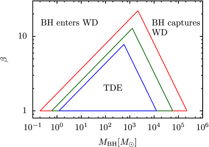
Figure 1: Parameter spaces where WD–BH TDEs occur. The red, green, and blue lines are for $M_{\textrm{WD}}=0.2$, 0.6, and 1.2 $\mathrm{M}_{\sun}$, respectively. The areas inside the triangles, respectively, correspond to the parameter spaces where TDEs occur. The original figure is given in Luminet & Pichon (1989b)

This feature of WD–BH TDEs is useful to investigate the properties of IMBHs. Once many WD–BH TDEs are observed, the number density and growing process of IMBHs could be constrained. So far, only a few candidates of WD–BH TDEs have been reported (Krolik & Piran, 2011; Shcherbakov et al., 2013; Jonker et al., 2013; Ioka et al., 2016; Bauer et al., 2017). Next-generation transient surveys, such as the Large Synoptic Survey Telescope, may detect a few tens of the events (MacLeod et al., 2016). It is expected that there would be a variety of observational signals originating from the diversity of the TDEs. Therefore, theoretical templates for various types of WD–BH TDEs are needed in order to detect them robustly by the future transient surveys.

If a WD passes very close to the BH, not only tidal disruption but also explosive thermonuclear burning is likely ignited by adiabatic compression and shock heating (Carter & Luminet, 1982; Bicknell & Gingold, 1983; Luminet & Pichon, 1989a; Rosswog et al., 2009; Tanikawa et al., 2017). Rosswog et al. (2009) use numerical simulations to study the WD–BH TDEs for 16 parameter sets. They conclude that the critical condition of the explosive thermonuclear reactions is $\beta\gtrsim 3$ for $1.2\,\mathrm{M}_{\sun}$ WDs. They also show that the release of nuclear energy increases the fraction of the unbound ejecta from about 50% to 65% of the initial mass of the WD, which affects the flare caused by the accretion of the bound debris on to the BH (MacLeod et al., 2014). MacLeod et al. (2016) study observational signatures and estimate a detection rate of the events using the results of Rosswog et al. (2009). They argue that the WD–BH TDEs with the explosive nuclear reactions would be the reminiscent of Type I SNe.

The 16 parameter sets in Rosswog et al. (2009) are not systematically chosen. They are not enough to comprehensively explore the parameter spaces shown in Fig. 1. The problem makes it difficult to reveal the variety of WD–BH TDEs and to determine detailed critical conditions on explosive nuclear reactions for various types of WDs.

In this paper, we explore the variety of WD–BH TDEs, focusing on nucleosynthesis and its effects on the debris of the disrupted WD. We perform a systematic and comprehensive parameter study for 184 parameter sets, changing $M_{\textrm{WD}}$, $M_{\textrm{BH}}$, and $\beta$. To this end, we use smoothed particle hydrodynamics (SPH) simulations coupled with the nuclear reactions of $\alpha$-chain networks among the 13 species from ⁴He to ⁵⁶Ni. Our numerical methods are largely based on the recent study of Tanikawa et al. (2017).

Tanikawa et al. (2017) show that the results of nucleosynthesis do not converge even with 25 millions SPH particles. They estimate that, in order to follow shock heating and ignition of the nuclear reactions and detonations correctly, structures of very small spatial scales ($\lesssim 10^{6}$ cm) must be resolved. In order to satisfy this condition, we must pay extremely expensive computational costs, such as $\gg 10^{9}$ SPH particles. In addition, we must perform many simulations with various parameter sets in order to perform parameter study. This point also makes it difficult for us to perform simulations with very high resolution.

For these reasons, we perform simulations with inadequate resolution failing to resolve the shock heating. Our results on nucleosynthesis have uncertainties due to the low resolution. However, we fix the number of SPH particles in all runs, which enables us to explore the dependence on the parameters based on homogeneous samples. We also examine the validity of our calculations by comparing amounts of synthesized elements with upper limits of them given in a different way where we can avoid the uncertainties due to low resolution.

The structure of the rest of the present paper is as follows. In Section 2, we describe methods and setups for our numerical simulations. In Section 3, we show results of our simulations and discuss them. In Section 4, we discuss the resolution dependence of our results and examine the validity of our results. In Section 5, the summary of this paper and the implications are given.

2 Numerical Methods

We follow the WD–BH TDEs with a wide variety of configurations by means of SPH simulations coupled with the nuclear reactions. We largely follow Tanikawa et al. (2017). Here, we summarize the methods and differences from them.

The key simulation parameters are $M_{\textrm{WD}}$, $M_{\textrm{BH}}$, and $\beta$, with the respective range from $[0.2\,\mathrm{M}_{\sun},\,1.2\,\mathrm{M}_{\sun}]$, $[10\,\mathrm{M}_{\sun},\,10^{5}\,\mathrm{M}_{\sun}]$, and $[1,\,5.5]$. We model a WD as a collection of SPH particles and a BH as a single gravity source. We adopt the popular SPH equations using the Wendland $C^{2}$ kernel (Wendland, 1995; Dehnen & Aly, 2012) for the interpolation of SPH kernels. We take the artificial viscosity parameters suggested by Monaghan (1997). We use FDPS (Iwasawa et al., 2016a, b) and explicit AVX instructions (Tanikawa et al., 2012, 2013) to achieve fast calculations on distributed-memory parallel supercomputers.

We adopt the Helmholtz equation of state (EoS; Timmes & Swesty 2000) for the WD. The EoS considers, with Coulomb corrections, degenerate electron/positron gas, ion gas as an ideal gas with the adiabatic index $\gamma=5/3$, and radiation pressure of photons. We incorporate the nuclear reactions using Aprox13 (Timmes et al., 2000). This covers $\alpha$-chain reaction networks of the 13 nuclear species from ⁴He to ⁵⁶Ni. The networks can give the energy generation rate within $\sim 30$% errors compared with much larger networks, which enables us to reasonably track the abundance levels. In order to calculate the Helmholtz EoS and Aprox13, we use the routines developed by the Center for Astrophysical Thermonuclear Flashes at the University of Chicago.

The gravitational potential of the BH is represented by the generalized Newtonian potential proposed by Tejeda & Rosswog (2013), which is an excellent approximation for a Schwarzschild BH. We remove SPH particles when a distance between a SPH particle and the centre of the BH is smaller than the sum of the Schwarzschild radius and the kernel support radius of the SPH particle. We implement the self-gravity of the WD with with adaptive gravitational softening (Price & Monaghan, 2007).

We consider three types of WDs (see Table 1). We assume that the chemical compositions of the WDs are homogeneous, following the ways of Rosswog et al. (2009) and Tanikawa et al. (2017). Note that the inhomogeneity play important roles if it is realized. Law-Smith et al. (2017) perform hydrodynamical simulations of TDEs of a He WD with a tenuous hydrogen envelope. They show that the TDEs have unique fallback rates. Tanikawa (2017a) shows that in TDEs of a CO WD with a sufficient amount of He envelope ($\gtrsim 5\,\%$ of the total WD mass), the He envelope first detonates that drives CO core detonation as well. We generate and relax initial distributions of the SPH particles in the same manner as in Tanikawa et al. (2015), Sato et al. (2015), and Sato et al. (2016). We employ 786,432 SPH particles to represent a WD. We discuss resolution dependence of our results in Section 4.

For each run, the initial orbital parameters are set such that the orbit should be parabolic in the Schwarzschild metric. The initial separation between the BH and the WD is set to be $5\,R_{t}$. This enables us to take into account a small tidal deformation of the WD before the distance between the WD and the BH becomes the tidal radius. We take the termination time as the twice of the time when the WD passes the pericentre in Newtonian gravity. The nuclear reactions nearly cease at the end of the simulations. In most cases, bound debris of the disrupted WD have not yet been swallowed by the BH at the end. However, in the other cases where the BH and the WD encounter very closely (Type III TDEs explained in Section. 3), a small part of the WD is swallowed by the BH at the end.

Table 1: Initial conditions of WDs. We show $M_{\textrm{WD}}$ in units of $\mathrm{M}_{\sun}$, $R_{\textrm{WD}}$ in $10^{8}$ cm, and $\rho_{c}$ in g cm^-3, which is the central density of a WD.

$M_{\textrm{WD}}$	$R_{\textrm{WD}}$	$\rho_{c}$	Compositions
0.2	13	$2.2\times 10^{5}$	4He 100%
0.6	7.5	$3.6\times 10^{6}$	12C 50% 16O 50%
1.2	3.4	$1.5\times 10^{8}$	16O 60% 20Ne 35% 24Mg 5%

3 Results and discussion

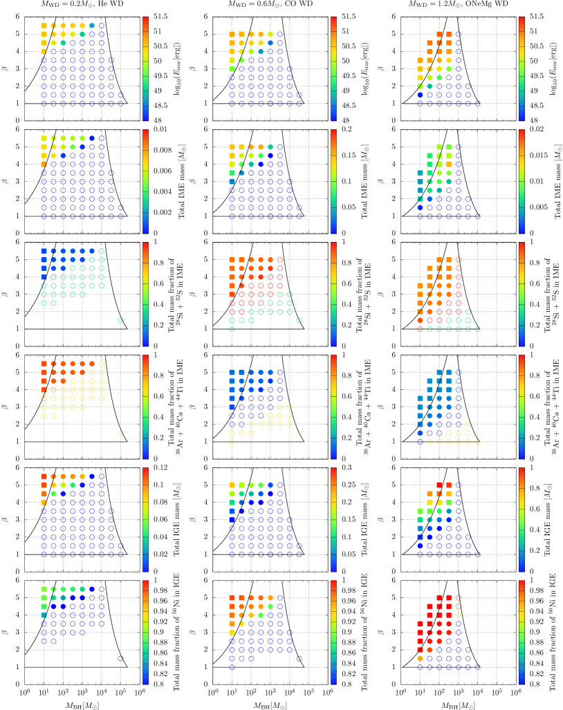
Figure 2: Properties of the TDE debris. The horizontal and vertical axes are the same as Fig. 1, but with the latter in linear scale here. The solid curves also correspond to those in Fig. 1. From left to right, each column shows, respectively, the results for $M_{\textrm{WD}}=0.2$, 0.6, or 1.2 $\mathrm{M}_{\sun}$. The open circles show TDEs without explosive nuclear reactions (Type I), the filled circles are TDEs with the explosive nuclear reactions but without early self-intersection (Type II). The filled squares show TDEs with the explosive nuclear reactions and self-intersection (Type III).

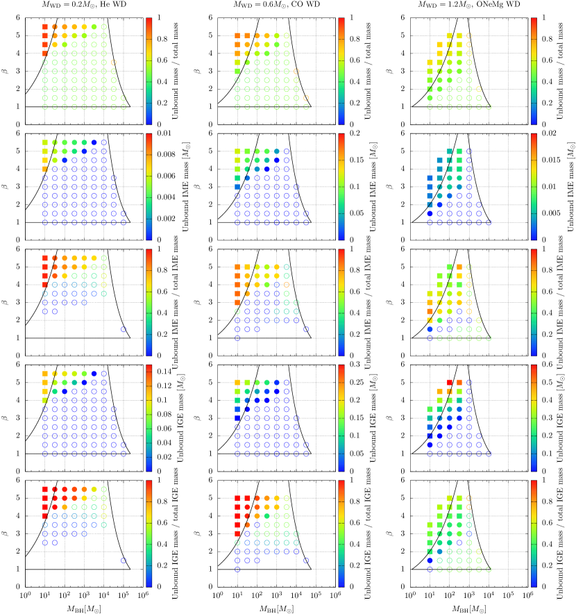
Figure 3: Properties of unbound ejecta. We show the ratio of unbound ejecta mass to the total debris mass, unbound IMEs/IGEs mass, and ratio of unbound IMEs/IGEs mass to the total IMEs/IGEs mass.

3.1 A variety of WD–BH TDEs

Fig. 2 shows the physical properties of total (bound $+$ unbound) debris, while Fig. 3 shows those of unbound debris. The first row in Fig. 2 shows the released nuclear energy $E_{\textrm{nuc}}$. With $E_{\textrm{nuc}}\lesssim 10^{48}$ erg, the nuclear reactions are unimportant, and thus we take this value as the threshold of whether the explosive nuclear reactions occur. Then, our results can be categorized into the following three types.

In Type I TDEs, a WD is tidally disrupted, but explosive nuclear reactions are not ignited. We show the corresponding cases with the open circles in Figs 2 and 3. This type can be considered as an analogue to ordinary TDEs where an MS is disrupted without triggering explosive nuclear reactions.

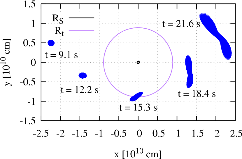
Figure 4: A Type I TDE, where explosive nuclear reactions do not occur. The parameters are $M_{\textrm{WD}}=0.6\,\mathrm{M}_{\sun},\,M_{\textrm{BH}}=10^{3}\,\mathrm{M}_{\sun}$ and $\beta=1.0$.

The other two types show clear signatures of explosive nuclear reactions. The filled points in Figs 2 and 3 represent these types. The difference between the two types is whether early self-intersection occurs. In Type II TDEs, the disrupted WD debris does not hit itself, whereas in Type III, the foregoing part of the debris hits the trailing part. We mark Type II cases, where the self-intersection is not found, with the filled circles in Figs 2 and 3. We show a typical Type II TDE in Fig. 5. Type III TDEs are marked with filled squares in Figs 2 and 3. Although most Type III TDEs are located in the parameter space that is conventionally considered as “a BH enters a WD”, a very small fraction of the WD is swallowed by the BH during the pericentre passage because the BH is much smaller than the WD.

We show an example of Type III in Fig. 6. The left two columns show effects of the self-intersection. The trailing part of the WD intersecting with the advanced part increases the entropy and temperature up to $\sim 2\times 10^{9}$ K, but nuclear reactions are not ignited. The failure of the self-intersection to ignite nuclear reactions is common among all our runs. Thus, the effects of the self-intersection on nuclear reactions are unimportant.

Note that our estimate of the effects of the self-intersection are quantitatively uncertain due to the following two reasons. One reason is that the edges intersecting with each other are under-resolved in SPH methods. The second reason is that SPH particles passing very close to the BH are removed in our methods, which artificially suppresses the innermost self-intersection. This self-intersection would be more violent than what we see currently because bound debris passing closer to the BH have more kinetic energy than debris passing farther. If it is taken into account, the shock would be stronger and might possibly ignite nuclear reactions.

The early self-intersection circularizes the bound debris, which promotes formation of an accretion disc. In Type III TDEs, fallback time-scale of the bound debris is short because the BH masses are small. In Fig. 7, we show the fallback rate calculated from the distribution of specific orbital energy, $\textrm{d}M/\textrm{d}\epsilon$, at the end of the simulation. Here, we take the radiation efficiency as 0.1 and the electron fraction $Y_{\mathrm{e}}$ as 0.5. The peak fallback rate extremely exceeds the Eddington accretion rate. The early self-intersection enables the fallback debris to rapidly circularize and to form an accretion disc (Guillochon et al. 2014; Shiokawa et al. 2015; Guillochon & Ramirez-Ruiz 2015; Bonnerot et al. 2016; for a recent review, see Stone et al. 2018). Thus, we expect that the accretion rate would follow the fallback rate and would exceed super-Eddington accretion rate.

Evans et al. (2015) study a similar kind of TDEs to the Type III TDEs. They simulate TDEs where an MS encounters with an IMBH with $M_{\textrm{BH}}=10^{5}\,\mathrm{M}_{\sun}$ very closely ($\beta=10$ and $15$) although these parameter sets still locate in the “TDE” region in the parameter space shown in Fig. 1. Note that the boundaries shown in Fig. 1 are not for a MS but for WDs. Common properties between their cases and the Type III TDEs are as follows: (1) a very close encounter of a star with a BH, (2) prompt formation of an accretion disc, and (3) highly super-Eddington accretion. A unique point of their cases is that the accretion rates do not follow canonical $t^{-5/3}$ law but remain roughly constant for a few days. They conclude that this is likely due to the strong GR effects.

Despite the similarities, we expect that the accretion rates for the Type III TDEs follow $t^{-5/3}$ law inferred from Fig. 7. This is because the GR effects are unimportant for the Type III TDEs. Because the BH masses are small in the Type III TDEs, the ratio of Schwarzschild radii to the pericentre radii are much smaller than unity. This point shows that the GR effects are unimportant for the Type III TDEs, and the canonical accretion rates proportional to $t^{-5/3}$ would appear.

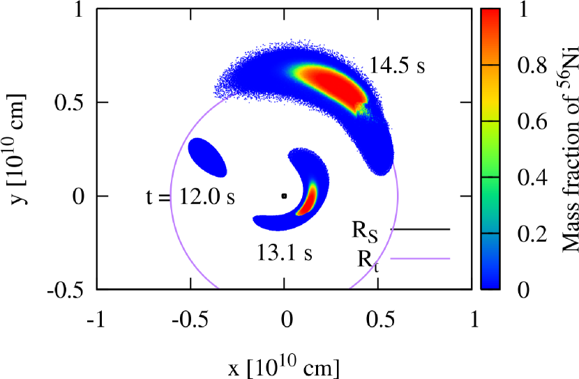
Figure 5: A Type II TDE, where explosive nuclear reactions occur without early self-intersection. The parameters are $M_{\textrm{WD}}=0.6\,\mathrm{M}_{\sun},\,M_{\textrm{BH}}=10^{2.5}\,\mathrm{M}_{\sun}$, and $\beta=5.0$.

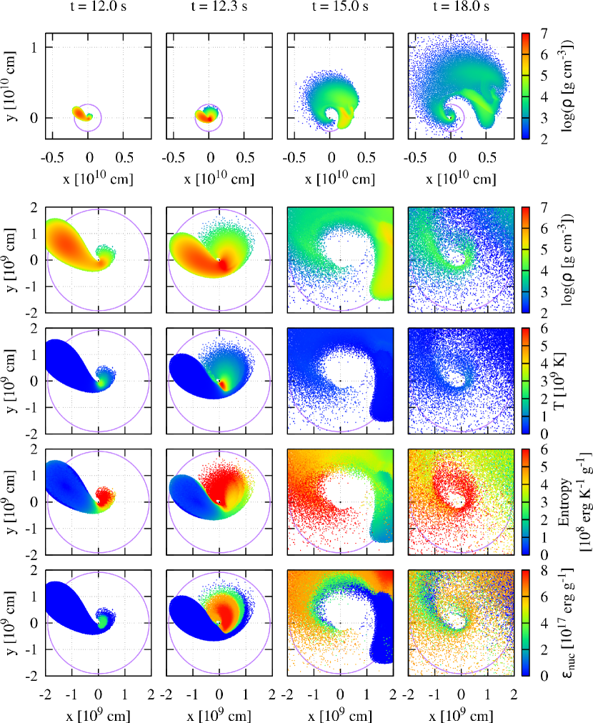
Figure 6: A Type III TDE, where explosive nuclear reactions occur with early self-intersection. The parameters are $M_{\textrm{WD}}=0.6\,\mathrm{M}_{\sun},\,M_{\textrm{BH}}=10\,\mathrm{M}_{\sun}$, and $\beta=5.0$. $t=12.0$ and $12.3$ s are respectively just before and after the self-intersection. The fifth column shows the released specific nuclear energy. The black and purple circles show the Schwarzschild radius and tidal radii respectively. Note that the Schwarzschild radius is very small and hard to see in the figure.

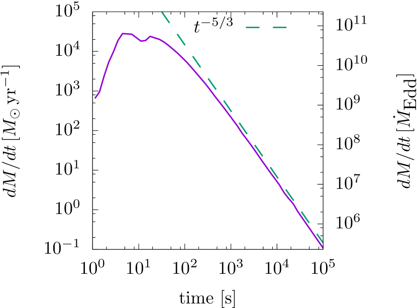
Figure 7: A fallback rate of bound debris for the same case as shown in Fig. 6.

3.2 Abundances

We further study the TDEs with explosive nuclear reactions in detail i.e., the filled points in Fig. 2. The second to fifth rows in Fig. 2 show masses and fractions of nuclear species synthesized. All the debris materials are included, irrespective of bound or unbound. The explosive burning yields a large amount of IGEs, of which more than $80\%$ is ⁵⁶Ni. It is expected that the abundant ⁵⁶Ni in the unbound debris can be a power source in late phases of the TDEs. We will discuss this possibility in Section 5. The elemental abundance depends on $M_{\textrm{WD}}$, but only weakly on $M_{\textrm{BH}}$ and $\beta$. Note that we assume different initial compositions of WDs with different $M_{\textrm{WD}}$. Hence the variety of the final elemental abundance also reflects the initial compositions. The total amount of synthesized elements depends not only on $M_{\textrm{WD}}$ but also on $M_{\textrm{BH}}$ and $\beta$.

Let us first focus on $M_{\textrm{WD}}=0.2\,\mathrm{M}_{\sun}$ cases, where a WD is assumed to consist of pure ⁴He initially. These cases typically produce, (1) a small amount of IMEs, $\lesssim 0.01\,\mathrm{M}_{\sun}$, (2) the IMEs mainly consisting of ³⁶Ar, ⁴⁰Ca, and ⁴⁴Ti, and (3) a relatively low fraction of ⁵⁶Ni, $\lesssim 90\%$ of the IGEs. These features are qualitatively consistent with previous works on nucleosynthesis caused by detonations in light He WDs (Woosley & Weaver, 1994; Livne & Arnett, 1995; Holcomb et al., 2013). Holcomb et al. (2013) study conditions for detonations in light WDs using one-dimensional (1D) hydrodynamics simulations. They find that, if detonation occurs with $\rho_{\textrm{tmax}}\lesssim 10^{6}$ g cm^-3, where $\rho_{\textrm{tmax}}$ is the density at a temperature maximum, the dominant nucleosynthesis products are ⁴⁰Ca, ⁴⁴Ti, and ⁴⁸Cr. Interestingly, we find that the main product from the nucleosynthesis is still ⁵⁶Ni, and that a very small amount of IMEs left with $\lesssim 0.01\,\mathrm{M}_{\sun}$. This is because the part of the disrupted WD that experiences nuclear reactions have densities $\rho_{\textrm{tmax}}\gtrsim 10^{6}$ g cm^-3 in our simulations. Then the main product is ⁵⁶Ni (see Fig. 8).

Our simulations for $M_{\textrm{WD}}=0.6$ and $1.2\,\mathrm{M}_{\sun}$ show that ²⁸Si and ³²S are main IMEs and that most of the IGEs is ⁵⁶Ni ($\gtrsim 95\%$). A notable difference between the two cases is the synthesized amount of IMEs. Roughly $0.1\,\mathrm{M}_{\sun}$ IMEs are synthesized for $M_{\textrm{WD}}=0.6\,\mathrm{M}_{\sun}$ cases, because a significant fraction of the debris experiences incomplete nuclear reactions. For $M_{\textrm{WD}}=1.2\,\mathrm{M}_{\sun}$ cases, nuclear reactions proceed completely and only a small amount ($\simeq 0.01\,\mathrm{M}_{\sun}$) of IMEs are synthesized.

Figure 8: Mass fraction of ⁵⁶Ni and IMEs as functions of the maximum temperature $T_{\textrm{max}}$ of a particle and the density at the moment $\rho_{\textrm{tmax}}$. This is the case of $M_{\textrm{WD}}=0.2\,\mathrm{M}_{\sun},\,M_{\textrm{BH}}=10^{2.5}\,\mathrm{M}_{\sun}$, and $\beta=5.0$.

3.3 Effects of nuclear reactions on motions of debris

The first row in Fig. 3 shows the ratio of unbound ejecta mass to total debris mass. As is naively expected, the unbound mass is larger for larger $E_{\textrm{nuc}}$. A part of the released nuclear energy is converted into orbital energy of the debris. However, for $M_{\textrm{WD}}=1.2\,\mathrm{M}_{\sun}$ cases, the fraction of unbound ejecta does not increase as high as in the cases with lighter WDs. The fifth row in Fig. 3 also shows that the nucleosynthesis products are mostly unbound for the $M_{\textrm{WD}}=0.2$ and 0.6 $\mathrm{M}_{\sun}$ cases, while a significant fraction is bound for the $M_{\textrm{WD}}=1.2\,\mathrm{M}_{\sun}$ cases.

For WDs with $M_{\textrm{WD}}=1.2\,\mathrm{M}_{\sun}$, tidal force redistributes the specific orbital energies more effectively than the released nuclear energy does. The energy spread due to the tidal force $\Delta\epsilon_{t}$ can be estimated as

$$\Delta\epsilon_{t} \sim\beta^{n}\frac{GM_{\textrm{BH}}R_{\textrm{WD}}}{R_{t}^{2}}$$ (5)

$$\simeq 1.2\times 10^{-3}c^{2}\beta^{n}\left(\frac{R_{\textrm{WD}}}{10^{9}\,\textrm{cm}}\right)^{-1}\left(\frac{M_{\textrm{BH}}}{10^{3}\,\mathrm{M}_{\sun}}\right)^{1/3}\left(\frac{M_{\textrm{WD}}}{0.6\,\mathrm{M}_{\sun}}\right)^{2/3},$$ (6)

with $n=2$ for a canonical model, while recent studies (Guillochon & Ramirez-Ruiz, 2013; Stone et al., 2013) show that the value should be revised as $n=0$. Because heavier WDs have smaller radii (see Table 1), $\Delta\epsilon_{t}$ is larger for heavier WDs. If the nuclear reactions advance completely and the compositions become almost pure ⁵⁶Ni, the released specific nuclear energies $\Delta\epsilon_{\textrm{nuc}}$ would be $1.7\times 10^{-3},\,8.7\times 10^{-4}$ and $6.8\times 10^{-4}\,c^{2}$ with the same initial compositions as $M_{\textrm{WD}}=0.2$, 0.6, and $1.2\,\mathrm{M}_{\sun}$ respectively. The effect of the nuclear reactions on the motion of the debris is less important if $\Delta\epsilon_{t}\gg\Delta\epsilon_{\textrm{nuc}}$, and the amount of unbound debris does not significantly increase. In Fig. 9, we show the specific energy distributions given by our simulations. The spreads of the distributions are consistent with Equation (6). We can see that $\Delta\epsilon_{t}\lesssim\Delta\epsilon_{\textrm{nuc}}$ is satisfied for $M_{\textrm{WD}}=0.2$ and $0.6\,\mathrm{M}_{\sun}$ cases. Thus, for those cases, debris where nuclear reactions products IGEs or IMEs are mostly unbound. In contrast, for $M_{\textrm{WD}}=1.2\,\mathrm{M}_{\sun}$ cases, $\Delta\epsilon_{t}\gtrsim\Delta\epsilon_{\textrm{nuc}}$ so that explosive nuclear reactions do not significantly increase the amount of unbound debris and a good fraction of IMEs/IGEs is bound.

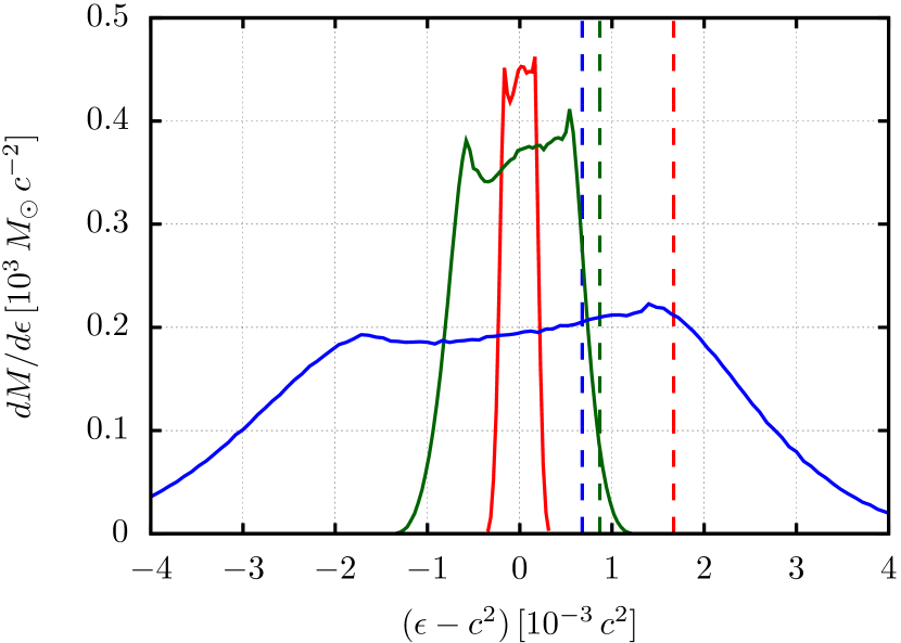
Figure 9: Specific orbital energy distributions after TDEs without explosive nuclear reactions. We compare three cases where $M_{\textrm{WD}}=0.2$ (red), 0.6 (green), and 1.2 $\mathrm{M}_{\sun}$ (blue) and the other parameters are fixed as $M_{\textrm{BH}}=10^{2.5}\,\mathrm{M}_{\sun},$ and $\beta=1.0$. The solid lines express the specific orbital energy distributions, and the dashed lines are the released nuclear specific energies if the compositions become pure ⁵⁶Ni.

4 Resolution dependence

Figure 10: Resolution dependence of nucleosynthesis. Here, the parameters are fixed as $M_{\textrm{BH}}=10^{3}\,\mathrm{M}_{\sun}$ and $\beta=10$ for $M_{\textrm{WD}}=0.2\,\mathrm{M}_{\sun}$, $M_{\textrm{BH}}=10^{3}\,\mathrm{M}_{\sun}$ and $\beta=6$ for $M_{\textrm{WD}}=0.6\,\mathrm{M}_{\sun}$, and $M_{\textrm{BH}}=10^{2.5}\,\mathrm{M}_{\sun}$ and $\beta=3.5$ for $M_{\textrm{WD}}=1.2\,\mathrm{M}_{\sun}$. Note that the number of SPH particles we use in the parameter study is $\simeq 8\times 10^{5}$.

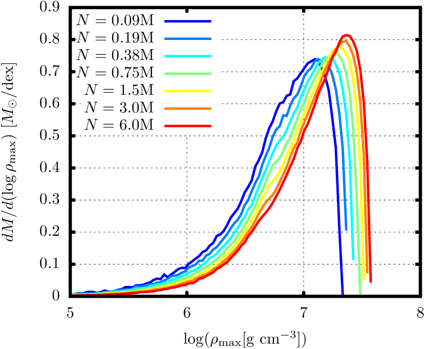
Figure 11: Resolution dependence of $\rho_{\textrm{max}}$. We show distributions of $\rho_{\textrm{max}}$ for the case of $M_{\textrm{WD}}=0.6\,\mathrm{M}_{\sun}$, $M_{\textrm{BH}}=10^{3}\,\mathrm{M}_{\sun}$, and $\beta=5.0$ with different resolutions. We turn off nuclear reactions here.

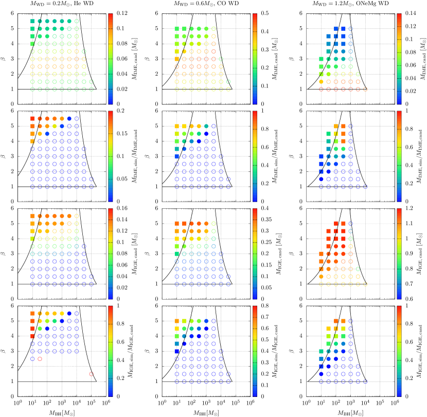
Figure 12: Nucleosynthetic yields independent on resolution of calculations. The first and third rows show the IMEs/IGEs “candidates” masses, or $M_{\mathrm{IME,\,cand}}$/$M_{\mathrm{IGE,\,cand}}$, calculated from distributions of $\rho_{\textrm{max}}$ given by simulations uncoupled with nuclear reactions. The second and fourth rows show ratios of the masses of IMEs/IGEs synthesized in our former calculations coupled with nuclear reactions, or $M_{\mathrm{IME,\,sim}}$/$M_{\mathrm{IGE,\,sim}}$, to $M_{\mathrm{IME,\,cand}}$/$M_{\mathrm{IGE,\,cand}}$.

Tanikawa et al. (2017) perform simulations of WD–BH TDEs where nuclear reactions ignite, using almost the same methods as ours. Specifically, they take parameters as $M_{\textrm{BH}}=500\,\mathrm{M}_{\sun},\,\beta=5$ for He/CO WD cases and $M_{\textrm{BH}}=100\mathrm{M}_{\sun},\,\beta=3$ for ONeMg WD cases. They examine convergence of nucleosynthesis varying the number of the SPH particles up to 25 million. The results do not converge in all the cases. They show that spurious heating due to low resolution ignite nuclear burning. They additionally perform 1D simulations with high resolution where initial conditions are taken from three-dimensional (3D) SPH simulations uncoupled with nuclear reactions. In the 1D simulations, shock wave triggers detonation instead of spurious heating. However, the 1D initial conditions are not so accurate that we cannot precisely determine where a shock wave emerges.

We examine the resolution dependence of our nucleosynthesis results, which is shown in Fig. 10. Here, we take the simulation parameters such that $\beta$ takes the maximum value among the Type II TDEs in order to avoid the effects of the early self-intersection and in order to examine the effects of the failure to resolve the maximum compression point. Fig. 10 shows that our results do not converge, although the degree of resolution dependence varies depending on the WD masses. Our results are consistent with those of Tanikawa et al. (2017), in which different simulation parameters are used. The result shown in Fig. 10 renders our results of nucleosynthesis to remain uncertain.

In order to examine the validity of our results, we estimate the nucleosynthetic yields in a different way and compare the both yields given in the two different ways. To this end, we need a physical quantity that indicates nucleosynthetic yields, is not affected by the spurious heating, and thus is robust. Naively, the temperature and density when nuclear reactions occur are key physical quantities associated with the nucleosynthesis (see Fig. 8). However, the numerical heating critically affects $T_{\textrm{max}}$ and $\rho_{\textrm{tmax}}$, and we cannot use these values.

Instead, we additionally perform SPH simulations in which the nuclear reactions are turned off, and record the maximum density of each SPH particle during the simulation, $\rho_{\textrm{max}}$, to derive nucleosynthetic yields. Most of the SPH particles have the maximum density $\rho_{\textrm{max}}$ when the tidal compression is the strongest; then the nuclear burning would be the most violent if it happen. We show the resolution dependence of $\rho_{\textrm{max}}$ in Fig. 11, which shows that the distribution of $\rho_{\textrm{max}}$ indeed converges.

We estimate the elemental abundances as functions of initial compositions and $\rho_{\textrm{max}}$ in Table 2. The table is based on the results of Fink et al. (2010), Holcomb et al. (2013), and Marquardt et al. (2015). Fink et al. (2010), and Marquardt et al. (2015) estimate the elemental abundances as functions of fuel density in detonations in Type Ia SNe by iterating hydrodynamical simulations of WD explosions and post-processing nuclear reaction calculations. Fink et al. (2010) derive corresponding functions for the helium and carbon/oxygen detonation, while Marquardt et al. (2015) study detonation for initial composition of $X(^{12}\mathrm{C})=0.03$, $X(^{16}\mathrm{O})=0.6$, and $X(^{20}\mathrm{Ne})=0.07$. We apply these results for our CO and ONeMg WD cases. For He WD cases, we apply the results of Holcomb et al. (2013) and ours shown in Fig. 8. Our approximation to the results is listed in Table 2. We calculate nucleosynthetic yields using Table 2, assuming that the whole WD experiences detonation and nuclear burning at the maximum compression point with the density $\rho_{\textrm{max}}$.

The results are shown in Fig. 12. Note that the masses of IMEs/IGEs obtained in this way are those of IMEs/IGEs “candidates”, or $M_{\mathrm{IME,\,cand}}$/$M_{\mathrm{IGE,cand}}$, because we assume the whole WD burns. If a part of the WD does not burn or produce IMEs or IGEs, the IMEs/IGEs masses are smaller than $M_{\mathrm{IME,\,cand}}$/$M_{\mathrm{IGE,\,cand}}$. In this sense, we can regard $M_{\mathrm{IME,\,cand}}$/$M_{\mathrm{IGE,\,cand}}$ as upper limits of the IMEs/IGEs masses. Fig. 12 also shows the ratios of the masses of IMEs/IGEs synthesized in our former simulations coupled with nuclear reactions, or $M_{\mathrm{IME,\,sim}}$/$M_{\mathrm{IGE,\,sim}}$, to $M_{\mathrm{IME,\,cand}}$/$M_{\mathrm{IGE,\,cand}}$. In all the cases, the ratios are smaller than unity, which means that $M_{\mathrm{IME,\,sim}}<M_{\mathrm{IME,\,cand}}$ and $M_{\mathrm{IGE,\,sim}}<M_{\mathrm{IGE,\,cand}}$ are satisfied. In many cases, the synthesized amounts are remarkably similar to the results shown in Fig. 2, especially in runs with large $\beta$ and small $M_{\textrm{BH}}$. Although there are cases where $M_{\mathrm{IME,\,cand}}$/$M_{\mathrm{IGE,\,cand}}$ are significantly larger than $M_{\mathrm{IME,\,sim}}$/$M_{\mathrm{IGE,\,sim}}$, this is largely because of our assumption adopted here that the whole WD is burned. Therefore, while there still remain uncertainties in the nucleosynthesis calculations presented in Section 3, the numerical resolution issue does not completely ruin our main conclusion that WD–BH TDEs produce a variety of events. The diversity is at least qualitatively represented by our series of hydrodynamics simulations.

The “candidates” masses are robust because of their convergence. Fig. 12 shows that they have a wide range, potentially indicating that there would be a variety of the amounts of IMEs/IGEs synthesized. The ratios $M_{\mathrm{IME,\,sim}}/M_{\mathrm{IME,\,cand}}$ and $M_{\mathrm{IGE,\,sim}}/M_{\mathrm{IGE,\,cand}}$ are still uncertain, and should be derived with extremely high-resolution studies, such as Tanikawa (2017b). Tanikawa (2017b) perform 3D hydrodynamical simulations of He WD–IMBH TDEs uncoupled with nuclear reactions and multiple 1D high-resolution simulation coupled with nuclear reactions for one parameter set. They investigate which part of the WD experiences detonation with multiple 1D simulations, and give amounts of synthesized elements. However, it is hard to perform such numerically expensive simulations for various cases of WD–BH TDEs and to explore the variety of the amounts.

Table 2: Nucleosynthetic yields as functions of initial compositions and $\rho_{\textrm{max}}$. $X_{\mathrm{IME}}$, $X_{\mathrm{IGE}}$ are respectively mass fractions of IMEs/IGEs after nuclear burning.

Composition	$\rho_{\max}$ (g cm-3)	$X_{\mathrm{IME}}$	$X_{\mathrm{IGE}}$
He	$\rho_{\max}\leq 10^{5}$	0	0
	$10^{5}<\rho_{\max}\leq 5\times 10^{5}$	0.6	0
	$5\times 10^{5}<\rho_{\max}$	0	1.0
CO	$\rho_{\max}\leq 2\times 10^{5}$	0	0
	$2\times 10^{5}<\rho_{\max}\leq 2\times 10^{6}$	0.4	0
	$2\times 10^{6}<\rho_{\max}\leq 10^{7}$	0.9	0.1
	$10^{7}<\rho_{\max}$	0	1.0
ONeMg	$\rho_{\max}\leq 2\times 10^{5}$	0	0
	$2\times 10^{5}<\rho_{\max}\leq 2\times 10^{6}$	0.15	0
	$2\times 10^{6}<\rho_{\max}\leq 10^{7}$	0.8	0
	$10^{7}<\rho_{\max}$	0	1.0

5 Conclusions

We have performed a large number of simulations of WD–BH TDEs with a wide variety of the WD mass, BH mass and the initial orbital parameters. We find that, when explosive nuclear reactions occur, a significant mass fraction of a WD, up to a few tens percent, is converted into IGEs. Most of them are gravitationally unbound, and radioactive decay of ⁵⁶Ni in the unbound ejecta would cause a transient event similar to Type I SNe (MacLeod et al., 2016). The released nuclear energy increases the fraction of unbound debris, but the effect is less important for heavier WDs because the distribution of specific energies of the debris is determined by the tidal force rather than nuclear reactions.

There still remain uncertainties in our nucleosynthesis results due to inadequate resolution in our hydrodynamical simulations coupled with nuclear reactions. In many cases, however, the synthesized elements masses are quite similar to upper limits of them obtained by a robust method with which we can avoid the uncertainties. The results derived in the two different ways consistently show that WD–BH TDEs produce a wide variety of nucleosynthetic yields.

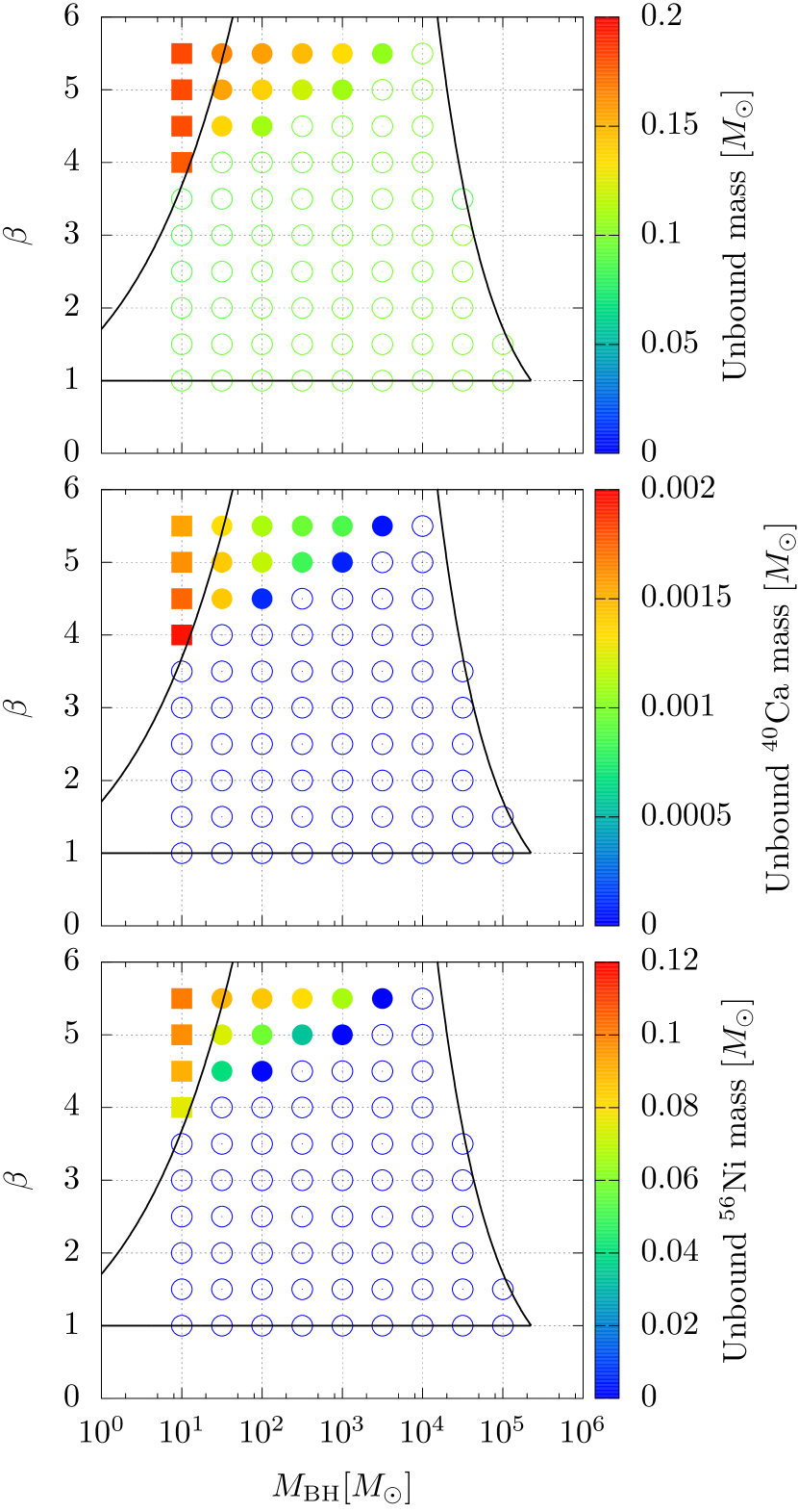
Figure 13: Properties related to calcium-rich gap transients. We show the $0.2\,\mathrm{M}_{\sun}$ WD cases here.

Sell et al. (2015) argue that a TDE of a light WD mainly composed of ⁴He by an IMBH can be a progenitor of calcium-rich gap transients. Kasliwal et al. (2012) show properties of the transients: they are similar to Type I SNe, but are faint, with high velocities, very large calcium abundances, and faster evolution than average Type Ia SNe. Calcium-rich gap transients are found typically in the outskirts of known galaxies. We can derive the elemental abundances after TDEs where a $0.2\,\mathrm{M}_{\sun}$ WD is disrupted. Fig. 13 shows the masses of ⁴⁰Ca and ⁵⁶Ni in unbound ejecta. ⁴⁰Ca accounts for a tiny fraction of the ejecta ($\lesssim$1 %), while ⁵⁶Ni does a large fraction ($\simeq$50 %) in the Type II and III TDEs. The large masses of ⁵⁶Ni ($\gtrsim 0.04\,\mathrm{M}_{\sun}$) do not match with the estimated ⁵⁶Ni masses in observed calcium-rich gap transients, such as 0.003 $\mathrm{M}_{\sun}$ for SN2005E (Perets et al., 2010), 0.016 $\mathrm{M}_{\sun}$ for PTF10iuv (Kasliwal et al., 2012), and 0.005-0.010$~{}\mathrm{M}_{\sun}$ for SN2012hn (Valenti et al., 2014). We do not find WD–BH TDEs that can be a progenitor of calcium–rich gap transients. This is because the WD is so strongly compressed by the tidal force that $\rho_{\textrm{tmax}}$ reaches $\gtrsim 10^{6}$ g cm^-3, the explosive nuclear reactions leave a small amount of IMEs ($\lesssim 0.01\,\mathrm{M}_{\sun}$) and a large amount of IGEs ($\sim 0.1\,\mathrm{M}_{\sun}$).

In the cases of Type III TDEs where the early self-intersection occurs, extremely super-Eddington accretion rates would be realized. In such situations, there would be relativistic winds and/or jets driven by radiation pressure, and these events could be so-called jetted TDEs (Strubbe & Quataert, 2009; Coughlin & Begelman, 2014; Shen & Matzner, 2014; Coughlin & Begelman, 2015; Lu et al., 2017). An observer along with the jet axis would see beamed emission resembling ultra-long $\gamma$-ray bursts that would be observable even if the events are very distant. For example, MacLeod et al. (2016) estimate that events with the jet luminosity of $10^{49}\,\mathrm{erg}\,\mathrm{s}^{-1}$ would be observable up to the redshift of 2.45 with Swift Burst Alert Telescope.

We have explored the diversity WD–BH TDEs caused by the combination of the physical parameters, $M_{\textrm{WD}}$, $M_{\textrm{BH}}$, and $\beta$. The variety of TDEs may show a wealth of phenomena observationally. MacLeod et al. (2016) perform radiative transfer calculations using the results of hydrodynamical simulations of Rosswog et al. (2009). They find that a single TDE can show different observational signatures depending on the viewing angle. We plan to perform detailed radiative transfer calculations to derive the spectral energy distributions and light curves in our future work.

References

- Bauer et al. (2017) Bauer F. E., et al., 2017, MNRAS, 467, 4841
- Bicknell & Gingold (1983) Bicknell G. V., Gingold R. A., 1983, ApJ, 273, 749
- Bloom et al. (2011) Bloom J. S., et al., 2011, Science, 333, 203
- Bogdanović et al. (2004) Bogdanović T., Eracleous M., Mahadevan S., Sigurdsson S., Laguna P., 2004, ApJ, 610, 707
- Bonnerot et al. (2016) Bonnerot C., Rossi E. M., Lodato G., Price D. J., 2016, MNRAS, 455, 2253
- Brown et al. (2015) Brown G. C., Levan A. J., Stanway E. R., Tanvir N. R., Cenko S. B., Berger E., Chornock R., Cucchiaria A., 2015, MNRAS, 452, 4297
- Burrows et al. (2011) Burrows D. N., et al., 2011, Nature, 476, 421
- Carter & Luminet (1982) Carter B., Luminet J. P., 1982, Nature, 296, 211
- Cenko et al. (2012) Cenko S. B., et al., 2012, ApJ, 753, 77
- Cheng & Bogdanović (2014) Cheng R. M., Bogdanović T., 2014, Phys. Rev. D, 90, 064020
- Clausen & Eracleous (2011) Clausen D., Eracleous M., 2011, ApJ, 726, 34
- Coughlin & Begelman (2014) Coughlin E. R., Begelman M. C., 2014, ApJ, 781, 82
- Coughlin & Begelman (2015) Coughlin E. R., Begelman M. C., 2015, ApJ, 809, 2
- Dehnen & Aly (2012) Dehnen W., Aly H., 2012, MNRAS, 425, 1068
- East (2014) East W. E., 2014, ApJ, 795, 135
- Evans et al. (2015) Evans C., Laguna P., Eracleous M., 2015, ApJ, 805, L19
- Fink et al. (2010) Fink M., Röpke F. K., Hillebrandt W., Seitenzahl I. R., Sim S. A., Kromer M., 2010, A&A, 514, A53
- Giannios & Metzger (2011) Giannios D., Metzger B. D., 2011, MNRAS, 416, 2102
- Guillochon & Ramirez-Ruiz (2013) Guillochon J., Ramirez-Ruiz E., 2013, ApJ, 767, 25
- Guillochon & Ramirez-Ruiz (2015) Guillochon J., Ramirez-Ruiz E., 2015, ApJ, 809, 166
- Guillochon et al. (2014) Guillochon J., Manukian H., Ramirez-Ruiz E., 2014, ApJ, 783, 23
- Haas et al. (2012) Haas R., Shcherbakov R. V., Bode T., Laguna P., 2012, ApJ, 749, 117
- Hayasaki et al. (2016) Hayasaki K., Stone N., Loeb A., 2016, MNRAS, 461, 3760
- Holcomb et al. (2013) Holcomb C., Guillochon J., De Colle F., Ramirez-Ruiz E., 2013, ApJ, 771, 14
- Ioka et al. (2016) Ioka K., Hotokezaka K., Piran T., 2016, ApJ, 833, 110
- Iwasawa et al. (2016a) Iwasawa M., Tanikawa A., Hosono N., Nitadori K., Muranushi T., Makino J., 2016a, FDPS: Framework for Developing Particle Simulators, Astrophysics Source Code Library (ascl:1604.011)
- Iwasawa et al. (2016b) Iwasawa M., Tanikawa A., Hosono N., Nitadori K., Muranushi T., Makino J., 2016b, PASJ, 68, 54
- Jiang et al. (2016) Jiang Y.-F., Guillochon J., Loeb A., 2016, ApJ, 830, 125
- Jonker et al. (2013) Jonker P. G., et al., 2013, ApJ, 779, 14
- Kasliwal et al. (2012) Kasliwal M. M., et al., 2012, ApJ, 755, 161
- Kobayashi et al. (2004) Kobayashi S., Laguna P., Phinney E. S., Mészáros P., 2004, ApJ, 615, 855
- Komossa (2015) Komossa S., 2015, Journal of High Energy Astrophysics, 7, 148
- Krolik & Piran (2011) Krolik J. H., Piran T., 2011, ApJ, 743, 134
- Krolik et al. (2016) Krolik J., Piran T., Svirski G., Cheng R. M., 2016, ApJ, 827, 127
- Law-Smith et al. (2017) Law-Smith J., MacLeod M., Guillochon J., Macias P., Ramirez-Ruiz E., 2017, ApJ, 841, 132
- Levan et al. (2011) Levan A. J., et al., 2011, Science, 333, 199
- Livne & Arnett (1995) Livne E., Arnett D., 1995, ApJ, 452, 62
- Lodato & Rossi (2011) Lodato G., Rossi E. M., 2011, MNRAS, 410, 359
- Loeb & Ulmer (1997) Loeb A., Ulmer A., 1997, ApJ, 489, 573
- Lu et al. (2017) Lu W., Krolik J., Crumley P., Kumar P., 2017, MNRAS, 471, 1141
- Luminet & Pichon (1989a) Luminet J.-P., Pichon B., 1989a, A&A, 209, 85
- Luminet & Pichon (1989b) Luminet J.-P., Pichon B., 1989b, A&A, 209, 103
- MacLeod et al. (2014) MacLeod M., Goldstein J., Ramirez-Ruiz E., Guillochon J., Samsing J., 2014, ApJ, 794, 9
- MacLeod et al. (2016) MacLeod M., Guillochon J., Ramirez-Ruiz E., Kasen D., Rosswog S., 2016, ApJ, 819, 3
- Mainetti et al. (2017) Mainetti D., Lupi A., Campana S., Colpi M., Coughlin E. R., Guillochon J., Ramirez-Ruiz E., 2017, A&A, 600, A124
- Marquardt et al. (2015) Marquardt K. S., Sim S. A., Ruiter A. J., Seitenzahl I. R., Ohlmann S. T., Kromer M., Pakmor R., Röpke F. K., 2015, A&A, 580, A118
- Metzger & Stone (2016) Metzger B. D., Stone N. C., 2016, MNRAS, 461, 948
- Monaghan (1997) Monaghan J. J., 1997, Journal of Computational Physics, 136, 298
- Perets et al. (2010) Perets H. B., et al., 2010, Nature, 465, 322
- Piran et al. (2015) Piran T., Svirski G., Krolik J., Cheng R. M., Shiokawa H., 2015, ApJ, 806, 164
- Price & Monaghan (2007) Price D. J., Monaghan J. J., 2007, MNRAS, 374, 1347
- Rees (1988) Rees M. J., 1988, Nature, 333, 523
- Rosswog et al. (2008) Rosswog S., Ramirez-Ruiz E., Hix W. R., 2008, ApJ, 679, 1385
- Rosswog et al. (2009) Rosswog S., Ramirez-Ruiz E., Hix W. R., 2009, ApJ, 695, 404
- Roth & Kasen (2017) Roth N., Kasen D., 2017, preprint, (arXiv:1707.02993)
- Roth et al. (2016) Roth N., Kasen D., Guillochon J., Ramirez-Ruiz E., 2016, ApJ, 827, 3
- Sato et al. (2015) Sato Y., Nakasato N., Tanikawa A., Nomoto K., Maeda K., Hachisu I., 2015, ApJ, 807, 105
- Sato et al. (2016) Sato Y., Nakasato N., Tanikawa A., Nomoto K., Maeda K., Hachisu I., 2016, ApJ, 821, 67
- Sell et al. (2015) Sell P. H., Maccarone T. J., Kotak R., Knigge C., Sand D. J., 2015, MNRAS, 450, 4198
- Shapiro & Teukolsky (1983) Shapiro S. L., Teukolsky S. A., 1983, Black holes, white dwarfs, and neutron stars: The physics of compact objects. Wiley
- Shcherbakov et al. (2013) Shcherbakov R. V., Pe’er A., Reynolds C. S., Haas R., Bode T., Laguna P., 2013, ApJ, 769, 85
- Shen & Matzner (2014) Shen R.-F., Matzner C. D., 2014, ApJ, 784, 87
- Shiokawa et al. (2015) Shiokawa H., Krolik J. H., Cheng R. M., Piran T., Noble S. C., 2015, ApJ, 804, 85
- Stone et al. (2013) Stone N., Sari R., Loeb A., 2013, MNRAS, 435, 1809
- Stone et al. (2018) Stone N. C., Kesden M., Cheng R. M., van Velzen S., 2018, preprint, (arXiv:1801.10180)
- Strubbe & Quataert (2009) Strubbe L. E., Quataert E., 2009, MNRAS, 400, 2070
- Tanikawa (2017b) Tanikawa A., 2017b, preprint, (arXiv:1711.05451)
- Tanikawa (2017a) Tanikawa A., 2017a, preprint, (arXiv:1711.07115)
- Tanikawa et al. (2012) Tanikawa A., Yoshikawa K., Okamoto T., Nitadori K., 2012, New Astron., 17, 82
- Tanikawa et al. (2013) Tanikawa A., Yoshikawa K., Nitadori K., Okamoto T., 2013, New Astron., 19, 74
- Tanikawa et al. (2015) Tanikawa A., Nakasato N., Sato Y., Nomoto K., Maeda K., Hachisu I., 2015, ApJ, 807, 40
- Tanikawa et al. (2017) Tanikawa A., Sato Y., Nomoto K., Maeda K., Nakasato N., Hachisu I., 2017, ApJ, 839, 81
- Tejeda & Rosswog (2013) Tejeda E., Rosswog S., 2013, MNRAS, 433, 1930
- Timmes & Swesty (2000) Timmes F. X., Swesty F. D., 2000, ApJS, 126, 501
- Timmes et al. (2000) Timmes F. X., Hoffman R. D., Woosley S. E., 2000, ApJS, 129, 377
- Valenti et al. (2014) Valenti S., et al., 2014, MNRAS, 437, 1519
- Wendland (1995) Wendland H., 1995, Advances in computational Mathematics, 4, 389
- Woosley & Weaver (1994) Woosley S. E., Weaver T. A., 1994, ApJ, 423, 371
- Zalamea et al. (2010) Zalamea I., Menou K., Beloborodov A. M., 2010, MNRAS, 409, L25
- Zauderer et al. (2011) Zauderer B. A., et al., 2011, Nature, 476, 425