Data clustering with edge domination in complex networks

Abstract

This paper presents a model for a dynamical system where particles dominate edges in a complex network. The proposed dynamical system is then extended to an application on the problem of community detection and data clustering. In the case of the data clustering problem, 6 different techniques were simulated on 10 different datasets in order to compare with the proposed technique. The results show that the proposed algorithm performs well when prior knowledge of the number of clusters is known to the algorithm.

1 Introduction

Consider a dataset that is represented by a weighted, undirected graph where a vertex represents a data point and an edge a relationship of similarity. Particularly, if a dynamical system can take place in this graph representation then this graph can be studied with tools of the complex network theory [2].

In machine learning, methods that are based on networks have increasingly being studied. The representation of a dataset as a network allows the method to work not only with a similarity score among pairs of nodes, but it also provides a topological information. Within this context, the goal of this paper is to present a dynamical system of particle competition system on edges of complex networks for the community detection and the data clustering problem.

Regarding previous work with semi-supervised learning, in this paper the presented model modifies dynamics of particle generation and introduces the information of weights in edges. In Section 2 the model is introduced with an overview and a mathematical description. In Section 3 simulations on a real network, artificial datasets, and real-world datasets are presented. Finally in Section 4, some final considerations regarding the studied model are discussed.

2 Edge Domination System

In this section, I give an introduction to the proposed technique, namely Edge Domination System. First an overview and then its mathematical modeling.

2.1 Overview

Consider a complex network expressed by a simple, undirected, weighted graph $G=(\mathcal{V},\mathcal{E})$, where $\mathcal{V}$ is the set of vertices and $\mathcal{E}\subseteq\mathcal{V}\times\mathcal{V}$ is the set of edges. If two vertices are considered similar, then they are connected by an edge. Denote $(i,j)$ to be the edge between vertices $v_{i}$ and $v_{j}$, which has a weight $\mathcal{W}(i,j)\in\mathbb{R}$. The weights represent the similarity between two vertices where a larger value indicates higher similarity. The graph that expresses this network is represented by the weighted adjacency matrix $W=(w_{ij})$ where $w_{ij}=w_{ji}=\mathcal{W}(i,j)$ if $v_{i}$ is connected to $v_{j}$ and zero otherwise. The process’ result consists of $K$ groups of vertices that are not necessarily connected.

In this model, particles are the objects that flow within the network. Every particle belongs to a class, defined at time of their creation. After being released in any node of the network, a particle randomly walks the network. The probability among adjacent vertices to be chosen as the next vertex follows the distribution of the weights of the possible edges. Consider a particle that is in $v_{i}$. This particle decides to move to $v_{j}$ with probability

$$w_{ij}\cdot\left(\sum_{k=1}^{|\mathcal{V}|}w_{ik}\right)^{\!-1}\mbox{.}$$

The particle’s decision, however, does not imply it will succeed at moving to the neighboring vertex. If the edge that is connecting this vertex has been visited by particles of different classes, this particle might be absorbed before reaching the vertex and then it will cease to affect the system. If the particle succeeds at moving to the neighboring vertex, it is said that this particle has survived—and it will continue walking through the network. This walking dynamics is modeled in terms of level of subordination and domination of a class in relation to all other classes of particles.

In order to determine the level of domination and subordination of each class in an edge we observe the active particles at a given time in the system. Define current directed domination $\tilde{n}^{c}_{ij}(t)$ to be the number of active particles that belong to class $c$ that have decided to move from $v_{i}$ to $v_{j}$ at time $t$ and survived. Similarly, define current relative subordination $\tilde{\sigma}^{c}_{ij}$ to be the fraction of active particles that do not belong to class $c$ and have successfully passed through edge $(i,j)$ regardless of direction at time $t$. The latter is defined as

$$\tilde{\sigma}^{c}_{ij}\coloneqq\begin{dcases*}1-\frac{\tilde{n}^{c}_{ij}+\tilde{n}^{c}_{ji}}{\sum_{q=1}^{K}{\left(\tilde{n}^{q}_{ij}+\tilde{n}^{q}_{ji}\right)}}&if $\tilde{n}^{q}_{ij}+\tilde{n}^{q}_{ji}>0,\forall q$\mbox{,}\\ \frac{1}{K}&otherwise.\end{dcases*}$$

The survival of a particle depends on the current relative domination of the edge and the destination vertex. The survival probability is

$$1-\lambda\tilde{\sigma}^{c}_{ij}(t)$$

where $\lambda\in[0,1]$ is the competition parameter.

Since particles are absorbed through the dynamics of competition, a mechanism to perform replacement of absorbed particles is needed in order to avoid a state where there are no active particles in the system. This replacement is done by creating new particles according to the distribution of the current active particles of a given class in the system.

Let $n^{c}_{i}(t)$ be the number of active particles that belong to class $c$ at time $t$. The number of new particles that will belong to class $c$ in $v_{i}$ at time $t$ follows the distribution

$$\begin{dcases*}\mathrm{B}\!\left(\left\lfloor\tilde{n}^{c}(0)-\tilde{n}^{c}(t)\right\rfloor,~{}\rho^{c}_{i}\right)&if $\left\lfloor\tilde{n}^{c}(0)-\tilde{n}^{c}(t)\right\rfloor>0$,\\ \mathrm{B}(1,0)&otherwise,\end{dcases*}$$

where

$$\rho^{c}_{i}\coloneqq\frac{\tilde{n}^{c}_{i}}{\sum_{j=1}^{|V|}{\tilde{n}^{c}_{j}}}$$

and $\mathrm{B}(n,p)$ is a binomial distribution. In other words, if the number of active particles is less than the initial number of active particles, then it is performed $\left\lfloor\tilde{n}^{c}(0)-\tilde{n}^{c}(t)\right\rfloor$ trials with probability $\rho^{c}_{i}$ at generating a new particle in $v_{i}$.

It follows that the expected number of new particles that belong to class $c$ in $v_{i}$ at time $t$ is

$$\begin{dcases}\rho^{c}_{i}\left\lfloor\tilde{n}^{c}(0)-\tilde{n}^{c}(t)\right\rfloor&\mbox{if }\left\lfloor\tilde{n}^{c}(0)-\tilde{n}^{c}(t)\right\rfloor>0\mbox{,}\\ 0&\mbox{otherwise.}\end{dcases}$$

The information of the current directed domination $\tilde{n}^{c}_{ij}(t)$ determines the class of particles that dominates each edge in the system. The edges of the network are grouped in sets by the class that dominates them. For each class $c$, the subset of edges $\mathcal{E}^{c}(t)\in\mathcal{E}$ is

$$\mathcal{E}^{c}(t)\coloneqq\left\{ij\middle|\operatorname*{arg\,max}_{q}\!{\left(\tilde{n}^{q}_{ij}(t)+\tilde{n}^{q}_{ji}(t)\right)=c}\right\}\mbox{.}$$

Define the unweighted subnetwork

$$G^{c}(t)\coloneqq\left(\mathcal{V},\mathcal{E}^{c}(t)\right)$$ (1)

to be the unfolding of network $G$ according to class $c$ at time $t$. This subnetwork can be interpreted as a subspace with the most relevant relationships for a given class. The available information in these subnetworks will be utilized for the study of community detection and data clustering.

Next, a formal modeling of this dynamical system is presented.

2.2 Mathematical Modeling

Formally, we define Edge Domination System as a dynamical system $\tilde{X}(t)$. Let $\tilde{n}^{c}_{i}(t)$ be the number of active particles that belong to class $c$ in $v_{i}$ at time $t$. The internal state of this dynamical system is

$$\tilde{X}(t)\coloneqq\left[\,\vec{\tilde{n}}^{c}(t)\,\right]^{T}\!\mbox{,}$$ (2)

where

$$\vec{\tilde{n}}^{c}(t)\coloneqq\big{[}\,\tilde{n}^{c}_{i}(t)\,\big{]}_{i}\,\mbox{.}$$

Let $\tilde{g}^{c}_{i}(t)$ and $\tilde{a}^{c}_{i}(t)$ be, respectively, the number of particles generated and absorbed in $v_{i}$ at time $t$. The evolution function $\tilde{\phi}$ of the dynamical system is

$$\tilde{\phi}:\begin{dcases}\tilde{n}^{c}_{i}(t+1)=\tilde{n}^{c}_{i}(t)+\sum_{j}{\left(\tilde{n}^{c}_{ji}(t+1)-\tilde{n}^{c}_{ij}(t+1)\right)}+\tilde{g}^{c}_{i}(t+1)-\tilde{a}_{i}^{c}(t+1)\,\mbox{.}\end{dcases}$$

Intuitively, the number $\tilde{n}^{c}_{i}$ of active particles that are in a vertex is the total number of particles arriving minus the number of particles leaving and particles the have been absorbed. Additionally, there is a term for the number $\tilde{g}^{c}_{i}$ of generated particles. Values $\tilde{n}^{c}_{ij}$, $\tilde{g}^{c}_{i}$, and $\tilde{a}^{c}_{i}$ are obtained stochastically according to the dynamics of walking, absorption, and generation. The initial state of the system is given by an arbitrary number $\tilde{n}^{c}_{i}(0)$ of initial active particles and $\tilde{n}^{c}_{ij}(0)=0$.

In order to achieve the desirable network unfolding, it is necessary to average the results of several simulations of the system with a very large number of initial particles $\tilde{n}^{c}_{i}(0)$. However, the computational cost of a such simulation is very high. Alternatively, a system $X(t)$ that achieves similar results in a deterministic manner can be modeled. This alternative system considers that exists an asymptotically infinite number of initial active particles.

2.3 Alternative Mathematical Modeling

Consider the dynamical system whose internal state is

$$X(t)\coloneqq\begin{bmatrix}\vec{n}^{c}(t)=\big{[}n^{c}_{i}(t)\big{]}_{i}\\[7.22743pt] N^{c}(t)=\big{(}n^{c}_{ij}(t)\big{)}_{ij}\\[7.22743pt] \end{bmatrix}$$

that is a nonlinear Markovian dynamical system with the deterministic evolution function

$$\phi\colon\begin{dcases}\vec{n}^{c}(t+1)=\vec{n}^{c}(t)\times P^{c}(X(t))\left(\vec{n}^{c}(t)\times P^{c}(X(t))\cdot\vec{1}\right)^{-1}\\ N^{c}(t+1)=\operatorname{diag}{\vec{n}^{c}(t)}\times P^{c}(X(t))\,\mbox{,}\\ \end{dcases}$$ (3)

where

$$P^{c}(X)\coloneqq\Big{(}p^{c}_{ij}(X)\Big{)}_{ij}\mbox{,}$$

$$p^{c}_{ij}(X)\coloneqq\frac{w_{ij}}{\sum_{k=1}^{|V|}w_{ik}}\left(1-\lambda\sigma^{c}_{ij}(X)\right)\mbox{,}$$ (4)

$$\sigma^{c}_{ij}(X)\coloneqq\begin{dcases*}1-\frac{n^{c}_{ij}+n^{c}_{ji}}{\sum_{q=1}^{K}{\left(n^{q}_{ij}+n^{q}_{ji}\right)}}&if $n^{c}_{ij}+n^{c}_{ji}>0$, $\forall c$,\\ \frac{1}{K}&otherwise.\end{dcases*}$$ (5)

The initial state of system $X$ is given by an arbitrary discrete distribution $\vec{n}^{c}(0)$ of initial active particles and $n^{c}_{ij}(0)=0$. This system performs an unfolding in $\mathcal{O}(K|\mathcal{E}|)$ operations.

2.4 Community Detection

In the context of community detection, we simulate the alternative model with $K$ classes—here $K$ is also the number of communities—up to time T and work with the unweighted subnetworks $G^{c}(T)$ in order to determine the community structure within the network $G$. A vertex is said to belong to community $c$ if the density of edges in a neighborhood is higher in $G^{c}(T)$ than in every other unfolding. Formally, the community to which $v_{j}$ belongs to is

$$y_{j}=\operatorname*{arg\,min}_{c\in\{1,\dots,K\}}{S^{\text{density}}_{c,j}}\,\mbox{,}$$

where $S^{\text{density}}_{c,j}\in[0,1]$ is the grade of membership of $x_{j}$ on community $c$. Let $\mathcal{N}^{o}_{c,j}$ be the neighborhood of a given order $o$ of $v_{j}$ in the unfolding $G^{c}(T)$. Denote the number of edges in this neighborhood as $\left\lvert\mathcal{E}(\mathcal{N}^{o}_{c,j})\right\rvert$. Thus, the grade of membership by density of $v_{j}$ in unfolding $G^{c}(T)$ is

$$S^{\text{density}}_{c,j}\coloneqq\frac{\left\lvert\mathcal{E}(\mathcal{N}^{o}_{c,j})\right\rvert}{\sum_{q=1}^{K}{\left\lvert\mathcal{E}(\mathcal{N}^{o}_{q,j})\right\rvert}}\,\mbox{.}$$ (6)

2.5 Data Clustering

For the application of data clustering, the community structure itself can be the dataset partition. This might be enough for data that can be easily partitioned. If the data, however, are nonlinearly distributed then a community structure with the same number of communities as of classes might not yield satisfactory results. In such cases, disconnected groups of vertices within a community can be the unfolding result. Depending on the definition of community in networks, treating a disconnected group as a single community is an inconsistency. For the problem of data clustering, I assume a cluster of data point is not divided in two by a second cluster, and therefore this is the case where disconnected groups within communities is an undesirable behavior. One way to circumvent this, is to superestimate the actual number of clusters by imposing a little larger number $K$ of classes of particles. After the end of the process, the community structure is reduced to $C$ communities, resulting thus in the final data clustering.

The reduction step tries to combine adjacent communities in such a way that the network’s modularity is maximized. The modularity of a community structure within a network is a quality function of how well-defined are the communities [15]. The intuition of modularity is that there should be more links within a community than links among communities. In this aspect, the goal in the first step of the proposed technique is to simplify the problem by creating an initial number of communities and then, in the second step, the problem is treated as an optimization of the network’s modularity.

Since there are ${K\choose C}$ possible combinations of communities for the reduction, in this paper a greedy construction of the dendrogram is performed. Starting from the initial community structure given by $y_{j}$, the merging of two adjacent communities that yields larger modularity is sought out. For a partition with $K$ communities, the algorithm tries all possible merges of adjacent communities that result in $K-1$ communities. As a consequence, up to ${K\choose K-1}$ merges and modularity evaluations are performed. Next, by picking the partition with highest modularity, the next best merging is determined by performing up to ${K-1\choose K-2}$ evaluations. Repeat this until there are $C$ communities. Thus, the maximum number of evaluated merges is

$$\sum_{i=C}^{K-1}\!{i+1\choose i}=\frac{1}{2}\left(K-C\right)\left(K+C+1\right)=\mathcal{O}\!\left(K^{2}-C^{2}\right)=\mathcal{O}\!\left(K^{2}\right)\mbox{.}$$

Since only sparse networks do present a community structure [8], the number of adjacent communities and, hence, the number of merge evaluations are considerably lower. Together with the process, the entire technique is simulated in the order of $\mathcal{O}(K|\mathcal{E}|+K^{2})$.

3 Computer Simulations

In order to assess the proposed model, computer simulations were performed. This section starts with simulations of the proposed model for the problem of community detection in complex networks. Afterwards, the data clustering technique is applied for both artificial and real-world datasets.

3.1 Simulation for Community Detection

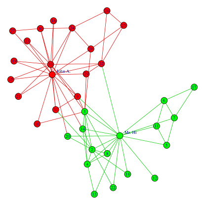
A real-world network borrowed from social science literature is here utilized for evaluating the ability to detect a community structure in a network. The chosen network is the Zachary’s karate club [16], a very well-known network that has become a benchmark test for community detection methods. This network describes the relationship of 34 members of a US university club in the 1970s. Each member is a node in the network, and a link between two nodes indicates whether two members know each other. As the time passed an internal conflict between the president, John A., and the instructor, Mr. Hi, divided the group between members that supported the president and the members that supported the instructor. The goal is to split the club members in a group that supports the president and a group that supports the instructor.

In Figure 1, the process’ result for community detection on the karate club is shown. In edges, the colors represent the class of particles that dominated the edge at the end of simulation. In vertices, the color is the result of community detection by using the density information. The color of vertices represent the community structure detected by the proposed model. Even though this is an unweighted network (the links denote only whether two members know each other) the proposed model was able to detect the correct group of members by using the weight of 1 for all links.

Figure 1: Community detection result for the proposed model on Zachary’s karate club network. Red and blue colors denote a group. For edges the color is the class of particles that dominates the edge at the end of the simulation. For vertices the color is the community to which a vertex has been grouped. All members were correctly grouped.

3.2 Simulations for the Data Clustering Problem

Six techniques with different approaches to tackle the problem of data clustering were selected to compare with the proposed technique: K-means [10], Fuzzy c-means [3], Hierarchical DBSCAN* with Density-Based Clustering Validation index (DBSCAN + DBCV) [4, 14], Chameleon [13], Expectation Maximization algorithm with parameterized Gaussian mixture models [9], and an adapted greedy algorithm based on modularity of networks [5].

In order to evaluate the quality of a partition found by an algorithm, the measure of Adjusted Rand Index [11] was calculated for each generated partition. This measure index is defined in the range $[-1,1]$ where values close to 1 indicate that the partition is close to the a prior knowledge of the dataset’s clusters and values close to zero indicate the partition is likely to be as good as an algorithm that partitions the dataset at random.

Three techniques rely on stochastic initialization (K-means, fuzzy c-means, and Expectation Maximization)—for these, the reported results are the average over 50 runs for each dataset. For the simulations all techniques had prior knowledge of the number of classes in the data clustering problem. That way, the reported results assess the ability of a technique to perform the dataset partitioning given that the number of clusters is known. In case of Chameleon and the proposed technique, the algorithms start with an possibly larger number of clusters/communities before agglomerating to the desirable number. For Chameleon, the initial number of clusters varied within $\{C,C+1,\dots,\left\lvert\mathcal{X}\right\rvert\}$, where $\left\lvert\mathcal{X}\right\rvert$ is the number of data points in the dataset. For the proposed technique, the competition parameter is fixed at $\lambda=0.5$ with the number of classes of particles varying in $\{2,5,\dots,30\}$. Moreover, modularity and the proposed technique are graph-based methods, which implies the dataset input must be in a graph representation. The k-NN method was used, varying $k\in\{1,2,\dots,30\}$.

3.2.1 Simulations on Artificial Datasets

Table 1: Adjusted Rand Index values for simulations on four artificial datasets.

	Banana	Highleyman	Lithuanian	Spirals	20cmAvg.
Rank
K-means	.2429	.2617	-.0016	-.0020	6.2
Fuzzy c-means	.2442	.3201	-.0017	-.0019	5.8
HDBSCAN + DBCV	.4714	.2085	.7024	.2507	4
Chameleon	.9215	.4348	.9343	.0119	3
Expectation Maximization	.3304	.7977	-.0015	-.0020	4.5
Modularity	.3510	.5033	.4259	1.0000	3
Proposed technique	.9408	.7164	.9538	1.0000	1.5

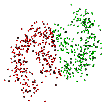
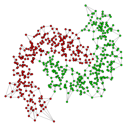
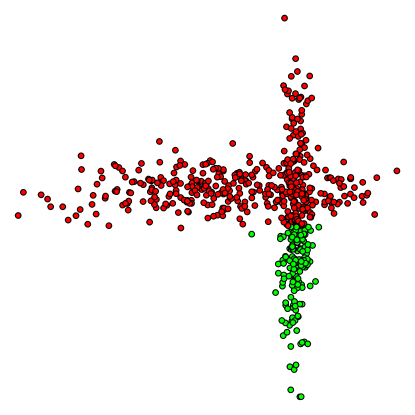
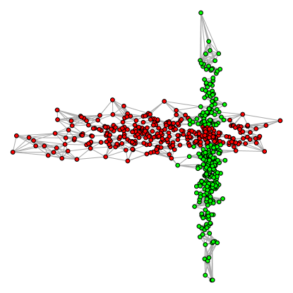
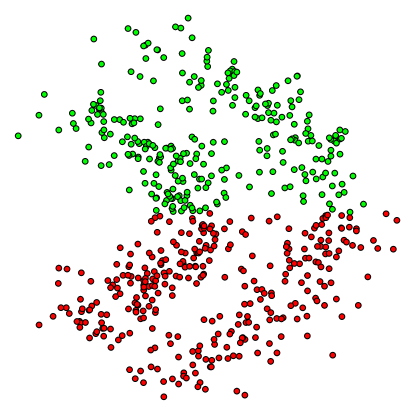
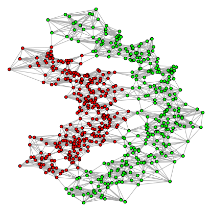
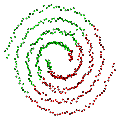
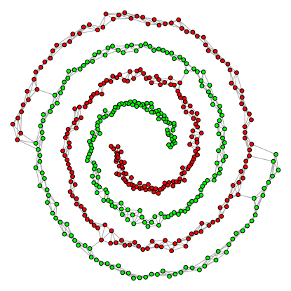
Four artificial datasets were generated with PRTools framework [7]. The datasets are formed by points in two-dimensional space equally splitted into two classes that form two clusters to be detected by the algorithm. Except for the dataset of spirals that contain 500 points, the other four datasets are formed by 600 points. Because the datasets are not in a network representation, the k-Nearest Neighbor (k-NN) graph construction method is employed to obtain a graph that is the system’s network. In the constructed network, a vertex represents a data point, and it connects to its $k$ nearest points determined by Euclidean distance.

Figures 3, 5, 3 and 5 show the generated dataset, the result obtained by application of K-means, and the result of the proposed technique. In Table 1, the adjusted rand index of each technique is shown. The last column is the average ranking position that a technique obtained. The technique is able to correctly detect the shape distribution in the four datasets. The graph representation naturally determine how particles flow through the network. If the clusters have a slow interconnectivity, as the case of spirals (see Figure 5), both modularity and the proposed, which both are network-based techniques, are able to correctly partition the data without any mistake. But the network is not the only important aspect. For instance, modularity could not partition data points of different classes in overlapping regions, as the case of Highleyman dataset, whereas the proposed was able to find a disconnected community (see Figure 3).

Figure 2: Banana-shaped distribution dataset with two classes. (a) Result obtained by K-means. (b) Result obtained by the proposed technique.

Figure 3: Highleyman dataset with two classes. (a) Result obtained by K-means. (b) Result obtained by the proposed technique.

Figure 4: Lithuanian dataset with two classes. (a) Result obtained by K-means. (b) Result obtained by the proposed technique.

Figure 5: Spirals dataset with two classes. (a) Result obtained by K-means. (b) Result obtained by the proposed technique.

3.2.2 Simulations on Real Datasets

Ten real-world datasets were selected from the UCI repository [1]. A brief description of the datasets is given in Table 2. Results of adjusted rand index for simulations of these datasets is shown in Table 3. In this table, the last column is the average ranking position of each technique over all datasets. The ranking is sorted accordingly to the adjusted rand index. A higher index indicates that a technique has partitioned the dataset in a way more similar to the prior knowledge. Thus, the technique that obtained the highest index for a dataset has a ranking position of 1 for that dataset; the second highest index is associated to a ranking position of 2, and so on.

The parameter combination the obtained the highest adjusted rand index is shown in Table 4. Notably for all real-world datasets, simulating the system with a higher value for the number $K$ of classes of particles, and thereafter in a second step merging to $C$ communities has given the best results.

Table 2: Description of the real-world datasets, with the number of data points, the number of dimensions in the attribute space, and the number of clusters the data points are partitioned.

	Instances	Dimensions	Classes
Breast cancer	699	9	2
Car evaluation	1728	6	4
Credit approval	690	15	2
Contraceptive method	1473	9	3
Glass	214	9	6
Ionosphere	351	34	2
Iris	150	4	3
Vowel	90	10	11
Wine	178	13	3
Seeds	270	7	3

Table 3: Comparison of the Adjusted Rand Index of seven different techniques on 10 real-world datasets.

20cmBreast cancer 20cmCar eval. 20cmCredit approval 20cmContr. method Glass Ion. Iris Vowel Wine Seeds 20cmAvg. Rank K-means .7302 .0294 .2389 .0215 .1610 .1776 .6540 .1736 .8582 .7049 4.8 Fuzzy c-means .7305 .0307 .3725 .0242 .1632 .1727 .7287 .0892 .8498 .7266 4.3 HDBSCAN+DBCV .2556 .1313 .0794 .0236 .2575 .7030 .5657 .0814 .3385 .4303 5.4 Chameleon .7192 .1496 .1653 .0253 .2918 .6767 .6844 .1949 .8249 .7436 3.6 E. Maximization .6955 .0367 .1987 .0112 .1571 .1547 .9222 .1541 .9472 .6671 4.8 Modularity .4474 .1872 .1734 .0329 .2118 .0708 .9038 .2505 .8858 .8125 3.5 Proposed technique .7930 .1880 .4890 .0433 .2377 .3057 .9222 .2259 .9488 .8377 1.6

Table 4: Best parameter combinations for both artificial and real-world datasets. The best combination is associated to the highest adjusted rand index obtained. The listed parameters are the k-NN, the number of classes of particles, and the order of the neighborhood considered for grouping vertices in communities.

	k-NN	$K$	Neighborhood
Banana shape	4	2	4
Lithuanian	7	24	2
Highleyman	11	8	4
Spirals	5	18	1
Breast cancer	4	30	3
Car evaluation	16	11	4
Credit approval	28	27	3
Contraceptive method	10	11	2
Glass	28	8	3
Ionosphere	9	30	2
Iris	8	5	1
Vowel	7	30	2
Wine	8	24	3
Seeds	4	21	3

It is expected that the modularity algorithm do not have a significant difference, since the intuition of the present technique is to simplify the problem by finding some communities in a first step for later optimize the partitions according to a quality function, such as the modularity. An interesting aspect of the reported results is that the average rank of presented technique do not vary much accordingly to the dataset domain, which could mean the technique does not have a great bias of domain. Nevertheless, the artificial toy datasets have a show case where the technique is able to get a better partitioning by loosing the definition of community and allowing disconnected communities.

Chameleon has a very similar insight as the proposed technique in the way it approaches the data clustering problem. First, Chameleon splits the network representation of the dataset into small groups of vertices. Afterwards, it agglomerates these groups into larger ones until obtained the desired number of clusters. One problem is the step of defining the small groups. If the small groups of vertices are not well defined—such as in cases of data with overlapping regions—, the agglomerative step will result in a poor data clustering. Conversely, if well-defined then it obtains good results as in the case of the Glass and Ionosphere datasets, which were the two datasets the Chameleon obtained a higher value for adjusted rand index.

Figure 6: Visualization of post-hoc Bonferroni–Dunn test. Fixing the proposed technique as the control, the average ranking of the other six techniques were compared. All techniques with average rankings outside the bold-marked interval are significantly different from the proposed technique, with a significance level of $5\%$.

In order to evaluate whether the average ranking position of the techniques are significantly different, the average rankings are examined in a statistical manner. The methodology applied here follows a procedure described in [6, 12]. The first test, Friedman test compares the techniques under the null-hypothesis that all the techniques are equivalent and so their average rank positions. According to [6], since we have $N=10$ datasets and $k=7$ techniques, we have the degrees of freedom $\text{df1}=k-1=6$ and $\text{df2}=(N-1)(k-1)=54$, resulting in the critical value $F(6,54)\approx 2.27$. With such values, we get a Friedman statistic $F_{F}\approx 4.88$. Since $F_{F}>F(6,54)$ the null-hypothesis is rejected at a $5\%$ significance level, allowing us to proceed with a post-hoc test.

Fix a significance level of $5\%$ for the post-hoc. The interest is at comparing the proposed model with the other six techniques. For that the Bonferroni–Dunn test is employed, because there are multiple techniques over multiple datasets, and only the difference between a fixed technique and all others is of interest [12]. Therefor, six null-hypothesis of the proposed technique’s average rank being equivalent to an other technique are tested. To accomplish this, the $t$ statistic between a fixed and an other technique must be by at least a Critical Difference (CD). If they differ that much, then the null-hypothesis is rejected and therefore there is a significant statistical difference between the average ranking position of the two techniques. For the setting in this paper, we get a $\text{CD}\approx 3.33$. The proposed technique has significant statistical difference when compare with K-means, Fuzzy c-means, HDBSCAN + DBCV, and Expectation Maximization. The techniques Chameleon and Modularity do not present significant statistical difference. But, nevertheless, these two together with the proposed technique, put network-based methods in a good position at data clustering problems. A visualization of the post-hoc test, as suggested in [6], is shown in Figure 6.

4 Conclusion

In this paper, a novel model for particle competition in complex networks is presented. Particles flow through the network and their presence dominates an edge. The information is then used to determine the pertinence of vertices in communities of the network. A second step allows the maximization of the modularity by locally maximizing the modularity of the community structure. This final structure is used to the problem of data clustering.

Simulations on both artificial and real-world datasets show that the proposed technique performs well and have a significant better performance under the condition that the algorithms have prior knowledge of the number of clusters. Furthermore, the technique has a deterministic alternative model with a low computational complexity.

The information of dominance of edges have a potentially higher granularity information about the interaction network formed by the graph representation of the dataset. This information might allow to grasp more properties of the process and consequently help into find a better approach to the local maximization of the community structure.

Finally, in a data clustering setting it is not uncommon to run algorithms on datasets with noise and no prior knowledge of the number of clusters. The proposed technique here present could be extended for such applications.

References

- [1] D J Newman A. Asuncion “UCI Machine Learning Repository”, 2007
- [2] Alain Barrat, Marc Barthlemy and Alessandro Vespignani “Dynamical Processes on Complex Networks” New York, NY, USA: Cambridge University Press, 2008
- [3] James C. Bezdek, Robert Ehrlich and William Full “FCM: The fuzzy c-means clustering algorithm” In Computers & Geosciences 10.2–3, 1984, pp. 191–203 DOI: 10.1016/0098-3004(84)90020-7
- [4] Rjgb Campello, Davoud Moulavi and Joerg Sander “Density-based clustering based on hierarchical density estimates” In Advances in Knowledge Discovery …, 2013, pp. 160–172
- [5] Aaron Clauset, M. J Newman and Cristopher Moore “Finding community structure in very large networks” In Physical Review E - Statistical, Nonlinear, and Soft Matter Physics 70.6 2, 2004, pp. 1–6 DOI: 10.1103/PhysRevE.70.066111
- [6] Janez Dems̆ar “Statistical Comparisons of Classifiers over Multiple Data Sets” In J. Mach. Learn. Res. 7, 2006, pp. 1–30
- [7] R.P.W. Duin et al. “PR-Tools4.1, A Matlab Toolbox for Pattern Recognition” Delft University of Technology, 2007
- [8] Santo Fortunato “Community detection in graphs” In Physics Reports 486.3-5, 2010, pp. 75–174 DOI: 10.1016/j.physrep.2009.11.002
- [9] Chris Fraley, Adrian E Raftery, T Brendan Murphy and Luca Scrucca “mclust Version 4 for R : Normal Mixture Modeling for Model-Based Clustering , Classification , and Density Estimation” In Technical Report 597, University of Washington, 2012
- [10] J.. Hartigan and M.. Wong “A K-Means Clustering Algorithm” In Journal of the Royal Statistical Society 28.1, 1979, pp. 100–108
- [11] Lawrence Hubert and Phipps Arabie “Comparing partitions” In Journal of Classification 2.1, 1985, pp. 193–218 DOI: 10.1007/BF01908075
- [12] Nathalie Japkowicz and Mohak Shah “Evaluating Learning Algorithms: A Classification Perspective”, 2011, pp. 423 DOI: http://dx.doi.org/10.1017/CBO9780511921803
- [13] George Karypis, Eui-Hong Han and Vipin Kumar “Chameleon: hierarchical clustering using dynamic modeling” In Computer 32.8, 1999, pp. 68–75 DOI: 10.1109/2.781637
- [14] Davoud Moulavi, Pa Jaskowiak and Rjgb Campello “Density-Based Clustering Validation” In Dbs.Ifi.Lmu.De, 2014
- [15] M… Newman “Fast algorithm for detecting community structure in networks” In Physical Review E 69.6, 2004, pp. 066133 DOI: 10.1103/PhysRevE.69.066133
- [16] W Zachary “An Information Flow Model for Conflict and Information Fission in Small Groups” In Journal of anthropological research 33.4, 1977, pp. 452–473 DOI: 10.2307/3629752