Pairing and deformation effects in nuclear excitation spectra

Abstract

We investigate effects of pairing and of quadrupole deformation on two sorts of nuclear excitations, $\gamma$-vibrational $K^{\pi}=2^{+}$ states and dipole resonances (isovector dipole, pygmy, compression, toroidal). The analysis is performed within the quasiparticle random-phase approximation (QRPA) based on the Skyrme energy functional using the Skyrme parametrization SLy6. Particular attention is paid to i) the role of the particle-particle (pp) channel in the residual interaction of QRPA, ii) comparison of volume pairing (VP) and surface pairing (SP), iii) peculiarities of deformation splitting in the various resonances. We find that the impact of the pp-channel on the considered excitations is negligible. This conclusion applies also to any other excitation except for the $K^{\pi}=0^{+}$ states. Furthermore, the difference between VP and SP is found small (with exception of peak height in the toroidal mode). In the low-energy isovector dipole (pygmy) and isoscalar toroidal modes, the branch $K^{\pi}=1^{-}$ is shown to dominate over $K^{\pi}=0^{-}$ one in the range of excitation energy $E<$ 8–10 MeV. The effect becomes impressive for the toroidal resonance whose low-energy part is concentrated in a high peak of almost pure $K^{\pi}=1^{-}$ nature. This peculiarity may be used as a fingerprint of the toroidal mode in future experiments. The interplay between pygmy, toroidal and compression resonances is discussed, the interpretation of the observed isoscalar giant dipole resonance is partly revised.

I Introduction

Pairing is known to play an important role in low-energy nuclear excitations SSS ; Ri80 . For the ground state, it is usually treated within the Bardeen-Cooper-Shrieffer (BCS) scheme or Hartree-Fock-Bogoliubov (HFB) method, see e.g. SSS ; Ri80 ; Do84 ; Do96 ; Re97 ; Be00 ; Ta04 . Nuclear excitations are described with the Quasiparticle Random Phase Approximation (QRPA) where the pairing-induced particle-particle (pp) channel is added to the particle-hole (ph) residual interaction SSS ; Ri80 ; Te05 ; Li08 . During last decades, both static and dynamical pairing aspects were thoroughly explored in schematic and self-consistent models, see e.g. SSS ; Do84 ; Do96 ; Re97 ; Be00 ; Ta04 ; Te05 ; Li08 ; Iud05 ; Se08 ; Te10 ; Te11g . The pp-channel was found important in electric modes with positive parity (monopole, quadrupole) where it generates pairing vibrations, see e.g. SSS ; Ri80 ; Li08 ; Iud05 . In deformed axial nuclei, the pp-channel is important in states with $K^{\pi}=0^{+}$ where $K$ is the projection of the angular momentum SSS ; Iud05 ; Te10 ; Te11g .

In spite of extensive studies, some pairing effects in nuclear excitations still deserve further exploration, especially in deformed nuclei. For example, it is yet unclear if we indeed need the pp-channel in the self-consistent description of excitations with $K^{\pi}\neq 0^{+}$. These excitations include all negative-parity states (dipole, octupole, …) as well as positive-parity states with $K>0$. Clarification of this point is important because the pp-channel considerably complicates QRPA calculations. A further point of interest is to check the influence of surface pairing (SP) as compared to volume pairing (VP).

These two problems are addressed in the present study for the case of the standard monopole $\delta$-force pairing. The calculations are performed within the self-consistent QRPA method Re16 with the Skyrme force SLy6 Cha97 . As typical examples we consider ^152,154,156Sm which are well deformed having still axially symmetric shape. In a first step, we inspect the lowest $\gamma$-vibrational states with $K^{\pi}=2^{+}$. The previous systematic self-consistent explorations of $\gamma$-vibrational states were performed with Te11g and without Ne16g the pp-channel. We will show that the effect of pp-channel is very small in these modes. At least it is much weaker than the difference between the results obtained with VP and SP.

In a second step, we inspect exotic parts of the dipole excitation spectrum which attract high attention presently (see, e.g., Pa07 ; Kv11 ; Re13 ), namely low-lying isovector strength also coined pygmy dipole resonance (PDR), toroidal dipole resonance (TDR), and compression dipole resonance (CDR). These modes are located, fully or partly, at rather low energies and so may be affected by pairing. Here again we have found the pp-channel negligible. Altogether, our analysis suggests that the pp-channel can be ignored in QRPA calculations for all excitations with $K^{\pi}\neq 0^{+}$.

The next point of our study concerns deformation effects in dipole excitations. We analyze the ordinary isovector giant dipole resonance (GDR), PDR, and isoscalar TDR and CDR. The TDR and CDR are often considered as low- and high-energy parts of the isoscalar giant dipole resonance (ISGDR) Pa07 ; Har . In axial nuclei, all these resonances exhibit a deformation splitting into $K=0$ and $K=1$ branches. However, the features of these branches depend very much on the actual type of resonance. For example, our previous studies have shown that the main low-energy peak of the TDR is, somewhat surprisingly, dominated by $K=1$ strength instead of $K=0$ one as would have expected Kv13Sm ; Kv14Yb ; Ne17 . In fact, the TDR produces the opposite sequence of $K$-branches as compared to the GDR. Since the TDR shares the same energy region as the PDR and is, in fact, the source of the PDR Re13 , this anomaly becomes especially interesting because it can be related to the deformation splitting of the PDR. In this connection, we propose here a further comparative analysis of the deformation splitting of various dipole modes with the main accent to the low-energy region embracing PDR and TDR.

The paper is organized as follows. In Sec. 2, the calculation scheme is outlined paying particular attention to the treatment of pairing. The main factors determining the impact of the pp-channel are discussed comparing analytically the pp- and ph-channels. In Sec. 3, results of the QRPA calculations for $K^{\pi}=2^{+}$ states and dipole modes are presented and discussed. Some experimental perspectives are commented. In Sec. 4, conclusions are given. In Appendix A, the Skyrme functional used in this paper is sketched. In Appendix B, the actual HF+BCS scheme is outlined. In Appendix C, the basic QRPA equations with pp-channel are presented.

II Calculation scheme and theoretical background

II.1 Method and numerical details

The calculations are performed within QRPA Ri80 based on the Skyrme energy functional Skyrme ; Vau ; Be03

$$\mathcal{E}(\rho,\tau,{\bf J},\vec{j},\vec{s},\vec{T},\tilde{\rho})=\mathcal{E}_{\rm kin}+\mathcal{E}_{\rm Sk}+\mathcal{E}_{\rm Coul}+\mathcal{E}_{\rm pair}$$ (1)

including kinetic, Skyrme, Coulomb and pairing parts. The Skyrme part $\mathcal{E}_{\rm{Sk}}$ depends on the following local densities and currents: density $\rho(\vec{r})$, kinetic-energy density $\tau(\vec{r})$, spin-orbit density $\mathbf{J}(\vec{r})$, current $\vec{j}(\vec{r})$, spin density $\vec{s}(\vec{r})$, and spin kinetic-energy density $\vec{T}(\vec{r})$. The Coulomb exchange term is treated in Slater approximation. The pairing functional is derived from monopole contact $\delta$-force interaction Be00 . This functional depends on the pairing density $\tilde{\rho}(\mathbf{r})$ and, for the surface pairing, also on the normal density $\rho(\mathbf{r})$. More details on the functional (1) can be found in the next subsection and in Appendix A.

The mean-field Hamiltonian and the QRPA residual interaction are determined through the first and second functional derivatives of the total energy (1). The approach is fully self-consistent since: i) both the mean field and residual interaction are obtained from the same Skyrme functional, ii) time-even and time-odd densities are involved, iii) the residual interaction includes all the terms of the initial Skyrme functional as well as the Coulomb direct and exchange terms, iv) both ph- and pp-channels in the residual interaction are taken into account. Details of our mean field and QRPA schemes are given in Appendices B and C. The present version of the Skyrme QRPA scheme is implemented in the two-dimensional (2D) QRPA code Re16 .

The calculations are performed with the Skyrme force SLy6 Cha97 which was successfully used earlier for a systematic exploration of the GDR in rare-earth, actinide and superheavy nuclei Kl08 . The QRPA code employs a 2D mesh in cylindrical coordinates. The calculation box extends over three times the nuclear radius. The mesh size is 0.4 fm. The single-particle spectrum taken into account embraces all levels from the bottom of the potential well up to +30 MeV. The (axial) equilibrium quadrupole deformation is determined by minimization of the total nuclear energy. This yields the deformation parameters $\beta$ = 0.311, 0.339, and 0.361 for ^152,154,156Sm, respectively, which are sufficiently close to the experimental values $\beta_{\rm exp}$ = 0.308 for ¹⁵²Sm and $\beta_{\rm exp}$ = 0.339 for ¹⁵⁴Sm bnl_exp .

Pairing in the ground state is treated with the HF+BCS scheme, see next subsection. To cope with the principle divergency of short-range forces, we implement in the HF+BCS equations and pairing transition densities a soft, energy-dependent cutoff factor Be00

$$f^{q}_{i}=\frac{1}{1+\exp\Big{[}\frac{e^{q}_{i}-\lambda_{q}-\Delta E_{q}}{\eta_{q}}\Big{]}}$$ (2)

where $q=\{n,p\}$, $i$ denotes single-particle states, $e^{q}_{i}$ is the single-particle energy, and $\lambda_{q}$ is the chemical potential. The cutoff parameter $\Delta E_{q}$ and width $\eta_{q}=\Delta E_{q}/10$ are chosen self-adjusting to the actual level density in the vicinity of the Fermi energy Be00 . Here $\Delta E_{q}$ lies around 6 MeV. In the pp-channel, two-quasiparticle (2qp) states $(i,j)$ are limited to those with $\sqrt{f^{q}_{i}f^{q}_{j}}>10^{-4}$ to remove high-energy particle states. More information on the pairing formalism is given in the next subsection.

To minimize the calculational expense in ph-channel, we employ only states with $|u_{i}v_{j}+v_{i}u_{j}|>10^{-4}$, where $u_{i},v_{i}$ are coefficients of the special Bogoliubov transformation. This cut-off still leaves the 2qp configuration space large enough to exhaust the energy-weighted sum rules (EWSR). Note also that a large configuration space in ph-channel is crucial for a successful description of low-energy vibrational excitations Ne16g and extraction of the spurious admixtures Re16 ; Rei92d . For example, in calculations of $\gamma$-vibrational modes in ¹⁵⁴Sm, we deal with $\approx 6300$ proton and $\approx 12500$ neutron pairs and exhaust the isoscalar quadrupole $\mathrm{EWSR}=(\hbar e)^{2}/(8\pi m)\cdot 50A\langle r^{2}\rangle_{A}$ by $\approx$ 97 $\%$. The Thomas-Reiche-Kuhn sum rule for dipole excitations is exhausted in the interval 2–45 MeV by $\approx$ 94 $\%$.

II.2 Treatment of pairing

The pairing part in the functional (C.1) reads

$$\mathcal{E}_{\rm pair}=\frac{1}{4}\>\sum_{q=n,p}V_{q}\>\int\mathrm{d}\vec{r}\>|\tilde{\rho}_{q}(\vec{r})|^{2}\>G_{q}(\vec{r})\;.$$ (3)

It is motivated by the zero-range pairing interaction Be00

$$V^{q}_{\rm pair}(\vec{r},\vec{r}^{\prime})=G_{q}(\vec{r})\delta(\vec{r}-\vec{r}^{\prime})$$ (4)

with

$$G_{q}(\vec{r})=V_{q}\Big{[}1-\eta\>\Big{(}\frac{\rho(\vec{r})}{\rho_{0}}\Big{)}^{\!\gamma}\Big{]}.$$ (5)

Here $\rho(\vec{r})=\rho_{p}(\vec{r})+\rho_{n}(\vec{r})$ is the sum of normal proton and neutron densities, $\tilde{\rho}_{q}(\vec{r})$ are the pairing densities, $V_{q}$ are pairing strength constants, and $\rho_{0}$=0.16 ${\rm fm}^{-1}$ is the saturation density of symmetric nuclear matter. The coefficient $\gamma$ regulates the density dependence. Following common practice, we fix here $\gamma$=1. We obtain so-called volume pairing (VP) for $\eta$=0 and the (density-dependent) surface pairing (SP) for $\eta$=1. Of course, $\eta$ may be varied freely and take values in between 0 and 1, when optimized properly Klu09a . We consider here VP and SP as limiting cases to explore the sensitivity to the pairing model.

Pairing is treated within the HF+BCS scheme described in Appendix B. In this scheme, the nucleon and pairing densities in axial nuclei read Be03

$$\rho_{q}(\vec{r}) = 2\sum_{i\epsilon q}v_{i}^{2}|\psi_{i}(\vec{r})|^{2},$$ (6)

$$\tilde{\rho}_{q}(\vec{r}) = -2\sum_{i\epsilon q}f_{i}^{q}v_{i}u_{i}|\psi_{i}(\vec{r})|^{2}$$ (7)

where $\psi_{i}(\vec{r})$ are single-particle wave functions and $f^{q}_{i}$ is the energy-dependent cut-off weight (2).

Pairing induces the pp-channel in the QRPA residual interaction, see Appendix C. Its contributions to the QRPA matrices A and B are given by expressions (C.4)-(C.6). For $\gamma$=1, these contributions read:

$$A^{\rm pair}_{qq^{\prime}}(i{\bar{j}},i^{\prime}{\bar{j}}^{\prime}) = \frac{1}{2}\delta_{qq^{\prime}}V_{q}\int\mathrm{d}\vec{r}\Big{[}1-\eta\frac{\rho({\vec{r}})}{\rho_{0}}\Big{]}\delta\tilde{\rho}^{q}_{i{\bar{j}}}(\vec{r})\delta\tilde{\rho}^{q^{\prime}}_{i^{\prime}{\bar{j}}^{\prime}}(\vec{r})$$ (8)

$$- \frac{\eta}{2\rho_{0}}V_{q}\int\mathrm{d}\vec{r}\tilde{\rho}_{q}(\vec{r})\delta\tilde{\rho}^{q}_{i\bar{j}}(\vec{r})\delta{\rho}^{q^{\prime}}_{i^{\prime}\bar{j}^{\prime}}(\vec{r})$$

$$- \frac{\eta}{2\rho_{0}}V_{q^{\prime}}\int\mathrm{d}\vec{r}\tilde{\rho}_{q^{\prime}}(\vec{r})\delta\rho^{q}_{i\bar{j}}(\vec{r})\delta\tilde{\rho}^{q^{\prime}}_{i^{\prime}\bar{j}^{\prime}}(\vec{r})$$

with

$$B^{\rm pair}_{i{\bar{j}}i^{\prime}{\bar{j}}^{\prime}}=-A^{\rm pair}_{i{\bar{j}}\>i^{\prime}{\bar{j}}^{\prime}}.$$ (9)

Here we assume that $i{\bar{j}}\in q,\>i^{\prime}{\bar{j}}^{\prime}\in q^{\prime}$. Furthermore

$$\delta\rho^{q}_{i{\bar{j}}}(\vec{r})=(u_{i}v_{j}+u_{j}v_{i})\psi^{*}_{i}(\vec{r})\psi_{j}(\vec{r})$$ (10)

$$\delta\tilde{\rho}^{q}_{i{\bar{j}}}(\vec{r})=\sqrt{f^{q}_{i}f^{q}_{j}}\>(u_{i}u_{j}-v_{j}v_{i})\psi^{*}_{i}(\vec{r})\psi_{j}(\vec{r})$$ (11)

are 2qp nucleon and pairing transition densities.

The contributions (8)-(9) constitute the pairing-induced pp-channel. The first term in (8) exists for both VP and SP. It is diagonal in $q$ since we do not consider a proton-neutron pairing. The next two terms which mix nucleon and pairing density are caused by the density-dependence of SP and so exist only in SP case. In the present study we consider only quadrupole states $K^{\pi}=2^{+}$ and dipole states. Then the transition densities (10) and (11) include only non-diagonal 2qp configurations with $i\neq j$.

It is instructive to compare the contributions to QRPA matrices from ph- and pp-channels. The ph-contribution to the A-matrix from the Skyrme functional is dominated by Ne06

$$\frac{\delta\mathcal{E}_{\rm Sk}}{\delta\rho^{q}\delta\rho^{q^{\prime}}}=b_{0}-b_{0}^{\prime}\delta_{qq^{\prime}}$$ (12)

where $b_{0}$ and $b_{0}^{\prime}$ are coefficients of the Skyrme interaction given in the Appendix A. This results in

$$A^{\rm ph}_{qq^{\prime}}(i{\bar{j}},i^{\prime}{\bar{j}}^{\prime})=(b_{0}-b_{0}^{\prime}\delta_{qq^{\prime}})\int d\vec{r}\delta\rho^{q}_{i{\bar{j}}}(\vec{r})\delta\rho^{q^{\prime}}_{i^{\prime}{\bar{j}}^{\prime}}(\vec{r})$$ (13)

to be compared for $q=q^{\prime}$ with the pp-contribution (8). For states $i$ and $j$ near the Fermi level, the transition densities (10) and (11) are of the same order of magnitude. Then the ratio between ph and pp contributions is mainly determined by the ratio of the channel strengths

$$R_{q}=\frac{2(b_{0}-b_{0}^{\prime})}{V_{q}}.$$ (14)

For SLy6, $b_{0}=-3502.3$ MeV, $b_{0}^{\prime}=-3285.3$ MeV. Further, $V_{p}=-298.8$ MeV fm³, $V_{n}=-288.5$ MeV fm³ for VP and $V_{p}=-1053.12$ MeV fm³, $V_{n}=-864.2$ MeV fm³ for SP Fle04 . Then the ratios are $R_{n}=1.50$, $R_{p}=1.45$ for VP and $R_{n}=0.50$, $R_{p}=0.41$ for SP. In average, $R_{q}\sim 1$, i.e. Skyrme amplitudes in ph-channel and pairing amplitudes in pp-channel are similar (though, for SP, one may expect somewhat larger effect of pp-channel than for VP).

The observations that $\rho^{q}_{ij}\sim\tilde{\rho}^{q}_{ij}$ and $R_{q}\sim$1 do not yet suffice to conclude that ph- and pp-channels are of the same order of magnitude. We should also take into account that in ph-channel the main interaction is the proton-neutron one (with the amplitude $b_{0}$). This interaction is much stronger than its proton-proton and neutron-neutron counterparts characterized by the amplitudes $b_{0}-b_{0}^{\prime}$. Indeed, for SLy6, $b_{0}/(b_{0}-b_{0}^{\prime})=16.1$. Pairing, on the other hand, has no neutron-proton interaction at all. Besides, in the pairing pp-channel, the contribution of 2qp configurations with high-energy states is suppressed by the cut-off (2). So in general one may expect that the ph-channel is much stronger than the pp-channel.

Note that the above qualitative analysis mainly concerns states with $K^{\pi}\neq 0^{+}$. For $K^{\pi}=0^{+}$ states, the situation becomes much more complicated. Here the diagonal 2qp configurations $i\bar{i}$, resulting in the pairing vibrations, come into play. Thus the pp-channel, even being still weaker than its ph-counterpart, becomes important for low-energy excitations SSS ; Ri80 .

II.3 QRPA strength functions

The energy-weighted strength function for electric transitions of multipolarity $\lambda\mu$ between QRPA ground state $|{\rm gr}\rangle$ and excited state $|\nu\rangle$ has the form

$$S_{X}(E\lambda\mu,T;E)=\sum_{\nu}E_{\nu}\>\big{|}\langle\nu|\>\hat{M}^{X}_{\lambda\mu}(T)\>|{\rm gr}\rangle\big{|}^{2}\>\xi_{\Delta}(E-E_{\nu})$$ (15)

where $E$ is the excitation energy, $\hat{M}^{X}_{\lambda\mu}(T)$ is the transition operator, $X=\{\rm el,com,tor\}$ marks the type of the excitation (isovector E1(T=1), compression isoscalar E1(T=0), toroidal isoscalar E1(T=0)), $E_{\nu}$ is the energy of the QRPA state. For excited states $K^{\pi}_{\nu}$, we assume $K=\mu$, $\pi=(-1)^{\lambda}$. The total strength functions read

$$S_{X}(E\lambda,T;E)=\sum_{\mu\geq 0}(2-\delta_{\mu,0})S_{X}(E\lambda\mu,T;E).$$ (16)

The strengths are weighted by the Lorentz function

$$\xi_{\Delta}(E-E_{\nu})=\frac{1}{2\pi}\frac{\Delta(E)}{(E-E_{\nu})^{2}+[\Delta(E)/2]^{2}}$$ (17)

with the energy-dependent folding Kv13Sm

$$\Delta(E)=\left\{\begin{array}[]{ll}\Delta_{0}&\>{\rm for}\>\>\>E\leq E_{0},\\ \Delta_{0}+a\>(E-E_{0})&\>{\rm for}\>\>\>E>E_{0}.\end{array}\right.$$ (18)

The weight $\xi_{\Delta}(E-E_{\nu})$ is used to simulate escape width and coupling to the complex configurations. Since these two effects grow with increasing the excitation energy, we employ an energy dependent folding width $\Delta(E)$. The parameters $\Delta_{0}$=0.1 MeV, $E_{0}$=8.3 MeV and $a=$0.45 are chosen so as to reproduce the smoothness of the experimental photoabsorprion in ¹⁵⁴Sm. The value $E_{0}$ roughly corresponds to the neutron and proton separation energies in ¹⁵⁴Sm: $S_{n}$=8.0 MeV and $S_{p}$=9.1 MeV bnl_exp .

The operator for the electric $E1\mu(T=1)$ transition reads

$$\hat{M}^{el}_{1\mu}(T=1)=e\sum_{i=1}^{A}e^{\rm eff}_{i}\>r_{i}Y_{1\mu}(\Omega_{i})$$ (19)

where $Y_{1\mu}(\Omega_{i})$ is the spherical harmonic and $e^{\rm eff}_{i}$ are effective charges equal to $N/A$ for protons and $-Z/A$ for neutrons. The operators for the compression and toroidal $E1\mu(T=0)$ transitions are Kv11

$$\hat{M}^{\rm com}_{1\mu}(T=0)=\frac{e}{10}\>\sum_{i=1}^{A}[r_{i}^{3}-\frac{5}{3}\langle r^{2}\rangle_{0}r_{i}]Y_{1\mu}(\Omega_{i}),$$ (20)

$$\hat{M}^{\rm tor}_{1\mu}(T=0)=-\frac{1}{2c\sqrt{3}}\int d\vec{r}\>\hat{{\bf j}}_{\rm nuc}(\vec{r}-\vec{r}_{i})$$

$$\cdot\big{[}\frac{\sqrt{2}}{5}r^{2}_{i}{\bf Y}_{12\mu}(\Omega_{i})+(r^{2}_{i}-\langle r^{2}\rangle_{0}){\bf Y}_{10\mu}(\Omega_{i})\big{]}$$ (21)

where ${\bf Y}_{10\mu}(\Omega_{i})$, ${\bf Y}_{12\mu}(\Omega_{i})$ are vector spherical harmonics; $\hat{\vec{j}}_{\rm nuc}(\vec{r}-\vec{r}_{i})=-ie\hbar/(2m)\sum_{i=1}^{A}[\delta(\vec{r}-\vec{r}_{i})\vec{\nabla}_{i}+\vec{\nabla}_{i}\delta(\vec{r}-\vec{r}_{i})]$ is operator of the isoscalar convection nuclear current. The terms with the squared ground-state radius $\langle r^{2}\rangle_{0}$ represent the center-of-mass-corrections. Note that the compression operator (20) is also the transition (probe) operator for ISGDR Har .

The photoabsorption Ri80 is related to the strength function (16) as

$$\sigma(E)\>[{\rm fm}^{2}]\>\approx 0.402\>S_{\rm el}(E1,T=1;\>E).$$ (22)

III Results and discussion

III.1 $\gamma$-vibrational states

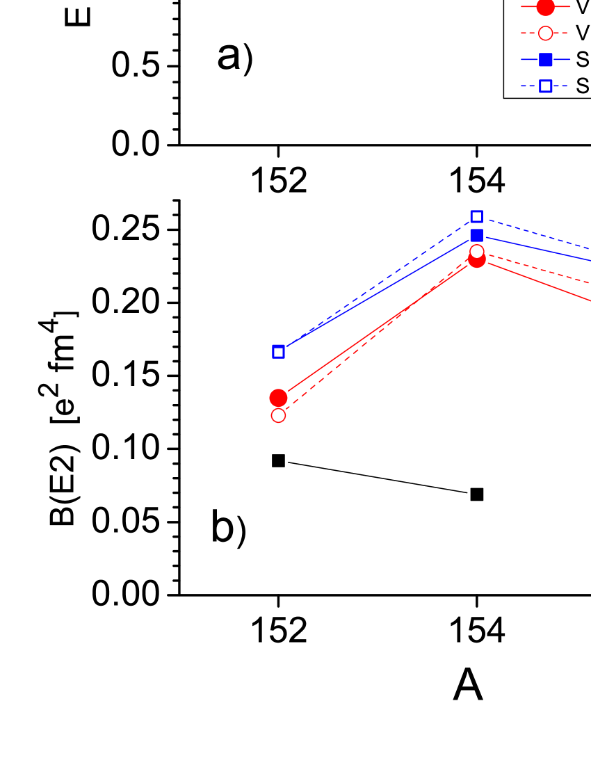
Figure 1: Energies (upper panel) and B(E2) values (lower panel) for the lowest gamma-vibrational states $K^{\pi}_{i}=2^{+}_{1}$ in ^152,154,156Sm, calculated with (full symbols) and without (open symbols) the pp-channel. Both cases of volume (VP) and surface (SP) pairing are considered. The experimental data are taken from bnl_exp .

Figs. 1-4 collect results of our calculations for $\gamma$-vibrational states in ^152,154,156Sm. Fig. 1 shows energies and $B(E2;\>gr\rightarrow I^{\pi}K=2^{+}2)$ values computed with and without the pp-channel for VP and SP cases. The reduced transition probabilities are obtained with the effective charges $e^{\rm eff}=1$ for protons and $e^{\rm eff}=0$ for neutrons. Fig. 1 indicates that the present QRPA description is not fully satisfying: the calculations essentially overestimate the experimental energies in ^152,154Sm and $B(E2)$ in ¹⁵⁴Sm. Note that such significant overestimation of energies of $\gamma$-vibrational states in ^152,154Sm has been already observed in previous self-consistent Skyrme QRPA calculations Te11g ; Ne16g . It was shown Ne16g that this problem can be partly solved by taking into account the pairing blocking effect and using a more appropriate Skyrme parametrization. Besides that, the coupling with complex (two-phonon) configurations could be here important SSS .

Figure 2: Nucleon (left) and pairing (right) proton and neutron QRPA transition densities for the lowest gamma-vibrational $K^{\pi}_{i}=2^{+}_{1}$ -state in ¹⁵⁴Sm, calculated with VP. The densities are plotted in the x-z plane for $x,z\geq 0$. The filled (open) circles represent positive (negative) values. Magnitudes of the densities are depicted by the circle size (in arbitrary units). The nuclear surface is marked by the solid line.

As seen from Fig. 1, VP and SP results are rather similar though VP performance is somewhat better. What is remarkable, for both VP and SP, the impact of the pp-channel is very small, which actually means that the pp-channel is much weaker than the ph-one (at least its impact is much smaller than the difference between VP and SP results).

This conclusion can also be drawn from Fig. 2 which shows the pairing and nucleon transition densities (TD) for the $\gamma$-vibrational state ($\lambda\mu\nu$ = 221) in ¹⁵⁴Sm, using VP. We see that, at the nuclear surface, nucleon TD $\delta\rho^{q}_{221}$ are much larger than pairing TD $\delta\tilde{\rho}^{q}_{221}$, especially for neutrons. The same takes place in Fig. 3 for the case of SP.

The next question is: what is the origin of the difference in the nucleon and pairing one-phonon TD? To clarify this point, we should numerically analyze the main ingredients of the contributions (8)–(9) of the pp-channel to the RPA matrices. First of all, let’s consider nucleon (10) and pairing (11) TD for the main 2qp component of the $\gamma$-vibrational state. This is the proton $F,F+3$ configuration $pp[413\downarrow-411\downarrow]$ (here we use asymptotic Nilsson quantum numbers, $F$ denotes the Fermi level). The TD for this configuration are shown in Fig. 4 for the case of VP. It is seen that the nucleon and pairing TD are very similar. This is not surprising since both TD have the same coordinate dependence and deviate only by the pairing factors which are of the same order of magnitude for the states near the Fermi level. As shown in Sec. II.2, the strength coefficients of the pp- and ph-channels are also similar. So indeed, following the discussion in Sec. II.2, the weakness of the pp-channel is perhaps mainly caused by the absence of the neutron-proton interaction (which plays a dominant role in ph-channel).

Figure 3: The same as in Fig. 2 but for SP.

Figure 4: Nucleon TD (10) and pairing TD (11) for the lowest 2qp proton excitation $ij=pp[413\downarrow-411\downarrow]$ in ¹⁵⁴Sm, calculated for VP. See caption to Fig. 2 for more details.

The conclusion that the pp-channel plays a negligible role can, in principle, be generalized to arbitrary states with $K^{\pi}\neq 0^{+}$ in even-even nuclei, e.g. to all states of negative parity. This allows to ignore the pp-channel from the onset and thus considerably decrease the numerical expense of QRPA.

III.2 Dipole excitations

The previous subsection concluded that pp-channel has negligible impact for low-energy $K^{\pi}\neq 0^{+}$ states. This should be even more the case for excitations with higher energies, e.g. for the various dipole resonances. For these modes, the pairing gap $\Delta_{q}\sim$ 2 MeV is much smaller than the resonance energies and so the impact of pairing should be even weaker than for low-energy excitations. Note that low-energy excitations are composed from 2qp pairs whose single-particle states $\{i,j\}$ are placed near the Fermi level and so are strongly affected by pairing. Instead, in high-energy excitations, at most one single-particle state from the 2qp pair can originate from the Fermi level region. Thus in general high-energy 2qp excitations are much less affected by pairing than low-energy ones and so, in principle, should be only weakly affected by the pairing-induced pp-channel. For the same reason, the difference between VP and SP in the resonance region is also expected to be negligible. This will be confirmed below by our QRPA calculations for GDR, PDR, TDR and CDR in ¹⁵⁴Sm. In this subsection, we will consider peculiarities of the deformation splitting of the dipole resonances in this nucleus. The main attention will be paid to a comparison of their $K=0$ and $K=1$ branches in the low-lying energy interval 3–9 MeV, embracing PDR and TDR. In what follows, it is assumed that $K=1$ branch includes both $K=\pm$1 contributions.

Use of a large configuration space allows to keep the spurious center-of-mass mode at low energies $<2$ MeV. The elimination of this mode from the dipole strength functions is additionally ensured by using appropriate effective charges and correction terms, see Sec. 2.3. In the following, we discuss dipole strength functions only for the excitation energy $E>$ 3 MeV, which is at the safe side with respect to the center-of-mass mode.

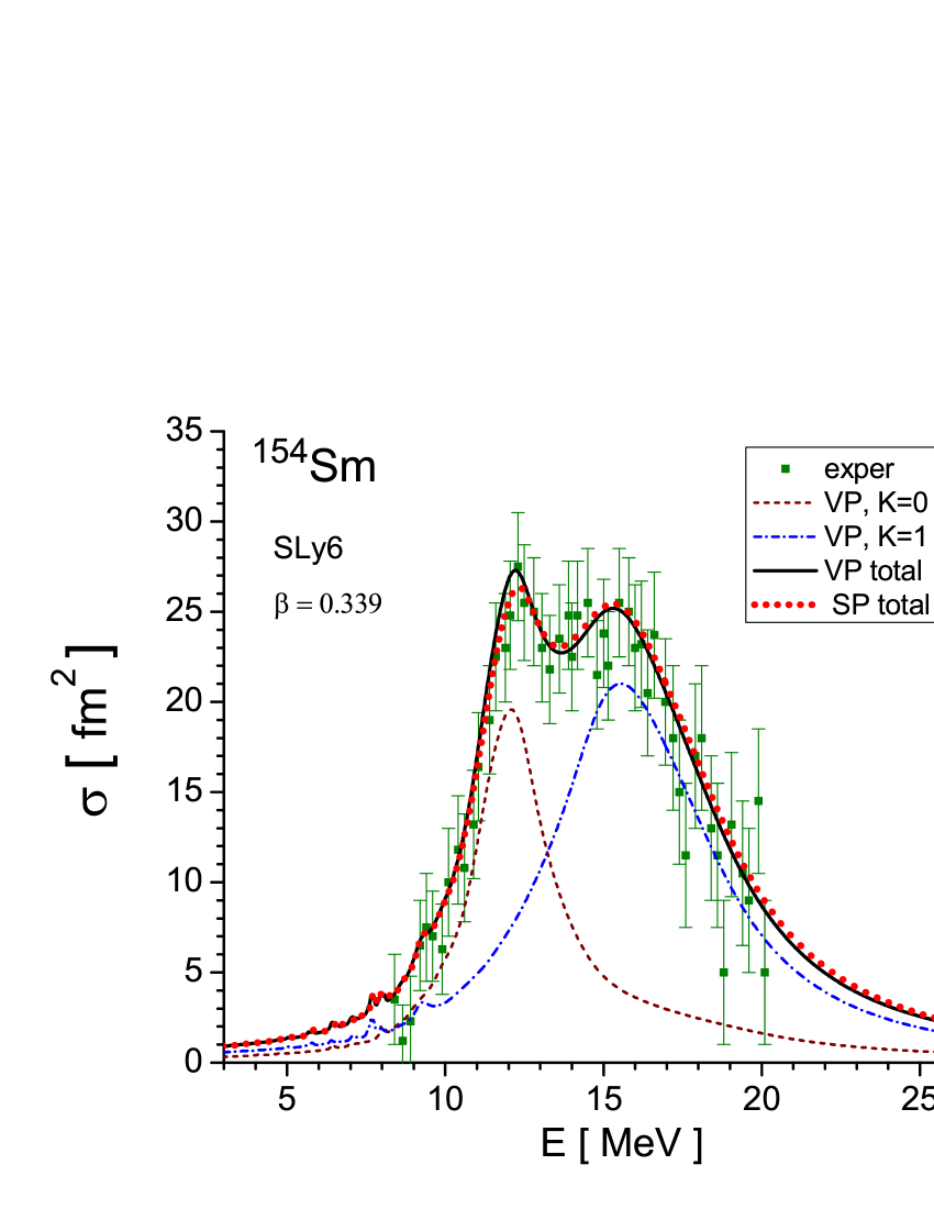
Figure 5: Calculated and experimental GDRexp photoabsorption cross-sections in ¹⁵⁴Sm. The total strengths are calculated with the pp-channel for VP and SP. For VP, $K=0$ and $K=1$ components are shown.

Fig. 5 compares the QRPA photoabsorption strength with the experimental data GDRexp . We see an excellent agreement between the theory and experiment. As said above, an appropriate modeling of the GDR shape is achieved by energy-dependent averaging described in Sec. 2.3. However, a correct description of peak position and, in a large extent, of fragmentation widths is achieved by QRPA with the parametrization SLy6. Altogether, the obtained agreement validates our approach for the further studies. Fig. 5 shows that VP and SP give almost identical results. The pp-channel does not have any effect (not shown since curves with and without the pp-channel almost coincide). The GDR exhibits deformation splitting into $K=0$ and $K=1$ branches. The sequence of branches is typical for GDR in prolate nuclei: $K=0$ branch lies below of $K=1$ one. Though $K=0$ branch involves about twice less strength than $K=1$ one, its peak height is a bit larger. This is explained by a stronger fragmentation of the $K=1$ branch, which broadens the distribution.

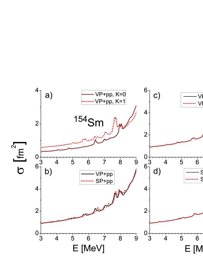
Figure 6: The calculated photoabsorption in the region of the pygmy resonance in ¹⁵⁴Sm. (a) K=0 and K=1 strengths with VP and pp-channel: b) total strengths (sums of $K=0$ and $K=1$ contributions) for VP and SP with pp-channel, c) total strengths for VP with and without pp-channel, d) the same as c) but for SP.

Fig. 6 shows the calculated photoabsorption in the PDR region. Following plots c)-d), the influence of the pp-channel is very weak for VP and SP (though for SP there are some small differences for the structures around 8 MeV). In the plot b), results from VP and SP deviate only in detail. Plot a) shows that $K=0$ strength exceeds $K=1$ strength at $E\geq$ 8 MeV but becomes smaller at $E\leq$ 8 MeV. A similar effect was found for Mo isotopes Mo . This is the result of the competition between GDR tails from $K=0$ and $K=1$ branches.

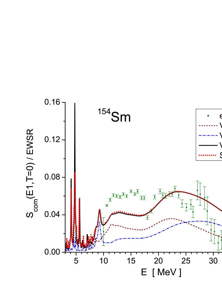
Figure 7: The compression isoscalar E1 strength (ISGDR) in ¹⁵⁴Sm, calculated with pp-channel for VP and SP cases. For VP, the $K=0$ and $K=1$ components are shown. The calculated strength is compared with the experimental data CDRexp . Calculated and experimental strengths are given as fractions of the corresponding EWSR(E1,T=0). See text for more detail.

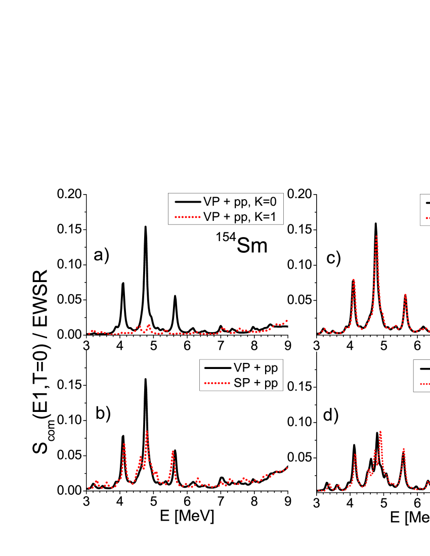
Figure 8: The calculated low-energy part of ISGDR in ¹⁵⁴Sm. (a) VP with pp channel: K=0 and K=1 components, b) VP and SP with pp-channel, c) VP with and without pp-channel, d) SP with and without pp-channel.

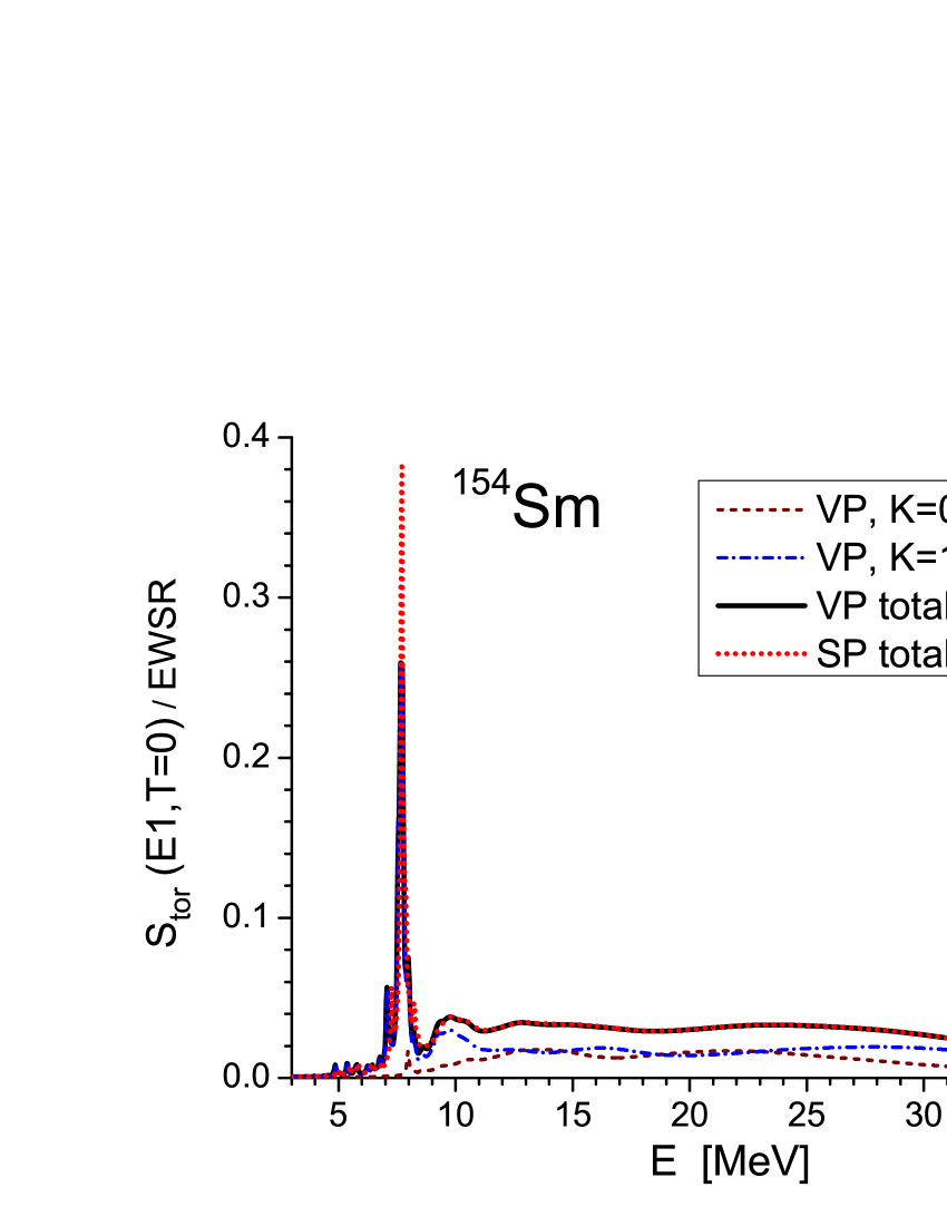
Figure 9: The isoscalar toroidal E1 strength function in ¹⁵⁴Sm, calculated for volume (VP) and surface (SP) pairing. In both cases, the pp-channel is included. For VP, the $K=0$ and $K=1$ components are shown.

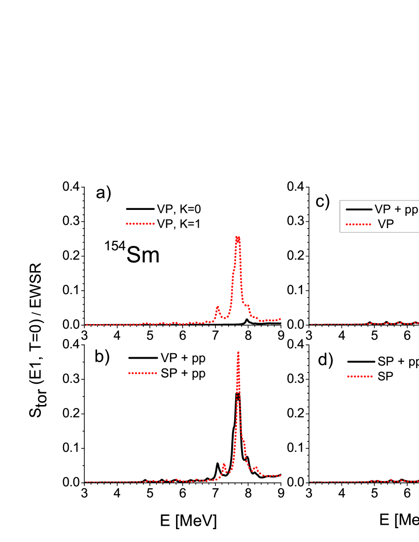
Figure 10: The calculated low-energy isoscalar toroidal E1 strength in ¹⁵⁴Sm. (a) VP with pp channel: $K=0$ and $K=1$ components, b) VP and SP with pp-channel, c) VP with and without pp-channel, d) SP with and without pp-channel.

Fig. 7 shows the QRPA isoscalar dipole strength (ISGDR) as a fraction of the computed energy-weighted sum rule EWSR(E1,T=0)=$\int dES_{\rm com}(E1,T=0;E)$ (a similar presentation but in terms of experimental EWSR is used for experimental data CDRexp ). We see that, in agreement with experiment, the computed ISGDR includes two broad bumps at 10-17 and 17-40 MeV. Similar bumps were also observed in other (spherical) nuclei CDRexp ; Young90Zr ; Uch04 . They are often treated as TDR and CDR respectively, see e.g. CDRexp . However, our previous studies Re13 ; Kv13Sm ; Kv14Yb ; Ne17 ; NeDre14 for different nuclei and present analysis for ¹⁵⁴Sm suggest that both broad bumps in ISGDR belong to CDR. Comparison of Figs. 7 and 9 shows that even spikes at 4–6 MeV can hardly be considered as being toroidal because they are almost absent in the toroidal distributions shown in Figs. 9 and 10.

Fig. 7 demonstrates that strengths obtained with VP and SP are almost identical. The effect of the pp-channel for the strength at $E>$ 10 MeV is negligible (not shown). Concerning the deformation effects, $K=0$ and $K=1$ branches show the familiar sequence (like in GDR) at E=10-40 MeV, namely that the $K=0$ branch lies below the $K=1$ branch.

The ISGDR strength at lower energies is shown in Fig. 8. Plot a) demonstrates that $K=1$ strength dominates at E=8–10 MeV but becomes weaker at 3–8 MeV. So, at 3–8 MeV, the ratio of $K=0$ and $K=1$ strengths is opposite to that in PRD. Plots b)-d) of Fig. 8) also show very close results for VP as compared to SP and an almost negligible effect of the pp-channel.

Figure 11: The isoscalar QRPA current transition densities in x-z plane for dipole excitations at 6–9 MeV in ¹⁵⁴Sm: a) $K=0$, b) $K=1$. The currents are obtained for VP. Magnitude of the current is determined by arrow length (in arbitrary units). The nuclear surface is indicated by the solid line.

Fig. 9 shows the toroidal isoscalar strength function obtained with the transition operator (21) as a fraction of the integral toroidal strength (EWSR). We see that the strength has a broad plateau at 10–40 MeV. Most probably such a broad distribution is caused by the coupling between TDR and CDR Kv11 . In this plateau, the $K=1$ strength dominates at $E>$ 25 MeV. Below, at 12–25 MeV, the $K=0$ and $K=1$ strengths are about the same. Even lower, at $E<$ 12 MeV, the $K=1$ strength becomes strongly dominant. In particular a strong toroidal peak at 7–8 MeV is almost fully built from $K=1$ strength. Note that SP makes this peak essentially higher than VP. Perhaps this happens because the toroidal $K$=1 motion is strongest just at the nuclear surface, see Fig. 11 below. So the description of the TDR peak depends on the sort of the pairing. This is the only place where we could observes a significant difference between VP and SP.

The TDR strength is presented in more detail in Fig. 10. Plot b) demonstrates a significant difference between VP and SP results for the highest TDR peak. Plots c) and d) show a negligible contribution of the pp-channel. Further, plot a) confirms that the TDR strength is almost fully provided by $K$=1 contribution. This peculiarity of the TDR corresponds to the PDR picture (where $K$=1 strength also dominates at $E<$ 8 MeV) but is opposite to low-energy part of the CDR with dominant $K$=0 strength. It is interesting that the PDR peaks roughly correspond to the PDR structures at 7–8 MeV but have no counterpart in the low-energy CDR located at 4-6 MeV. This is one more indication for the intimate relation between TDR and PDR, discussed in Re13 . Note that the peaked TDR strength appears even in the unperturbed (without residual interaction) strength function NeDre14 . The isoscalar residual interaction only downshifts the structure by $\sim$ 2 MeV.

To illustrate the mainly toroidal nature of dipole states at 6–9 MeV, we show in Fig. 11 their isoscalar average current transition densities (CTD) for the branches $K=0$ and $K=1$. The method of calculation of the average CTD in QRPA is described in detail in Re13 . Remind that CTD depend only on the structure of QRPA states and are not affected by the probing external field. In Fig. 11, we see for both $K=0$ and $K=1$ basically toroidal flow. The toroidal axes are directed along z-axis for $K=0$ and x-axis for $K=1$. It is interesting that the toroidal flow resembles a vortex-antivortex configuration. Fig. 11 shows that for $K=1$ the flow is much stronger, especially at the nuclear surface. This supports the previous finding that the TDR is mainly realized in the $K=1$ branch. Perhaps, the nuclear geometry in the $K=1$ case is more suitable for hosting the toroidal flow and thus makes the flow more energetically favorable. Our analysis shows that the strong $K=1$ flow at the nuclear surface is mainly provided by neutrons. The strong motion of the neutron surface against the remaining core corresponds to a typical PDR picture. So Fig. 11 confirms our previous suggestion Re13 that PDR is mainly a local boundary manifestation of the toroidal nuclear flow.

Figure 12: The same as in Fig. 11 but for dipole excitations at 3–6 MeV.

Finally, Fig. 12 shows the currents for the dipole excitations at 3–6 MeV (exhibited at Fig. 8a). The flow considerably deviates from the toroidal picture.

Altogether, Figs. 5–12 show that in the dipole resonances (GDR, PDR, TDR, CDR): i) the pp-channel is negligible; ii) the difference between VP and SP results is small (except for the strongest TDR peak at 7–8 MeV); iii) at $E>$ 10 MeV, the familiar sequence of $K=$0 and $K=$1 branches is observed; iv) at $E<$ 10 MeV, the ratio between the branches depends on the resonance ($K=1$ strength dominates in TDR and PDR but becomes minor in CDR); v) The $K=1$ strength forms an impressively narrow low-energy peak in the TDR (the latter feature may serve as a fingerprint of the TDR in future experiments); vi) current transition densities (CTD) confirm the mainly toroidal nature of dipole excitations at 6–9 MeV.

Figs. 5–12 allow to do some additional comments concerning origin of PDR and ISGDR, deformation splitting of these resonances, and perspectives of experimental observation of TDR.

1) The TDR operator (21) has the radial dependence $\sim r^{2}$ and so surface reactions should be sensitive probes of this resonance. In particular, the ($\alpha,\alpha^{\prime}\gamma$) reaction in deformed nuclei looks suitable to excite the isoscalar TDR and determine, using Alaga rules Ala55 , a dominant K=1 low-energy TDR peak. The ratio of intensities of $E1K$-transitions from a given dipole QRPA $K$-state to the members $I^{\pi}K=0^{+}0$ and $2^{+}0$ of the ground-state rotational band is determined through Clebsh-Gordan coefficients as

$$A_{K}=|\frac{\langle 1K1-K|00\rangle}{\langle 1K1-K|20\rangle}|^{2}.$$ (23)

This yields $A_{0}$=0.5 and $A_{1}$=2. Thus $K=0$ and $K=1$ branches can be distinguished. Although these dipole transitions are isoscalar, they should be strong enough to be detectable since the peaked TDR is a collective mode Kv14Yb ; Ne17 ; NeDre14 . Note that in ¹⁵⁴Sm the TDR peak lies below the neutron and proton threshold energies, which should favor its $\gamma$-decay.

2) The relevance of the ($\alpha,\alpha^{\prime}\gamma$) reaction to observe the TDR is not so evident. Note that, despite the TDR/CDR relation, the irrotational ISGDR strength in Figs. 7-8 does not match the vortical toroidal strength exhibited in Figs. 9-10. There is a general question if the ($\alpha,\alpha^{\prime}$) reaction is, in principle, able to probe vortical modes. We need here further analysis. From the theoretical side, DWBA calculations for ($\alpha,\alpha^{\prime}$) angular distributions should be performed, using QRPA input formfactors for the TDR low-energy $K=1$ peak.

3) Following our results, the ISGDR observed at 10-33 MeV in $(\alpha,\alpha^{\prime})$ scattering to small angles CDRexp is perhaps a fully irrotational mode dominated by compression-like dipole excitations. In other words, the observed ISGDR does not include the TDR at all. Indeed both observed broad bumps at 10-17 MeV and 17-33 MeV are located higher than the TDR peak predicted at 7-8 MeV. Moreover, in this experiment, only excitations at $E>$ 10MeV are measured, i.e. the actual TDR energy region is fully omitted. In the same experiment for other nuclei (¹¹⁶Sn, ¹⁴⁴Sm and ²⁰⁸Pb) the TDR low-energy region was also missed CDRexp . At the same time, some low-energy peaks (which can be attributed to the TDR) were measured in ⁹⁰Zr, ¹¹⁶Sn, ¹⁴⁴Sm and ²⁰⁸Pb in an alternative $(\alpha,\alpha^{\prime})$ experiment Uch04 where the interval $E>$ 8 MeV was inspected. These peaks can match a part of the TDR. However we still need measurements for the lower energy interval which fully embraces the predicted TDR.

4) As discussed in Re13 , the PDR is probably a complicated mixture of various dipole excitations (toroidal, compression, GDR tail) with a dominant contribution of the toroidal fraction. Following Figs. 6, 8, 10, the dipole response crucially depends on the probe. The PDR structure in deformed nuclei (K-branches) also should depend on the reaction applied. For example, following Figs. 8 and 10, $K$-branches of the PDR can arise separately as responses to different probes: $K$=0 in the CDR/ISGDR response and $K=1$ in the toroidal response. If so, then investigation of CDR/ISGDR and TDR could be useful to understand the deformation splitting of the PDR.

IV Conclusions

Effects of nuclear deformation and monopole pairing in nuclear excitations with $K^{\pi}\neq 0^{+}$ were investigated within the self-consistent Quasiparticle Random Phase Approximation (QRPA) method Re16 using the Skyrme parametrization SLy6 Cha97 . Mean field and pairing were treated within the HF+BCS scheme. As representative examples the axially deformed nuclei ^152,154,156Sm were considered. One of the main aims was to investigate the role of the particle-particle (pp) channel in the residual QRPA interaction. This channel is known to be important for $K^{\pi}=0^{+}$ states SSS ; Ri80 but its role in $K^{\pi}\neq 0^{+}$ excitations was yet unclear. We scrutinized this problem for the lowest $\gamma$-vibrational $K^{\pi}=2^{+}$ states and for dipole low- and high-energy excitations: isovector giant dipole resonance (GDR), isovector pygmy dipole resonance (PDR), toroidal dipole resonance (TDR), and compression dipole resonance (CDR). We also compared QRPA results for these excitations with volume and surface pairing. Last but not least, we analyzed deformation effects in the dipole resonances, especially in the low-energy interval where PDR is located. The following results have been obtained:
1) The effect of the pp-channel in $K^{\pi}\neq 0^{+}$ excitations is negligible. This can be explained by the absence of the proton-neutron part in the pairing forces (though the proton-neutron interaction dominates in the ph-channel). As a result, the pp-channel turns out to be much weaker than its ph-counterpart and finally can be safely neglected in description of $K^{\pi}\neq 0^{+}$ modes. This result is important from the practical side because omitting the pp-channel considerably simplifies QRPA calculations, which is especially beneficial for deformed nuclei where QRPA calculations are time-consuming. Since the effect of the pp-channel is fairly small, its omission does not spoil the consistency of QRPA. In our study, this result was obtained for low-energy $K^{\pi}=2^{+}$ states and dipole resonances. However it is likely to be valid for any nuclear excitation with $K^{\pi}\neq 0^{+}$ (dipole, quadrupole, octupole).
2) Our calculations have shown that, as a rule, the difference between the QRPA results obtained with from volume pairing (VP) and from surface pairing (SP) is small. A noticeable difference was found only for the collective low-energy peak of the TDR.
3) We analyzed deformation effects arising due to competition between $K=0$ and $K=1$ branches in the dipole excitations, comparing the behavior of the branches in various dipole resonances (GDR, PDR, TDR, CDR). It was shown that, in all the resonances, the familiar sequence of $K=0$ and $K=1$ branches takes place for excitation energy $E>$ 10 MeV, namely the $K=0$ structure lies lower than the $K=1$ one as it should be in prolate nuclei. However, at lower excitation energies $E<$ 10 MeV, the behavior of the branches depends on the resonance type. In particular, in the PDR and TDR, the $K=1$ strength becomes dominant. For TDR, this effect manifests itself in the appearance of very strong peak at $\sim$ 7–8 MeV, which is almost completely built from $K=1$ strength. This remarkable feature can be used as a fingerprint of the TDR in future experiments. The ($\alpha,\alpha^{\prime}\gamma$) reaction in deformed nuclei looks most promising. The peaked $K=1$ strength can be identified inspecting intensities of the $\gamma$-decay in terms of Alaga rules.
4) Following our results, the ISGDR observed in $(\alpha,\alpha^{\prime})$ scattering to forward angles CDRexp is basically irrotational and perhaps does not include at all the low-energy vortical TDR. To search the TDR, the lower excitation energies should be experimentally inspected.
5)The nuclear flow in the PDR energy region is basically toroidal. The deformation structure of PDR can be related to $K$ branches in TDR and CDR.

The work was partly supported by Votruba-Blokhincev (Czech Republic-BLTP JINR) and Heisenberg-Landau (Germany - BLTP JINR) grants. The support of the Czech Scinece Foundation Grant Agency (project P203-13-07117S) is appreciated. A.R. is grateful for support from Slovak Research and Development Agency under Contract No. APVV-15-0225.

Appendix A Skyrme functional

The Skyrme energy functional (1) has the kinetic-energy, Skyrme, Coulomb and pairing parts Be03 ; Rei92d with ($q=n,p$)

$$\mathcal{E}_{\rm kin}=\int\mathrm{d}\vec{r}\sum_{q}\frac{\hbar^{2}}{2m_{q}}\tau_{q}(\vec{r}),$$ (A.1)

$$\mathcal{E}_{\rm Sk}=\int\mathrm{d}\vec{r}\bigg{\{}\frac{b_{0}}{2}\rho^{2}-\frac{b_{0}^{\prime}}{2}\sum_{q}\rho_{q}^{2}+\frac{b_{2}}{2}(\vec{\nabla}\rho)^{2}$$ (A.2)

$$-\frac{b_{2}^{\prime}}{2}\sum_{q}(\vec{\nabla}\rho_{q})^{2}+b_{1}(\rho\tau\!-\!\vec{j}^{\,2})-b_{1}^{\prime}\sum_{q}(\rho_{q}\tau_{q}\!-\!\vec{j}_{q}^{\,2})$$

$$+\tilde{b}_{1}\Big{(}\vec{s}\cdot\vec{T}-{\bf J}^{2}\Big{)}+\tilde{b}_{1}^{\prime}\sum_{q}\Big{(}\vec{s}_{q}\cdot\vec{T}_{q}-{\bf J}_{q}^{2}\Big{)}$$

$$+\frac{b_{3}}{3}\rho^{\alpha+2}-\frac{b_{3}^{\prime}}{3}\rho^{\alpha}\sum_{q}\rho_{q}^{2}-b_{4}\big{[}\rho\vec{\nabla}\cdot\vec{J}+\vec{s}\cdot(\vec{\nabla}\times\vec{j})\big{]}$$

$$-b_{4}^{\prime}\sum_{q}\big{[}\rho_{q}\vec{\nabla}\cdot\vec{J}_{q}+\vec{s}_{q}\cdot(\vec{\nabla}\times\vec{j}_{q})\big{]}$$

$$+\frac{\tilde{b}_{0}}{2}\vec{s}^{2}-\frac{\tilde{b}_{0}^{\prime}}{2}\sum_{q}\vec{s}_{q}^{\,2}+\frac{\tilde{b}_{2}}{2}\sum_{ij}(\nabla_{i}s_{j})^{2}$$

$$-\frac{\tilde{b}_{2}^{\prime}}{2}\sum_{q}\sum_{ij}(\nabla_{i}s_{j})_{q}^{2}+\frac{\tilde{b}_{3}}{3}\rho^{\alpha}\vec{s}^{\,2}-\frac{\tilde{b}_{3}^{\prime}}{3}\rho^{\alpha}\sum_{q}\vec{s}_{q}^{\,2}\bigg{\}}\>,$$

$$\mathcal{E}_{\rm Coul}=\frac{1}{2}e^{2}\int\mathrm{d}\vec{r}\int\mathrm{d}\vec{r}^{\prime}\frac{\rho_{p}(\vec{r})\rho_{p}(\vec{r}^{\prime})}{|\vec{r}-\vec{r}^{\prime}|}$$ (A.3)

$$\qquad\qquad\qquad-\frac{3}{4}\Big{(}\frac{3}{\pi}\Big{)}^{\frac{1}{3}}e^{2}\int\mathrm{d}\vec{r}\rho_{p}(\vec{r})^{\frac{4}{3}}.$$

The pairing part is given in Eq. (3) of Section 2.2. The functional depends on time-even ($\rho$, $\tau$, ${\bf J}$, $\tilde{\rho}$) and time-odd ($\vec{j}$, $\vec{s}$, $\vec{T}$) local densities and currents. The total densities are sums of the proton and neutron parts, e.g. $\rho=\rho_{n}+\rho_{p}$. In HF+BCS approach, the densities of our main interest, nucleon $\rho$ and pairing $\tilde{\rho}$, have the form (6) and (7). The relation of the Skyrme parameters $b_{i}$ with the standard ones $t_{i},\>x_{i}$ can be found in Re16 ; Be03 ; Rei92d

Appendix B HF+BCS equations

The zero-range monopole pairing is defined by Eqs. (3)-(5). It results in the BCS equations:

$$[u_{i}^{q}]^{2}=\frac{1}{2}\>\left\{1+\frac{e_{i}^{q}-\lambda_{q}}{\sqrt{\left[e_{i}^{q}-\lambda_{q}\right]^{2}+[\Delta_{i}^{q}]^{2}}}\right\},$$ (B.1)

$$[v^{q}_{i}]^{2}=\frac{1}{2}\>\left\{1-\frac{e_{i}^{q}-\lambda_{q}}{\sqrt{\left[e_{i}^{q}-\lambda_{q}\right]^{2}+[\Delta_{i}^{q}]^{2}}}\right\},$$ (B.2)

$$\Delta_{i}^{q}=-\sum_{j\in q}^{K>0}f_{j}^{q}V^{(\rm{pair},q)}_{i\bar{i}j\bar{j}}\>v_{j}^{q}u_{j}^{q},$$ (B.3)

$$N_{q}=\sum_{i\in q}^{K>0}f_{i}^{q}\left\{1-\frac{e_{i}^{q}-\lambda_{q}}{\sqrt{\left[e_{i}^{q}-\lambda_{q}\right]^{2}+[\Delta_{i}^{q}]^{2}}}\right\},$$ (B.4)

where $e_{i}^{q}$ is the s-p energy, $u_{i}^{q},v_{i}^{q}$ are Bogoliubov coefficients, $\Delta_{i}^{q}$ is the pairing gap, $\lambda_{q}$ is the chemical potential, $f_{i}^{q}$ is the cut-off function (2), $N_{p}=Z$ and $N_{n}=N$ are proton and neutron numbers, and $V_{i\bar{i}j\bar{j}}^{(\rm{pair,q})}=\langle i\bar{i}|V^{q}_{\rm pair}(\vec{r},\vec{r}^{\prime})|j\bar{j}\rangle$ is the pairing matrix element.

The total HF+BCS Hamiltonians consists from the local pairing and HF parts:

$${\hat{h}}^{q}_{\rm HF+BCS}(\rho,{\tilde{\rho}})={\hat{h}}^{q}_{\rm pair}(\rho,{\tilde{\rho}})+{\hat{h}}^{q}_{\rm HF}(\rho,\tau,{\bf J},\tilde{\rho}).$$ (B.5)

The pairing part

$${\hat{h}}^{q}_{\rm pair}(\rho,{\tilde{\rho}})(\vec{r})=\frac{\delta\mathcal{E}_{\rm pair}}{\delta{\tilde{\rho}_{q}}(\vec{r})}=\frac{1}{2}{\tilde{\rho}_{q}}(\vec{r})G_{q}(\vec{r})$$ (B.6)

depends on the pairing density $\tilde{\rho}$ and, in SP case, on total nucleon density $\rho$ (through the factor $G_{q}(\vec{r})$).

The mean-field part

$${\hat{h}}^{q}_{\rm HF}(\rho,\tau,{\bf J},\tilde{\rho})(\vec{r})=\frac{\delta\mathcal{E}}{\delta\rho_{q}(\vec{r})}+\frac{\delta\mathcal{E}}{\delta\tau_{q}(\vec{r})}+\frac{\delta\mathcal{E}}{\delta\mathbf{J}_{q}(\vec{r})}$$ (B.7)

is determined by the time-even densities involved to the Skyrme functional (A.2). For SP, the Hamiltonian (B.7) gains dependence on the pairing density $\tilde{\rho}$.

BCS equations (B.1)-(B.4) are coupled to the density-dependent HF equations

$${\hat{h}}^{q}_{\rm HF}(\rho,\tau,{\bf J},\tilde{\rho})(\vec{r})\psi^{q}_{i}(\vec{r})=e_{i}^{q}\psi^{q}_{i}(\vec{r})$$ (B.8)

via the pairing $u_{i}^{q},v_{i}^{q}$-factors in the densities, see e.g. Eq. (6) for $\rho_{q}(\vec{r})$. In turn, the BCS equations are affected by the HF mean field through single-particle energies $e_{i}^{q}$ and wave functions $\psi_{i}^{q}$. In our HF+BCS scheme, BCS equations (B.1)–(B.4) are solved at each HF iteration Skyax .

Appendix C QRPA with pp-channel

The QRPA equations read Ri80

$$\left(\begin{array}[]{cc}A&B\\ B^{*}&A^{*}\end{array}\right)\left(\begin{array}[]{c}X^{(\nu)}\\ Y^{(\nu)}\end{array}\right)=\hbar E_{\nu}\>\left(\begin{array}[]{cc}1&0\\ 0&-1\end{array}\right)\left(\begin{array}[]{c}X^{(\nu)}\\ Y^{(\nu)}\end{array}\right)$$ (C.1)

where $X^{(\nu)}_{ij}$ and $Y^{(\nu)}_{ij}$ are forward and backward amplitudes of QRPA phonon creation operators $Q^{+}_{\nu}$

$$Q^{+}_{\nu}=\frac{1}{2}\sum_{ij}\big{(}X^{(\nu)}_{ij}\>\alpha^{+}_{i}\alpha^{+}_{j}-Y^{(\nu)}_{ij}\>\alpha_{j}\>\alpha_{i}\big{)},$$ (C.2)

$E_{\nu}$ is the phonon energy, $\alpha^{+}_{i}(\alpha_{j})$ is the quasiparticle creation (annihilation) operator. The RPA matrices $A$ and $B$ have the form

$$A_{\omega\omega^{\prime}} = \epsilon_{\omega}\delta_{\omega,\>\omega^{{}^{\prime}}}$$

$$+ \sum_{d\>d^{\>{}^{\prime}}}\int\!\!\mathrm{d}\vec{r}\!\int\!\!\mathrm{d}\vec{r}^{\prime}\frac{\delta^{2}\mathcal{E}}{\delta\mathcal{J}^{d}(\vec{r})\>\delta\mathcal{J}^{d^{\prime}}(\vec{r^{{}^{\prime}}})}\>\delta\mathcal{J}^{d}_{\omega}(\vec{r})\>\delta\mathcal{J}^{d^{\prime}}_{\omega^{\prime}}(\vec{r}^{\prime})$$

$$B_{\omega\omega^{{}^{\prime}}} = -\>\sum_{d\>d^{\>{}^{\prime}}}\int\!\!\mathrm{d}\vec{r}\!\int\!\!\mathrm{d}\vec{r}^{\prime}\frac{\delta^{2}\mathcal{E}}{\delta\mathcal{J}^{d}(\vec{r})\>\delta\mathcal{J}^{d^{\prime}}(\vec{r^{{}^{\prime}}})}\>\delta\mathcal{J}^{d}_{\omega}(\vec{r})\>\delta\mathcal{J}^{d^{\prime}}_{\omega^{\prime}}(\vec{r}^{\prime})$$

where $\omega=ij,\>\bar{i}\bar{j},\>i\bar{j}\in q$ and $\omega^{\prime}=i^{\prime}j^{\prime},\>\bar{i}^{\prime}\bar{j}^{\prime},\>i^{\prime}\bar{j}^{\prime}\in q^{\prime}$ ($i>j$); $\delta_{ij,\>i^{{}^{\prime}}j^{{}^{\prime}}}\equiv\delta_{ii^{{}^{\prime}}}\delta_{jj^{{}^{\prime}}}-\delta_{ij^{{}^{\prime}}}\delta_{j\>i^{{}^{\prime}}}$, $\delta_{i\>\bar{j},\>i^{{}^{\prime}}\bar{j^{{}^{\prime}}}}\equiv\delta_{ii^{{}^{\prime}}}\delta_{jj^{{}^{\prime}}}$, $\delta_{ij,\>i^{{}^{\prime}}\bar{j^{{}^{\prime}}}}=0$. Further, $\epsilon_{\omega}\equiv\epsilon_{i}+\epsilon_{j}$ is 2qp energy; $\delta\mathcal{J}^{d}_{\omega}(\vec{r})=\langle\omega|\hat{\mathcal{J}}^{d}|0\rangle$ is the transition density for the transition between 2qp state $|\omega\rangle$ and BCS vacuum $|0\rangle$, $\hat{\mathcal{J}}^{d}$ is the density operator in 2qp representation (in terms of $\alpha^{+}_{i}\alpha^{+}_{j},\>\alpha_{i}\alpha_{j}$); the set $\mathcal{J}^{d}$ includes the densities and currents $d\in\>\rho,\>\tau,\>{\bf J},\>\vec{j},\>\vec{s},\>\vec{T},\tilde{\rho}$. For more details see Re16 .

The pairing functional $\mathcal{E}_{\rm pair}$ (3) leads to additional terms in the residual interaction, which constitute the pp-channel:

$$\frac{\delta^{2}\mathcal{E}}{\delta\rho(\vec{r})\>\delta\rho(\vec{r}^{{}^{\prime}})},\>\frac{\delta^{2}\mathcal{E}}{\delta\rho(\vec{r})\>\delta\tilde{\rho}(\vec{r}^{{}^{\prime}})},\>\frac{\delta^{2}\mathcal{E}}{\delta\tilde{\rho}(\vec{r})\>\delta\rho(\vec{r}^{{}^{\prime}})},\>\frac{\delta^{2}\mathcal{E}}{\delta\tilde{\rho}(\vec{r})\>\delta\tilde{\rho}(\vec{r}^{{}^{\prime}})}.$$

In SP, all the terms take place while in VP only the last term remains. In the QRPA matrices $A$ and $B$, the pp-channel is presented by the terms:

$$A^{\rm pair}_{qq^{\prime}}(ij,i^{\prime}j^{\prime})=-\frac{\eta\>\gamma\>(\gamma-1)}{4\>\rho^{\gamma}_{0}}$$ (C.4)

$$\cdot \sum_{q=n,p}V_{q}\>\int\mathrm{d}\vec{r}\>\tilde{\rho}^{2}_{q}(\vec{r})\>\>\rho^{\gamma-2}(\vec{r})\>\delta\rho_{ij}(\vec{r})\>\delta\rho_{i^{\prime}j^{\prime}}(\vec{r}),$$

$$B^{\rm pair}_{qq^{\prime}}(ij,i^{\prime}j^{\prime})=-\>A^{\rm pair}_{qq^{\prime}}(ij,i^{\prime}j^{\prime}),$$

$$\>A^{\rm pair}_{qq^{\prime}}(i\bar{j},i^{\prime}\bar{j}^{\prime})=-\frac{\eta\>\gamma\>(\gamma-1)}{4\>\rho^{\gamma}_{0}}$$ (C.6)

$$\cdot \sum_{q=n,p}V_{q}\>\int\mathrm{d}\vec{r}\>\tilde{\rho}^{2}_{t}(\vec{r})\>\>\rho^{\gamma-2}(\vec{r})\delta\rho_{ij}(\vec{r})\>\delta\rho_{i^{\prime}j^{\prime}}(\vec{r})$$

$$+\frac{1}{2}\>\delta_{qq^{\prime}}V_{q}\>\int\mathrm{d}\vec{r}\Big{[}1-\eta\>\Big{(}\frac{\rho(\vec{r})}{\rho_{0}}\Big{)}^{\gamma}\Big{]}\delta\tilde{\rho}_{ij}(\vec{r})\>\delta\tilde{\rho}_{i^{\prime}j^{\prime}}(\vec{r})$$

$$-\frac{\eta\>\gamma}{2\rho_{0}^{\gamma}}\>V_{q}\>\int\mathrm{d}\vec{r}\>\tilde{\rho}_{q}(\vec{r})\>\rho^{\gamma-1}(\vec{r})\delta\tilde{\rho}_{ij}(\vec{r})\>\delta\rho_{i^{\prime}j^{\prime}}(\vec{r})$$

$$-\frac{\eta\>\gamma}{2\rho_{0}^{\gamma}}\>V_{q^{{}^{\prime}}}\>\int\mathrm{d}\vec{r}\>\tilde{\rho}_{q^{{}^{\prime}}}(\vec{r})\>\rho^{\gamma-1}(\vec{r})\delta\rho_{ij}(\vec{r})\>\delta\tilde{\rho}_{i^{\prime}j^{\prime}}(\vec{r})$$

$$B^{\rm pair}_{qq^{\prime}}(i\bar{j},i^{\prime}\bar{j}^{\prime})=-\>A^{\rm pair}_{qq^{\prime}}(i\bar{j},i^{\prime}\bar{j}^{\prime}),$$

The contributions (C.4)-(C.4) and the first term in (C.6) are zero for both VP ($\eta$=0) and SP (if $\gamma$=1). The last two cross terms in (C.6) exist only for the density-dependent SP (when $\eta\neq$ 0). Only the second term in (C.6), including merely pairing transitions densities $\delta\tilde{\rho}$, exists for both VP and SP. Expressions (C.4)-(C.6) correspond to the formalism derived in Te05 for spherical nuclei.

Expressions (C.4)-(C.6) include contributions to pp-channel from both diagonal ($i=j$) and non-diagonal ($i\neq j$) 2qp configurations. Note that, in the quasiparticle-phonon model (QPM) with the constant pairing SSS , only diagonal contributions are taken into account, thus the pp-channel exists only for $K^{\pi}=0^{+}$ states. In our study for states with $K^{\pi}\neq 0^{+}$, the selection rules allow only non-diagonal configurations.

References

- (1) V.G. Soloviev, A.V. Sushkov, N.Yu. Shirikova, Phys. Part. Nucl. 25, 377 (1994); ibid 27, 1643 (1996).
- (2) P. Ring, P. Schuck, The Nuclear Many-Body Problem (Springer-Verlag, Berlin, 1980).
- (3) J. Dobaczewski, H. Flocard, J. Treiner, Nucl. Phys. A 422, 103 (1984).
- (4) J. Dobaczewski, W. Nazarewicz, T.R. Werner, J.F. Berger, C.R. Chinn, J. Dechargé, Phys. Rev. C 53, 2809 (1996).
- (5) P.-G. Reinhard, M. Bender, K. Rutz, J.A. Maruhn, Z. Phys. A 358, 277 (1997).
- (6) M. Bender, K. Rutz, P.-G. Reinhard, J.A. Maruhn, Eur. Phys. J. A 8, 59 (2000).
- (7) N. Tajima, Phys. Rev. C 69 034305 (2004).
- (8) J. Terasaki, J. Engel, M. Bender, J. Dobaczewski, W. Nazarewicz, M. Stoitsov, Phys. Rev. C 71, 034310 (2005).
- (9) J. Li, G. Colò, J. Meng, Phys. Rev. C 78, 064304 (2008).
- (10) N. Lo Iudice, A. V. Sushkov, and N. Yu. Shirikova, Phys. Rev. C 72, 034303 (2005).
- (11) A.P. Severyukhin, V.V. Voronov, Nguyen Van Giai, Phys. Rev. C 77, 024322 (2008).
- (12) J. Terasaki, J. Engel, Phys. Rev. C 82, 034326 (2010).
- (13) J. Terasaki, J. Engel, Phys. Rev. C 84, 014332 (2011).
- (14) A. Repko, arXiv:1603.04383v2 [nucl-th].
- (15) E. Chabanat, P. Bonche, P. Haensel, J. Meyer, R. Schaeffer, Nucl. Phys. A 635, 231 (1998).
- (16) V.O. Nesterenko, V.G. Kartavenko, W. Kleinig, J. Kvasil, A. Repko, R.V. Jolos, P.-G. Reinhard, Phys. Rev. C 93, 034301 (2016).
- (17) N. Paar, D. Vretenar, E. Khan, G. Colò, Rep. Prog. Phys. 70, 691 (2007).
- (18) J. Kvasil, V.O. Nesterenko, W. Kleinig, P.-G. Reinhard, P. Vesely, Phys. Rev. C 84, 034303 (2011).
- (19) A. Repko, P.-G. Reinhard, V.O. Nesterenko, J. Kvasil, Phys. Rev. C 87, 024305 (2013).
- (20) M.N. Harakeh, A. van der Woude, Giant Resonances ( Oxford, Clarendon, 2001).
- (21) J. Kvasil, V.O. Nesterenko, W. Kleinig, D. Bozik, P.-G. Reinhard, N. Lo Iudice, Eur. Phys. J. A 49, 119 (2013).
- (22) J. Kvasil, V.O. Nesterenko, W. Kleinig, P.-G. Reinhard, Phys. Scr. 89, 054023 (2014).
- (23) V.O. Nesterenko, J. Kvasil, A. Repko, W. Kleinig, P.-G. Reinhard, Phys. Atom. Nucl. 79, 842 (2016).
- (24) T.H.R. Skyrme, Phil. Mag. 1, 1043 (1956).
- (25) D. Vautherin, D.M. Brink, Phys. Rev. C 5, 626 (1972).
- (26) M. Bender, P.-H. Heenen, P.-G. Reinhard, Rev. Mod. Phys. 75, 121 (2003).
- (27) W. Kleinig, V.O. Nesterenko, J. Kvasil, P.-G. Reinhard, P. Vesely, Phys. Rev. C 78, 044313 (2008).
- (28) Evaluated Nuclear Structure Data File, http://www.nndc.bnl.gov/chart/.
- (29) P.–G. Reinhard, Ann. Phys. (Leipzig) 504, 632 (1992).
- (30) P. Klüpfel, P.–G. Reinhard, T. J. Bürvenich, and J. A. Maruhn, Phys. Rev. C 79, 034310 (2009).
- (31) V.O. Nesterenko, W. Kleinig, J. Kvasil, P. Vesely, P.-G. Reinhard, D.S. Dolci, Phys. Rev. C 74, 064306 (2006).
- (32) P. Fleischer, P. Klupfel, P.-G. Reinhard, and J. A. Maruhn, Phys. Rev. C 70, 054321 (2004).
- (33) G.M. Gurevich, L.E. Lazareva, V.M. Mazur, S.Yu. Merkulov, G.V. Solodukhov, V.A. Tyutin, Nucl. Phys. A 351, 257 (1981).
- (34) J. Kvasil, P. Vesely, V.O. Nesterenko W. Kleinig, P.-G. Reinhard, S. Frauendorf, Int. J. Mod. Phys. E 18, 975 (2009).
- (35) D.H. Youngblood, Y.-W. Lui, H.L. Clark, B. John, Y. Tokimoto, X. Chen, Phys. Rev. C 69, 034315 (2004).
- (36) D. H. Youngblood, Y.-W. Lui, B. John, Y. Tokimoto, H. L. Clark, and X. Chen, Phys. Rev. C 69, 054312 (2004).
- (37) M. Uchida et al, Phys. Rev. C 69, 051301(R) (2004).
- (38) V.O. Nesterenko, A. Repko, P.-G. Reinhard, J. Kvasil, EPJ Web Conf. 93, 01020 (2015).
- (39) G. Alaga, Phys. Rev. 100, 432 (1955).
- (40) P.-G. Reinhard, SKYAX code for axial deformed nuclei.