Attack Detection in Sensor Network Target Localization Systems with Quantized Data

Jiangfan Zhang, , Xiaodong Wang, , Rick S. Blum, , and Lance M. Kaplan, 
Abstract

We consider a sensor network focused on target localization, where sensors measure the signal strength emitted from the target. Each measurement is quantized to one bit and sent to the fusion center. A general attack is considered at some sensors that attempts to cause the fusion center to produce an inaccurate estimation of the target location with a large mean-square-error. The attack is a combination of man-in-the-middle, hacking, and spoofing attacks that can effectively change both signals going into and coming out of the sensor nodes in a realistic manner. We show that the essential effect of attacks is to alter the estimated distance between the target and each attacked sensor to a different extent, giving rise to a geometric inconsistency among the attacked and unattacked sensors. Hence, with the help of two secure sensors, a class of detectors are proposed to detect the attacked sensors by scrutinizing the existence of the geometric inconsistency. We show that the false alarm and miss probabilities of the proposed detectors decrease exponentially as the number of measurement samples increases, which implies that for sufficiently large number of samples, the proposed detectors can identify the attacked and unattacked sensors with any required accuracy.

Index Terms:
Target localization, attack detection, spoofing attack, man-in-the-middle attack, malfunction, sensor network, large deviations theory.

I Introduction

Sensor networks find wide applications ranging from inexpensive commercial systems to complex military and homeland defense surveillance systems and have seen ever growing interest in recent years [1]. One important application of sensor networks is to estimate the location of a target in a region of interest (ROI) [2, 3, 4]. Recent technological advances in digital wireless communications and digital electronics have led to the dominance of digital transmission and processing using quantized data in such systems. Hence, a great deal of attention has focused on target localization in sensor networks using quantized data, see [5, 6, 7] for instance.

Typically, large-scale sensor networks are comprised of low-cost and spatially distributed sensor nodes with limited battery capacity and low computing power, which makes the system vulnerable to cyberattacks by adversaries. This has led to a vast interest in studying the vulnerability of sensor networks in various applications and from different perspectives, see [8, 9, 10, 11, 12, 13, 14, 15] and the references therein. Depending on the place where the attack is launched, there are generally three categories of attacks in sensor networks, namely spoofing attacks, hacking attacks, and man-in-the-middle attacks (MiMA). To be specific, the spoofing attack changes the phenomenon observed by the attacked sensors and tampers with the observations coming into the sensors. For example, data-injection attack is one type of spoofing attack [10]. The hacking attack aims at hacking into the sensors, modifying the hardware, and/or reprogramming the devices, with the goal of disrupting the data processing in the attacked senors. Note that malfunctions of sensors can also be considered as hacking attacks. The MiMA takes place between the sensors and a fusion center (FC), which maliciously falsifies the data transmitted from the attacked sensors to the FC, see [7, 11, 12] for instance. The main goal of the adversaries is to undermine the sensor network and render the FC to reach an inaccurate estimate of the target location in terms of large mean-square estimation error. A simple and intuitive method to combat the attacks is to identify the attacked sensors so that the FC can either discard data from these sensors, or make use of attacked data to improve its estimate of the target location via jointly estimating the target location and the attacks [11, 12, 15].

I-A Summary of Results and Main Contributions

In this paper, we consider a sensor network containing two widely separated secure sensors which have a very high level of security and thereby are guaranteed to be tamper-proof. The rest of sensors are unsecure, which are subject to arbitrary forms of attacks. In practice, the two secure sensors can be well protected, built with powerful chips, and supplied with sufficient power, thereby highly sophisticated encryption algorithms and security procedures can be implemented.

This paper aims at developing a general detection approach which does not rely on the form of the attacks or attack parameters, to identify the attacked sensors in the sensor network with provable detection performance guarantee. It is worth mentioning that the problem of attack detection in target localization systems is difficult, since the statistical model of sensor data depend on the target location and the attack strategy which are both unknown to the FC. By exploring the impact of the attacks on the statistical model of the sensor data, we reveal that the essential effect of attacks is to alter the estimated distance between the target and each attacked sensor to a different extent, giving rise to a geometric inconsistency among the attacked and unattacked sensors. Motivated by this fact, a class of detectors are proposed to detect the attacked sensors via scrutinizing the existence of the geometric inconsistency. To be specific, a naive maximum likelihood estimator (NMLE), the MLE formulated under the assumption of no attack, is first employed to estimate the distance between the target and each sensor. For each unsecure sensor, a circle is generated which is centered at the sensor with radius equal to the NMLE of its distance to the target. For each of the two secure sensors, a ring with some constant width is generated. This ring is centered at the sensor and is bisected by a circle with radius equal to the NMLE of the distance from the sensor to the target. If the circle of an unsecure sensor passes through the common area of the two rings, the sensor is declared unattacked; otherwise, we declare that it is under attack. A thorough performance analysis is carried out for the proposed detectors, showing that the false alarm and miss probabilities decrease exponentially as the number of data samples at each sensor grows, which implies that if for a sufficiently large number of samples, the proposed detectors can identify the attacked sensors with an arbitrary level of accuracy.

I-B Related Works

With the proliferation of sensor network applications, there is an increasing concern about the security of sensor networks, see [8, 16, 9, 17, 18, 19] for instance. Most existing works on the security in sensor network target localization systems only consider analog measurements. However, for a typical sensor network with limited resources, it is desirable that only quantized data is transmitted from sensors to the FC [5, 6, 7]. Moreover, there is a lack of theoretical performance analysis of attack detection strategies.

Attack detection in the context of target localization with quantized data has not been well investigated in the literature. In [7], a specific attack model is considered and a practical approach is proposed to detect attacks in target localization systems. In particular, several secure sensors are employed to provide a coarse estimate of the target location, and then the expected behaviors of attacked and unattacked sensors are calculated based on the coarse estimate and the attack model. This method is based on heuristic and there is no detection performance guarantee. In our proposed approach, the estimate of the target location is not required, and moreover, the attack detection performance is rigorously investigated, which demonstrates that any identification accuracy can be achieved if the number of data samples is sufficiently large. In addition, the approach in [7] requires the knowledge of the statistical model of the attack, which is not required by our proposed approach.

The remainder of the paper is organized as follows. Section II describes the system and adversary model. In Section III, a class of detectors are proposed to identify the attacked sensors in the sensor network. Section IV investigates the performance of the proposed detectors. In Section V, several numerical results are provided to corroborate our theoretical analysis. Finally, Section VI provides our conclusions.

II System and Adversary Models

In this section, the system and general attack models are introduced. We also demonstrate how the general attack model relates to some popular forms of attacks in practice.

II-A System Model

Consider a sensor network consisting of N𝑁N sensors and a FC to estimate the location of a target at 𝜽T=[xT,yT]subscript𝜽Tsubscript𝑥Tsubscript𝑦T{{{\bm{\theta}}}_{\rm{T}}}=[{{x_{\rm{T}}},{y_{\rm{T}}}}], where xTsubscript𝑥Tx_{\rm{T}} and yTsubscript𝑦Ty_{\rm{T}} denote the coordinates of the target location on the two-dimensional plane. For the j𝑗j-th sensor, we use 𝜽j=[xj,yj]subscript𝜽𝑗subscript𝑥𝑗subscript𝑦𝑗{\bm{\theta}}_{j}=[{{x_{j}},{y_{j}}}] to denote its location. Besides the N𝑁N sensors, there also exist two secure sensors in the sensor network which are labeled as the (N+1)𝑁1(N+1)-th and (N+2)𝑁2(N+2)-th sensors, respectively. These two secure sensors are well protected and thereby are guaranteed to be tamper proof, while the other N𝑁N sensors are unsecure, which are subject to threat from adversaries. We assume that the signal radiated from the target obeys an isotropic power attenuation model, and each sensor observes K𝐾K data samples. The k𝑘k-th data sample at the j𝑗j-th sensor is described as

sjk=P0(D0Dj)γ+njk,j=1,2,,N+2,formulae-sequencesubscript𝑠𝑗𝑘subscript𝑃0superscriptsubscript𝐷0subscript𝐷𝑗𝛾subscript𝑛𝑗𝑘𝑗12𝑁2{s_{jk}}={P_{0}}{\left({\frac{{{D_{0}}}}{{{D_{j}}}}}\right)^{\gamma}}+{n_{jk}},\;j=1,2,...,N+2, (1)

where the distance Djsubscript𝐷𝑗{D_{j}} between the j𝑗j-th sensor and the target is defined by

Dj=Δ𝜽j𝜽T=(xjxT)2+(yjyT)2,j=1,2,,N+2,formulae-sequencesuperscriptΔsubscript𝐷𝑗normsubscript𝜽𝑗subscript𝜽Tsuperscriptsubscript𝑥𝑗subscript𝑥T2superscriptsubscript𝑦𝑗subscript𝑦T2𝑗12𝑁2{D_{j}}\buildrel\Delta\over{=}\left\|{{{{\bm{\theta}}}_{j}}-{{{\bm{\theta}}}_{\rm{T}}}}\right\|=\sqrt{{{\left({{x_{j}}-{x_{\rm{T}}}}\right)}^{2}}+{{\left({{y_{j}}-{y_{\rm{T}}}}\right)}^{2}}},\;j=1,2,...,N+2, (2)

the quantity P0subscript𝑃0P_{0} is the power measured at a reference distance D0subscript𝐷0D_{0}, γ𝛾\gamma is the path-loss exponent, and njksubscript𝑛𝑗𝑘{n_{jk}} denotes the additive noise sample with probability density function (pdf) fj(njk)subscript𝑓𝑗subscript𝑛𝑗𝑘f_{j}({n_{jk}}).

We assume that P0subscript𝑃0P_{0}, D0subscript𝐷0D_{0}, γ𝛾\gamma, {fj()}j=1N+2superscriptsubscriptsubscript𝑓𝑗𝑗1𝑁2\{f_{j}(\cdot)\}_{j=1}^{N+2}, and {𝜽j}j=1N+2superscriptsubscriptsubscript𝜽𝑗𝑗1𝑁2\{{{\bm{\theta}}}_{j}\}_{j=1}^{N+2} are known to the FC. Moreover, we assume {njk}subscript𝑛𝑗𝑘\{{{n_{jk}}}\} are independent, and for each j𝑗j, {njk}k=1Ksuperscriptsubscriptsubscript𝑛𝑗𝑘𝑘1𝐾\{{{n_{jk}}}\}_{k=1}^{K} is an identically distributed sequence. In addition, we assume that the target stays in a specified ROI 𝒜𝒜{\mathcal{A}} where no sensor exists. By defining

DLsubscript𝐷L\displaystyle{D_{{\rm{L}}}} =Δminj=1,2,,N+2inf𝜽𝒜𝜽j𝜽>0,superscriptΔabsentsubscript𝑗12𝑁2subscriptinfimum𝜽𝒜normsubscript𝜽𝑗𝜽0\displaystyle\buildrel\Delta\over{=}\mathop{\min}\limits_{j=1,2,...,N+2}\mathop{\inf}\limits_{{{\bm{\theta}}}\in{\mathcal{A}}}\left\|{{{{\bm{\theta}}}_{j}}-{{\bm{\theta}}}}\right\|>0, (3)
andDUandsubscript𝐷U\displaystyle\text{and}\quad{D_{{\rm{U}}}} =Δmaxj=1,2,,N+2sup𝜽𝒜𝜽j𝜽<,superscriptΔabsentsubscript𝑗12𝑁2subscriptsupremum𝜽𝒜normsubscript𝜽𝑗𝜽\displaystyle\buildrel\Delta\over{=}\mathop{\max}\limits_{j=1,2,...,N+2}\mathop{\sup}\limits_{{{\bm{\theta}}}\in{\mathcal{A}}}\left\|{{{{\bm{\theta}}}_{j}}-{{\bm{\theta}}}}\right\|<\infty, (4)

we know that for any j{1,2,,N+2}𝑗12𝑁2j\in\{1,2,...,N+2\},

Dj[DL,DU].subscript𝐷𝑗subscript𝐷Lsubscript𝐷U{D_{j}}\in\left[{D_{{\rm{L}}},D_{{\rm{U}}}}\right]. (5)

Regarding the secure sensors and the ROI 𝒜𝒜{\mathcal{A}}, we make the following assumption.

Assumption 1

The secure sensors are widely separated so that

DS𝜽N+1𝜽N+2>DUDL+2Υ1subscript𝐷Snormsubscript𝜽𝑁1subscript𝜽𝑁2subscript𝐷Usubscript𝐷L2subscriptΥ1D_{\rm{S}}\triangleq\left\|{{{{\bm{\theta}}}_{N+1}}-{{{\bm{\theta}}}_{N+2}}}\right\|>D_{\rm{U}}-D_{\rm{L}}+2\Upsilon_{1} (6)

for some positive constant Υ1subscriptΥ1\Upsilon_{1}. In addition, the ROI 𝒜𝒜{\mathcal{A}} is contained in one of the two half spaces produced by dividing the whole space by the line passing through the two secure sensors. By the triangle inequality of sides, we assume

inf𝜽T𝒜{DN+1+DN+2}>DS+2Υ2subscriptinfimumsubscript𝜽T𝒜subscript𝐷𝑁1subscript𝐷𝑁2subscript𝐷S2subscriptΥ2\mathop{\inf}\limits_{{{\bm{\theta}}_{\rm{T}}}\in{\mathcal{A}}}\{D_{N+1}+D_{N+2}\}>D_{\rm{S}}+2\Upsilon_{2} (7)

for some positive constant Υ2subscriptΥ2\Upsilon_{2}.

Due to the low-rate communication constraint between the sensors and the FC, each sensor j𝑗j quantizes its sample sjksubscript𝑠𝑗𝑘s_{jk} to one bit and then transmits the bit to the FC. For simplicity, we assume that the sensors employ the following threshold quantizers {𝒬j}j=1N+2superscriptsubscriptsubscript𝒬𝑗𝑗1𝑁2\{\mathcal{Q}_{j}\}_{j=1}^{N+2}

ujk=𝒬j(sjk)𝟙{sjk(τj,)},j=1,2,,N+2,k=1,2,,K,formulae-sequencesubscript𝑢𝑗𝑘subscript𝒬𝑗subscript𝑠𝑗𝑘1subscript𝑠𝑗𝑘subscript𝜏𝑗formulae-sequence𝑗12𝑁2𝑘12𝐾{u_{jk}}=\mathcal{Q}_{j}\left(s_{jk}\right)\triangleq\mathbbm{1}\left\{{{s_{jk}}\in\left({{\tau}_{j},\infty}\right)}\right\},\;j=1,2,...,N+2,\;k=1,2,...,K, (8)

where τjsubscript𝜏𝑗{\tau}_{j} is the threshold employed at the j𝑗j-th sensor and we assume that the thresholds {τj}j=1N+2superscriptsubscriptsubscript𝜏𝑗𝑗1𝑁2\{{\tau}_{j}\}_{j=1}^{N+2} are known to the FC.

Using (1) and (8), define

pj(𝜽T)Pr(ujk=0|𝜽T)=Fj(τjP0(D0Dj)γ),subscript𝑝𝑗subscript𝜽TPrsubscript𝑢𝑗𝑘conditional0subscript𝜽Tsubscript𝐹𝑗subscript𝜏𝑗subscript𝑃0superscriptsubscript𝐷0subscript𝐷𝑗𝛾p_{j}({\bm{\theta}}_{\rm{T}})\triangleq\Pr\left({{u_{jk}}=0\left|{{\bm{\theta}}}_{\rm{T}}\right.}\right)=F_{j}\left({\tau_{j}-{P_{0}}{\left({\frac{{{D_{0}}}}{{D_{j}}}}\right)^{\gamma}}}\right), (9)

where Fj(x)=Δxfj(t)𝑑tsuperscriptΔsubscript𝐹𝑗𝑥superscriptsubscript𝑥subscript𝑓𝑗𝑡differential-d𝑡F_{j}\left(x\right){\rm{}}\buildrel\Delta\over{=}\int_{-\infty}^{x}{f_{j}\left(t\right)dt}. By employing (5) and (9), we can define

ρj(L)superscriptsubscript𝜌𝑗L\displaystyle\rho_{j}^{({\rm{L}})} inf𝜽𝒜pj(𝜽)=Fj(τjP0(D0DL)γ),absentsubscriptinfimum𝜽𝒜subscript𝑝𝑗𝜽subscript𝐹𝑗subscript𝜏𝑗subscript𝑃0superscriptsubscript𝐷0subscript𝐷L𝛾\displaystyle\triangleq\mathop{\inf}\limits_{{{\bm{\theta}}}\in{\mathcal{A}}}p_{j}({\bm{\theta}})=F_{j}\left({\tau_{j}-{P_{0}}{\left({\frac{{{D_{0}}}}{{D_{\rm{L}}}}}\right)^{\gamma}}}\right), (10)
ρj(U)superscriptsubscript𝜌𝑗U\displaystyle\rho_{j}^{({\rm{U}})} sup𝜽𝒜pj(𝜽)=Fj(τjP0(D0DU)γ),absentsubscriptsupremum𝜽𝒜subscript𝑝𝑗𝜽subscript𝐹𝑗subscript𝜏𝑗subscript𝑃0superscriptsubscript𝐷0subscript𝐷U𝛾\displaystyle\triangleq\mathop{\sup}\limits_{{{\bm{\theta}}}\in{\mathcal{A}}}p_{j}({\bm{\theta}})=F_{j}\left({\tau_{j}-{P_{0}}{\left({\frac{{{D_{0}}}}{{D_{\rm{U}}}}}\right)^{\gamma}}}\right), (11)

and hence,

pj(𝜽T)[ρj(L),ρj(U)],j=1,2,,N+2.formulae-sequencesubscript𝑝𝑗subscript𝜽Tsuperscriptsubscript𝜌𝑗Lsuperscriptsubscript𝜌𝑗U𝑗12𝑁2p_{j}({\bm{\theta}}_{\rm{T}})\in\left[\rho_{j}^{({\rm{L}})},\rho_{j}^{({\rm{U}})}\right],\;j=1,2,...,N+2. (12)

We assume that fj(x)subscript𝑓𝑗𝑥f_{j}(x) is continuous, and Fj1(x)superscriptsubscript𝐹𝑗1𝑥{F_{j}^{-1}}\left(x\right) exists and is differentiable over the open interval (0,1)01\left({0,1}\right) for each j𝑗j. Noticing that Fj1(x)x=[fj(Fj1(x))]1superscriptsubscript𝐹𝑗1𝑥𝑥superscriptdelimited-[]subscript𝑓𝑗superscriptsubscript𝐹𝑗1𝑥1\frac{{\partial F_{j}^{-1}\left(x\right)}}{{\partial x}}=[{{{f_{j}}({F_{j}^{-1}(x)})}}]^{-1}, the differentiability of Fj1(x)superscriptsubscript𝐹𝑗1𝑥{F_{j}^{-1}}\left(x\right) implies 0<fj(x)<0subscript𝑓𝑗𝑥0<f_{j}(x)<\infty over {x|Fj(x)(0,1)}conditional-set𝑥subscript𝐹𝑗𝑥01\{x|F_{j}(x)\in(0,1)\}, and therefore, Fj(x)subscript𝐹𝑗𝑥F_{j}(x) is strictly increasing over {x|Fj(x)(0,1)}conditional-set𝑥subscript𝐹𝑗𝑥01\{x|F_{j}(x)\in(0,1)\}.

It is clear that if there exists some 𝜽𝒜𝜽𝒜{\bm{\theta}}\in{\cal A} such that

τjP0(D0𝜽j𝜽)γsupp(fj){x|fj(x)0},subscript𝜏𝑗subscript𝑃0superscriptsubscript𝐷0normsubscript𝜽𝑗𝜽𝛾suppsubscript𝑓𝑗conditional-set𝑥subscript𝑓𝑗𝑥0\tau_{j}-{P_{0}}{\left({\frac{{{D_{0}}}}{{\|{\bm{\theta}}_{j}-{\bm{\theta}}\|}}}\right)^{\gamma}}\notin{\rm{supp}}\left(f_{j}\right)\triangleq\left\{x|f_{j}(x)\neq 0\right\}, (13)

then Fj(τjP0(D0𝜽j𝜽)γ)=0 or 1subscript𝐹𝑗subscript𝜏𝑗subscript𝑃0superscriptsubscript𝐷0normsubscript𝜽𝑗𝜽𝛾0 or 1F_{j}({\tau_{j}-{P_{0}}{({\frac{{{D_{0}}}}{{\|{\bm{\theta}}_{j}-{\bm{\theta}}\|}}})^{\gamma}}})=0\text{ or }1, and hence, the quantized data from the j𝑗j-th sensor is useless in estimating 𝜽𝜽{\bm{\theta}}. To this end, we assume that the quantizers are well designed, and thereby τjsubscript𝜏𝑗\tau_{j}, DLsubscript𝐷LD_{\rm{L}} and DUsubscript𝐷UD_{\rm{U}} satisfy

inf{supp(fj)}<τjP0(D0DU)γ<τjP0(D0DL)γ<sup{supp(fj)},infimumsuppsubscript𝑓𝑗subscript𝜏𝑗subscript𝑃0superscriptsubscript𝐷0subscript𝐷U𝛾subscript𝜏𝑗subscript𝑃0superscriptsubscript𝐷0subscript𝐷L𝛾supremumsuppsubscript𝑓𝑗\inf\left\{{\rm{supp}}\left(f_{j}\right)\right\}<\tau_{j}-{P_{0}}{\left({\frac{{{D_{0}}}}{{D_{\rm{U}}}}}\right)^{\gamma}}<\tau_{j}-{P_{0}}{\left({\frac{{{D_{0}}}}{{D_{\rm{L}}}}}\right)^{\gamma}}<\sup\left\{{\rm{supp}}\left(f_{j}\right)\right\}, (14)

which yields

0<Fj(τjP0(D0DL)γ)<Fj(τjP0(D0DU)γ)<Fj(τj)1,j=1,2,,N+2,formulae-sequence0subscript𝐹𝑗subscript𝜏𝑗subscript𝑃0superscriptsubscript𝐷0subscript𝐷L𝛾subscript𝐹𝑗subscript𝜏𝑗subscript𝑃0superscriptsubscript𝐷0subscript𝐷U𝛾subscript𝐹𝑗subscript𝜏𝑗1𝑗12𝑁20<{F_{j}}\left({{\tau_{j}}-{P_{0}}{{\left({\frac{{{D_{0}}}}{{{D_{\rm{L}}}}}}\right)}^{\gamma}}}\right)<{F_{j}}\left({{\tau_{j}}-{P_{0}}{{\left({\frac{{{D_{0}}}}{{{D_{\rm{U}}}}}}\right)}^{\gamma}}}\right)<F_{j}\left(\tau_{j}\right)\leq 1,\;j=1,2,...,N+2, (15)

since Fj()subscript𝐹𝑗F_{j}(\cdot) is strictly increasing, from (10) and (11), we know

0<ρj(L)<ρj(U)<Fj(τj)1.0superscriptsubscript𝜌𝑗Lsuperscriptsubscript𝜌𝑗Usubscript𝐹𝑗subscript𝜏𝑗10<\rho_{j}^{(\rm{L})}<\rho_{j}^{(\rm{U})}<F_{j}\left(\tau_{j}\right)\leq 1. (16)

II-B Adversary Model

We consider a general attack model which brings about a change in the statistical model of ujksubscript𝑢𝑗𝑘u_{jk}. Let 𝒰𝒰\mathcal{U} and 𝒱𝒱\mathcal{V} denote the set of unattacked and attacked sensors, respectively.

Refer to caption

Figure 1: Unattacked and attacked sensor models.

In general, if j𝒱𝑗𝒱j\in\mathcal{V}, three types of possible attacks can affect the j𝑗j-th sensor, which are illustrated in Fig. 1 (b). First, the adversaries can tamper with the observations {sjk}k=1Ksuperscriptsubscriptsubscript𝑠𝑗𝑘𝑘1𝐾\{s_{jk}\}_{k=1}^{K}. Such attacks are called spoofing attacks, which can be represented by a mapping gj()subscript𝑔𝑗g_{j}(\cdot). The second type of attack which we call hacking, aims at modifying the sensor hardware and/or software, and thereby modifying the quantizer 𝒬j()subscript𝒬𝑗\mathcal{Q}_{j}(\cdot) to 𝒬~j()subscript~𝒬𝑗{\tilde{\mathcal{Q}}}_{j}(\cdot) in the attacked sensors as shown in Fig. 1 (b). The last type of possible attack occurs between the sensors and the FC, which is referred to as man-in-the-middle attacks (MiMA). The MiMA can be described by a mapping hj()subscript𝑗h_{j}(\cdot) that modifies the quantized data before it arrives at the FC. Therefore, the post attack quantized data can be generally expressed as

u~jk=hj(𝒬~j(gj(sjk))).subscript~𝑢𝑗𝑘subscript𝑗subscript~𝒬𝑗subscript𝑔𝑗subscript𝑠𝑗𝑘\tilde{u}_{jk}=h_{j}\left({\tilde{\mathcal{Q}}}_{j}\left(g_{j}\left(s_{jk}\right)\right)\right). (17)

With regard to the alphabet set of u~jksubscript~𝑢𝑗𝑘\tilde{u}_{jk}, we make the following assumption.

Assumption 2

We assume that if j𝒱𝑗𝒱j\in\mathcal{V}, then the alphabet set of u~jksubscript~𝑢𝑗𝑘\tilde{u}_{jk} is still {0,1}01\{0,1\}. Otherwise, the detection of attacks is trivial.

Define

p~j(𝜽T)Pr(u~jk=0|𝜽T)=pj(𝜽T)+Ψj,j=1,2,,N,formulae-sequencesubscript~𝑝𝑗subscript𝜽TPrsubscript~𝑢𝑗𝑘conditional0subscript𝜽Tsubscript𝑝𝑗subscript𝜽TsubscriptΨ𝑗𝑗12𝑁\tilde{p}_{j}({\bm{\theta}}_{\rm{T}})\triangleq\Pr\left({{\tilde{u}_{jk}}=0\left|{{\bm{\theta}}}_{\rm{T}}\right.}\right)=p_{j}({{\bm{\theta}}_{\rm{T}}})+\Psi_{j},\;j=1,2,...,N, (18)

where the quantity ΨjsubscriptΨ𝑗\Psi_{j} represents the impact of the attacks on the statistical model of the data. Clearly, if Ψj=0subscriptΨ𝑗0\Psi_{j}=0, then we can ignore the corresponding attack, since it is ineffective from the perspective of the FC. Hence, without loss of generality, if j𝒱𝑗𝒱j\in\mathcal{V}, then we assume Ψj0subscriptΨ𝑗0\Psi_{j}\neq 0, while if j𝒰𝑗𝒰j\in\mathcal{U}, then Ψj=0subscriptΨ𝑗0\Psi_{j}=0.

To illustrate (18) in a concrete way, we take the MiMA as an example. Under a class of MiMAs [7, 11, 12], the quantized data ujksubscript𝑢𝑗𝑘u_{jk} is flipped with probability ψj,isubscript𝜓𝑗𝑖\psi_{j,i} if ujk=isubscript𝑢𝑗𝑘𝑖u_{jk}=i for i{0,1}𝑖01i\in\{0,1\}, i.e., if the j𝑗j-th sensor is attacked,

{Pr(u~jk=1|ujk=0)=ψj,0,Pr(u~jk=0|ujk=1)=ψj,1,\left\{\begin{split}\Pr\left(\tilde{u}_{jk}=1\left|u_{jk}=0\right.\right)=\psi_{j,0},\\ \Pr\left(\tilde{u}_{jk}=0\left|u_{jk}=1\right.\right)=\psi_{j,1},\end{split}\right. (19)

where ψj,i[0,1]subscript𝜓𝑗𝑖01\psi_{j,i}\in[0,1]. Using (19), we have

p~j(𝜽T)subscript~𝑝𝑗subscript𝜽T\displaystyle\tilde{p}_{j}({\bm{\theta}}_{\rm{T}}) =(1ψj,0ψj,1)pj(𝜽T)+ψj,0,absent1subscript𝜓𝑗0subscript𝜓𝑗1subscript𝑝𝑗subscript𝜽Tsubscript𝜓𝑗0\displaystyle=\left(1-\psi_{j,0}-\psi_{j,1}\right)p_{j}({\bm{\theta}}_{\rm{T}})+\psi_{j,0}, (20)
andΨjandsubscriptΨ𝑗\displaystyle{\text{and}}\qquad\Psi_{j} =ψj,0(ψj,0+ψj,1)pj(𝜽T).absentsubscript𝜓𝑗0subscript𝜓𝑗0subscript𝜓𝑗1subscript𝑝𝑗subscript𝜽T\displaystyle=\psi_{j,0}-\left(\psi_{j,0}+\psi_{j,1}\right)p_{j}({\bm{\theta}}_{\rm{T}}). (21)

Besides the man-in-the-middle attacks, the spoofing attacks can also be shown to agree with (18) [8, 9, 15].

From a practical point of view, the following assumptions on the attacks are made throughout this paper.

Assumption 3


  1. 1.

    Subtle Attacks. By the strong law of large numbers, we know that as K𝐾K\to\infty, 1Kk=1K(1u~jk)p~j(𝜽T)1𝐾superscriptsubscript𝑘1𝐾1subscript~𝑢𝑗𝑘subscript~𝑝𝑗subscript𝜽T\frac{1}{K}\sum_{k=1}^{K}\left(1-{{\tilde{u}_{jk}}}\right)\to\tilde{p}_{j}({\bm{\theta}}_{\rm{T}}) almost surely. Thus, if p~j(𝜽T)[ρj(L),ρj(U)]subscript~𝑝𝑗subscript𝜽Tsuperscriptsubscript𝜌𝑗Lsuperscriptsubscript𝜌𝑗U\tilde{p}_{j}({\bm{\theta}}_{\rm{T}})\notin[\rho_{j}^{({\rm{L}})},\rho_{j}^{({\rm{U}})}], then with sufficient observations, the attack against the j𝑗j-th sensor can be detected at the FC by checking whether 1Kk=1K(1u~jk)1𝐾superscriptsubscript𝑘1𝐾1subscript~𝑢𝑗𝑘\frac{1}{K}\sum_{k=1}^{K}\left(1-{{\tilde{u}_{jk}}}\right) is in the range [ρj(L),ρj(U)]superscriptsubscript𝜌𝑗Lsuperscriptsubscript𝜌𝑗U[\rho_{j}^{({\rm{L}})},\rho_{j}^{({\rm{U}})}]. For this reason, in order to reduce the possibility of being detected, the adversaries should ensure

    p~j(𝜽T)[ρj(L),ρj(U)],j𝒱.formulae-sequencesubscript~𝑝𝑗subscript𝜽Tsuperscriptsubscript𝜌𝑗Lsuperscriptsubscript𝜌𝑗U𝑗𝒱\tilde{p}_{j}({\bm{\theta}}_{\rm{T}})\in\left[\rho_{j}^{({\rm{L}})},\rho_{j}^{({\rm{U}})}\right],\;j\in\mathcal{V}. (22)
  2. 2.

    Significant Attacks. In order to bring about sufficient impact on the statistical characterization of the bits from the attacked sensors, every adversary is required to guarantee a minimum distortion, i.e.,

    |Ψj|>κ,j𝒱,formulae-sequencesubscriptΨ𝑗𝜅𝑗𝒱|\Psi_{j}|>\kappa,\;j\in{\cal V}, (23)

    for some positive constant κ𝜅\kappa. Otherwise, the attacks can be ignored.

Our problem is to design an efficient strategy for the FC to identify the attacked sensors, based on the binary observations it receives from all sensors, and to provide a performance analysis on the proposed attack detection strategy.

III Attack Detectors Based on Naive Maximum Likelihood Estimator

In this section, we first show that by employing a naive maximum likelihood estimator (NMLE), a geometric inconsistency among each attacked sensor and other unattacked sensors can be utilized to distinguish between the attacked and unattacked ones. Then, a class of detectors which are based on the NMLE are proposed to detect the attacks in the sensor network.

III-A Naive Maximum Likelihood Estimator and Geometric Inconsistency

For any j𝑗j, from (9) and by employing the existence of Fj1(x)superscriptsubscript𝐹𝑗1𝑥{F_{j}^{-1}}\left(x\right), we can obtain

Dj=D0P01γ[τjFj1(pj(𝜽T))]1γ.subscript𝐷𝑗subscript𝐷0superscriptsubscript𝑃01𝛾superscriptdelimited-[]subscript𝜏𝑗superscriptsubscript𝐹𝑗1subscript𝑝𝑗subscript𝜽T1𝛾D_{j}=D_{0}P_{0}^{\frac{1}{\gamma}}{\left[{{\tau_{j}}-{F_{j}^{-1}}\left(p_{j}({\bm{\theta}}_{\rm{T}})\right)}\right]^{-\frac{1}{\gamma}}}. (24)

Then the NMLE, which is the MLE under the assumption of no attack, of Djsubscript𝐷𝑗D_{j} is given by

D^j(K)=D0P01γ[τjFj1(ξj(K))]1γ,superscriptsubscript^𝐷𝑗𝐾subscript𝐷0superscriptsubscript𝑃01𝛾superscriptdelimited-[]subscript𝜏𝑗superscriptsubscript𝐹𝑗1superscriptsubscript𝜉𝑗𝐾1𝛾{{\widehat{D}}_{j}^{(K)}}={D_{0}}P_{0}^{\frac{1}{\gamma}}{\left[{{\tau_{j}}-F_{j}^{-1}\left({\xi_{j}^{(K)}}\right)}\right]^{-\frac{1}{\gamma}}}, (25)
whereξj(K)1Kk=1K(1u~jk).wheresuperscriptsubscript𝜉𝑗𝐾1𝐾superscriptsubscript𝑘1𝐾1subscript~𝑢𝑗𝑘{\text{where}}\quad\xi_{j}^{(K)}\triangleq\frac{1}{K}\sum\limits_{k=1}^{K}\left(1-{{\tilde{u}_{jk}}}\right). (26)

Furthermore, define

D~jD0P01γ[τjFj1(p~j(𝜽T))]1γ.subscript~𝐷𝑗subscript𝐷0superscriptsubscript𝑃01𝛾superscriptdelimited-[]subscript𝜏𝑗superscriptsubscript𝐹𝑗1subscript~𝑝𝑗subscript𝜽T1𝛾\widetilde{D}_{j}\triangleq{D_{0}}P_{0}^{\frac{1}{\gamma}}{\left[{{\tau_{j}}-F_{j}^{-1}\left(\tilde{p}_{j}\left({\bm{\theta}}_{\rm{T}}\right)\right)}\right]^{-\frac{1}{\gamma}}}. (27)

It is seen from (27) that D~jsubscript~𝐷𝑗\widetilde{D}_{j} is a monotonic function of p~j(𝜽T)subscript~𝑝𝑗subscript𝜽T\tilde{p}_{j}\left({\bm{\theta}}_{\rm{T}}\right), and since from (23), we know p~j(𝜽T)pj(𝜽T)subscript~𝑝𝑗subscript𝜽Tsubscript𝑝𝑗subscript𝜽T\tilde{p}_{j}\left({\bm{\theta}}_{\rm{T}}\right)\neq p_{j}\left({\bm{\theta}}_{\rm{T}}\right), we have D~jDjsubscript~𝐷𝑗subscript𝐷𝑗\widetilde{D}_{j}\neq D_{j}. What’s more, by the strong law of large numbers, we know

D^j(K){Dj,ifj𝒰D~j,ifj𝒱 almost surely,asK.formulae-sequencesuperscriptsubscript^𝐷𝑗𝐾casessubscript𝐷𝑗if𝑗𝒰subscript~𝐷𝑗if𝑗𝒱 almost surelyas𝐾{\widehat{D}}_{j}^{(K)}\to\left\{\begin{array}[]{l}{D_{j}},\quad\text{if}\quad j\in\mathcal{U}\\ {{\widetilde{D}}_{j}},\quad\text{if}\quad j\in\mathcal{V}\end{array}\right.\text{ almost surely},\;\text{as}\;K\to\infty. (28)

This implies that, from the perspective of the NMLE, if j𝒱𝑗𝒱j\in\mathcal{V}, the essential effect of the attack is a falsification of the distance Djsubscript𝐷𝑗D_{j} between the target and the j𝑗j-th sensor to some different D~jsubscript~𝐷𝑗\widetilde{D}_{j}. This gives rise to a geometric inconsistency between the j𝑗j-th sensor and the two secure sensors, which is illustrated in terms of the difference between Fig. 3 and Fig. 3. Specifically, if j𝒰𝑗𝒰j\in\mathcal{U}, as illustrated in Fig. 3, the three circles centered at the j𝑗j-th, (N+1)𝑁1(N+1)-th and (N+2)𝑁2(N+2)-th sensors and with radii Djsubscript𝐷𝑗D_{j}, DN+1subscript𝐷𝑁1D_{N+1} and DN+2subscript𝐷𝑁2D_{N+2}, respectively, intersect at the point 𝜽Tsubscript𝜽T{\bm{\theta}}_{{\rm{T}}}; while if j𝒱𝑗𝒱j\in\mathcal{V}, then the three circles do not intersect at 𝜽Tsubscript𝜽T{\bm{\theta}}_{{\rm{T}}} as illustrated in Fig. 3.

Motivated by this fact, consider three circles centered at the j𝑗j-th, (N+1)𝑁1(N+1)-th and (N+2)𝑁2(N+2)-th sensors and with radii D^j(K)superscriptsubscript^𝐷𝑗𝐾\widehat{D}_{j}^{(K)}, D^N+1(K)superscriptsubscript^𝐷𝑁1𝐾\widehat{D}_{N+1}^{(K)} and D^N+2(K)superscriptsubscript^𝐷𝑁2𝐾\widehat{D}_{N+2}^{(K)}, respectively. If j𝒱𝑗𝒱j\in\mathcal{V}, then from (28), we know that with sufficiently large K𝐾K and Assumption 3, it is impossible for these three circles to intersect at a common point. This observation forms the basis of the proposed attack detection strategy.

Refer to caption
Figure 2: Geometric consistency among the j𝑗j-th, (N+1)𝑁1(N+1)-th and (N+2)𝑁2(N+2)-th sensors when j𝒰𝑗𝒰j\in\mathcal{U}.
Refer to caption
Figure 3: Geometric inconsistency among the j𝑗j-th, (N+1)𝑁1(N+1)-th and (N+2)𝑁2(N+2)-th sensors when j𝒱𝑗𝒱j\in\mathcal{V}.

III-B Attack Detection Strategy

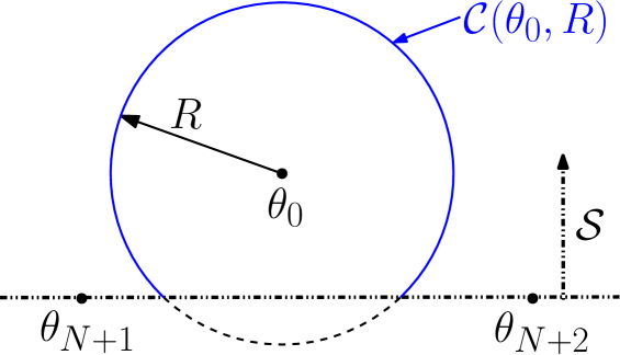
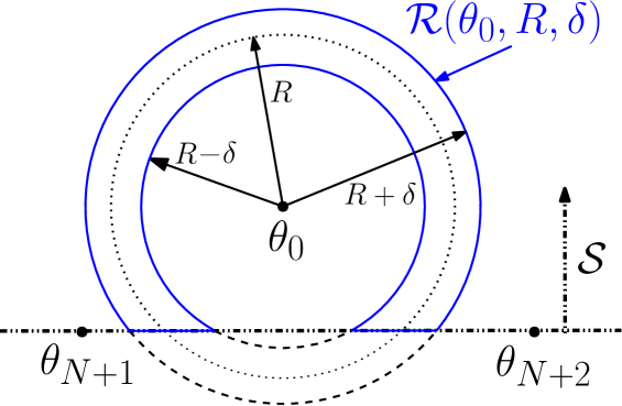
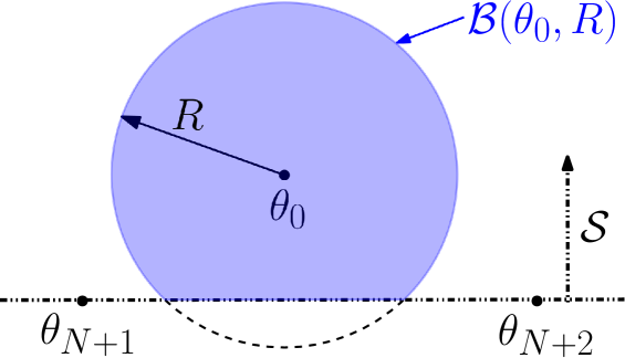
In order to mathematically formulate the attack detector, we first define three geometric shapes. According to Assumption 1, the ROI 𝒜𝒜{\mathcal{A}} is contained in one of the two half spaces produced by dividing the whole space by the line passing through the two secure sensors. We use 𝒮𝒮\mathcal{S} to represent this half space. Let 𝒞(𝜽0,R)𝒞subscript𝜽0𝑅\mathcal{C}({\bm{\theta}}_{0},R) denote the intersection of 𝒮𝒮\cal S and the circle centered at 𝜽0subscript𝜽0{\bm{\theta}}_{0} and with radius R𝑅R, i.e.,

𝒞(𝜽0,R){𝜽𝒮|𝜽𝜽0=R},𝒞subscript𝜽0𝑅conditional-set𝜽𝒮norm𝜽subscript𝜽0𝑅\mathcal{C}({\bm{\theta}}_{0},R)\triangleq\left\{{\bm{\theta}}\in\mathcal{S}\left|\|{\bm{\theta}}-{\bm{\theta}}_{0}\|=R\right.\right\}, (29)

which is illustrated by the blue curve in Fig. 6. Let (𝜽0,R,δ)subscript𝜽0𝑅𝛿\mathcal{R}({\bm{\theta}}_{0},R,\delta) denote the intersection of 𝒮𝒮\cal S and the ring centered at 𝜽0subscript𝜽0{\bm{\theta}}_{0}, with radius R𝑅R and width δ𝛿\delta, i.e.,

(𝜽0,R,δ){𝜽𝒮|Rδ𝜽𝜽0R+δ}.subscript𝜽0𝑅𝛿conditional-set𝜽𝒮𝑅𝛿norm𝜽subscript𝜽0𝑅𝛿\mathcal{R}({\bm{\theta}}_{0},R,\delta)\triangleq\left\{{\bm{\theta}}\in\mathcal{S}\left|R-\delta\leq\|{\bm{\theta}}-{\bm{\theta}}_{0}\|\leq R+\delta\right.\right\}. (30)

The region enclosed by the blue boundary in Fig. 6 depicts an example of (𝜽0,R,δ)subscript𝜽0𝑅𝛿\mathcal{R}({\bm{\theta}}_{0},R,\delta). Let (𝜽0,R)subscript𝜽0𝑅\mathcal{B}({\bm{\theta}}_{0},R) denote the intersection of 𝒮𝒮\cal S and the ball centered at 𝜽0subscript𝜽0{\bm{\theta}}_{0} and with radius R𝑅R, i.e.,

(𝜽0,R){𝜽𝒮|𝜽𝜽0R}.subscript𝜽0𝑅conditional-set𝜽𝒮norm𝜽subscript𝜽0𝑅\mathcal{B}({\bm{\theta}}_{0},R)\triangleq\left\{{\bm{\theta}}\in\mathcal{S}\left|\|{\bm{\theta}}-{\bm{\theta}}_{0}\|\leq R\right.\right\}. (31)

which is the blue region in Fig. 6.

Refer to caption
Figure 4: Geometric illustration of 𝒞(𝜽0,R)𝒞subscript𝜽0𝑅\mathcal{C}({\bm{\theta}}_{0},R).
Refer to caption
Figure 5: Geometric illustration of (𝜽0,R,δ)subscript𝜽0𝑅𝛿\mathcal{R}({\bm{\theta}}_{0},R,\delta).
Refer to caption
Figure 6: Geometric illustration of (𝜽0,R)subscript𝜽0𝑅\mathcal{B}({\bm{\theta}}_{0},R).

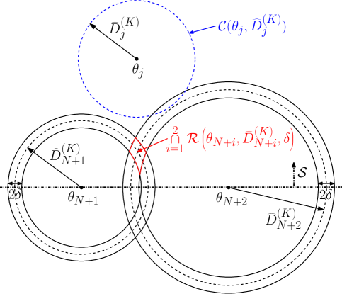
It is worth mentioning that even though j𝒰𝑗𝒰j\in\mathcal{U}, due to the estimation error with finite K𝐾K, the three circles centered at the j𝑗j-th, (N+1)𝑁1(N+1)-th and (N+2)𝑁2(N+2)-th sensors and with radii D^j(K)superscriptsubscript^𝐷𝑗𝐾\widehat{D}_{j}^{(K)}, D^N+1(K)superscriptsubscript^𝐷𝑁1𝐾\widehat{D}_{N+1}^{(K)} and D^N+2(K)superscriptsubscript^𝐷𝑁2𝐾\widehat{D}_{N+2}^{(K)}, respectively, typically will not intersect at a common point. Thus, for finite K𝐾K, checking the geometric inconsistency among 𝒞(𝜽j,D^j(K))𝒞subscript𝜽𝑗superscriptsubscript^𝐷𝑗𝐾\mathcal{C}({\bm{\theta}}_{j},\widehat{D}_{j}^{(K)}), 𝒞(𝜽N+1,D^N+1(K))𝒞subscript𝜽𝑁1superscriptsubscript^𝐷𝑁1𝐾\mathcal{C}({\bm{\theta}}_{N+1},\widehat{D}_{N+1}^{(K)}) and 𝒞(𝜽N+2,D^N+2(K))𝒞subscript𝜽𝑁2superscriptsubscript^𝐷𝑁2𝐾\mathcal{C}({\bm{\theta}}_{N+2},\widehat{D}_{N+2}^{(K)}) cannot reliably tell whether the j𝑗j-th sensor is unattacked or not. To overcome this, we replace 𝒞(𝜽N+1,D^N+1(K))𝒞subscript𝜽𝑁1superscriptsubscript^𝐷𝑁1𝐾\mathcal{C}({\bm{\theta}}_{N+1},\widehat{D}_{N+1}^{(K)}) and 𝒞(𝜽N+2,D^N+2(K))𝒞subscript𝜽𝑁2superscriptsubscript^𝐷𝑁2𝐾\mathcal{C}({\bm{\theta}}_{N+2},\widehat{D}_{N+2}^{(K)}) with (𝜽N+1,D^N+1(K),δ)subscript𝜽𝑁1superscriptsubscript^𝐷𝑁1𝐾𝛿\mathcal{R}({\bm{\theta}}_{N+1},\widehat{D}_{N+1}^{(K)},\delta) and (𝜽N+2,D^N+2(K),δ)subscript𝜽𝑁2superscriptsubscript^𝐷𝑁2𝐾𝛿\mathcal{R}({\bm{\theta}}_{N+2},\widehat{D}_{N+2}^{(K)},\delta) for some δ𝛿\delta, respectively, and scrutinize whether 𝒞(𝜽j,D^j(K))𝒞subscript𝜽𝑗superscriptsubscript^𝐷𝑗𝐾\mathcal{C}({\bm{\theta}}_{j},\widehat{D}_{j}^{(K)}) pass through the common area of (𝜽N+1,D^N+1(K),δ)subscript𝜽𝑁1superscriptsubscript^𝐷𝑁1𝐾𝛿\mathcal{R}({\bm{\theta}}_{N+1},\widehat{D}_{N+1}^{(K)},\delta) and (𝜽N+2,D^N+2(K),δ)subscript𝜽𝑁2superscriptsubscript^𝐷𝑁2𝐾𝛿\mathcal{R}({\bm{\theta}}_{N+2},\widehat{D}_{N+2}^{(K)},\delta) instead.

To be specific, for the j𝑗j-th sensor, j=1,2,,N𝑗12𝑁j=1,2,...,N, we consider the following hypothesis testing problem

{0:j𝒰1:j𝒱cases:subscript0𝑗𝒰:subscript1𝑗𝒱\left\{\begin{array}[]{l}{{\cal{H}}_{0}}:j\in\cal U\\ {{\cal{H}}_{1}}:j\in\cal V\\ \end{array}\right. (32)

and a class of detectors

ϖj(δ)={0, if 𝒞(𝜽j,D^j(K))[i=12(𝜽N+i,D^N+i(K),δ)],1, if 𝒞(𝜽j,D^j(K))[i=12(𝜽N+i,D^N+i(K),δ)]=,\varpi_{j}\left(\delta\right)=\left\{\begin{split}0,&\quad\text{ if }{\mathcal{C}}\left({\bm{\theta}}_{j},\widehat{D}_{j}^{(K)}\right)\cap\left[{\mathop{\cap}\limits_{i=1}^{2}{\cal R}\left({{{\bm{\theta}}_{N+i}},\widehat{D}_{N+i}^{(K)}},\delta\right)}\right]\neq\emptyset,\\ 1,&\quad\text{ if }{\mathcal{C}}\left({\bm{\theta}}_{j},\widehat{D}_{j}^{(K)}\right)\cap\left[{\mathop{\cap}\limits_{i=1}^{2}{\cal R}\left({{{\bm{\theta}}_{N+i}},\widehat{D}_{N+i}^{(K)}},\delta\right)}\right]=\emptyset,\end{split}\right. (33)

for some constant δ𝛿\delta, where D^j(K)superscriptsubscript^𝐷𝑗𝐾\widehat{D}_{j}^{(K)} is defined in (25).

Refer to caption

Figure 7: Geometric illustration of the proposed detectors.

The geometric illustration of the proposed detector in (33) is depicted in Fig. 7, where the region enclosed by the red curves is the common area of (𝜽N+1,D^N+1(K),δ)subscript𝜽𝑁1superscriptsubscript^𝐷𝑁1𝐾𝛿\mathcal{R}({\bm{\theta}}_{N+1},\widehat{D}_{N+1}^{(K)},\delta) and (𝜽N+2,D^N+2(K),δ)subscript𝜽𝑁2superscriptsubscript^𝐷𝑁2𝐾𝛿\mathcal{R}({\bm{\theta}}_{N+2},\widehat{D}_{N+2}^{(K)},\delta) which plays an important role in the attack detection process. It is worth noticing that the center of this common area is determined by two random variables D^N+1(K)superscriptsubscript^𝐷𝑁1𝐾\widehat{D}_{N+1}^{(K)} and D^N+2(K)superscriptsubscript^𝐷𝑁2𝐾\widehat{D}_{N+2}^{(K)}, and thereby is randomly located. To this end, this common area may not cover the true target location 𝜽Tsubscript𝜽T{\bm{\theta}}_{{\rm{T}}}. In addition, the size of the common area of (𝜽N+1,D^N+1(K),δ)subscript𝜽𝑁1superscriptsubscript^𝐷𝑁1𝐾𝛿\mathcal{R}({\bm{\theta}}_{N+1},\widehat{D}_{N+1}^{(K)},\delta) and (𝜽N+2,D^N+2(K),δ)subscript𝜽𝑁2superscriptsubscript^𝐷𝑁2𝐾𝛿\mathcal{R}({\bm{\theta}}_{N+2},\widehat{D}_{N+2}^{(K)},\delta) depends on the parameter δ𝛿\delta which impacts the false alarm and miss probabilities of the proposed detector.

IV Performance Analysis of the Proposed Detector

In this section, the detection performance of the proposed detector in (33) is investigated. We will show that the false alarm and miss probabilities of the proposed detector decay exponentially fast as the number of data samples at each sensor increases.

To start with, we provide the following lemma regarding the lower and upper bounds on the common area of (𝜽N+1,DN+1,δ)subscript𝜽𝑁1subscript𝐷𝑁1𝛿\mathcal{R}({\bm{\theta}}_{N+1},D_{N+1},\delta) and (𝜽N+2,DN+2,δ)subscript𝜽𝑁2subscript𝐷𝑁2𝛿\mathcal{R}({\bm{\theta}}_{N+2},D_{N+2},\delta).

Lemma 1

If

δ<Υmin{Υ1,Υ2},𝛿ΥsubscriptΥ1subscriptΥ2\delta<\Upsilon\triangleq\min\{\Upsilon_{1},\Upsilon_{2}\}, (34)

then

sup𝜽i=12(𝜽N+i,D^N+i(K),δ)𝜽𝜽T<Φ(δ)(2DU+Υ)12[2DU+ΥDS(ΥDS+1)+2]12δ,subscriptsupremum𝜽superscriptsubscript𝑖12subscript𝜽𝑁𝑖superscriptsubscript^𝐷𝑁𝑖𝐾𝛿norm𝜽subscript𝜽TΦ𝛿superscript2subscript𝐷𝑈Υ12superscriptdelimited-[]2subscript𝐷𝑈Υsubscript𝐷𝑆Υsubscript𝐷𝑆1212𝛿\mathop{\sup}\limits_{{\bm{\theta}}\in{\mathop{\cap}\limits_{i=1}^{2}{\cal R}\left({{{\bm{\theta}}_{N+i}},\widehat{D}_{N+i}^{(K)}},\delta\right)}}\left\|{{\bm{\theta}}-{{\bm{\theta}}_{\rm{T}}}}\right\|<\Phi(\delta)\triangleq\left({2{D_{U}}+\Upsilon}\right)^{\frac{1}{2}}\left[{\frac{{2{D_{U}}+\Upsilon}}{{{D_{S}}}}\left({\frac{\Upsilon}{{{D_{S}}}}+1}\right)+2}\right]^{\frac{1}{2}}\sqrt{\delta}, (35)

which implies

(𝜽T,δ)i=12(𝜽N+i,D^N+i(K),δ)(𝜽T,Φ(δ)).subscript𝜽T𝛿superscriptsubscript𝑖12subscript𝜽𝑁𝑖superscriptsubscript^𝐷𝑁𝑖𝐾𝛿subscript𝜽TΦ𝛿\mathcal{B}({\bm{\theta}}_{\rm{T}},\delta)\subseteq{\mathop{\cap}\limits_{i=1}^{2}{\cal R}\left({{{\bm{\theta}}_{N+i}},\widehat{D}_{N+i}^{(K)}},\delta\right)}\subseteq\mathcal{B}\left({\bm{\theta}}_{\rm{T}},\Phi(\delta)\right). (36)
Proof:

Refer to Appendix A. ∎

As demonstrated by Lemma 1, the common area of (𝜽N+1,DN+1,δ)subscript𝜽𝑁1subscript𝐷𝑁1𝛿\mathcal{R}({\bm{\theta}}_{N+1},D_{N+1},\delta) and (𝜽N+2,DN+2,δ)subscript𝜽𝑁2subscript𝐷𝑁2𝛿\mathcal{R}({\bm{\theta}}_{N+2},D_{N+2},\delta) can be bounded by two balls from below and above. Moreover, the radii of these two balls are both increasing functions of the given δ𝛿\delta. It will be shown later that by employing the two balls to approximate the irregular area i=12(𝜽N+i,D^N+i(K),δ)superscriptsubscript𝑖12subscript𝜽𝑁𝑖superscriptsubscript^𝐷𝑁𝑖𝐾𝛿{\cap_{i=1}^{2}{\cal R}({{{\bm{\theta}}_{N+i}},\widehat{D}_{N+i}^{(K)}},\delta)} from below and above, the detection performance analysis of the proposed detector in (33) can be considerably facilitated.

IV-A Upper Bound on False Alarm Probability

From (33), the false alarm and miss probabilities of the proposed detector are given by 0(ϖj(δ)=1)subscript0subscriptitalic-ϖ𝑗𝛿1{\mathbbm{P}_{0}}\left({{\varpi_{j}\left(\delta\right)=1}}\right) and 1(ϖj(δ)=0)subscript1subscriptitalic-ϖ𝑗𝛿0{\mathbbm{P}_{1}}\left({{\varpi_{j}\left(\delta\right)=0}}\right), respectively, where isubscript𝑖\mathbbm{P}_{i} denotes the probability measure under hypothesis isubscript𝑖{\mathcal{H}}_{i}.

Let isubscript𝑖\mathcal{E}_{i} denote the event

i=Δ{|D^N+i(K)DN+i|<12δ},i=1,2,formulae-sequencesuperscriptΔsubscript𝑖superscriptsubscript^𝐷𝑁𝑖𝐾subscript𝐷𝑁𝑖12𝛿𝑖12{\cal E}_{i}\buildrel\Delta\over{=}\left\{{\left|{\widehat{D}_{N+i}^{(K)}-D_{N+i}}\right|<\frac{1}{2}\delta}\right\},\;i=1,2, (37)

and iCsuperscriptsubscript𝑖C{\mathcal{E}_{i}^{\rm{C}}} denotes the complement of the event isubscript𝑖\mathcal{E}_{i}. The false alarm probability of the detector in (33) can be expressed as

0(ϖj(δ)=1)subscript0subscriptitalic-ϖ𝑗𝛿1\displaystyle{\mathbbm{P}_{0}}\left({{\varpi_{j}\left(\delta\right)=1}}\right) =0(𝒞(𝜽j,D^j(K))[i=12(𝜽N+i,D^N+i(K),δ)]=)absentsubscript0𝒞subscript𝜽𝑗superscriptsubscript^𝐷𝑗𝐾delimited-[]superscriptsubscript𝑖12subscript𝜽𝑁𝑖superscriptsubscript^𝐷𝑁𝑖𝐾𝛿\displaystyle={\mathbbm{P}_{0}}\left({{\cal C}\left({{{\bm{\theta}}_{j}},\widehat{D}_{j}^{(K)}}\right)\cap\left[{\mathop{\cap}\limits_{i=1}^{2}{\cal R}\left({{{\bm{\theta}}_{N+i}},\widehat{D}_{N+i}^{(K)}},\delta\right)}\right]=\emptyset}\right)
=0({𝒞(𝜽j,D^j(K))[i=12(𝜽N+i,D^N+i(K),δ)]=}(12))absentsubscript0𝒞subscript𝜽𝑗superscriptsubscript^𝐷𝑗𝐾delimited-[]superscriptsubscript𝑖12subscript𝜽𝑁𝑖superscriptsubscript^𝐷𝑁𝑖𝐾𝛿subscript1subscript2\displaystyle={\mathbbm{P}_{0}}\left({\left\{{\cal C}\left({{{\bm{\theta}}_{j}},\widehat{D}_{j}^{(K)}}\right)\cap\left[{\mathop{\cap}\limits_{i=1}^{2}{\cal R}\left({{{\bm{\theta}}_{N+i}},\widehat{D}_{N+i}^{(K)}},\delta\right)}\right]=\emptyset\right\}\cap\left(\mathcal{E}_{1}\cap\mathcal{E}_{2}\right)}\right)
+0({𝒞(𝜽j,D^j(K))[i=12(𝜽N+i,D^N+i(K),δ)]=}(1C2C)).subscript0𝒞subscript𝜽𝑗superscriptsubscript^𝐷𝑗𝐾delimited-[]superscriptsubscript𝑖12subscript𝜽𝑁𝑖superscriptsubscript^𝐷𝑁𝑖𝐾𝛿superscriptsubscript1Csuperscriptsubscript2C\displaystyle\quad+{\mathbbm{P}_{0}}\left({\left\{{\cal C}\left({{{\bm{\theta}}_{j}},\widehat{D}_{j}^{(K)}}\right)\cap\left[{\mathop{\cap}\limits_{i=1}^{2}{\cal R}\left({{{\bm{\theta}}_{N+i}},\widehat{D}_{N+i}^{(K)}},\delta\right)}\right]=\emptyset\right\}\cap\left({\mathcal{E}_{1}^{\rm{C}}}\cup{\mathcal{E}_{2}^{\rm{C}}}\right)}\right). (38)

Note that isubscript𝑖{\cal E}_{i} implies that

(𝜽N+i,DN+i,12δ)(𝜽N+i,D^N+i(K),δ),subscript𝜽𝑁𝑖subscript𝐷𝑁𝑖12𝛿subscript𝜽𝑁𝑖superscriptsubscript^𝐷𝑁𝑖𝐾𝛿\mathcal{R}\left({\bm{\theta}}_{N+i},D_{N+i},\frac{1}{2}\delta\right)\subseteq\mathcal{R}\left({\bm{\theta}}_{N+i},\widehat{D}_{N+i}^{(K)},\delta\right), (39)

and hence, from (38), we can obtain

0(ϖj(δ)=1)subscript0subscriptitalic-ϖ𝑗𝛿1\displaystyle{\mathbbm{P}_{0}}\left({{\varpi_{j}\left(\delta\right)=1}}\right) 0({𝒞(𝜽j,D^j(K))[i=12(𝜽N+i,DN+i,12δ)]=}(12))absentsubscript0𝒞subscript𝜽𝑗superscriptsubscript^𝐷𝑗𝐾delimited-[]superscriptsubscript𝑖12subscript𝜽𝑁𝑖subscript𝐷𝑁𝑖12𝛿subscript1subscript2\displaystyle\leq{\mathbbm{P}_{0}}\left({\left\{{{\cal C}\left({{{\bm{\theta}}_{j}},\widehat{D}_{j}^{(K)}}\right)\cap\left[{\mathop{\cap}\limits_{i=1}^{2}{\cal R}\left({{{\bm{\theta}}_{N+i}},{D_{N+i}},\frac{1}{2}\delta}\right)}\right]=\emptyset}\right\}\cap\left({{{\cal E}_{1}}\cap{{\cal E}_{2}}}\right)}\right)
+0({𝒞(𝜽j,D^j(K))[i=12(𝜽N+i,D^N+i(K),δ)]=}(1C2C))subscript0𝒞subscript𝜽𝑗superscriptsubscript^𝐷𝑗𝐾delimited-[]superscriptsubscript𝑖12subscript𝜽𝑁𝑖superscriptsubscript^𝐷𝑁𝑖𝐾𝛿superscriptsubscript1Csuperscriptsubscript2C\displaystyle\quad+{\mathbbm{P}_{0}}\left({\left\{{{\cal C}\left({{{\bm{\theta}}_{j}},\widehat{D}_{j}^{(K)}}\right)\cap\left[{\mathop{\cap}\limits_{i=1}^{2}{\cal R}\left({{{\bm{\theta}}_{N+i}},\widehat{D}_{N+i}^{(K)},\delta}\right)}\right]=\emptyset}\right\}\cap\left({{\cal E}_{1}^{\rm{C}}\cup{\cal E}_{2}^{\rm{C}}}\right)}\right)
0(𝒞(𝜽j,D^j(K))[i=12(𝜽N+i,DN+i,12δ)]=)+0(1C2C)absentsubscript0𝒞subscript𝜽𝑗superscriptsubscript^𝐷𝑗𝐾delimited-[]superscriptsubscript𝑖12subscript𝜽𝑁𝑖subscript𝐷𝑁𝑖12𝛿subscript0superscriptsubscript1Csuperscriptsubscript2C\displaystyle\leq{\mathbbm{P}_{0}}\left({{\cal C}\left({{{\bm{\theta}}_{j}},\widehat{D}_{j}^{(K)}}\right)\cap\left[{\mathop{\cap}\limits_{i=1}^{2}{\cal R}\left({{{\bm{\theta}}_{N+i}},{D_{N+i}},\frac{1}{2}\delta}\right)}\right]=\emptyset}\right)+{\mathbbm{P}_{0}}\left({{\cal E}_{1}^{\rm{C}}\cup{\cal E}_{2}^{\rm{C}}}\right) (40)
0(𝒞(𝜽j,D^j(K))[i=12(𝜽N+i,DN+i,12δ)]=)+0(1C)+0(2C),absentsubscript0𝒞subscript𝜽𝑗superscriptsubscript^𝐷𝑗𝐾delimited-[]superscriptsubscript𝑖12subscript𝜽𝑁𝑖subscript𝐷𝑁𝑖12𝛿subscript0superscriptsubscript1Csubscript0superscriptsubscript2C\displaystyle\leq{\mathbbm{P}_{0}}\left({{\cal C}\left({{{\bm{\theta}}_{j}},\widehat{D}_{j}^{(K)}}\right)\cap\left[{\mathop{\cap}\limits_{i=1}^{2}{\cal R}\left({{{\bm{\theta}}_{N+i}},{D_{N+i}},\frac{1}{2}\delta}\right)}\right]\!=\!\emptyset}\right)\!+\!{\mathbbm{P}_{0}}\left({{\cal E}_{1}^{\rm{C}}}\right)\!+\!{\mathbbm{P}_{0}}\left({{\cal E}_{2}^{\rm{C}}}\right), (41)

where (40) is due to the fact that 0()0()subscript0subscript0{\mathbbm{P}}_{0}({\cal E}\cap{\cal F})\leq{\mathbbm{P}}_{0}({\cal E}) for any two events \cal E and \cal F. Moreover, from Lemma 1, we know

(𝜽T,12δ)i=12(𝜽N+i,DN+i,12δ),subscript𝜽T12𝛿superscriptsubscript𝑖12subscript𝜽𝑁𝑖subscript𝐷𝑁𝑖12𝛿\mathcal{B}\left({\bm{\theta}}_{\rm{T}},\frac{1}{2}\delta\right)\subseteq{\mathop{\cap}\limits_{i=1}^{2}{\cal R}\left({{{\bm{\theta}}_{N+i}},{D_{N+i}},\frac{1}{2}\delta}\right)}, (42)

which yields

0(ϖj(δ)=1)0(𝒞(𝜽j,D^j(K))(𝜽T,12δ)=)+0(1C)+0(2C).subscript0subscriptitalic-ϖ𝑗𝛿1subscript0𝒞subscript𝜽𝑗superscriptsubscript^𝐷𝑗𝐾subscript𝜽T12𝛿subscript0superscriptsubscript1Csubscript0superscriptsubscript2C{\mathbbm{P}_{0}}\left({{\varpi_{j}\left(\delta\right)=1}}\right)\leq{\mathbbm{P}_{0}}\left({{\cal C}\left({{{\bm{\theta}}_{j}},\widehat{D}_{j}^{(K)}}\right)\cap\mathcal{B}\left({\bm{\theta}}_{\rm{T}},\frac{1}{2}\delta\right)=\emptyset}\right)+{\mathbbm{P}_{0}}\left({{\cal E}_{1}^{\rm{C}}}\right)+{\mathbbm{P}_{0}}\left({{\cal E}_{2}^{\rm{C}}}\right). (43)

Refer to caption

Figure 8: Geometric illustration of (44).

In addition, as illustrated in Fig. 8, if j𝒰𝑗𝒰j\in\mathcal{U}, we know 𝜽T𝒞(𝜽j,Dj)subscript𝜽T𝒞subscript𝜽𝑗subscript𝐷𝑗{\bm{\theta}}_{\rm T}\in{\cal C}({{{\bm{\theta}}_{j}},D_{j}}) which yields that under hypothesis 0subscript0\mathcal{H}_{0},

{𝒞(𝜽j,D^j(K))(𝜽T,12δ)=}{|D^j(K)Dj|12δ},𝒞subscript𝜽𝑗superscriptsubscript^𝐷𝑗𝐾subscript𝜽T12𝛿superscriptsubscript^𝐷𝑗𝐾subscript𝐷𝑗12𝛿\left\{{{\cal C}\left({{{\bm{\theta}}_{j}},\widehat{D}_{j}^{(K)}}\right)\cap{\cal B}\left({{{\bm{\theta}}_{\rm{T}}},\frac{1}{2}\delta}\right)=\emptyset}\right\}\Leftrightarrow\left\{{\left|{\widehat{D}_{j}^{(K)}-{D_{j}}}\right|\geq\frac{1}{2}\delta}\right\}, (44)

and therefore, by employing (37) and (43), the false alarm probability can be bounded from above as per

0(ϖj(δ)=1)subscript0subscriptitalic-ϖ𝑗𝛿1\displaystyle{\mathbbm{P}_{0}}\left({{\varpi_{j}\left(\delta\right)=1}}\right) 0(|D^j(K)Dj|12δ)+0(1C)+0(2C)absentsubscript0superscriptsubscript^𝐷𝑗𝐾subscript𝐷𝑗12𝛿subscript0superscriptsubscript1Csubscript0superscriptsubscript2C\displaystyle\leq{\mathbbm{P}_{0}}\left({\left|{\widehat{D}_{j}^{(K)}-{D_{j}}}\right|\geq\frac{1}{2}\delta}\right)+{\mathbbm{P}_{0}}\left({{\cal E}_{1}^{\rm{C}}}\right)+{\mathbbm{P}_{0}}\left({{\cal E}_{2}^{\rm{C}}}\right)
=0(|D^j(K)Dj|12δ)+i=120(|D^N+i(K)DN+i|12δ).absentsubscript0superscriptsubscript^𝐷𝑗𝐾subscript𝐷𝑗12𝛿superscriptsubscript𝑖12subscript0superscriptsubscript^𝐷𝑁𝑖𝐾subscript𝐷𝑁𝑖12𝛿\displaystyle={\mathbbm{P}_{0}}\left({\left|{\widehat{D}_{j}^{(K)}-{D_{j}}}\right|\geq\frac{1}{2}\delta}\right)+\sum\limits_{i=1}^{2}{{\mathbbm{P}_{0}}\left({\left|{\widehat{D}_{N+i}^{(K)}-{D_{N+i}}}\right|\geq\frac{1}{2}\delta}\right)}. (45)

IV-B Upper Bound on Miss Probability

On the other hand, the miss probability of the detector in (33) can be bounded from above as per

1(ϖj(δ)=0)subscript1subscriptitalic-ϖ𝑗𝛿0\displaystyle{\mathbbm{P}_{1}}\left({{\varpi_{j}\left(\delta\right)=0}}\right) =1(𝒞(𝜽j,D^j(K))[i=12(𝜽N+i,D^N+i(K),δ)])absentsubscript1𝒞subscript𝜽𝑗superscriptsubscript^𝐷𝑗𝐾delimited-[]superscriptsubscript𝑖12subscript𝜽𝑁𝑖superscriptsubscript^𝐷𝑁𝑖𝐾𝛿\displaystyle={\mathbbm{P}_{1}}\left({{\cal C}\left({{{\bm{\theta}}_{j}},\widehat{D}_{j}^{(K)}}\right)\cap\left[{\mathop{\cap}\limits_{i=1}^{2}{\cal R}\left({{{\bm{\theta}}_{N+i}},\widehat{D}_{N+i}^{(K)},\delta}\right)}\right]\neq\emptyset}\right)
=1({𝒞(𝜽j,D^j(K))[i=12(𝜽N+i,D^N+i(K),δ)]}(12))absentsubscript1𝒞subscript𝜽𝑗superscriptsubscript^𝐷𝑗𝐾delimited-[]superscriptsubscript𝑖12subscript𝜽𝑁𝑖superscriptsubscript^𝐷𝑁𝑖𝐾𝛿subscript1subscript2\displaystyle={\mathbbm{P}_{1}}\left({\left\{{{\cal C}\left({{{\bm{\theta}}_{j}},\widehat{D}_{j}^{(K)}}\right)\cap\left[{\mathop{\cap}\limits_{i=1}^{2}{\cal R}\left({{{\bm{\theta}}_{N+i}},\widehat{D}_{N+i}^{(K)},\delta}\right)}\right]\neq\emptyset}\right\}\cap\left({{{\cal E}_{1}}\cap{{\cal E}_{2}}}\right)}\right)
+1({𝒞(𝜽j,D^j(K))[i=12(𝜽N+i,D^N+i(K),δ)]}(1C2C))subscript1𝒞subscript𝜽𝑗superscriptsubscript^𝐷𝑗𝐾delimited-[]superscriptsubscript𝑖12subscript𝜽𝑁𝑖superscriptsubscript^𝐷𝑁𝑖𝐾𝛿superscriptsubscript1Csuperscriptsubscript2C\displaystyle\quad+{\mathbbm{P}_{1}}\left({\left\{{{\cal C}\left({{{\bm{\theta}}_{j}},\widehat{D}_{j}^{(K)}}\right)\cap\left[{\mathop{\cap}\limits_{i=1}^{2}{\cal R}\left({{{\bm{\theta}}_{N+i}},\widehat{D}_{N+i}^{(K)},\delta}\right)}\right]\neq\emptyset}\right\}\cap\left({{\cal E}_{1}^{\rm{C}}\cup{\cal E}_{2}^{\rm{C}}}\right)}\right)
1({𝒞(𝜽j,D^j(K))[i=12(𝜽N+i,DN+i,32δ)]}(12))absentsubscript1𝒞subscript𝜽𝑗superscriptsubscript^𝐷𝑗𝐾delimited-[]superscriptsubscript𝑖12subscript𝜽𝑁𝑖subscript𝐷𝑁𝑖32𝛿subscript1subscript2\displaystyle\leq{\mathbbm{P}_{1}}\left({\left\{{{\cal C}\left({{{\bm{\theta}}_{j}},\widehat{D}_{j}^{(K)}}\right)\cap\left[{\mathop{\cap}\limits_{i=1}^{2}{\cal R}\left({{{\bm{\theta}}_{N+i}},{D_{N+i}},\frac{3}{2}\delta}\right)}\right]\neq\emptyset}\right\}\cap\left({{{\cal E}_{1}}\cap{{\cal E}_{2}}}\right)}\right)
+1(1C2C)subscript1superscriptsubscript1Csuperscriptsubscript2C\displaystyle\quad+{\mathbbm{P}_{1}}\left({{\cal E}_{1}^{\rm{C}}\cup{\cal E}_{2}^{\rm{C}}}\right) (46)
1(𝒞(𝜽j,D^j(K))[i=12(𝜽N+i,DN+i,32δ)])+1(1C)+1(2C)absentsubscript1𝒞subscript𝜽𝑗superscriptsubscript^𝐷𝑗𝐾delimited-[]superscriptsubscript𝑖12subscript𝜽𝑁𝑖subscript𝐷𝑁𝑖32𝛿subscript1superscriptsubscript1Csubscript1superscriptsubscript2C\displaystyle\leq{\mathbbm{P}_{1}}\left({{\cal C}\left({{{\bm{\theta}}_{j}},\widehat{D}_{j}^{(K)}}\right)\cap\left[{\mathop{\cap}\limits_{i=1}^{2}{\cal R}\left({{{\bm{\theta}}_{N+i}},{D_{N+i}},\frac{3}{2}\delta}\right)}\right]\neq\emptyset}\right)+{\mathbbm{P}_{1}}\left({{\cal E}_{1}^{\rm{C}}}\right)+{\mathbbm{P}_{1}}\left({{\cal E}_{2}^{\rm{C}}}\right)
1(𝒞(𝜽j,D^j(K))(𝜽T,Φ(32δ)))+1(1C)+1(2C),absentsubscript1𝒞subscript𝜽𝑗superscriptsubscript^𝐷𝑗𝐾subscript𝜽TΦ32𝛿subscript1superscriptsubscript1Csubscript1superscriptsubscript2C\displaystyle\leq{\mathbbm{P}_{1}}\left({{\cal C}\left({{{\bm{\theta}}_{j}},\widehat{D}_{j}^{(K)}}\right)\cap{\cal B}\left({{{\bm{\theta}}_{\rm{T}}},\Phi\left({\frac{3}{2}\delta}\right)}\right)\neq\emptyset}\right)+{\mathbbm{P}_{1}}\left({{\cal E}_{1}^{\rm{C}}}\right)+{\mathbbm{P}_{1}}\left({{\cal E}_{2}^{\rm{C}}}\right), (47)

where (46) is due to the fact that if 1subscript1\mathcal{E}_{1} and 2subscript2\mathcal{E}_{2} occur, then

(𝜽N+i,D^N+i(K),δ)(𝜽N+i,DN+i,32δ),i=1,2,formulae-sequencesubscript𝜽𝑁𝑖superscriptsubscript^𝐷𝑁𝑖𝐾𝛿subscript𝜽𝑁𝑖subscript𝐷𝑁𝑖32𝛿𝑖12{\cal R}\left({{{\bm{\theta}}_{N+i}},\widehat{D}_{N+i}^{(K)},\delta}\right)\subseteq{\cal R}\left({{{\bm{\theta}}_{N+i}},D_{N+i},\frac{3}{2}\delta}\right),\;i=1,2, (48)

and (47) is because i=12(𝜽N+i,DN+i,32δ)(𝜽T,Φ(32δ))superscriptsubscript𝑖12subscript𝜽𝑁𝑖subscript𝐷𝑁𝑖32𝛿subscript𝜽TΦ32𝛿{\cap_{i=1}^{2}{\cal R}\left({{{\bm{\theta}}_{N+i}},{D_{N+i}},\frac{3}{2}\delta}\right)}\subseteq{\cal B}\left({{{\bm{\theta}}_{\rm{T}}},\Phi\left({\frac{3}{2}\delta}\right)}\right) according to Lemma 1.

Since the first term in (47) is hard to deal with, we employ an upper bound on it which is provided in the following lemma.

Lemma 2

Define

λjκD0P01γ[τjFj1(ρj(L))]γ+1γsupx[Fj1(ρj(L)),Fj1(ρj(U))]fj(x),subscript𝜆𝑗𝜅subscript𝐷0superscriptsubscript𝑃01𝛾superscriptdelimited-[]subscript𝜏𝑗superscriptsubscript𝐹𝑗1superscriptsubscript𝜌𝑗L𝛾1𝛾subscriptsupremum𝑥superscriptsubscript𝐹𝑗1superscriptsubscript𝜌𝑗Lsuperscriptsubscript𝐹𝑗1superscriptsubscript𝜌𝑗Usubscript𝑓𝑗𝑥\lambda_{j}\triangleq\frac{\kappa{{D_{0}}P_{0}^{\frac{1}{\gamma}}{{\left[{{\tau_{j}}-F_{j}^{-1}\left({{\rho_{j}^{(\rm{L})}}}\right)}\right]}^{-\frac{{\gamma+1}}{\gamma}}}}}{{\mathop{\sup}\limits_{x\in\left[{{F_{j}^{-1}(\rho_{j}^{(\rm{L})})},{F_{j}^{-1}(\rho_{j}^{(\rm{U})})}}\right]}{f_{j}}\left(x\right)}}, (49)

and denote

λ=minj=1,2,,N{λj}.𝜆subscript𝑗12𝑁subscript𝜆𝑗\lambda=\mathop{\min}\limits_{j=1,2,...,N}\left\{{{\lambda_{j}}}\right\}. (50)

If

0<δ<min{Υ,{(2DU+Υ)12[6DU+3Υ2DS(ΥDS+1)+3]12+12Υ12}2λ2},0𝛿Υsuperscriptsuperscript2subscript𝐷𝑈Υ12superscriptdelimited-[]6subscript𝐷𝑈3Υ2subscript𝐷𝑆Υsubscript𝐷𝑆131212superscriptΥ122superscript𝜆20<\delta<\min{\left\{{\Upsilon,\left\{{{{\left({2{D_{U}}+\Upsilon}\right)}^{\frac{1}{2}}}{{\left[{\frac{{6{D_{U}}+3\Upsilon}}{{2{D_{S}}}}\left({\frac{\Upsilon}{{{D_{S}}}}+1}\right)+3}\right]}^{\frac{1}{2}}}+{\frac{1}{2}\Upsilon^{\frac{1}{2}}}}\right\}^{-2}{\lambda^{2}}}\right\}}, (51)

then

1(𝒞(𝜽j,D^j(K))(𝜽T,Φ(32δ)))1(|D^j(K)D~j|12δ),subscript1𝒞subscript𝜽𝑗superscriptsubscript^𝐷𝑗𝐾subscript𝜽TΦ32𝛿subscript1superscriptsubscript^𝐷𝑗𝐾subscript~𝐷𝑗12𝛿{\mathbbm{P}_{1}}\left({{\cal C}\left({{{\bm{\theta}}_{j}},\widehat{D}_{j}^{(K)}}\right)\cap{\cal B}\left({{{\bm{\theta}}_{\rm{T}}},\Phi\left({\frac{3}{2}\delta}\right)}\right)\neq\emptyset}\right)\leq{\mathbbm{P}_{1}}\left({\left|{\widehat{D}_{j}^{(K)}-{{\widetilde{D}}_{j}}}\right|\geq\frac{1}{2}\delta}\right), (52)

where D~jsubscript~𝐷𝑗{{\widetilde{D}}_{j}} is defined in (27).

Proof:

Refer to Appendix B. ∎

It is worth mentioning that since fj(x)subscript𝑓𝑗𝑥f_{j}(x) is continuous and positive over {x|Fj(x)(0,1)}conditional-set𝑥subscript𝐹𝑗𝑥01\{x|F_{j}(x)\in(0,1)\}, the denominator supx[Fj1(ρj(L)),Fj1(ρj(U))]fj(x)subscriptsupremum𝑥superscriptsubscript𝐹𝑗1superscriptsubscript𝜌𝑗Lsuperscriptsubscript𝐹𝑗1superscriptsubscript𝜌𝑗Usubscript𝑓𝑗𝑥{{\sup}_{x\in\left[{{F_{j}^{-1}(\rho_{j}^{(\rm{L})})},{F_{j}^{-1}(\rho_{j}^{(\rm{U})})}}\right]}{f_{j}}\left(x\right)} in (49) is positive and bounded. Moreover, according to (10), we know that τj>Fj1(ρj(L))subscript𝜏𝑗superscriptsubscript𝐹𝑗1superscriptsubscript𝜌𝑗L\tau_{j}>F_{j}^{-1}(\rho_{j}^{(\rm{L})}), since Fj1superscriptsubscript𝐹𝑗1F_{j}^{-1} is strictly increasing. Therefore, 0<λj<0subscript𝜆𝑗0<\lambda_{j}<\infty, and hence, 0<λ<0𝜆0<\lambda<\infty.

By employing (47) and Lemma 2, we know if (51) holds, then an upper bound on the miss probability of the detector in (33) can be expressed as

1(ϖj(δ)=0)subscript1subscriptitalic-ϖ𝑗𝛿0\displaystyle{\mathbbm{P}_{1}}\left({{\varpi_{j}\left(\delta\right)=0}}\right) 1(|D^j(K)D~j|12δ)+1(1C)+1(2C)absentsubscript1superscriptsubscript^𝐷𝑗𝐾subscript~𝐷𝑗12𝛿subscript1superscriptsubscript1Csubscript1superscriptsubscript2C\displaystyle\leq{\mathbbm{P}_{1}}\left({\left|{\widehat{D}_{j}^{(K)}-{{\widetilde{D}}_{j}}}\right|\geq\frac{1}{2}\delta}\right)+{\mathbbm{P}_{1}}\left({{\cal E}_{1}^{\rm{C}}}\right)+{\mathbbm{P}_{1}}\left({{\cal E}_{2}^{\rm{C}}}\right)
=1(|D^j(K)D~j|12δ)+i=121(|D^N+i(K)DN+i|12δ).absentsubscript1superscriptsubscript^𝐷𝑗𝐾subscript~𝐷𝑗12𝛿superscriptsubscript𝑖12subscript1superscriptsubscript^𝐷𝑁𝑖𝐾subscript𝐷𝑁𝑖12𝛿\displaystyle={\mathbbm{P}_{1}}\left({\left|{\widehat{D}_{j}^{(K)}-{{\widetilde{D}}_{j}}}\right|\geq\frac{1}{2}\delta}\right)+\sum\limits_{i=1}^{2}{{\mathbbm{P}_{1}}\left({\left|{\widehat{D}_{N+i}^{(K)}-{D_{N+i}}}\right|\geq\frac{1}{2}\delta}\right)}. (53)

IV-C Exponential Decay of False Alarm and Miss Probabilities

It is seen from (45) and (53) that the upper bounds on the false alarm and miss probabilities have some similarities. To be specific, since the (N+1)𝑁1(N+1)-th and (N+2)𝑁2(N+2)-th sensors are secure, 0(|D^N+i(K)DN+i|12δ)=1(|D^N+i(K)DN+i|12δ)subscript0superscriptsubscript^𝐷𝑁𝑖𝐾subscript𝐷𝑁𝑖12𝛿subscript1superscriptsubscript^𝐷𝑁𝑖𝐾subscript𝐷𝑁𝑖12𝛿{{\mathbbm{P}_{0}}\left({\left|{\widehat{D}_{N+i}^{(K)}-{D_{N+i}}}\right|\geq\frac{1}{2}\delta}\right)}={{\mathbbm{P}_{1}}\left({\left|{\widehat{D}_{N+i}^{(K)}-{D_{N+i}}}\right|\geq\frac{1}{2}\delta}\right)} for i=1,2𝑖12i=1,2. Thus, the second term in (45) is the same as the second term in (53). Moreover, as K𝐾K\to\infty, D^j(K)Djsuperscriptsubscript^𝐷𝑗𝐾subscript𝐷𝑗\widehat{D}_{j}^{(K)}\to D_{j} almost surely under hypothesis 0subscript0\mathcal{H}_{0}, while D^j(K)D~jsuperscriptsubscript^𝐷𝑗𝐾subscript~𝐷𝑗\widehat{D}_{j}^{(K)}\to\widetilde{D}_{j} almost surely under hypothesis 1subscript1\mathcal{H}_{1}, one can expect that the first term in (45) and the first term in (53) behave in a very similar way as K𝐾K increases, except for the change in D^j(K)superscriptsubscript^𝐷𝑗𝐾\widehat{D}_{j}^{(K)} due to the attack. In the following theorem, by employing (45) and (53), we show that the false alarm and miss probabilities of the detector in (33) decay at least exponentially with respect to K𝐾K.

Theorem 1

If (51) holds, then the false alarm and miss probabilities are upper bounded by

0(ϖj(δ)=1)12eηj(0)(δ)K,subscript0subscriptitalic-ϖ𝑗𝛿112superscript𝑒superscriptsubscript𝜂𝑗0𝛿𝐾{\mathbbm{P}_{0}}\left({{\varpi_{j}\left(\delta\right)=1}}\right)\leq 12{e^{-\eta_{j}^{({0})}\left(\delta\right)K}}, (54)
1(ϖj(δ)=0)12eηj(1)(δ)K,subscript1subscriptitalic-ϖ𝑗𝛿012superscript𝑒superscriptsubscript𝜂𝑗1𝛿𝐾{\mathbbm{P}_{1}}\left({{\varpi_{j}\left(\delta\right)=0}}\right)\leq 12{e^{-\eta_{j}^{({1})}\left(\delta\right)K}}, (55)

for some positive constants ηj(0)(δ)superscriptsubscript𝜂𝑗0𝛿\eta_{j}^{(0)}\left(\delta\right) and ηj(1)(δ)superscriptsubscript𝜂𝑗1𝛿\eta_{j}^{(1)}\left(\delta\right).

Proof:

Before proceeding, we define a sequence of events j,Ksubscript𝑗𝐾\mathcal{F}_{j,K} as

j,K{ξj(K)[εj(L),εj(U)]},subscript𝑗𝐾superscriptsubscript𝜉𝑗𝐾superscriptsubscript𝜀𝑗Lsuperscriptsubscript𝜀𝑗U\mathcal{F}_{j,K}\triangleq\left\{\xi_{j}^{(K)}\in\left[{\varepsilon_{j}^{({\rm{L}})}},{\varepsilon_{j}^{({\rm{U}})}}\right]\right\}, (56)

where ξj(K)superscriptsubscript𝜉𝑗𝐾\xi_{j}^{(K)} is defined in (26). The constants εj(L)superscriptsubscript𝜀𝑗L{\varepsilon_{j}^{({\rm{L}})}} and εj(U)superscriptsubscript𝜀𝑗U{\varepsilon_{j}^{({\rm{U}})}} in (56) are defined as

εj(L)=Δσj(L)ρj(L)andεj(U)=Δσj(U)ρj(U)+(1σj(U))Fj(τj)formulae-sequencesuperscriptΔsuperscriptsubscript𝜀𝑗Lsuperscriptsubscript𝜎𝑗Lsuperscriptsubscript𝜌𝑗LandsuperscriptΔsuperscriptsubscript𝜀𝑗Usuperscriptsubscript𝜎𝑗Usuperscriptsubscript𝜌𝑗U1superscriptsubscript𝜎𝑗Usubscript𝐹𝑗subscript𝜏𝑗\varepsilon_{j}^{({\rm{L}})}\buildrel\Delta\over{=}\sigma_{j}^{({\rm{L}})}{\rho_{j}^{(\rm{L})}}\quad\text{and}\quad\varepsilon_{j}^{({\rm{U}})}\buildrel\Delta\over{=}\sigma_{j}^{({\rm{U}})}{\rho_{j}^{(\rm{U})}}+\left({1-\sigma_{j}^{({\rm{U}})}}\right){F_{j}}\left({{\tau_{j}}}\right) (57)

for some numbers σj(L),σj(U)(0,1)superscriptsubscript𝜎𝑗Lsuperscriptsubscript𝜎𝑗U01\sigma_{j}^{({\rm{L}})},\sigma_{j}^{({\rm{U}})}\in(0,1), where Fj(τj)=Δτjfj(t)𝑑tsuperscriptΔsubscript𝐹𝑗subscript𝜏𝑗superscriptsubscriptsubscript𝜏𝑗subscript𝑓𝑗𝑡differential-d𝑡F_{j}\left(\tau_{j}\right){\rm{}}\buildrel\Delta\over{=}\int_{-\infty}^{\tau_{j}}{f_{j}\left(t\right)dt}, and ρj(L)superscriptsubscript𝜌𝑗L{\rho_{j}^{(\rm{L})}} and ρj(U)superscriptsubscript𝜌𝑗U{\rho_{j}^{(\rm{U})}} are defined in (10) and (11), respectively. From (16) and (57), we know that

0<εj(L)<ρj(L)<ρj(U)<εj(U)<Fj(τj)1.0superscriptsubscript𝜀𝑗Lsuperscriptsubscript𝜌𝑗Lsuperscriptsubscript𝜌𝑗Usuperscriptsubscript𝜀𝑗Usubscript𝐹𝑗subscript𝜏𝑗10<{\varepsilon_{j}^{({\rm{L}})}}<\rho_{j}^{(\rm{L})}<\rho_{j}^{(\rm{U})}<{\varepsilon_{j}^{({\rm{U}})}}<F_{j}\left(\tau_{j}\right)\leq 1. (58)

Let’s first consider the upper bound on the false alarm probability as illustrated in (45). For any j{1,2,,N+2}𝑗12𝑁2j\in\{1,2,...,N+2\},

0(|D^j(K)Dj|12δ)subscript0superscriptsubscript^𝐷𝑗𝐾subscript𝐷𝑗12𝛿\displaystyle{\mathbbm{P}_{0}}\left({\left|{\widehat{D}_{j}^{(K)}-{D_{j}}}\right|\geq\frac{1}{2}\delta}\right) =0({|D^j(K)Dj|12δ}j,K)absentsubscript0superscriptsubscript^𝐷𝑗𝐾subscript𝐷𝑗12𝛿subscript𝑗𝐾\displaystyle={\mathbbm{P}_{0}}\left({\left\{{\left|{\widehat{D}_{j}^{(K)}-{D_{j}}}\right|\geq\frac{1}{2}\delta}\right\}\cap{{\cal F}_{j,K}}}\right)
+0({|D^j(K)Dj|12δ}j,KC)subscript0superscriptsubscript^𝐷𝑗𝐾subscript𝐷𝑗12𝛿superscriptsubscript𝑗𝐾C\displaystyle\quad+{\mathbbm{P}_{0}}\left({\left\{{\left|{\widehat{D}_{j}^{(K)}-{D_{j}}}\right|\geq\frac{1}{2}\delta}\right\}\cap{\cal F}_{j,K}^{\rm{C}}}\right)
0({|D^j(K)Dj|12δ}j,K)+0(j,KC).absentsubscript0superscriptsubscript^𝐷𝑗𝐾subscript𝐷𝑗12𝛿subscript𝑗𝐾subscript0superscriptsubscript𝑗𝐾C\displaystyle\leq{\mathbbm{P}_{0}}\left({\left\{{\left|{\widehat{D}_{j}^{(K)}-{D_{j}}}\right|\geq\frac{1}{2}\delta}\right\}\cap{{\cal F}_{j,K}}}\right)+{\mathbbm{P}_{0}}\left({\cal F}_{j,K}^{\rm{C}}\right). (59)

Note that under hypothesis 0subscript0\mathcal{H}_{0}, if ξj(K)[εj(L),εj(U)]superscriptsubscript𝜉𝑗𝐾superscriptsubscript𝜀𝑗Lsuperscriptsubscript𝜀𝑗U\xi_{j}^{(K)}\in[{\varepsilon_{j}^{({\rm{L}})}},{\varepsilon_{j}^{({\rm{U}})}}], then by employing (24), (25) and (58), we can obtain

|D^j(K)Dj|superscriptsubscript^𝐷𝑗𝐾subscript𝐷𝑗\displaystyle\left|{\widehat{D}_{j}^{(K)}-{D_{j}}}\right| =D0P01γ|[τjFj1(ξj(K))]1γ[τjFj1(pj(𝜽T))]1γ|absentsubscript𝐷0superscriptsubscript𝑃01𝛾superscriptdelimited-[]subscript𝜏𝑗superscriptsubscript𝐹𝑗1superscriptsubscript𝜉𝑗𝐾1𝛾superscriptdelimited-[]subscript𝜏𝑗superscriptsubscript𝐹𝑗1subscript𝑝𝑗subscript𝜽T1𝛾\displaystyle={D_{0}}P_{0}^{\frac{1}{\gamma}}\left|{{{\left[{{\tau_{j}}-F_{j}^{-1}\left({\xi_{j}^{(K)}}\right)}\right]}^{-\frac{1}{\gamma}}}-{{\left[{{\tau_{j}}-F_{j}^{-1}\left({{p_{j}}\left({{{\bm{\theta}}_{\rm{T}}}}\right)}\right)}\right]}^{-\frac{1}{\gamma}}}}\right|
D0P01γsupx[εj(L),εj(U)]|[τjFj1(x)]1γx||ξj(K)pj(𝜽T)|absentsubscript𝐷0superscriptsubscript𝑃01𝛾subscriptsupremum𝑥superscriptsubscript𝜀𝑗Lsuperscriptsubscript𝜀𝑗Usuperscriptdelimited-[]subscript𝜏𝑗superscriptsubscript𝐹𝑗1𝑥1𝛾𝑥superscriptsubscript𝜉𝑗𝐾subscript𝑝𝑗subscript𝜽T\displaystyle\leq{D_{0}}P_{0}^{\frac{1}{\gamma}}\mathop{\sup}\limits_{x\in\left[{{\varepsilon_{j}^{({\rm{L}})}},{\varepsilon_{j}^{({\rm{U}})}}}\right]}\left|{\frac{{\partial{{\left[{{\tau_{j}}-F_{j}^{-1}\left(x\right)}\right]}^{-\frac{1}{\gamma}}}}}{{\partial x}}}\right|\left|{\xi_{j}^{(K)}-{p_{j}}\left({{{\bm{\theta}}_{\rm{T}}}}\right)}\right| (60)
=D0P01γsupx[εj(L),εj(U)]|[τjFj1(x)]γ+1γfj(Fj1(x))||ξj(K)pj(𝜽T)|absentsubscript𝐷0superscriptsubscript𝑃01𝛾subscriptsupremum𝑥superscriptsubscript𝜀𝑗Lsuperscriptsubscript𝜀𝑗Usuperscriptdelimited-[]subscript𝜏𝑗superscriptsubscript𝐹𝑗1𝑥𝛾1𝛾subscript𝑓𝑗superscriptsubscript𝐹𝑗1𝑥superscriptsubscript𝜉𝑗𝐾subscript𝑝𝑗subscript𝜽T\displaystyle={D_{0}}P_{0}^{\frac{1}{\gamma}}\mathop{\sup}\limits_{x\in\left[{{\varepsilon_{j}^{({\rm{L}})}},{\varepsilon_{j}^{({\rm{U}})}}}\right]}\left|{\frac{{{{\left[{{\tau_{j}}-F_{j}^{-1}\left(x\right)}\right]}^{-\frac{{\gamma+1}}{\gamma}}}}}{{{f_{j}}\left({F_{j}^{-1}\left(x\right)}\right)}}}\right|\left|{\xi_{j}^{(K)}-{p_{j}}\left({{{\bm{\theta}}_{\rm{T}}}}\right)}\right|
D0P01γ[τjFj1(εj(U))]γ+1γinfx[Fj1(εj(L)),Fj1(εj(U))]fj(x)Ξj|ξj(K)pj(𝜽T)|,absentsubscriptsubscript𝐷0superscriptsubscript𝑃01𝛾superscriptdelimited-[]subscript𝜏𝑗superscriptsubscript𝐹𝑗1superscriptsubscript𝜀𝑗U𝛾1𝛾subscriptinfimum𝑥superscriptsubscript𝐹𝑗1superscriptsubscript𝜀𝑗Lsuperscriptsubscript𝐹𝑗1superscriptsubscript𝜀𝑗Usubscript𝑓𝑗𝑥subscriptΞ𝑗superscriptsubscript𝜉𝑗𝐾subscript𝑝𝑗subscript𝜽T\displaystyle\leq\underbrace{\frac{{{D_{0}}P_{0}^{\frac{1}{\gamma}}{{\left[{{\tau_{j}}-F_{j}^{-1}\left({\varepsilon_{j}^{({\rm{U}})}}\right)}\right]}^{-\frac{{\gamma+1}}{\gamma}}}}}{{\mathop{\inf}\limits_{x\in\left[{F_{j}^{-1}\left({\varepsilon_{j}^{({\rm{L}})}}\right),F_{j}^{-1}\left({\varepsilon_{j}^{({\rm{U}})}}\right)}\right]}{f_{j}}\left(x\right)}}}_{{\Xi_{j}}}\left|{\xi_{j}^{(K)}-{p_{j}}\left({{{\bm{\theta}}_{\rm{T}}}}\right)}\right|, (61)

where (60) is due to the fact that pj(𝜽T)[εj(L),εj(U)]subscript𝑝𝑗subscript𝜽Tsuperscriptsubscript𝜀𝑗Lsuperscriptsubscript𝜀𝑗Up_{j}({\bm{\theta}}_{{\rm{T}}})\in[{\varepsilon_{j}^{({\rm{L}})}},{\varepsilon_{j}^{({\rm{U}})}}] and ξj(K)[εj(L),εj(U)]superscriptsubscript𝜉𝑗𝐾superscriptsubscript𝜀𝑗Lsuperscriptsubscript𝜀𝑗U\xi_{j}^{(K)}\in[{\varepsilon_{j}^{({\rm{L}})}},{\varepsilon_{j}^{({\rm{U}})}}]. Since fj(x)subscript𝑓𝑗𝑥f_{j}(x) is continuous and 0<fj(x)<0subscript𝑓𝑗𝑥0<f_{j}(x)<\infty over {x|Fj(x)(0,1)}conditional-set𝑥subscript𝐹𝑗𝑥01\{x|F_{j}(x)\in(0,1)\}, we know

infx[Fj1(εj(L)),Fj1(εj(U))]fj(x)=minx[Fj1(εj(L)),Fj1(εj(U))]fj(x)(0,),subscriptinfimum𝑥superscriptsubscript𝐹𝑗1superscriptsubscript𝜀𝑗Lsuperscriptsubscript𝐹𝑗1superscriptsubscript𝜀𝑗Usubscript𝑓𝑗𝑥subscript𝑥superscriptsubscript𝐹𝑗1superscriptsubscript𝜀𝑗Lsuperscriptsubscript𝐹𝑗1superscriptsubscript𝜀𝑗Usubscript𝑓𝑗𝑥0{\mathop{\inf}\limits_{x\in\left[{F_{j}^{-1}\left({\varepsilon_{j}^{({\rm{L}})}}\right),F_{j}^{-1}\left({\varepsilon_{j}^{({\rm{U}})}}\right)}\right]}{f_{j}}\left(x\right)}={\mathop{\min}\limits_{x\in\left[{F_{j}^{-1}\left({\varepsilon_{j}^{({\rm{L}})}}\right),F_{j}^{-1}\left({\varepsilon_{j}^{({\rm{U}})}}\right)}\right]}{f_{j}}\left(x\right)}\in(0,\infty), (62)

and moreover, from (58), we know

τjFj1(εj(U))>0,subscript𝜏𝑗superscriptsubscript𝐹𝑗1superscriptsubscript𝜀𝑗U0{{\tau_{j}}-F_{j}^{-1}\left({\varepsilon_{j}^{({\rm{U}})}}\right)}>0, (63)

since εj(U)<Fj(τj)superscriptsubscript𝜀𝑗Usubscript𝐹𝑗subscript𝜏𝑗{\varepsilon_{j}^{({\rm{U}})}}<F_{j}\left(\tau_{j}\right). Therefore, it is clear that Ξj(0,)subscriptΞ𝑗0\Xi_{j}\in(0,\infty).

By employing (61), we can obtain

0({|Dj(K)Dj|12δ}j,K)subscript0superscriptsubscript𝐷𝑗𝐾subscript𝐷𝑗12𝛿subscript𝑗𝐾\displaystyle{\mathbbm{P}_{0}}\left({\left\{{\left|{D_{j}^{(K)}-{D_{j}}}\right|\geq\frac{1}{2}\delta}\right\}\cap{{\cal F}_{j,K}}}\right)
0({Ξj|ξj(K)pj(𝜽T)|12δ}j,K)absentsubscript0subscriptΞ𝑗superscriptsubscript𝜉𝑗𝐾subscript𝑝𝑗subscript𝜽T12𝛿subscript𝑗𝐾\displaystyle\leq{\mathbbm{P}_{0}}\left({\left\{{{\Xi_{j}}\left|{\xi_{j}^{(K)}-{p_{j}}\left({{{\bm{\theta}}_{\rm{T}}}}\right)}\right|\geq\frac{1}{2}\delta}\right\}\cap{{\cal F}_{j,K}}}\right)
0(ξj(K)pj(𝜽T)δ2Ξj)+0(ξj(K)pj(𝜽T)δ2Ξj)absentsubscript0superscriptsubscript𝜉𝑗𝐾subscript𝑝𝑗subscript𝜽T𝛿2subscriptΞ𝑗subscript0superscriptsubscript𝜉𝑗𝐾subscript𝑝𝑗subscript𝜽T𝛿2subscriptΞ𝑗\displaystyle\leq{\mathbbm{P}_{0}}\left({\xi_{j}^{(K)}-{p_{j}}\left({{{\bm{\theta}}_{\rm{T}}}}\right)\geq\frac{\delta}{{2{\Xi_{j}}}}}\right)+{\mathbbm{P}_{0}}\left({\xi_{j}^{(K)}-{p_{j}}\left({{{\bm{\theta}}_{\rm{T}}}}\right)\leq-\frac{\delta}{{2{\Xi_{j}}}}}\right)
=0(k=1K(1u~jkpj(𝜽T))Xjkδ2ΞjK)+0(k=1K(u~jk+pj(𝜽T)1)Yjkδ2ΞjK).absentsubscript0superscriptsubscript𝑘1𝐾subscript1subscript~𝑢𝑗𝑘subscript𝑝𝑗subscript𝜽Tsubscript𝑋𝑗𝑘𝛿2subscriptΞ𝑗𝐾subscript0superscriptsubscript𝑘1𝐾subscriptsubscript~𝑢𝑗𝑘subscript𝑝𝑗subscript𝜽T1subscript𝑌𝑗𝑘𝛿2subscriptΞ𝑗𝐾\displaystyle={\mathbbm{P}_{0}}\left({\sum\limits_{k=1}^{K}{\underbrace{\left(1-{{\tilde{u}}_{jk}}-{p_{j}}\left({{{\bm{\theta}}_{\rm{T}}}}\right)\right)}_{{X_{jk}}}}\geq\frac{\delta}{{2{\Xi_{j}}}}K}\right)+{\mathbbm{P}_{0}}\left({\sum\limits_{k=1}^{K}{\underbrace{\left({{\tilde{u}}_{jk}}+{p_{j}}\left({{{\bm{\theta}}_{\rm{T}}}}\right)-1\right)}_{{Y_{jk}}}}\geq\frac{\delta}{{2{\Xi_{j}}}}K}\right). (64)

It is easy to see that under hypothesis 0subscript0\mathcal{H}_{0}, {Xjk}k=1Ksuperscriptsubscriptsubscript𝑋𝑗𝑘𝑘1𝐾\{X_{jk}\}_{k=1}^{K} is a sequence of independent and identically distributed random variables with distribution

qXjsubscript𝑞subscript𝑋𝑗\displaystyle{q_{{X_{j}}}} =Δ0(Xjk=1pj(𝜽T))=pj(𝜽T)superscriptΔabsentsubscript0subscript𝑋𝑗𝑘1subscript𝑝𝑗subscript𝜽Tsubscript𝑝𝑗subscript𝜽T\displaystyle\buildrel\Delta\over{=}{\mathbbm{P}_{0}}\left({{X_{jk}}=1-{p_{j}}\left({{{\bm{\theta}}_{\rm{T}}}}\right)}\right)={p_{j}}\left({{{\bm{\theta}}_{\rm{T}}}}\right) (65)
q¯Xjsubscript¯𝑞subscript𝑋𝑗\displaystyle{{\bar{q}}_{{X_{j}}}} =Δ0(Xjk=pj(𝜽T))=1pj(𝜽T).superscriptΔabsentsubscript0subscript𝑋𝑗𝑘subscript𝑝𝑗subscript𝜽T1subscript𝑝𝑗subscript𝜽T\displaystyle\buildrel\Delta\over{=}{\mathbbm{P}_{0}}\left({{X_{jk}}=-{p_{j}}\left({{{\bm{\theta}}_{\rm{T}}}}\right)}\right)=1-{p_{j}}\left({{{\bm{\theta}}_{\rm{T}}}}\right). (66)

Since

δ2ΞjK>𝔼0{Xjk}=[1pj(𝜽T)]qXjpj(𝜽T)q¯Xj=0,𝛿2subscriptΞ𝑗𝐾subscript𝔼0subscript𝑋𝑗𝑘delimited-[]1subscript𝑝𝑗subscript𝜽Tsubscript𝑞subscript𝑋𝑗subscript𝑝𝑗subscript𝜽Tsubscript¯𝑞subscript𝑋𝑗0\frac{\delta}{{2{\Xi_{j}}}}K>{\mathbbm{E}_{0}}\left\{{{X_{jk}}}\right\}=\left[1-{p_{j}}\left({{{\bm{\theta}}_{\rm{T}}}}\right)\right]{q_{{X_{j}}}}-{p_{j}}\left({{{\bm{\theta}}_{\rm{T}}}}\right){{\bar{q}}_{{X_{j}}}}=0, (67)

by employing the large deviations theory [20], we can obtain

0(k=1K(1u~jkpj(𝜽T))δ2ΞjK)eηj,1(δ)K,subscript0superscriptsubscript𝑘1𝐾1subscript~𝑢𝑗𝑘subscript𝑝𝑗subscript𝜽T𝛿2subscriptΞ𝑗𝐾superscript𝑒subscript𝜂𝑗1𝛿𝐾{\mathbbm{P}_{0}}\left({\sum\limits_{k=1}^{K}{\left(1-{{\tilde{u}}_{jk}}-{p_{j}}\left({{{\bm{\theta}}_{\rm{T}}}}\right)\right)}\geq{\frac{\delta}{{2{\Xi_{j}}}}}K}\right)\leq{e^{-{\eta_{j,1}\left(\delta\right)}K}}, (68)

where the rate function ηj,1(δ)subscript𝜂𝑗1𝛿\eta_{j,1}\left(\delta\right) is defined as

ηj,1(δ)subscript𝜂𝑗1𝛿\displaystyle\eta_{j,1}\left(\delta\right) =ΔlimK1Kln0(k=1KXjkδ2ΞjK)superscriptΔabsentsubscript𝐾1𝐾subscript0superscriptsubscript𝑘1𝐾subscript𝑋𝑗𝑘𝛿2subscriptΞ𝑗𝐾\displaystyle\buildrel\Delta\over{=}-\mathop{\lim}\limits_{K\to\infty}\frac{1}{K}\ln{\mathbbm{P}_{0}}\left({\sum\limits_{k=1}^{K}{{X_{jk}}}\geq{\frac{\delta}{{2{\Xi_{j}}}}}K}\right)
=δ2ΞjμlnϕXj(μ),absent𝛿2subscriptΞ𝑗superscript𝜇subscriptitalic-ϕsubscript𝑋𝑗superscript𝜇\displaystyle={\frac{\delta}{{2{\Xi_{j}}}}}{\mu^{*}}-\ln\phi_{X_{j}}\left({{\mu^{*}}}\right), (69)
andϕXj(μ)=Δ𝔼0{eμXjk}=pj(𝜽T)eμ(1pj(𝜽T))+(1pj(𝜽T))eμpj(𝜽T).superscriptΔandsubscriptitalic-ϕsubscript𝑋𝑗𝜇subscript𝔼0superscript𝑒𝜇subscript𝑋𝑗𝑘subscript𝑝𝑗subscript𝜽Tsuperscript𝑒𝜇1subscript𝑝𝑗subscript𝜽T1subscript𝑝𝑗subscript𝜽Tsuperscript𝑒𝜇subscript𝑝𝑗subscript𝜽T\text{and}\quad{\phi_{{X_{j}}}}\left(\mu\right)\buildrel\Delta\over{=}{\mathbbm{E}_{0}}\left\{{{e^{\mu{X_{jk}}}}}\right\}={{p_{j}}\left({{{\bm{\theta}}_{\rm{T}}}}\right){e^{\mu\left({1-{p_{j}}\left({{{\bm{\theta}}_{\rm{T}}}}\right)}\right)}}+\left({1-{p_{j}}\left({{{\bm{\theta}}_{\rm{T}}}}\right)}\right){e^{-\mu{p_{j}}\left({{{\bm{\theta}}_{\rm{T}}}}\right)}}}. (70)

Moreover, the quantity μsuperscript𝜇\mu^{*} in (69) is the solution of the equation

ddμϕXj(μ)=δ2ΞjϕXj(μ).𝑑𝑑𝜇subscriptitalic-ϕsubscript𝑋𝑗𝜇𝛿2subscriptΞ𝑗subscriptitalic-ϕsubscript𝑋𝑗𝜇\frac{d}{{d\mu}}{\phi_{{X_{j}}}}\left(\mu\right)={\frac{\delta}{{2{\Xi_{j}}}}}{\phi_{{X_{j}}}}\left(\mu\right). (71)

By employing (69)–(71), the rate function ηj,1(δ)subscript𝜂𝑗1𝛿\eta_{j,1}\left(\delta\right) can be obtained as

ηj,1(δ)=ηj,1(δ)(δ2Ξj+pj(𝜽T))ln(δ2Ξj+pj(𝜽T))(1pj(𝜽T))pj(𝜽T)(1δ2Ξjpj(𝜽T))ln1pj(𝜽T)1δ2Ξjpj(𝜽T),subscript𝜂𝑗1𝛿superscriptsubscript𝜂𝑗1𝛿𝛿2subscriptΞ𝑗subscript𝑝𝑗subscript𝜽T𝛿2subscriptΞ𝑗subscript𝑝𝑗subscript𝜽T1subscript𝑝𝑗subscript𝜽Tsubscript𝑝𝑗subscript𝜽T1𝛿2subscriptΞ𝑗subscript𝑝𝑗subscript𝜽T1subscript𝑝𝑗subscript𝜽T1𝛿2subscriptΞ𝑗subscript𝑝𝑗subscript𝜽T\eta_{j,1}\left(\delta\right)=\eta_{j,1}^{*}\left(\delta\right)\triangleq\left({\frac{\delta}{{2{\Xi_{j}}}}+{p_{j}}\left({{{\bm{\theta}}_{\rm{T}}}}\right)}\right)\ln\frac{{\left({\frac{\delta}{{2{\Xi_{j}}}}+{p_{j}}\left({{{\bm{\theta}}_{\rm{T}}}}\right)}\right)\left({1-{p_{j}}\left({{{\bm{\theta}}_{\rm{T}}}}\right)}\right)}}{{{p_{j}}\left({{{\bm{\theta}}_{\rm{T}}}}\right)\left({1-\frac{\delta}{{2{\Xi_{j}}}}-{p_{j}}\left({{{\bm{\theta}}_{\rm{T}}}}\right)}\right)}}-\ln\frac{{1-{p_{j}}\left({{{\bm{\theta}}_{\rm{T}}}}\right)}}{{1-\frac{\delta}{{2{\Xi_{j}}}}-{p_{j}}\left({{{\bm{\theta}}_{\rm{T}}}}\right)}}, (72)

provided that

δ2Ξj1pj(𝜽T).𝛿2subscriptΞ𝑗1subscript𝑝𝑗subscript𝜽T\frac{\delta}{{2{\Xi_{j}}}}\leq{1-{p_{j}}\left({{{\bm{\theta}}_{\rm{T}}}}\right)}. (73)

It is seen from (65) and (66) that

k=1K(1u~jkpj(𝜽T))(1pj(𝜽T))K,superscriptsubscript𝑘1𝐾1subscript~𝑢𝑗𝑘subscript𝑝𝑗subscript𝜽T1subscript𝑝𝑗subscript𝜽T𝐾\sum\limits_{k=1}^{K}{\left(1-{{\tilde{u}}_{jk}}-{p_{j}}\left({{{\bm{\theta}}_{\rm{T}}}}\right)\right)}\leq\left(1-{p_{j}}\left({{{\bm{\theta}}_{\rm{T}}}}\right)\right)K, (74)

which implies that for the case where δ2Ξj>1pj(𝜽T)𝛿2subscriptΞ𝑗1subscript𝑝𝑗subscript𝜽T\frac{\delta}{{2{\Xi_{j}}}}>{1-{p_{j}}\left({{{\bm{\theta}}_{\rm{T}}}}\right)},

0(k=1K(1u~jkpj(𝜽T))δ2ΞjK)=0.subscript0superscriptsubscript𝑘1𝐾1subscript~𝑢𝑗𝑘subscript𝑝𝑗subscript𝜽T𝛿2subscriptΞ𝑗𝐾0{\mathbbm{P}_{0}}\left({\sum\limits_{k=1}^{K}{\left(1-{{\tilde{u}}_{jk}}-{p_{j}}\left({{{\bm{\theta}}_{\rm{T}}}}\right)\right)}\geq{\frac{\delta}{{2{\Xi_{j}}}}}K}\right)=0. (75)

Therefore, the rate function ηj,1(δ)subscript𝜂𝑗1𝛿\eta_{j,1}\left(\delta\right) can be written as111Regarding the second term of the right-hand side of (76), we define 0=000\infty\cdot 0=0.

ηj,1(δ)=ηj,1(δ)𝟙{δ2Ξj1pj(𝜽T)}+𝟙{δ2Ξj>1pj(𝜽T)},subscript𝜂𝑗1𝛿superscriptsubscript𝜂𝑗1𝛿1𝛿2subscriptΞ𝑗1subscript𝑝𝑗subscript𝜽T1𝛿2subscriptΞ𝑗1subscript𝑝𝑗subscript𝜽T\eta_{j,1}\left(\delta\right)=\eta_{j,1}^{*}\left(\delta\right)\mathbbm{1}\left\{{\frac{\delta}{{2{\Xi_{j}}}}\leq 1-{p_{j}}\left({{{\bm{\theta}}_{\rm{T}}}}\right)}\right\}+\infty\mathbbm{1}\left\{{\frac{\delta}{{2{\Xi_{j}}}}>1-{p_{j}}\left({{{\bm{\theta}}_{\rm{T}}}}\right)}\right\}, (76)

where ηj,1(δ)superscriptsubscript𝜂𝑗1𝛿\eta_{j,1}^{*}\left(\delta\right) is defined in (72).

Similarly, noting that under hypothesis 0subscript0\mathcal{H}_{0}, {Yjk}k=1Ksuperscriptsubscriptsubscript𝑌𝑗𝑘𝑘1𝐾\{Y_{jk}\}_{k=1}^{K} is a sequence of independent and identically distributed random variables with distribution

qXjsubscript𝑞subscript𝑋𝑗\displaystyle{q_{{X_{j}}}} =Δ0(Yjk=pj(𝜽T)1)=pj(𝜽T)superscriptΔabsentsubscript0subscript𝑌𝑗𝑘subscript𝑝𝑗subscript𝜽T1subscript𝑝𝑗subscript𝜽T\displaystyle\buildrel\Delta\over{=}{\mathbbm{P}_{0}}\left({{Y_{jk}}={p_{j}}\left({{{\bm{\theta}}_{\rm{T}}}}\right)-1}\right)={p_{j}}\left({{{\bm{\theta}}_{\rm{T}}}}\right) (77)
q¯Xjsubscript¯𝑞subscript𝑋𝑗\displaystyle{{\bar{q}}_{{X_{j}}}} =Δ0(Yjk=pj(𝜽T))=1pj(𝜽T),superscriptΔabsentsubscript0subscript𝑌𝑗𝑘subscript𝑝𝑗subscript𝜽T1subscript𝑝𝑗subscript𝜽T\displaystyle\buildrel\Delta\over{=}{\mathbbm{P}_{0}}\left({{Y_{jk}}={p_{j}}\left({{{\bm{\theta}}_{\rm{T}}}}\right)}\right)=1-{p_{j}}\left({{{\bm{\theta}}_{\rm{T}}}}\right), (78)

we can obtain

0(k=1K(u~jk+pj(𝜽T)1)δ2ΞjK)eηj,2(δ)K,subscript0superscriptsubscript𝑘1𝐾subscript~𝑢𝑗𝑘subscript𝑝𝑗subscript𝜽T1𝛿2subscriptΞ𝑗𝐾superscript𝑒subscript𝜂𝑗2𝛿𝐾{\mathbbm{P}_{0}}\left({\sum\limits_{k=1}^{K}{\left({{\tilde{u}}_{jk}}+{p_{j}}\left({{{\bm{\theta}}_{\rm{T}}}}\right)-1\right)}\geq{\frac{\delta}{{2{\Xi_{j}}}}}K}\right)\leq{e^{-{\eta_{j,2}\left(\delta\right)}K}}, (79)

where the rate function ηj,2(δ)subscript𝜂𝑗2𝛿\eta_{j,2}\left(\delta\right) is given by

ηj,2(δ)=ηj,2(δ)𝟙{δ2Ξjpj(𝜽T)}+𝟙{δ2Ξj>pj(𝜽T)}subscript𝜂𝑗2𝛿superscriptsubscript𝜂𝑗2𝛿1𝛿2subscriptΞ𝑗subscript𝑝𝑗subscript𝜽T1𝛿2subscriptΞ𝑗subscript𝑝𝑗subscript𝜽T\eta_{j,2}\left(\delta\right)=\eta_{j,2}^{*}\left(\delta\right){\mathbbm{1}}\left\{{\frac{\delta}{{2{\Xi_{j}}}}\leq{p_{j}}\left({{{\bm{\theta}}_{\rm{T}}}}\right)}\right\}+\infty{\mathbbm{1}}\left\{{\frac{\delta}{{2{\Xi_{j}}}}>{p_{j}}\left({{{\bm{\theta}}_{\rm{T}}}}\right)}\right\} (80)
withηj,2(δ)=Δln1+δ2Ξjpj(𝜽T)1pj(𝜽T)(pj(𝜽T)δ2Ξj)lnpj(𝜽T)(1+δ2Ξjpj(𝜽T))(pj(𝜽T)δ2Ξj)(1pj(𝜽T)).superscriptΔwithsuperscriptsubscript𝜂𝑗2𝛿1𝛿2subscriptΞ𝑗subscript𝑝𝑗subscript𝜽T1subscript𝑝𝑗subscript𝜽Tsubscript𝑝𝑗subscript𝜽T𝛿2subscriptΞ𝑗subscript𝑝𝑗subscript𝜽T1𝛿2subscriptΞ𝑗subscript𝑝𝑗subscript𝜽Tsubscript𝑝𝑗subscript𝜽T𝛿2subscriptΞ𝑗1subscript𝑝𝑗subscript𝜽T\text{with}\quad\eta_{j,2}^{*}\left(\delta\right)\buildrel\Delta\over{=}\ln\frac{{1+\frac{\delta}{{2{\Xi_{j}}}}-{p_{j}}\left({{{\bm{\theta}}_{\rm{T}}}}\right)}}{{1-{p_{j}}\left({{{\bm{\theta}}_{\rm{T}}}}\right)}}-\left({{p_{j}}\left({{{\bm{\theta}}_{\rm{T}}}}\right)-\frac{\delta}{{2{\Xi_{j}}}}}\right)\ln\frac{{{p_{j}}\left({{{\bm{\theta}}_{\rm{T}}}}\right)\left({1+\frac{\delta}{{2{\Xi_{j}}}}-{p_{j}}\left({{{\bm{\theta}}_{\rm{T}}}}\right)}\right)}}{{\left({{p_{j}}\left({{{\bm{\theta}}_{\rm{T}}}}\right)-\frac{\delta}{{2{\Xi_{j}}}}}\right)\left({1-{p_{j}}\left({{{\bm{\theta}}_{\rm{T}}}}\right)}\right)}}. (81)

As a result, from (64), (68) and (79), we can obtain

0({|Dj(K)Dj|12δ}j,K)eηj,1(δ)K+eηj,2(δ)K,subscript0superscriptsubscript𝐷𝑗𝐾subscript𝐷𝑗12𝛿subscript𝑗𝐾superscript𝑒subscript𝜂𝑗1𝛿𝐾superscript𝑒subscript𝜂𝑗2𝛿𝐾{\mathbbm{P}_{0}}\left({\left\{{\left|{D_{j}^{(K)}-{D_{j}}}\right|\geq\frac{1}{2}\delta}\right\}\cap{{\cal F}_{j,K}}}\right)\leq{e^{-{\eta_{j,1}\left(\delta\right)}K}}+{e^{-{\eta_{j,2}\left(\delta\right)}K}}, (82)

where ηj,1(δ)subscript𝜂𝑗1𝛿\eta_{j,1}\left(\delta\right) and ηj,2(δ)subscript𝜂𝑗2𝛿\eta_{j,2}\left(\delta\right) are defined in (76) and (80), respectively.

Now, we consider the second term in (59). From (12) and (58), we know

0<εj(L)<pj(𝜽T)<εj(U)<1,0superscriptsubscript𝜀𝑗Lsubscript𝑝𝑗subscript𝜽Tsuperscriptsubscript𝜀𝑗U10<{\varepsilon_{j}^{({\rm{L}})}}<{p_{j}}\left({{{\bm{\theta}}_{\rm{T}}}}\right)<{\varepsilon_{j}^{({\rm{U}})}}<1, (83)

and hence, by employing similar arguments, we can obtain

0(j,KC)subscript0superscriptsubscript𝑗𝐾C\displaystyle{\mathbbm{P}_{0}}\left({{\cal F}_{j,K}^{\rm{C}}}\right) =0(ξj(K)[εj(L),εj(U)])absentsubscript0superscriptsubscript𝜉𝑗𝐾superscriptsubscript𝜀𝑗Lsuperscriptsubscript𝜀𝑗U\displaystyle={\mathbbm{P}_{0}}\left({\xi_{j}^{(K)}\notin\left[{{\varepsilon_{j}^{({\rm{L}})}},{\varepsilon_{j}^{({\rm{U}})}}}\right]}\right)
=0(ξj(K)>εj(U))+0(ξj(K)<εj(L))absentsubscript0superscriptsubscript𝜉𝑗𝐾superscriptsubscript𝜀𝑗Usubscript0superscriptsubscript𝜉𝑗𝐾superscriptsubscript𝜀𝑗L\displaystyle={\mathbbm{P}_{0}}\left({\xi_{j}^{(K)}>{\varepsilon_{j}^{({\rm{U}})}}}\right)+{\mathbbm{P}_{0}}\left({\xi_{j}^{(K)}<{\varepsilon_{j}^{({\rm{L}})}}}\right)
0(k=1K1u~jkpj(𝜽T)(εj(U)pj(𝜽T))K)absentsubscript0superscriptsubscript𝑘1𝐾1subscript~𝑢𝑗𝑘subscript𝑝𝑗subscript𝜽Tsuperscriptsubscript𝜀𝑗Usubscript𝑝𝑗subscript𝜽T𝐾\displaystyle\leq{\mathbbm{P}_{0}}\left({\sum\limits_{k=1}^{K}{1-{{\tilde{u}}_{jk}}-{p_{j}}\left({{{\bm{\theta}}_{\rm{T}}}}\right)}\geq\left({{\varepsilon_{j}^{({\rm{U}})}}-{p_{j}}\left({{{\bm{\theta}}_{\rm{T}}}}\right)}\right)K}\right)
+0(k=1Ku~jk+pj(𝜽T)1(pj(𝜽T)εj(L))K)subscript0superscriptsubscript𝑘1𝐾subscript~𝑢𝑗𝑘subscript𝑝𝑗subscript𝜽T1subscript𝑝𝑗subscript𝜽Tsuperscriptsubscript𝜀𝑗L𝐾\displaystyle\quad+{\mathbbm{P}_{0}}\left({\sum\limits_{k=1}^{K}{{{\tilde{u}}_{jk}}+{p_{j}}\left({{{\bm{\theta}}_{\rm{T}}}}\right)-1}\geq\left({{p_{j}}\left({{{\bm{\theta}}_{\rm{T}}}}\right)-{\varepsilon_{j}^{({\rm{L}})}}}\right)K}\right)
eηεj(U)K+eηεj(L)K,absentsuperscript𝑒subscript𝜂superscriptsubscript𝜀𝑗U𝐾superscript𝑒subscript𝜂superscriptsubscript𝜀𝑗L𝐾\displaystyle\leq{e^{-{\eta_{\varepsilon_{j}^{({\rm{U}})}}}K}}+{e^{-{\eta_{\varepsilon_{j}^{({\rm{L}})}}}K}}, (84)

where the rate functions can be expressed as

ηεj(U)=εj(U)lnεj(U)(1pj(𝜽T))pj(𝜽T)(1εj(U))ln1pj(𝜽T)1εj(U),subscript𝜂superscriptsubscript𝜀𝑗Usuperscriptsubscript𝜀𝑗Usuperscriptsubscript𝜀𝑗U1subscript𝑝𝑗subscript𝜽Tsubscript𝑝𝑗subscript𝜽T1superscriptsubscript𝜀𝑗U1subscript𝑝𝑗subscript𝜽T1superscriptsubscript𝜀𝑗U\eta_{\varepsilon_{j}^{({\rm{U}})}}={\varepsilon_{j}^{({\rm{U}})}}\ln\frac{{{\varepsilon_{j}^{({\rm{U}})}}\left({1-{p_{j}}\left({{{\bm{\theta}}_{\rm{T}}}}\right)}\right)}}{{{p_{j}}\left({{{\bm{\theta}}_{\rm{T}}}}\right)\left({1-{\varepsilon_{j}^{({\rm{U}})}}}\right)}}-\ln\frac{{1-{p_{j}}\left({{{\bm{\theta}}_{\rm{T}}}}\right)}}{{1-{\varepsilon_{j}^{({\rm{U}})}}}}, (85)
andηεj(L)=ln1εj(L)1pj(𝜽T)εj(L)lnpj(𝜽T)(1εj(L))εj(L)(1pj(𝜽T)).andsubscript𝜂superscriptsubscript𝜀𝑗L1superscriptsubscript𝜀𝑗L1subscript𝑝𝑗subscript𝜽Tsuperscriptsubscript𝜀𝑗Lsubscript𝑝𝑗subscript𝜽T1superscriptsubscript𝜀𝑗Lsuperscriptsubscript𝜀𝑗L1subscript𝑝𝑗subscript𝜽T\text{and}\quad\eta_{\varepsilon_{j}^{({\rm{L}})}}=\ln\frac{{1-{\varepsilon_{j}^{({\rm{L}})}}}}{{1-{p_{j}}\left({{{\bm{\theta}}_{\rm{T}}}}\right)}}-{\varepsilon_{j}^{({\rm{L}})}}\ln\frac{{{p_{j}}\left({{{\bm{\theta}}_{\rm{T}}}}\right)\left({1-{\varepsilon_{j}^{({\rm{L}})}}}\right)}}{{{\varepsilon_{j}^{({\rm{L}})}}\left({1-{p_{j}}\left({{{\bm{\theta}}_{\rm{T}}}}\right)}\right)}}. (86)

It is worth noticing that ηεj(L)subscript𝜂superscriptsubscript𝜀𝑗L\eta_{\varepsilon_{j}^{({\rm{L}})}} and ηεj(U)subscript𝜂superscriptsubscript𝜀𝑗U\eta_{\varepsilon_{j}^{({\rm{U}})}} do not depend on δ𝛿\delta.

As a result, from (59), (82) and (84), we know that for any j{1,2,,N+2}𝑗12𝑁2j\in\{1,2,...,N+2\}, 0(|D^j(K)Dj|12δ)subscript0superscriptsubscript^𝐷𝑗𝐾subscript𝐷𝑗12𝛿{\mathbbm{P}_{0}}({|{\widehat{D}_{j}^{(K)}-{D_{j}}}|\geq\frac{1}{2}\delta}) can be bounded from above as per

0(|D^j(K)Dj|12δ)eηj,1(δ)K+eηj,2(δ)K+eηεj(L)K+eηεj(U)K,subscript0superscriptsubscript^𝐷𝑗𝐾subscript𝐷𝑗12𝛿superscript𝑒subscript𝜂𝑗1𝛿𝐾superscript𝑒subscript𝜂𝑗2𝛿𝐾superscript𝑒subscript𝜂superscriptsubscript𝜀𝑗L𝐾superscript𝑒subscript𝜂superscriptsubscript𝜀𝑗U𝐾\displaystyle{\mathbbm{P}_{0}}\left({\left|{\widehat{D}_{j}^{(K)}-{D_{j}}}\right|\geq\frac{1}{2}\delta}\right)\leq{e^{-{\eta_{j,1}\left(\delta\right)}K}}+{e^{-{\eta_{j,2}\left(\delta\right)}K}}+{e^{-{\eta_{\varepsilon_{j}^{({\rm{L}})}}}K}}+{e^{-{\eta_{\varepsilon_{j}^{({\rm{U}})}}}K}}, (87)

which yields an upper bound on the false alarm probability of the detector in (33)

0(ϖj(δ)=1)subscript0subscriptitalic-ϖ𝑗𝛿1\displaystyle{\mathbbm{P}_{0}}\left({{\varpi_{j}\left(\delta\right)=1}}\right) i=j,N+1,N+2eηi,1(δ)K+eηi,2(δ)K+eηεi(U)K+eηεi(L)Kabsentsubscript𝑖𝑗𝑁1𝑁2superscript𝑒subscript𝜂𝑖1𝛿𝐾superscript𝑒subscript𝜂𝑖2𝛿𝐾superscript𝑒subscript𝜂superscriptsubscript𝜀𝑖U𝐾superscript𝑒subscript𝜂superscriptsubscript𝜀𝑖L𝐾\displaystyle\leq\sum\limits_{i=j,N+1,N+2}{{e^{-\eta_{i,1}\left(\delta\right)K}}+{e^{-\eta_{i,2}\left(\delta\right)K}}+{e^{-\eta_{\varepsilon_{i}^{({\rm{U}})}}K}}+{e^{-\eta_{\varepsilon_{i}^{({\rm{L}})}}K}}}
12eηj(0)(δ)K,absent12superscript𝑒superscriptsubscript𝜂𝑗0𝛿𝐾\displaystyle\leq 12{e^{-\eta_{j}^{({0})}\left(\delta\right)K}}, (88)
withηj(0)(δ)=Δmini=j,N+1,N+2{ηi,1(δ),ηi,1(δ),ηεi(L),ηεi(U)}.superscriptΔwithsuperscriptsubscript𝜂𝑗0𝛿subscript𝑖𝑗𝑁1𝑁2subscript𝜂𝑖1𝛿subscript𝜂𝑖1𝛿subscript𝜂superscriptsubscript𝜀𝑖Lsubscript𝜂superscriptsubscript𝜀𝑖U\text{with}\quad\eta_{j}^{({0})}\left(\delta\right)\buildrel\Delta\over{=}\mathop{\min}\limits_{i=j,N+1,N+2}\left\{{{\eta_{i,1}}\left(\delta\right),{\eta_{i,1}}\left(\delta\right),{\eta_{\varepsilon_{i}^{({\rm{L}})}}},{\eta_{\varepsilon_{i}^{({\rm{U}})}}}}\right\}. (89)

Next, we consider the upper bound on the miss detection probability as given in (53).

By employing (18) and following the steps for obtaining (76), (80), (85), (86) and (87), we can obtain

1(|Dj(K)D~j|12δ)eη~j,1(δ)K+eη~j,2(δ)K+eη~εj(L)K+eη~εj(U)Ksubscript1superscriptsubscript𝐷𝑗𝐾subscript~𝐷𝑗12𝛿superscript𝑒subscript~𝜂𝑗1𝛿𝐾superscript𝑒subscript~𝜂𝑗2𝛿𝐾superscript𝑒subscript~𝜂superscriptsubscript𝜀𝑗L𝐾superscript𝑒subscript~𝜂superscriptsubscript𝜀𝑗U𝐾{\mathbbm{P}_{1}}\left({\left|{D_{j}^{(K)}-{{\widetilde{D}}_{j}}}\right|\geq\frac{1}{2}\delta}\right)\leq{e^{-{{\tilde{\eta}}_{j,1}}\left(\delta\right)K}}+{e^{-{{\tilde{\eta}}_{j,2}}\left(\delta\right)K}}+{e^{-{{\tilde{\eta}}_{\varepsilon_{j}^{({\rm{L}})}}}K}}+{e^{-{{\tilde{\eta}}_{\varepsilon_{j}^{({\rm{U}})}}}K}} (90)

where η~j,1(δ)subscript~𝜂𝑗1𝛿{{\tilde{\eta}}_{j,1}}(\delta), η~j,2(δ)subscript~𝜂𝑗2𝛿{{\tilde{\eta}}_{j,2}}(\delta), η~εj(L)subscript~𝜂superscriptsubscript𝜀𝑗L{{\tilde{\eta}}_{\varepsilon_{j}^{({\rm{L}})}}} and η~εj(U)subscript~𝜂superscriptsubscript𝜀𝑗U{{\tilde{\eta}}_{\varepsilon_{j}^{({\rm{U}})}}} can be expressed as

η~j,1(δ)=η~j,1(δ)𝟙{δ2Ξj1p~j(𝜽T)}+𝟙{δ2Ξj>1p~j(𝜽T)},subscript~𝜂𝑗1𝛿superscriptsubscript~𝜂𝑗1𝛿1𝛿2subscriptΞ𝑗1subscript~𝑝𝑗subscript𝜽T1𝛿2subscriptΞ𝑗1subscript~𝑝𝑗subscript𝜽T\tilde{\eta}_{j,1}\left(\delta\right)=\tilde{\eta}_{j,1}^{*}\left(\delta\right)\mathbbm{1}\left\{{\frac{\delta}{{2{\Xi_{j}}}}\leq 1-{\tilde{p}_{j}}\left({{{\bm{\theta}}_{\rm{T}}}}\right)}\right\}+\infty\mathbbm{1}\left\{{\frac{\delta}{{2{\Xi_{j}}}}>1-{\tilde{p}_{j}}\left({{{\bm{\theta}}_{\rm{T}}}}\right)}\right\}, (91)
η~j,2(δ)=η~j,2(δ)𝟙{δ2Ξjp~j(𝜽T)}+𝟙{δ2Ξj>p~j(𝜽T)},subscript~𝜂𝑗2𝛿superscriptsubscript~𝜂𝑗2𝛿1𝛿2subscriptΞ𝑗subscript~𝑝𝑗subscript𝜽T1𝛿2subscriptΞ𝑗subscript~𝑝𝑗subscript𝜽T\tilde{\eta}_{j,2}\left(\delta\right)=\tilde{\eta}_{j,2}^{*}\left(\delta\right){\mathbbm{1}}\left\{{\frac{\delta}{{2{\Xi_{j}}}}\leq{\tilde{p}_{j}}\left({{{\bm{\theta}}_{\rm{T}}}}\right)}\right\}+\infty{\mathbbm{1}}\left\{{\frac{\delta}{{2{\Xi_{j}}}}>{\tilde{p}_{j}}\left({{{\bm{\theta}}_{\rm{T}}}}\right)}\right\}, (92)
η~εj(L)=ln1εj(L)1p~j(𝜽T)εj(L)lnp~j(𝜽T)(1εj(L))εj(L)(1p~j(𝜽T)).subscript~𝜂superscriptsubscript𝜀𝑗L1superscriptsubscript𝜀𝑗L1subscript~𝑝𝑗subscript𝜽Tsuperscriptsubscript𝜀𝑗Lsubscript~𝑝𝑗subscript𝜽T1superscriptsubscript𝜀𝑗Lsuperscriptsubscript𝜀𝑗L1subscript~𝑝𝑗subscript𝜽T\tilde{\eta}_{\varepsilon_{j}^{({\rm{L}})}}=\ln\frac{{1-{\varepsilon_{j}^{({\rm{L}})}}}}{{1-{\tilde{p}_{j}}\left({{{\bm{\theta}}_{\rm{T}}}}\right)}}-{\varepsilon_{j}^{({\rm{L}})}}\ln\frac{{{\tilde{p}_{j}}\left({{{\bm{\theta}}_{\rm{T}}}}\right)\left({1-{\varepsilon_{j}^{({\rm{L}})}}}\right)}}{{{\varepsilon_{j}^{({\rm{L}})}}\left({1-{\tilde{p}_{j}}\left({{{\bm{\theta}}_{\rm{T}}}}\right)}\right)}}. (93)
η~εj(U)=εj(U)lnεj(U)(1p~j(𝜽T))p~j(𝜽T)(1εj(U))ln1p~j(𝜽T)1εj(U),subscript~𝜂superscriptsubscript𝜀𝑗Usuperscriptsubscript𝜀𝑗Usuperscriptsubscript𝜀𝑗U1subscript~𝑝𝑗subscript𝜽Tsubscript~𝑝𝑗subscript𝜽T1superscriptsubscript𝜀𝑗U1subscript~𝑝𝑗subscript𝜽T1superscriptsubscript𝜀𝑗U\tilde{\eta}_{\varepsilon_{j}^{({\rm{U}})}}={\varepsilon_{j}^{({\rm{U}})}}\ln\frac{{{\varepsilon_{j}^{({\rm{U}})}}\left({1-{\tilde{p}_{j}}\left({{{\bm{\theta}}_{\rm{T}}}}\right)}\right)}}{{{\tilde{p}_{j}}\left({{{\bm{\theta}}_{\rm{T}}}}\right)\left({1-{\varepsilon_{j}^{({\rm{U}})}}}\right)}}-\ln\frac{{1-{\tilde{p}_{j}}\left({{{\bm{\theta}}_{\rm{T}}}}\right)}}{{1-{\varepsilon_{j}^{({\rm{U}})}}}}, (94)

and η~j,1(δ)superscriptsubscript~𝜂𝑗1𝛿\tilde{\eta}_{j,1}^{*}\left(\delta\right) and η~j,2(δ)superscriptsubscript~𝜂𝑗2𝛿\tilde{\eta}_{j,2}^{*}\left(\delta\right) are defined as

η~j,1(δ)(δ2Ξj+p~j(𝜽T))ln(δ2Ξj+p~j(𝜽T))(1p~j(𝜽T))p~j(𝜽T)(1δ2Ξjp~j(𝜽T))ln1p~j(𝜽T)1δ2Ξjp~j(𝜽T),superscriptsubscript~𝜂𝑗1𝛿𝛿2subscriptΞ𝑗subscript~𝑝𝑗subscript𝜽T𝛿2subscriptΞ𝑗subscript~𝑝𝑗subscript𝜽T1subscript~𝑝𝑗subscript𝜽Tsubscript~𝑝𝑗subscript𝜽T1𝛿2subscriptΞ𝑗subscript~𝑝𝑗subscript𝜽T1subscript~𝑝𝑗subscript𝜽T1𝛿2subscriptΞ𝑗subscript~𝑝𝑗subscript𝜽T\tilde{\eta}_{j,1}^{*}\left(\delta\right)\triangleq\left({\frac{\delta}{{2{\Xi_{j}}}}+{\tilde{p}_{j}}\left({{{\bm{\theta}}_{\rm{T}}}}\right)}\right)\ln\frac{{\left({\frac{\delta}{{2{\Xi_{j}}}}+{\tilde{p}_{j}}\left({{{\bm{\theta}}_{\rm{T}}}}\right)}\right)\left({1-{\tilde{p}_{j}}\left({{{\bm{\theta}}_{\rm{T}}}}\right)}\right)}}{{{\tilde{p}_{j}}\left({{{\bm{\theta}}_{\rm{T}}}}\right)\left({1-\frac{\delta}{{2{\Xi_{j}}}}-{\tilde{p}_{j}}\left({{{\bm{\theta}}_{\rm{T}}}}\right)}\right)}}-\ln\frac{{1-{\tilde{p}_{j}}\left({{{\bm{\theta}}_{\rm{T}}}}\right)}}{{1-\frac{\delta}{{2{\Xi_{j}}}}-{\tilde{p}_{j}}\left({{{\bm{\theta}}_{\rm{T}}}}\right)}}, (95)
η~j,2(δ)=Δln1+δ2Ξjp~j(𝜽T)1p~j(𝜽T)(p~j(𝜽T)δ2Ξj)lnp~j(𝜽T)(1+δ2Ξjp~j(𝜽T))(p~j(𝜽T)δ2Ξj)(1p~j(𝜽T)).superscriptΔsuperscriptsubscript~𝜂𝑗2𝛿1𝛿2subscriptΞ𝑗subscript~𝑝𝑗subscript𝜽T1subscript~𝑝𝑗subscript𝜽Tsubscript~𝑝𝑗subscript𝜽T𝛿2subscriptΞ𝑗subscript~𝑝𝑗subscript𝜽T1𝛿2subscriptΞ𝑗subscript~𝑝𝑗subscript𝜽Tsubscript~𝑝𝑗subscript𝜽T𝛿2subscriptΞ𝑗1subscript~𝑝𝑗subscript𝜽T\tilde{\eta}_{j,2}^{*}\left(\delta\right)\buildrel\Delta\over{=}\ln\frac{{1+\frac{\delta}{{2{\Xi_{j}}}}-{\tilde{p}_{j}}\left({{{\bm{\theta}}_{\rm{T}}}}\right)}}{{1-{\tilde{p}_{j}}\left({{{\bm{\theta}}_{\rm{T}}}}\right)}}-\left({{\tilde{p}_{j}}\left({{{\bm{\theta}}_{\rm{T}}}}\right)-\frac{\delta}{{2{\Xi_{j}}}}}\right)\ln\frac{{{\tilde{p}_{j}}\left({{{\bm{\theta}}_{\rm{T}}}}\right)\left({1+\frac{\delta}{{2{\Xi_{j}}}}-{\tilde{p}_{j}}\left({{{\bm{\theta}}_{\rm{T}}}}\right)}\right)}}{{\left({{\tilde{p}_{j}}\left({{{\bm{\theta}}_{\rm{T}}}}\right)-\frac{\delta}{{2{\Xi_{j}}}}}\right)\left({1-{\tilde{p}_{j}}\left({{{\bm{\theta}}_{\rm{T}}}}\right)}\right)}}. (96)

Moreover, noticing that

1(|D^N+i(K)DN+i|12δ)=0(|D^N+i(K)DN+i|12δ),i=1,2,formulae-sequencesubscript1superscriptsubscript^𝐷𝑁𝑖𝐾subscript𝐷𝑁𝑖12𝛿subscript0superscriptsubscript^𝐷𝑁𝑖𝐾subscript𝐷𝑁𝑖12𝛿𝑖12{{\mathbbm{P}_{1}}\left({\left|{\widehat{D}_{N+i}^{(K)}-{D_{N+i}}}\right|\geq\frac{1}{2}\delta}\right)}={{\mathbbm{P}_{0}}\left({\left|{\widehat{D}_{N+i}^{(K)}-{D_{N+i}}}\right|\geq\frac{1}{2}\delta}\right)},\;i=1,2, (97)

by employing (53), (87) and (90), we can obtain

1(ϖj(δ)=0)subscript1subscriptitalic-ϖ𝑗𝛿0\displaystyle{\mathbbm{P}_{1}}\left({{\varpi_{j}\left(\delta\right)=0}}\right) eη~j,1(δ)K+eη~j,2(δ)K+eη~εj(L)K+eη~εj(U)Kabsentsuperscript𝑒subscript~𝜂𝑗1𝛿𝐾superscript𝑒subscript~𝜂𝑗2𝛿𝐾superscript𝑒subscript~𝜂superscriptsubscript𝜀𝑗L𝐾superscript𝑒subscript~𝜂superscriptsubscript𝜀𝑗U𝐾\displaystyle\leq{e^{-{{\tilde{\eta}}_{j,1}}\left(\delta\right)K}}+{e^{-{{\tilde{\eta}}_{j,2}}\left(\delta\right)K}}+{e^{-{{\tilde{\eta}}_{\varepsilon_{j}^{({\rm{L}})}}}K}}+{e^{-{{\tilde{\eta}}_{\varepsilon_{j}^{({\rm{U}})}}}K}}
+i=N+1N+2eηi,1(δ)K+eηi,2(δ)K+eηεi(U)K+eηεi(L)Ksuperscriptsubscript𝑖𝑁1𝑁2superscript𝑒subscript𝜂𝑖1𝛿𝐾superscript𝑒subscript𝜂𝑖2𝛿𝐾superscript𝑒subscript𝜂superscriptsubscript𝜀𝑖U𝐾superscript𝑒subscript𝜂superscriptsubscript𝜀𝑖L𝐾\displaystyle\quad+\sum\limits_{i=N+1}^{N+2}{{e^{-\eta_{i,1}\left(\delta\right)K}}+{e^{-\eta_{i,2}\left(\delta\right)K}}+{e^{-\eta_{\varepsilon_{i}^{({\rm{U}})}}K}}+{e^{-\eta_{\varepsilon_{i}^{({\rm{L}})}}K}}}
12eηj(1)(δ)K,absent12superscript𝑒superscriptsubscript𝜂𝑗1𝛿𝐾\displaystyle\leq 12{e^{-\eta_{j}^{({1})}\left(\delta\right)K}}, (98)

where the quantity ηj(1)(δ)superscriptsubscript𝜂𝑗1𝛿\eta_{j}^{({1})}\left(\delta\right) is defined as

ηj(1)(δ)=Δmini=N+1,N+2{η~j,1(δ),η~j,2(δ),ηi,1(δ),η~εj(L),η~εj(U),ηi,1(δ),ηεi(L),ηεi(U)}.superscriptΔsuperscriptsubscript𝜂𝑗1𝛿subscript𝑖𝑁1𝑁2subscript~𝜂𝑗1𝛿subscript~𝜂𝑗2𝛿subscript𝜂𝑖1𝛿subscript~𝜂superscriptsubscript𝜀𝑗Lsubscript~𝜂superscriptsubscript𝜀𝑗Usubscript𝜂𝑖1𝛿subscript𝜂superscriptsubscript𝜀𝑖Lsubscript𝜂superscriptsubscript𝜀𝑖U\eta_{j}^{({1})}\left(\delta\right)\buildrel\Delta\over{=}\mathop{\min}\limits_{i=N+1,N+2}\left\{{{{\tilde{\eta}}_{j,1}}\left(\delta\right),{{\tilde{\eta}}_{j,2}}\left(\delta\right),{\eta_{i,1}}\left(\delta\right),{{\tilde{\eta}}_{\varepsilon_{j}^{({\rm{L}})}}},{{\tilde{\eta}}_{\varepsilon_{j}^{({\rm{U}})}}},{\eta_{i,1}}\left(\delta\right),{\eta_{\varepsilon_{i}^{({\rm{L}})}}},{\eta_{\varepsilon_{i}^{({\rm{U}})}}}}\right\}. (99)

As demonstrated by Theorem 1, the false alarm and miss probabilities of the proposed detector in (33) are guaranteed to decay exponentially as K𝐾K increases. The decay rates are illustrated in (89) and (99) which depend on the choice of δ𝛿\delta. In general, a smaller δ𝛿\delta leads to a larger false alarm probability and a smaller miss probability. Hence, the trade-off between the false alarm and miss probabilities can be sought via altering the value of δ𝛿\delta.

Using Theorem 1, the average detector error probability Pesubscript𝑃eP_{\rm{e}} can be bounded from above as per

Pesubscript𝑃e\displaystyle{P_{{\rm{e}}}} =1Nj𝒰0(ϖj=1)+1Nj𝒱1(ϖj=0)absent1𝑁subscript𝑗𝒰subscript0subscriptitalic-ϖ𝑗11𝑁subscript𝑗𝒱subscript1subscriptitalic-ϖ𝑗0\displaystyle=\frac{1}{N}\sum\limits_{j\in{\cal U}}{{\mathbbm{P}_{0}}\left({{\varpi_{j}}=1}\right)}+\frac{1}{N}\sum\limits_{j\in{\cal V}}{{\mathbbm{P}_{1}}\left({{\varpi_{j}}=0}\right)}
12Nj𝒰eηj(0)(δ)K+12Nj𝒱eηj(1)(δ)Kabsent12𝑁subscript𝑗𝒰superscript𝑒superscriptsubscript𝜂𝑗0𝛿𝐾12𝑁subscript𝑗𝒱superscript𝑒superscriptsubscript𝜂𝑗1𝛿𝐾\displaystyle\leq\frac{{12}}{N}\sum\limits_{j\in{\cal U}}{{e^{-\eta_{j}^{({\rm{0}})}\left(\delta\right)K}}}+\frac{{12}}{N}\sum\limits_{j\in{\cal V}}{{e^{-\eta_{j}^{(1)}\left(\delta\right)K}}}
Ceeηe(δ)K,absentsubscript𝐶esuperscript𝑒subscript𝜂e𝛿𝐾\displaystyle\leq{C_{{\rm{e}}}}{e^{-{\eta_{{\rm{e}}}}\left(\delta\right)K}}, (100)

where the positive constants Cesubscript𝐶eC_{\rm{e}} and ηe(δ)subscript𝜂e𝛿\eta_{\rm{e}}(\delta) are defined as

Ce=12andηe(δ)=Δminj=1,2,,N{ηj(0)(δ),ηj(1)(δ)}.formulae-sequencesubscript𝐶e12andsuperscriptΔsubscript𝜂e𝛿subscript𝑗12𝑁superscriptsubscript𝜂𝑗0𝛿superscriptsubscript𝜂𝑗1𝛿{C_{{\rm{e}}}}=12\quad\text{and}\quad{\eta_{{\rm{e}}}}\left(\delta\right)\buildrel\Delta\over{=}\mathop{\min}\limits_{j=1,2,...,N}\left\{{\eta_{j}^{({\rm{0}})}\left(\delta\right),\eta_{j}^{(1)}\left(\delta\right)}\right\}. (101)

This observation is summarized in the following corollary.

Corollary 1

If (51) holds, then the average detector error probability decreases at least exponentially as K𝐾K increases.

It is worth pointing out that the sufficient condition on δ𝛿\delta in Theorem 1 and Corollary 1 are generally not necessary, which is observed in all the numerical experiments that we carried out.

V Simulation Results

In this section, we first introduce how to implement the proposed attack detector in practice, and then we test the performance of the proposed attack detector to corroborate the theoretical results in previous sections.

V-A Implementation of the Attack Detector

By employing (25), D^j(K)superscriptsubscript^𝐷𝑗𝐾\widehat{D}_{j}^{(K)}, D^N+1(K)superscriptsubscript^𝐷𝑁1𝐾\widehat{D}_{N+1}^{(K)} and D^N+2(K)superscriptsubscript^𝐷𝑁2𝐾\widehat{D}_{N+2}^{(K)} can be computed, and thereby the analytical expression of 𝒞(𝜽j,D^j(K))𝒞subscript𝜽𝑗superscriptsubscript^𝐷𝑗𝐾{\mathcal{C}}({\bm{\theta}}_{j},\widehat{D}_{j}^{(K)}) can be obtained. Note that every point 𝜽𝜽{\bm{\theta}} in the common area of =(𝜽N+1,D^N+1(K),δ)subscript𝜽𝑁1superscriptsubscript^𝐷𝑁1𝐾𝛿{\cal R}=({{{\bm{\theta}}_{N+1}},\widehat{D}_{N+1}^{(K)}},\delta) and (𝜽N+2,D^N+2(K),δ)subscript𝜽𝑁2superscriptsubscript^𝐷𝑁2𝐾𝛿{\cal R}({{{\bm{\theta}}_{N+2}},\widehat{D}_{N+2}^{(K)}},\delta) satisfies the condition

{δ𝜽𝜽N+1D^N+1(K)δ,δ𝜽𝜽N+2D^N+2(K)δ.cases𝛿norm𝜽subscript𝜽𝑁1superscriptsubscript^𝐷𝑁1𝐾𝛿𝛿norm𝜽subscript𝜽𝑁2superscriptsubscript^𝐷𝑁2𝐾𝛿\left\{\begin{array}[]{l}-\delta\leq\left\|{{\bm{\theta}}-{{\bm{\theta}}_{N+1}}}\right\|-{\widehat{D}}_{N+1}^{\left(K\right)}\leq\delta,\\ -\delta\leq\left\|{{\bm{\theta}}-{{\bm{\theta}}_{N+2}}}\right\|-{\widehat{D}}_{N+2}^{\left(K\right)}\leq\delta.\end{array}\right. (102)

Therefore, to implement the attack detector in (33), we only need to check whether any point on the circle 𝒞(𝜽j,D^j(K))𝒞subscript𝜽𝑗superscriptsubscript^𝐷𝑗𝐾{\mathcal{C}}({\bm{\theta}}_{j},\widehat{D}_{j}^{(K)}) satisfies the condition in (102) or not.

One brute force way to do this is to discretize 𝒞(𝜽j,D^j(K))𝒞subscript𝜽𝑗superscriptsubscript^𝐷𝑗𝐾{\mathcal{C}}({\bm{\theta}}_{j},\widehat{D}_{j}^{(K)}) to finitely many points which are evenly spaced along the circle, and then we check the condition in (102) for these points. In particular, we can discretize 𝒞(𝜽j,D^j(K))𝒞subscript𝜽𝑗superscriptsubscript^𝐷𝑗𝐾{\mathcal{C}}({\bm{\theta}}_{j},\widehat{D}_{j}^{(K)}) to M𝑀M points {𝜽𝒞(m)}m=1Msuperscriptsubscriptsuperscriptsubscript𝜽𝒞𝑚𝑚1𝑀\{{\bm{\theta}}_{\mathcal{C}}^{(m)}\}_{m=1}^{M} in the way that

𝜽𝒞(m)=[xj+D^j(K)cos(2πM(m1)),yj+D^j(K)sin(2πM(m1))],superscriptsubscript𝜽𝒞𝑚subscript𝑥𝑗superscriptsubscript^𝐷𝑗𝐾2𝜋𝑀𝑚1subscript𝑦𝑗superscriptsubscript^𝐷𝑗𝐾2𝜋𝑀𝑚1{\bm{\theta}}_{\mathcal{C}}^{(m)}=\left[x_{j}+\widehat{D}_{j}^{(K)}\cos\left(\frac{2\pi}{M}(m-1)\right),y_{j}+\widehat{D}_{j}^{(K)}\sin\left(\frac{2\pi}{M}(m-1)\right)\right], (103)

where xjsubscript𝑥𝑗x_{j} and yjsubscript𝑦𝑗y_{j} are the coordinates of the j𝑗j-th sensor. We summarize this implementation in Algorithm 1. Intuitively, we expect that this approach may not work well for small M𝑀M.

Algorithm 1 Implementation of attack detector
1:  Input: {uik}k=1Ksuperscriptsubscriptsubscript𝑢𝑖𝑘𝑘1𝐾\{u_{ik}\}_{k=1}^{K} for i=N+1,N+2𝑖𝑁1𝑁2i=N+1,N+2, {u~jk}k=1Ksuperscriptsubscriptsubscript~𝑢𝑗𝑘𝑘1𝐾\{\tilde{u}_{jk}\}_{k=1}^{K}, and δ𝛿\delta;
2:  Output: ϖj(δ)subscriptitalic-ϖ𝑗𝛿\varpi_{j}(\delta);
3:  Compute D^j(K)superscriptsubscript^𝐷𝑗𝐾\widehat{D}_{j}^{(K)}, D^N+1(K)superscriptsubscript^𝐷𝑁1𝐾\widehat{D}_{N+1}^{(K)} and D^N+2(K)superscriptsubscript^𝐷𝑁2𝐾\widehat{D}_{N+2}^{(K)} by employing (25);
4:  Discretize 𝒞(𝜽j,D^j(K))𝒞subscript𝜽𝑗superscriptsubscript^𝐷𝑗𝐾{\mathcal{C}}({\bm{\theta}}_{j},\widehat{D}_{j}^{(K)}) to {𝜽𝒞(m)}m=1Msuperscriptsubscriptsuperscriptsubscript𝜽𝒞𝑚𝑚1𝑀\{{\bm{\theta}}_{\mathcal{C}}^{(m)}\}_{m=1}^{M} by employing (103);
5:  m1𝑚1m\leftarrow 1 and ϖj(δ)1subscriptitalic-ϖ𝑗𝛿1\varpi_{j}(\delta)\leftarrow 1;
6:  while mM𝑚𝑀m\leq M and ϖj(δ)=1subscriptitalic-ϖ𝑗𝛿1\varpi_{j}(\delta)=1  do
7:     if 𝜽𝒞(m)𝒮superscriptsubscript𝜽𝒞𝑚𝒮{\bm{\theta}}_{\mathcal{C}}^{(m)}\in\mathcal{S} and (102) holds then
8:        ϖj(δ)0subscriptitalic-ϖ𝑗𝛿0\varpi_{j}(\delta)\leftarrow 0;
9:     end if
10:     mm+1𝑚𝑚1m\leftarrow m+1;
11:  end while

V-B Simulation Setup and Results

Refer to caption

Figure 9: Simulation setup.

Refer to caption

Figure 10: Attack identification performance of the proposed detectors.

Refer to caption

Figure 11: Average false alarm probabilities of the proposed detector under different attacks.

Refer to caption

Figure 12: Average miss probabilities of the proposed detector under different attacks.

Refer to caption

Figure 13: Attack identification performance of the proposed detector under different attacks.

The simulation setup is illustrated in Fig. 9. Consider a sensor network consisting of two groups of sensors with N=500𝑁500N=500. The two secure sensors are located at 𝜽501=(103,0)subscript𝜽501superscript1030{{\bm{\theta}}}_{501}=(-10^{3},0) and 𝜽502=(103,0)subscript𝜽502superscript1030{{\bm{\theta}}}_{502}=(10^{3},0), respectively. The rest of sensors are all located along the x𝑥x-axis, and are partitioned into two groups. The first group of sensors {1,2,,250,501}12250501\{1,2,...,250,501\} are evenly spaced between (103,0)superscript1030(-10^{3},0) and (0.9×103,0)0.9superscript1030(-0.9\times 10^{3},0), while the second group of sensors {251,252,,500,502}251252500502\{251,252,...,500,502\}are evenly spaced between (0.9×103,0)0.9superscript1030(0.9\times 10^{3},0) and (103,0)superscript1030(10^{3},0). The ROI 𝒜𝒜\mathcal{A} is a disc centered at (0,105)0superscript105(0,10^{5}) and with radius equal to 750075007500. The target is located at 𝜽T=(0,105)subscript𝜽T0superscript105{{\bm{\theta}}}_{\rm{T}}=(0,10^{5}). In the simulation, P0=1subscript𝑃01P_{0}=1, D0=105subscript𝐷0superscript105D_{0}=10^{5}, and γ=2𝛾2\gamma=2. When employing Algorithm 1 to implement the attack detector, M𝑀M is chosen to be 2×1052superscript1052\times 10^{5}. In addition, the threshold τj=1subscript𝜏𝑗1\tau_{j}=1 for all j𝑗j, and njksubscript𝑛𝑗𝑘n_{jk} follows a Gaussian distribution with zero mean and unit variance. We assume that 250250250 sensors {1,2,,250}12250\{1,2,...,250\} are under the MiMA as described in (19) with ψj,0=0subscript𝜓𝑗00\psi_{j,0}=0 and ψj,1=0.0105subscript𝜓𝑗10.0105\psi_{j,1}=0.0105 for j=1,2,,250𝑗12250j=1,2,...,250. The average detector error probability over 900900900 Monte Carlo runs versus the number K𝐾K of data samples are depicted on a log scale in Fig. 10 for four detectors with δ=260,280,300,320𝛿260280300320\delta=260,280,300,320, respectively. It is seen from Fig. 10 that for each detector, the average detector error probability decreases exponentially as K𝐾K grows which agrees with the theoretical results in the previous section. Moreover, as illustrated in Fig. 10, the larger the value of δ𝛿\delta, the better the identification performance, which implies that in this simulation, as δ𝛿\delta increases, the gain obtained in the false alarm probability is larger than the loss in the miss probability, since the number of attacked sensors is the same as the number of unattacked sensors.

Now, we consider the attack identification performance of the proposed detector under different attacks. In Fig. 11, Fig. 12 and Fig. 13, the simulation setup is the same as that for Fig. 10, except δ=280𝛿280\delta=280. The different attacks are all MiMA and for j=1,2,,250𝑗12250j=1,2,...,250, [ψj,0,ψj,1]=[0,0.0085]subscript𝜓𝑗0subscript𝜓𝑗100.0085[\psi_{j,0},\psi_{j,1}]=[0,0.0085], [0,0.0095]00.0095[0,0.0095], and [0,0.0105]00.0105[0,0.0105], respectively. It is seen from Fig. 11 that under different attacks, the false alarm probabilities achieved by the detector are very close, which agrees with the fact that the false alarm probability does not depend on the attacks, but is only determined by δ𝛿\delta. As expected from the intuition that the attack which brings about a larger impact on the statistical model of the data should be easier to be detected, Fig. 12 demonstrates that the larger the value of ψj,1subscript𝜓𝑗1\psi_{j,1}, the smaller the average miss probability. Fig. 13 also corroborates the intuition that the larger the attack impact on the statistical model of the data, the better the attack identification performance that can be achieved.

VI Conclusions

This work has investigated the attack detection in sensor network target localization systems with quantized data. By exploring the impact of the attacks on the statistical model of the sensor data, we have revealed that from the perspective of the NMLE, the essential effect of attacks is a falsification of the estimated distance between the target and each attacked sensor, and hence, gives rise to a geometric inconsistency among the attacked and unattacked sensors. Motivated by this fact, a class of detectors are proposed to detect the attacks in the sensor network via scrutinizing the existence of the geometric inconsistency. A rigorous detection performance analysis for the proposed detectors has been carried out, showing that the false alarm and miss probabilities decay exponentially as the number of data samples at each sensor grows, which implies that for a sufficiently large number of samples, the proposed detectors can identify the attacked sensors with any required level of accuracy.

Appendix A Proof of Lemma 1

Consider RN+1subscript𝑅𝑁1R_{N+1} and RN+2subscript𝑅𝑁2R_{N+2} which satisfy

|RiDi|δ<Υ, for i=N+1,N+2,formulae-sequencesubscript𝑅𝑖subscript𝐷𝑖𝛿Υ for 𝑖𝑁1𝑁2|R_{i}-D_{i}|\leq\delta<\Upsilon,\;\text{ for }i=N+1,N+2, (104)

and denote

𝜽T𝒞(𝜽N+1,RN+1)𝒞(𝜽N+2,RN+2).superscriptsubscript𝜽T𝒞subscript𝜽𝑁1subscript𝑅𝑁1𝒞subscript𝜽𝑁2subscript𝑅𝑁2{{\bm{\theta}}_{\rm{T}}^{\prime}}\triangleq\mathcal{C}({\bm{\theta}}_{N+1},R_{N+1})\cap\mathcal{C}({\bm{\theta}}_{N+2},R_{N+2}). (105)

From (7) and (104), we know that

RN+1+RN+2DN+1+DN+22δ>inf𝜽T𝒜{DN+1+DN+2}2Υ2=DS,subscript𝑅𝑁1subscript𝑅𝑁2subscript𝐷𝑁1subscript𝐷𝑁22𝛿subscriptinfimumsubscript𝜽T𝒜subscript𝐷𝑁1subscript𝐷𝑁22subscriptΥ2subscript𝐷SR_{N+1}+R_{N+2}\geq D_{N+1}+D_{N+2}-2\delta>\mathop{\inf}\limits_{{{\bm{\theta}}_{\rm{T}}}\in{\mathcal{A}}}\{D_{N+1}+D_{N+2}\}-2\Upsilon_{2}=D_{\rm{S}}, (106)

and moreover, by employing (6) and (104), we can obtain

|RN+1RN+2|<|DN+1DN+2|+2δ<DUDL+2ΥDUDL+2Υ1<DS.subscript𝑅𝑁1subscript𝑅𝑁2subscript𝐷𝑁1subscript𝐷𝑁22𝛿subscript𝐷Usubscript𝐷L2Υsubscript𝐷Usubscript𝐷L2subscriptΥ1subscript𝐷S|R_{N+1}-R_{N+2}|<|D_{N+1}-D_{N+2}|+2\delta<D_{\rm{U}}-D_{\rm{L}}+2\Upsilon\leq D_{\rm{U}}-D_{\rm{L}}+2\Upsilon_{1}<D_{\rm{S}}. (107)

Thus, RN+1subscript𝑅𝑁1R_{N+1}, RN+2subscript𝑅𝑁2R_{N+2} and DSsubscript𝐷SD_{\rm{S}} can be the sides of a triangle, and hence, 𝜽Tsuperscriptsubscript𝜽T{{\bm{\theta}}_{\rm{T}}^{\prime}} exists and cannot be on the line passing through 𝜽N+1subscript𝜽𝑁1{\bm{\theta}}_{N+1} and 𝜽N+2subscript𝜽𝑁2{\bm{\theta}}_{N+2}, which implies that the angle β𝜽T𝜽N+1𝜽N+2𝛽superscriptsubscript𝜽Tsubscript𝜽𝑁1subscript𝜽𝑁2\beta\triangleq\angle{{\bm{\theta}}_{{\rm{T}}}^{\prime}}{{\bm{\theta}}_{N+1}}{{\bm{\theta}}_{N+2}} in Fig. 14 satisfies β(0,π)𝛽0𝜋\beta\in(0,\pi).

Refer to caption

Figure 14: Geometric illustration.

Let α𝛼\alpha denote the angle 𝜽T𝜽N+1𝜽N+2subscript𝜽Tsubscript𝜽𝑁1subscript𝜽𝑁2\angle{{\bm{\theta}}_{{\rm{T}}}}{{\bm{\theta}}_{N+1}}{{\bm{\theta}}_{N+2}} as illustrated in Fig. 14. By the law of cosines, we can obtain

d(RN+1,RN+2)𝜽T𝜽T=RN+12+DN+122RN+1DN+1cos(βα).𝑑subscript𝑅𝑁1subscript𝑅𝑁2normsuperscriptsubscript𝜽Tsubscript𝜽Tsuperscriptsubscript𝑅𝑁12superscriptsubscript𝐷𝑁122subscript𝑅𝑁1subscript𝐷𝑁1𝛽𝛼d(R_{N+1},R_{N+2})\triangleq\|{\bm{\theta}}_{\rm{T}}^{\prime}-{\bm{\theta}}_{\rm{T}}\|=R_{N+1}^{2}+D_{N+1}^{2}-2R_{N+1}D_{N+1}\cos(\beta-\alpha). (108)

According to Assumption 1, we know

DS>|DN+1DN+2|andDN+1+DN+2>DS,formulae-sequencesubscript𝐷Ssubscript𝐷𝑁1subscript𝐷𝑁2andsubscript𝐷𝑁1subscript𝐷𝑁2subscript𝐷S{D_{\rm{S}}}>\left|{{D_{N+1}}-{D_{N+2}}}\right|\quad\text{and}\quad{D_{N+1}}+{D_{N+2}}>{D_{\rm{S}}}, (109)

which yields α(0,π)𝛼0𝜋\alpha\in(0,\pi), and hence,

βα(π,π).𝛽𝛼𝜋𝜋\beta-\alpha\in(-\pi,\pi). (110)

From (108), we know that for any given RN+1subscript𝑅𝑁1R_{N+1}, d(RN+1,RN+2)𝑑subscript𝑅𝑁1subscript𝑅𝑁2d(R_{N+1},R_{N+2}) is maximized when cos(βα)𝛽𝛼\cos(\beta-\alpha) is minimized. Since α𝛼\alpha is fixed and βα(π,π)𝛽𝛼𝜋𝜋\beta-\alpha\in(-\pi,\pi), cos(βα)𝛽𝛼\cos(\beta-\alpha) is minimized when β𝛽\beta is either maximized or minimized, which implies that d(RN+1,RN+2)𝑑subscript𝑅𝑁1subscript𝑅𝑁2d(R_{N+1},R_{N+2}) is maximized when β𝛽\beta is either maximized or minimized.

Furthermore, by the law of cosines, we can obtain

cos(β)=RN+12+DS2RN+222RN+1DS.𝛽superscriptsubscript𝑅𝑁12superscriptsubscript𝐷S2superscriptsubscript𝑅𝑁222subscript𝑅𝑁1subscript𝐷S\cos(\beta)=\frac{R_{N+1}^{2}+D_{\rm{S}}^{2}-R_{N+2}^{2}}{2R_{N+1}D_{\rm{S}}}. (111)

Since β(0,π)𝛽0𝜋\beta\in(0,\pi) and cos(β)𝛽\cos(\beta) is decreasing over β(0,π)𝛽0𝜋\beta\in(0,\pi), for any given RN+1subscript𝑅𝑁1R_{N+1}, β𝛽\beta is maximized if RN+2subscript𝑅𝑁2R_{N+2} is maximized, while β𝛽\beta is minimized if RN+2subscript𝑅𝑁2R_{N+2} is minimized. Therefore, for any given RN+1subscript𝑅𝑁1R_{N+1}, d(RN+1,RN+2)𝑑subscript𝑅𝑁1subscript𝑅𝑁2d(R_{N+1},R_{N+2}) is maximized only when RN+2=DN+2+δsubscript𝑅𝑁2subscript𝐷𝑁2𝛿R_{N+2}=D_{N+2}+\delta or RN+2=DN+2δsubscript𝑅𝑁2subscript𝐷𝑁2𝛿R_{N+2}=D_{N+2}-\delta, since |RN+2DN+2|δsubscript𝑅𝑁2subscript𝐷𝑁2𝛿|R_{N+2}-D_{N+2}|\leq\delta.

Similarly, for any given RN+2subscript𝑅𝑁2R_{N+2}, d(RN+1,RN+2)𝑑subscript𝑅𝑁1subscript𝑅𝑁2d(R_{N+1},R_{N+2}) is maximized only when RN+1=DN+1+δsubscript𝑅𝑁1subscript𝐷𝑁1𝛿R_{N+1}=D_{N+1}+\delta or RN+1=DN+1δsubscript𝑅𝑁1subscript𝐷𝑁1𝛿R_{N+1}=D_{N+1}-\delta.

Thus, for any given RN+1subscript𝑅𝑁1R_{N+1} and RN+2subscript𝑅𝑁2R_{N+2} satisfying (104), the maximal d(RN+1,RN+2)𝑑subscript𝑅𝑁1subscript𝑅𝑁2d(R_{N+1},R_{N+2}) can only be achieved when RN+1{DN+1δ,DN+1+δ}subscript𝑅𝑁1subscript𝐷𝑁1𝛿subscript𝐷𝑁1𝛿R_{N+1}\in\{D_{N+1}-\delta,D_{N+1}+\delta\} and RN+2{DN+2δ,DN+2+δ}subscript𝑅𝑁2subscript𝐷𝑁2𝛿subscript𝐷𝑁2𝛿R_{N+2}\in\{D_{N+2}-\delta,D_{N+2}+\delta\}. To this end, in order to prove i=12(𝜽N+i,D^N+i(K),δ)(𝜽T,Φ(δ))superscriptsubscript𝑖12subscript𝜽𝑁𝑖superscriptsubscript^𝐷𝑁𝑖𝐾𝛿subscript𝜽TΦ𝛿{\mathop{\cap}_{i=1}^{2}{\cal R}\left({{{\bm{\theta}}_{N+i}},\widehat{D}_{N+i}^{(K)}},\delta\right)}\subseteq\mathcal{B}({\bm{\theta}}_{\rm{T}},\Phi(\delta)), we only need to consider

RN+1subscript𝑅𝑁1\displaystyle R_{N+1} {DN+1δ,DN+1+δ},absentsubscript𝐷𝑁1𝛿subscript𝐷𝑁1𝛿\displaystyle\in\{D_{N+1}-\delta,D_{N+1}+\delta\}, (112)
RN+2subscript𝑅𝑁2\displaystyle R_{N+2} {DN+2δ,DN+2+δ},absentsubscript𝐷𝑁2𝛿subscript𝐷𝑁2𝛿\displaystyle\in\{D_{N+2}-\delta,D_{N+2}+\delta\}, (113)

and show 𝜽T(𝜽T,Φ(δ))superscriptsubscript𝜽Tsubscript𝜽TΦ𝛿{{\bm{\theta}}}_{{\rm{T}}}^{\prime}\in\mathcal{B}({\bm{\theta}}_{\rm{T}},\Phi(\delta)).

Without loss of generality, we assume that 𝜽N+1=𝟎subscript𝜽𝑁10{\bm{\theta}}_{N+1}={\bf 0}, 𝜽N+2=(DS,0)subscript𝜽𝑁2subscript𝐷S0{\bm{\theta}}_{N+2}=(D_{\rm{S}},0), and 𝜽Tsubscript𝜽T{\bm{\theta}}_{\rm{T}} is in the half space above the line passing through 𝜽N+1subscript𝜽𝑁1{\bm{\theta}}_{N+1} and 𝜽N+2subscript𝜽𝑁2{\bm{\theta}}_{N+2}. Since 𝜽T𝒞(𝜽N+1,DN+1)𝒞(𝜽N+2,DN+2)subscript𝜽T𝒞subscript𝜽𝑁1subscript𝐷𝑁1𝒞subscript𝜽𝑁2subscript𝐷𝑁2{{\bm{\theta}}_{\rm{T}}}\triangleq\mathcal{C}({\bm{\theta}}_{N+1},D_{N+1})\cap\mathcal{C}({\bm{\theta}}_{N+2},D_{N+2}), we can obtain

{xT2+yT2=DN+12,(xTDS)2+yT2=DN+22,casessuperscriptsubscript𝑥T2superscriptsubscript𝑦T2superscriptsubscript𝐷𝑁12superscriptsubscript𝑥Tsubscript𝐷S2superscriptsubscript𝑦T2superscriptsubscript𝐷𝑁22\left\{\begin{array}[]{l}x_{\rm{T}}^{2}+y_{\rm{T}}^{2}=D_{N+1}^{2},\\ {\left({{x_{\rm{T}}}-{D_{\rm{S}}}}\right)^{2}}+y_{\rm{T}}^{2}=D_{N+2}^{2},\end{array}\right. (114)

which yields

{xT=DN+12DN+22+DS22DS,yT=DN+12(DN+12DN+22+DS22DS)2.casessubscript𝑥Tsuperscriptsubscript𝐷𝑁12superscriptsubscript𝐷𝑁22superscriptsubscript𝐷S22subscript𝐷Ssubscript𝑦Tsuperscriptsubscript𝐷𝑁12superscriptsuperscriptsubscript𝐷𝑁12superscriptsubscript𝐷𝑁22superscriptsubscript𝐷S22subscript𝐷S2\left\{\begin{array}[]{l}x_{\rm{T}}=\frac{D_{N+1}^{2}-D_{N+2}^{2}+D_{\rm{S}}^{2}}{2D_{\rm{S}}},\\ y_{\rm{T}}=\sqrt{D_{N+1}^{2}-\left(\frac{D_{N+1}^{2}-D_{N+2}^{2}+D_{\rm{S}}^{2}}{2D_{\rm{S}}}\right)^{2}}.\end{array}\right. (115)

Similarly, with regard to 𝜽T=(xT,yT)=𝒞(𝜽N+1,RN+1)𝒞(𝜽N+2,RN+2)superscriptsubscript𝜽Tsuperscriptsubscript𝑥Tsuperscriptsubscript𝑦T𝒞subscript𝜽𝑁1subscript𝑅𝑁1𝒞subscript𝜽𝑁2subscript𝑅𝑁2{{\bm{\theta}}_{\rm{T}}^{\prime}}=(x_{\rm{T}}^{\prime},y_{\rm{T}}^{\prime})=\mathcal{C}({\bm{\theta}}_{N+1},R_{N+1})\cap\mathcal{C}({\bm{\theta}}_{N+2},R_{N+2}), we also can obtain

{xT=RN+12RN+22+DS22DS,yT=RN+12(RN+12RN+22+DS22DS)2.casessuperscriptsubscript𝑥Tsuperscriptsubscript𝑅𝑁12superscriptsubscript𝑅𝑁22superscriptsubscript𝐷S22subscript𝐷Ssuperscriptsubscript𝑦Tsuperscriptsubscript𝑅𝑁12superscriptsuperscriptsubscript𝑅𝑁12superscriptsubscript𝑅𝑁22superscriptsubscript𝐷S22subscript𝐷S2\left\{\begin{array}[]{l}x_{\rm{T}}^{\prime}=\frac{R_{N+1}^{2}-R_{N+2}^{2}+D_{\rm{S}}^{2}}{2D_{\rm{S}}},\\ y_{\rm{T}}^{\prime}=\sqrt{R_{N+1}^{2}-\left(\frac{R_{N+1}^{2}-R_{N+2}^{2}+D_{\rm{S}}^{2}}{2D_{\rm{S}}}\right)^{2}}.\end{array}\right. (116)

By employing (115) and (116), d(RN+1,RN+2)2𝑑superscriptsubscript𝑅𝑁1subscript𝑅𝑁22d{({{R_{N+1}},{R_{N+2}}})^{2}} can be expressed as

d(RN+1,RN+2)2𝑑superscriptsubscript𝑅𝑁1subscript𝑅𝑁22\displaystyle d{\left({{R_{N+1}},{R_{N+2}}}\right)^{2}}
=(RN+12RN+22+DS22DSDN+12DN+22+DS22DS)2dxabsentsubscriptsuperscriptsuperscriptsubscript𝑅𝑁12superscriptsubscript𝑅𝑁22superscriptsubscript𝐷S22subscript𝐷Ssuperscriptsubscript𝐷𝑁12superscriptsubscript𝐷𝑁22superscriptsubscript𝐷S22subscript𝐷S2subscript𝑑𝑥\displaystyle=\underbrace{{{\left({\frac{{R_{N+1}^{2}-R_{N+2}^{2}+D_{\rm{S}}^{2}}}{{2{D_{\rm{S}}}}}-\frac{{D_{N+1}^{2}-D_{N+2}^{2}+D_{\rm{S}}^{2}}}{{2{D_{\rm{S}}}}}}\right)}^{2}}}_{{d_{x}}}
+[RN+12(RN+12RN+22+DS22DS)2DN+12(DN+12DN+22+DS22DS)2]2dy.subscriptsuperscriptdelimited-[]superscriptsubscript𝑅𝑁12superscriptsuperscriptsubscript𝑅𝑁12superscriptsubscript𝑅𝑁22superscriptsubscript𝐷S22subscript𝐷S2superscriptsubscript𝐷𝑁12superscriptsuperscriptsubscript𝐷𝑁12superscriptsubscript𝐷𝑁22superscriptsubscript𝐷S22subscript𝐷S22subscript𝑑𝑦\displaystyle\quad+\underbrace{{{\left[{\sqrt{R_{N+1}^{2}-{{\left({\frac{{R_{N+1}^{2}-R_{N+2}^{2}+D_{\rm{S}}^{2}}}{{2{D_{\rm{S}}}}}}\right)}^{2}}}-\sqrt{D_{N+1}^{2}-{{\left({\frac{{D_{N+1}^{2}-D_{N+2}^{2}+D_{\rm{S}}^{2}}}{{2{D_{\rm{S}}}}}}\right)}^{2}}}}\right]}^{2}}}_{{d_{y}}}. (117)

From (112) and (113), dxsubscript𝑑𝑥d_{x} can be bounded from above as per

dxsubscript𝑑𝑥\displaystyle{d_{x}} =(RN+12DN+12+DN+22RN+222DS)2absentsuperscriptsuperscriptsubscript𝑅𝑁12superscriptsubscript𝐷𝑁12superscriptsubscript𝐷𝑁22superscriptsubscript𝑅𝑁222subscript𝐷S2\displaystyle={\left({\frac{{R_{N+1}^{2}-D_{N+1}^{2}+D_{N+2}^{2}-R_{N+2}^{2}}}{{2{D_{\rm{S}}}}}}\right)^{2}}
=((RN+1DN+1)(RN+1+DN+1)+(DN+2RN+2)(DN+2+RN+2)2DS)2absentsuperscriptsubscript𝑅𝑁1subscript𝐷𝑁1subscript𝑅𝑁1subscript𝐷𝑁1subscript𝐷𝑁2subscript𝑅𝑁2subscript𝐷𝑁2subscript𝑅𝑁22subscript𝐷S2\displaystyle={\left({\frac{{\left({{R_{N+1}}-{D_{N+1}}}\right)\left({{R_{N+1}}+{D_{N+1}}}\right)+\left({{D_{N+2}}-{R_{N+2}}}\right)\left({{D_{N+2}}+{R_{N+2}}}\right)}}{{2{D_{\rm{S}}}}}}\right)^{2}}
1DS2δ2(DN+1+DN+2+δ)2absent1superscriptsubscript𝐷S2superscript𝛿2superscriptsubscript𝐷𝑁1subscript𝐷𝑁2𝛿2\displaystyle\leq\frac{1}{{D_{\rm{S}}^{2}}}{\delta^{2}}{\left({{D_{N+1}}+{D_{N+2}}+\delta}\right)^{2}}
1DS2(2DU+δ)2δ2absent1superscriptsubscript𝐷S2superscript2subscript𝐷U𝛿2superscript𝛿2\displaystyle\leq\frac{1}{{D_{\rm{S}}^{2}}}{\left({2{D_{\rm{U}}}+\delta}\right)^{2}}{\delta^{2}} (118)

and moreover, by using the fact that |x||y||xy|𝑥𝑦𝑥𝑦\sqrt{|x|}-\sqrt{|y|}\leq\sqrt{|x-y|} for any x𝑥x and y𝑦y, dysubscript𝑑𝑦d_{y} can be bounded from above as per

dysubscript𝑑𝑦\displaystyle{d_{y}} |RN+12(RN+12RN+22+DS22DS)2DN+12+(DN+12DN+22+DS22DS)2|absentsuperscriptsubscript𝑅𝑁12superscriptsuperscriptsubscript𝑅𝑁12superscriptsubscript𝑅𝑁22superscriptsubscript𝐷S22subscript𝐷S2superscriptsubscript𝐷𝑁12superscriptsuperscriptsubscript𝐷𝑁12superscriptsubscript𝐷𝑁22superscriptsubscript𝐷S22subscript𝐷S2\displaystyle\leq\left|{R_{N+1}^{2}-{{\left({\frac{{R_{N+1}^{2}-R_{N+2}^{2}+D_{\rm{S}}^{2}}}{{2{D_{\rm{S}}}}}}\right)}^{2}}-D_{N+1}^{2}+{{\left({\frac{{D_{N+1}^{2}-D_{N+2}^{2}+D_{\rm{S}}^{2}}}{{2{D_{\rm{S}}}}}}\right)}^{2}}}\right|
|(RN+1DN+1)(RN+1+DN+1)|absentsubscript𝑅𝑁1subscript𝐷𝑁1subscript𝑅𝑁1subscript𝐷𝑁1\displaystyle\leq\left|{\left({{R_{N+1}}-{D_{N+1}}}\right)\left({{R_{N+1}}+{D_{N+1}}}\right)}\right|
+|(RN+12RN+22DN+12+DN+22)(RN+12RN+22+DN+12DN+22+2DS2)4DS2|.superscriptsubscript𝑅𝑁12superscriptsubscript𝑅𝑁22superscriptsubscript𝐷𝑁12superscriptsubscript𝐷𝑁22superscriptsubscript𝑅𝑁12superscriptsubscript𝑅𝑁22superscriptsubscript𝐷𝑁12superscriptsubscript𝐷𝑁222superscriptsubscript𝐷S24superscriptsubscript𝐷S2\displaystyle\quad+\left|{\frac{{\left({R_{N+1}^{2}-R_{N+2}^{2}-D_{N+1}^{2}+D_{N+2}^{2}}\right)\left({R_{N+1}^{2}-R_{N+2}^{2}+D_{N+1}^{2}-D_{N+2}^{2}+2D_{\rm{S}}^{2}}\right)}}{{4D_{\rm{S}}^{2}}}}\right|. (119)

By employing (112), (113) and (119), we can obtain

dysubscript𝑑𝑦\displaystyle{d_{y}} δ(2DN+1+r)+|RN+12DN+12|+|RN+22DN+22|4DS2absent𝛿2subscript𝐷𝑁1𝑟superscriptsubscript𝑅𝑁12superscriptsubscript𝐷𝑁12superscriptsubscript𝑅𝑁22superscriptsubscript𝐷𝑁224superscriptsubscript𝐷S2\displaystyle\leq\delta\left({2{D_{N+1}}+r}\right)+\frac{{\left|{R_{N+1}^{2}-D_{N+1}^{2}}\right|+\left|{R_{N+2}^{2}-D_{N+2}^{2}}\right|}}{{4D_{\rm{S}}^{2}}}
×(|RN+12DN+22|+|RN+22DN+12|+2DS2)absentsuperscriptsubscript𝑅𝑁12superscriptsubscript𝐷𝑁22superscriptsubscript𝑅𝑁22superscriptsubscript𝐷𝑁122superscriptsubscript𝐷S2\displaystyle\quad\times\left({\left|{R_{N+1}^{2}-D_{N+2}^{2}}\right|+\left|{R_{N+2}^{2}-D_{N+1}^{2}}\right|+2D_{\rm{S}}^{2}}\right)
δ(2DN+1+δ)+δ(2DN+1+δ)+δ(2DN+2+δ)4DS2absent𝛿2subscript𝐷𝑁1𝛿𝛿2subscript𝐷𝑁1𝛿𝛿2subscript𝐷𝑁2𝛿4superscriptsubscript𝐷S2\displaystyle\leq\delta\left({2{D_{N+1}}+\delta}\right)+\frac{{\delta\left({2{D_{N+1}}+\delta}\right)+\delta\left({2{D_{N+2}}+\delta}\right)}}{{4D_{\rm{S}}^{2}}}
×(|(RN+1DN+2)(RN+1+DN+2)|+|(RN+2DN+1)(RN+2+DN+1)|+2DS2)absentsubscript𝑅𝑁1subscript𝐷𝑁2subscript𝑅𝑁1subscript𝐷𝑁2subscript𝑅𝑁2subscript𝐷𝑁1subscript𝑅𝑁2subscript𝐷𝑁12superscriptsubscript𝐷S2\displaystyle\quad\times\left({\left|{\left({{R_{N+1}}-{D_{N+2}}}\right)\left({{R_{N+1}}+{D_{N+2}}}\right)}\right|+\left|{\left({{R_{N+2}}-{D_{N+1}}}\right)\left({{R_{N+2}}+{D_{N+1}}}\right)}\right|+2D_{\rm{S}}^{2}}\right)
δ(2DN+1+δ)+δ(DN+1+DN+2+δ)DS2absent𝛿2subscript𝐷𝑁1𝛿𝛿subscript𝐷𝑁1subscript𝐷𝑁2𝛿superscriptsubscript𝐷S2\displaystyle\leq\delta\left({2{D_{N+1}}+\delta}\right)+\frac{{\delta\left({{D_{N+1}}+{D_{N+2}}+\delta}\right)}}{{D_{\rm{S}}^{2}}}
×[(|DN+1DN+2|+δ)(DN+1+DN+2+δ)+DS2]absentdelimited-[]subscript𝐷𝑁1subscript𝐷𝑁2𝛿subscript𝐷𝑁1subscript𝐷𝑁2𝛿superscriptsubscript𝐷S2\displaystyle\quad\times\left[{\left({\left|{{D_{N+1}}-{D_{N+2}}}\right|+\delta}\right)\left({{D_{N+1}}+{D_{N+2}}+\delta}\right)+D_{\rm{S}}^{2}}\right] (120)
δ(2DN+1+δ)+δ(2DU+δ)[(DUDL+δ)(DN+1+DN+2+δ)DS2+1]absent𝛿2subscript𝐷𝑁1𝛿𝛿2subscript𝐷U𝛿delimited-[]subscript𝐷Usubscript𝐷L𝛿subscript𝐷𝑁1subscript𝐷𝑁2𝛿superscriptsubscript𝐷S21\displaystyle\leq\delta\left({2{D_{N+1}}+\delta}\right)+\delta\left({2{D_{\rm{U}}}+\delta}\right)\left[{\frac{{\left({{D_{\rm{U}}}-{D_{\rm{L}}}+\delta}\right)\left({{D_{N+1}}+{D_{N+2}}+\delta}\right)}}{{D_{\rm{S}}^{2}}}+1}\right]
δ(2DU+δ)+δ(2DU+δ)(2DU+δDS+1)absent𝛿2subscript𝐷U𝛿𝛿2subscript𝐷U𝛿2subscript𝐷U𝛿subscript𝐷S1\displaystyle\leq\delta\left({2{D_{\rm{U}}}+\delta}\right)+\delta\left({2{D_{\rm{U}}}+\delta}\right)\left({\frac{{2{D_{\rm{U}}}+\delta}}{{{D_{\rm{S}}}}}+1}\right) (121)
(2DU+δ)(2DU+δDS+2)δ,absent2subscript𝐷U𝛿2subscript𝐷U𝛿subscript𝐷S2𝛿\displaystyle\leq\left({2{D_{\rm{U}}}+\delta}\right)\left({\frac{{2{D_{\rm{U}}}+\delta}}{{{D_{\rm{S}}}}}+2}\right)\delta, (122)

where (120) is from (104), and (121) is due to DN+1DUsubscript𝐷𝑁1subscript𝐷UD_{N+1}\leq D_{\rm{U}} and Assumption 1 that DS>DUDL+2Υ>DUDL+δsubscript𝐷Ssubscript𝐷Usubscript𝐷L2Υsubscript𝐷Usubscript𝐷L𝛿D_{\rm{S}}>D_{\rm{U}}-D_{\rm{L}}+2\Upsilon>D_{\rm{U}}-D_{\rm{L}}+\delta, since δ<Υ𝛿Υ\delta<\Upsilon.

From (117), (118) and (122), we can obtain

d(RN+1,RN+2)2𝑑superscriptsubscript𝑅𝑁1subscript𝑅𝑁22\displaystyle d{\left({{R_{N+1}},{R_{N+2}}}\right)^{2}} 1DS2(2DU+δ)2δ2+(2DU+δ)(2DU+δDS+2)δabsent1superscriptsubscript𝐷𝑆2superscript2subscript𝐷𝑈𝛿2superscript𝛿22subscript𝐷𝑈𝛿2subscript𝐷𝑈𝛿subscript𝐷𝑆2𝛿\displaystyle\leq\frac{1}{{D_{S}^{2}}}{\left({2{D_{U}}+\delta}\right)^{2}}{\delta^{2}}+\left({2{D_{U}}+\delta}\right)\left({\frac{{2{D_{U}}+\delta}}{{{D_{S}}}}+2}\right)\delta
(2DU+δ)[2DU+δDS(δDS+1)+2]δabsent2subscript𝐷𝑈𝛿delimited-[]2subscript𝐷𝑈𝛿subscript𝐷𝑆𝛿subscript𝐷𝑆12𝛿\displaystyle\leq\left({2{D_{U}}+\delta}\right)\left[{\frac{{2{D_{U}}+\delta}}{{{D_{S}}}}\left({\frac{\delta}{{{D_{S}}}}+1}\right)+2}\right]\delta
<(2DU+Υ)[2DU+ΥDS(ΥDS+1)+2]δ,absent2subscript𝐷𝑈Υdelimited-[]2subscript𝐷𝑈Υsubscript𝐷𝑆Υsubscript𝐷𝑆12𝛿\displaystyle<\left({2{D_{U}}+\Upsilon}\right)\left[{\frac{{2{D_{U}}+\Upsilon}}{{{D_{S}}}}\left({\frac{\Upsilon}{{{D_{S}}}}+1}\right)+2}\right]\delta, (123)

which implies

d(RN+1,RN+2)<(2DU+Υ)12[2DU+ΥDS(ΥDS+1)+2]12δ,𝑑subscript𝑅𝑁1subscript𝑅𝑁2superscript2subscript𝐷𝑈Υ12superscriptdelimited-[]2subscript𝐷𝑈Υsubscript𝐷𝑆Υsubscript𝐷𝑆1212𝛿d{\left({{R_{N+1}},{R_{N+2}}}\right)}<\left({2{D_{U}}+\Upsilon}\right)^{\frac{1}{2}}\left[{\frac{{2{D_{U}}+\Upsilon}}{{{D_{S}}}}\left({\frac{\Upsilon}{{{D_{S}}}}+1}\right)+2}\right]^{\frac{1}{2}}\sqrt{\delta}, (124)

and therefore,

𝜽T(𝜽T,Φ(δ)).superscriptsubscript𝜽Tsubscript𝜽TΦ𝛿{{\bm{\theta}}}_{{\rm{T}}}^{\prime}\in\mathcal{B}({\bm{\theta}}_{\rm{T}},\Phi(\delta)). (125)

Moreover, note that (𝜽T,δ)(𝜽N+1,DN+1,δ)subscript𝜽T𝛿subscript𝜽𝑁1subscript𝐷𝑁1𝛿\mathcal{B}({\bm{\theta}}_{\rm{T}},\delta)\subset\mathcal{R}({\bm{\theta}}_{N+1},D_{N+1},\delta) and (𝜽T,δ)(𝜽N+2,DN+2,δ)subscript𝜽T𝛿subscript𝜽𝑁2subscript𝐷𝑁2𝛿\mathcal{B}({\bm{\theta}}_{\rm{T}},\delta)\subset\mathcal{R}({\bm{\theta}}_{N+2},D_{N+2},\delta), and hence (𝜽T,δ)i=12(𝜽N+i,D^N+i(K),δ)subscript𝜽T𝛿superscriptsubscript𝑖12subscript𝜽𝑁𝑖superscriptsubscript^𝐷𝑁𝑖𝐾𝛿\mathcal{B}({\bm{\theta}}_{\rm{T}},\delta)\subseteq{{\cap_{i=1}^{2}{\cal R}\left({{{\bm{\theta}}_{N+i}},\widehat{D}_{N+i}^{(K)}},\delta\right)}}. This completes the proof.

Appendix B Proof of Lemma 2

By employing (35) and (51), we can obtain

Φ(32δ)+12δΦ32𝛿12𝛿\displaystyle\Phi\left({\frac{3}{2}\delta}\right)+\frac{1}{2}\delta =(2DU+Υ)12[2DU+ΥDS(ΥDS+1)+2]1232δ+12δabsentsuperscript2subscript𝐷𝑈Υ12superscriptdelimited-[]2subscript𝐷𝑈Υsubscript𝐷𝑆Υsubscript𝐷𝑆121232𝛿12𝛿\displaystyle={\left({2{D_{U}}+\Upsilon}\right)^{\frac{1}{2}}}{\left[{\frac{{2{D_{U}}+\Upsilon}}{{{D_{S}}}}\left({\frac{\Upsilon}{{{D_{S}}}}+1}\right)+2}\right]^{\frac{1}{2}}}\sqrt{\frac{3}{2}\delta}+\frac{1}{2}\delta
<{(2DU+Υ)12[6DU+3Υ2DS(ΥDS+1)+3]12+12Υ12}δabsentsuperscript2subscript𝐷𝑈Υ12superscriptdelimited-[]6subscript𝐷𝑈3Υ2subscript𝐷𝑆Υsubscript𝐷𝑆131212superscriptΥ12𝛿\displaystyle<\left\{{{{\left({2{D_{U}}+\Upsilon}\right)}^{\frac{1}{2}}}{{\left[{\frac{{6{D_{U}}+3\Upsilon}}{{2{D_{S}}}}\left({\frac{\Upsilon}{{{D_{S}}}}+1}\right)+3}\right]}^{\frac{1}{2}}}+{\frac{1}{2}\Upsilon^{\frac{1}{2}}}}\right\}\sqrt{\delta}
<λ,absent𝜆\displaystyle<\lambda, (126)

and hence, Φ(32δ)<λΦ32𝛿𝜆\Phi({\frac{3}{2}\delta})<\lambda.

Furthermore, from (27), (49) and (50), we can obtain that

|D~jDj|subscript~𝐷𝑗subscript𝐷𝑗\displaystyle\left|{{{\widetilde{D}}_{j}}-{D_{j}}}\right| =D0P01γ|[τjFj1(p~j(𝜽T))]1γ[τjFj1(pj(𝜽T))]1γ|absentsubscript𝐷0superscriptsubscript𝑃01𝛾superscriptdelimited-[]subscript𝜏𝑗superscriptsubscript𝐹𝑗1subscript~𝑝𝑗subscript𝜽T1𝛾superscriptdelimited-[]subscript𝜏𝑗superscriptsubscript𝐹𝑗1subscript𝑝𝑗subscript𝜽T1𝛾\displaystyle={D_{0}}P_{0}^{\frac{1}{\gamma}}\left|{{{\left[{{\tau_{j}}-F_{j}^{-1}\left({{{\tilde{p}}_{j}}\left({{{\bm{\theta}}_{\rm{T}}}}\right)}\right)}\right]}^{-\frac{1}{\gamma}}}-{{\left[{{\tau_{j}}-F_{j}^{-1}\left({{p_{j}}\left({{{\bm{\theta}}_{\rm{T}}}}\right)}\right)}\right]}^{-\frac{1}{\gamma}}}}\right|
D0P01γinfx[ρj(L),ρj(U)]|[τjFj1(x)]1γx||p~j(𝜽T)pj(𝜽T)|absentsubscript𝐷0superscriptsubscript𝑃01𝛾subscriptinfimum𝑥superscriptsubscript𝜌𝑗Lsuperscriptsubscript𝜌𝑗Usuperscriptdelimited-[]subscript𝜏𝑗superscriptsubscript𝐹𝑗1𝑥1𝛾𝑥subscript~𝑝𝑗subscript𝜽Tsubscript𝑝𝑗subscript𝜽T\displaystyle\geq{D_{0}}P_{0}^{\frac{1}{\gamma}}\mathop{\inf}\limits_{x\in\left[{{\rho_{j}^{(\rm{L})}},{\rho_{j}^{(\rm{U})}}}\right]}\left|{\frac{{\partial{{\left[{{\tau_{j}}-F_{j}^{-1}\left(x\right)}\right]}^{-\frac{1}{\gamma}}}}}{{\partial x}}}\right|\left|{{{\tilde{p}}_{j}}\left({{{\bm{\theta}}_{\rm{T}}}}\right)-{p_{j}}\left({{{\bm{\theta}}_{\rm{T}}}}\right)}\right| (127)
=D0P01γinfx[ρj(L),ρj(U)]|[τjFj1(x)]γ+1γfj(Fj1(x))||p~j(𝜽T)pj(𝜽T)|absentsubscript𝐷0superscriptsubscript𝑃01𝛾subscriptinfimum𝑥superscriptsubscript𝜌𝑗Lsuperscriptsubscript𝜌𝑗Usuperscriptdelimited-[]subscript𝜏𝑗superscriptsubscript𝐹𝑗1𝑥𝛾1𝛾subscript𝑓𝑗superscriptsubscript𝐹𝑗1𝑥subscript~𝑝𝑗subscript𝜽Tsubscript𝑝𝑗subscript𝜽T\displaystyle={D_{0}}P_{0}^{\frac{1}{\gamma}}\mathop{\inf}\limits_{x\in\left[{{\rho_{j}^{(\rm{L})}},{\rho_{j}^{(\rm{U})}}}\right]}\left|{\frac{{{{\left[{{\tau_{j}}-F_{j}^{-1}\left(x\right)}\right]}^{-\frac{{\gamma+1}}{\gamma}}}}}{{{f_{j}}\left(F_{j}^{-1}\left(x\right)\right)}}}\right|\left|{{{\tilde{p}}_{j}}\left({{{\bm{\theta}}_{\rm{T}}}}\right)-{p_{j}}\left({{{\bm{\theta}}_{\rm{T}}}}\right)}\right|
κD0P01γ[τjFj1(ρj(L))]γ+1γsupx[Fj1(ρj(L)),Fj1(ρj(U))]fj(x)absent𝜅subscript𝐷0superscriptsubscript𝑃01𝛾superscriptdelimited-[]subscript𝜏𝑗superscriptsubscript𝐹𝑗1superscriptsubscript𝜌𝑗L𝛾1𝛾subscriptsupremum𝑥superscriptsubscript𝐹𝑗1superscriptsubscript𝜌𝑗Lsuperscriptsubscript𝐹𝑗1superscriptsubscript𝜌𝑗Usubscript𝑓𝑗𝑥\displaystyle\geq\frac{\kappa{{D_{0}}P_{0}^{\frac{1}{\gamma}}{{\left[{{\tau_{j}}-F_{j}^{-1}\left({{\rho_{j}^{(\rm{L})}}}\right)}\right]}^{-\frac{{\gamma+1}}{\gamma}}}}}{{\mathop{\sup}\limits_{x\in\left[{{F_{j}^{-1}(\rho_{j}^{(\rm{L})})},{F_{j}^{-1}(\rho_{j}^{(\rm{U})})}}\right]}{f_{j}}\left(x\right)}} (128)
>λ,absent𝜆\displaystyle>\lambda, (129)

where (127) is due to (12) and (22), and (128) is from (23). Thus, we know

𝒞(𝜽j,D~j)(𝜽T,Φ(32δ))=,𝒞subscript𝜽𝑗subscript~𝐷𝑗subscript𝜽TΦ32𝛿\mathcal{C}\left({\bm{\theta}}_{j},\widetilde{D}_{j}\right)\cap\mathcal{B}\left({\bm{\theta}}_{\rm{T}},\Phi\left(\frac{3}{2}\delta\right)\right)=\emptyset, (130)

since 𝜽T𝒞(𝜽j,Dj)subscript𝜽T𝒞subscript𝜽𝑗subscript𝐷𝑗{\bm{\theta}}_{\rm{T}}\in\mathcal{C}\left({\bm{\theta}}_{j},D_{j}\right) and Φ(32δ)<λΦ32𝛿𝜆\Phi({\frac{3}{2}\delta})<\lambda.

Refer to caption

Figure 15: Geometric illustration of (132).

As illustrated in Fig. 15, if

𝒞(𝜽j,D^j(K))(𝜽T,Φ(32δ)),𝒞subscript𝜽𝑗superscriptsubscript^𝐷𝑗𝐾subscript𝜽TΦ32𝛿{{\cal C}\left({{{\bm{\theta}}_{j}},\widehat{D}_{j}^{(K)}}\right)\cap{\cal B}\left({{{\bm{\theta}}_{\rm{T}}},\Phi\left({\frac{3}{2}\delta}\right)}\right)\neq\emptyset}, (131)

then

|D^j(K)D~j||D~jDj|Φ(32δ),superscriptsubscript^𝐷𝑗𝐾subscript~𝐷𝑗subscript~𝐷𝑗subscript𝐷𝑗Φ32𝛿\left|{\widehat{D}_{j}^{(K)}-{{\widetilde{D}}_{j}}}\right|\geq\left|{{{\widetilde{D}}_{j}}-D_{j}}\right|-\Phi\left({\frac{3}{2}\delta}\right), (132)

which implies

|D^j(K)D~j|λΦ(32δ)>12δ,superscriptsubscript^𝐷𝑗𝐾subscript~𝐷𝑗𝜆Φ32𝛿12𝛿\left|{\widehat{D}_{j}^{(K)}-{{\widetilde{D}}_{j}}}\right|\geq\lambda-\Phi\left({\frac{3}{2}\delta}\right)>\frac{1}{2}\delta, (133)

by employing (126) and (129). Therefore,

1(𝒞(𝜽j,D^j(K))(𝜽T,Φ(32δ)))1(|D^j(K)D~j|12δ),subscript1𝒞subscript𝜽𝑗superscriptsubscript^𝐷𝑗𝐾subscript𝜽TΦ32𝛿subscript1superscriptsubscript^𝐷𝑗𝐾subscript~𝐷𝑗12𝛿{\mathbbm{P}_{1}}\left({{\cal C}\left({{{\bm{\theta}}_{j}},\widehat{D}_{j}^{(K)}}\right)\cap{\cal B}\left({{{\bm{\theta}}_{\rm{T}}},\Phi\left({\frac{3}{2}\delta}\right)}\right)\neq\emptyset}\right)\leq{\mathbbm{P}_{1}}\left({\left|{\widehat{D}_{j}^{(K)}-{{\widetilde{D}}_{j}}}\right|\geq\frac{1}{2}\delta}\right), (134)

which completes the proof.

References

  • [1] I. Akyildiz, W. Su, Y. Sankarasubramaniam, and E. Cayirci, “A survey on sensor networks,” IEEE Commun. Mag., vol. 40, no. 8, pp. 102–114, 2002.
  • [2] L. M. Kaplan, Q. Le, and N. Molnar, “Maximum likelihood methods for bearings-only target localization,” in Proc. Int. Conf. Acoustics, Speech, and Signal Processing (ICASSP2001), Salt Lake City, UT, May 2001, vol. 5, 2001, pp. 3001–3004.
  • [3] Y. Shen and M. Z. Win, “Fundamental limits of wideband localization–Part I: A general framework,” IEEE Trans. Inf. Theory, vol. 56, no. 10, pp. 4956–4980, 2010.
  • [4] A. Vempaty, Y. S. Han, and P. K. Varshney, “Target localization in wireless sensor networks using error correcting codes,” IEEE Trans. Inf. Theory, vol. 60, no. 1, pp. 697–712, 2014.
  • [5] R. Niu and P. K. Varshney, “Target location estimation in sensor networks with quantized data,” IEEE Trans. Signal Process., vol. 54, no. 12, pp. 4519–4528, 2006.
  • [6] O. Ozdemir, R. Niu, and P. K. Varshney, “Channel aware target localization with quantized data in wireless sensor networks,” IEEE Trans. Signal Process., vol. 57, no. 3, pp. 1190–1202, 2009.
  • [7] A. Vempaty, O. Ozdemir, K. Agrawal, H. Chen, and P. K. Varshney, “Localization in wireless sensor networks: Byzantines and mitigation techniques,” IEEE Trans. Signal Process., vol. 61, pp. 1495–1508, 2013.
  • [8] Z. Li, W. Trappe, Y. Zhang, and B. Nath, “Robust statistical methods for securing wireless localization in sensor networks,” in Proc. Int. Workshop Inf. Process. Sens. Netw., April 2005, pp. 91–98.
  • [9] J. H. Lee and R. M. Buehrer, “Characterization and detection of location spoofing attacks,” J. Commun. Netw., vol. 14, no. 4, pp. 396–409, 2012.
  • [10] S. Cui, Z. Han, S. Kar, T. T. Kim, H. V. Poor, and A. Tajer, “Coordinated data-injection attack and detection in the smart grid: A detailed look at enriching detection solutions,” IEEE Signal Process. Mag., vol. 29, no. 5, pp. 106–115, 2012.
  • [11] A. Vempaty, L. Tong, and P. Varshney, “Distributed inference with Byzantine data: State-of-the-art review on data falsification attacks,” IEEE Signal Process. Mag., vol. 30, no. 5, pp. 65–75, 2013.
  • [12] J. Zhang, R. S. Blum, X. Lu, and D. Conus, “Asymptotically optimum distributed estimation in the presence of attacks,” IEEE Trans. Signal Process., vol. 63, no. 5, pp. 1086–1101, March 2015.
  • [13] B. Alnajjab, J. Zhang, and R. S. Blum, “Attacks on sensor network parameter estimation with quantization: Performance and asymptotically optimum processing,” IEEE Trans. Signal Process., vol. 63, no. 24, pp. 6659–6672, 2015.
  • [14] J. Zhang and R. S. Blum, “Distributed joint spoofing attack identification and estimation in sensor networks,” in Proc. IEEE China Summit Int. Conf. Signal Inf. Process., 2015, pp. 701–705.
  • [15] J. Zhang, R. S. Blum, L. M. Kaplan, and X. Lu, “Functional forms of optimum spoofing attacks for vector parameter estimation in quantized sensor networks,” IEEE Trans. Signal Process., vol. 65, no. 3, pp. 705–720, 2017.
  • [16] A. Boukerche, H. Oliveira, E. F. Nakamura, and A. A. Loureiro, “Secure localization algorithms for wireless sensor networks,” IEEE Commun. Mag., vol. 46, no. 4, pp. 96–101, 2008.
  • [17] L. M. Huie and M. L. Fowler, “Strategies for information injection for networks estimating emitter location,” IEEE Trans. Aerosp. Electron. Syst., vol. 51, no. 3, pp. 1597–1608, 2015.
  • [18] S. Capkun and J.-P. Hubaux, “Secure positioning in wireless networks,” IEEE J. Sel. Areas Commun., vol. 24, no. 2, pp. 221–232, 2006.
  • [19] W. T. Zhu, Y. Xiang, J. Zhou, R. H. Deng, and F. Bao, “Secure localization with attack detection in wireless sensor networks,” Int. J. Inf. Secur., vol. 10, no. 3, pp. 155–171, 2011.
  • [20] A. Dembo and O. Zeitouni, Large Deviations Techniques and Applications, 2nd ed.   New York, NY, USA: Springer-Verlag, 2009.