Aggregation-fragmentation-diffusion model for trail dynamics

Abstract

We investigate statistical properties of trails formed by a random process incorporating aggregation, fragmentation, and diffusion. In this stochastic process, which takes place in one spatial dimension, two neighboring trails may combine to form a larger one and also, one trail may split into two. In addition, trails move diffusively. The model is defined by two parameters which quantify the fragmentation rate and the fragment size. In the long-time limit, the system reaches a steady state, and our focus is the limiting distribution of trail weights. We find that the density of trail weight has power-law tail $P(w)\sim w^{-\gamma}$ for small weight $w$. We obtain the exponent $\gamma$ analytically, and find that it varies continuously with the two model parameters. The exponent $\gamma$ can be positive or negative, so that in one range of parameters small-weight tails are abundant, and in the complementary range, they are rare.

I Introduction

Processes by which objects may randomly merge or split into smaller parts are found in a wide range of natural and physical phenomena krb ; vzl ; kr ; mkb ; bk ; lt , including reversible polymerization bt ; rm ; rdg , river networks aes ; gh , and force chains lnscmnw ; cmnw . Irreversible aggregation can lead to gelation where a single aggregate forms and accounts for a finite fraction of system mass pjf ; aal ; zhe ; ve ; fl , and irreversible fragmentation can result in shattering where zero-mass fragments account for a finite fraction of all mass afp ; mz ; cr ; es ; kb03 . When aggregation and fragmentation compete, the system typically reaches a steady state, and the precise balance between merger and breakup controls the nature of the steady state mkb ; bk ; rdg .

Many studies of aggregation-fragmentation processes do not implicitly account for aggregate mobility, nor do these models allow for an underlying spatial structure krb . In this paper we investigate a stochastic process in which trajectories, which we call “trails”, can diffuse, merge, or split. The trajectories each carry a “weight”, or population, and the process can serve as a model for migration trails of animals. The current investigation complements recent studies of chaotic dynamics pphw ; hppw which reveal distinctive trails which have qualitative and quantitative similarities to those which are investigated here.

Figure 1: Illustration of: (a) fragmentation with probability $p$, with a fixed ratio between the two fragments, characterized by $r$, and (b) random hopping with probability $1-p$.

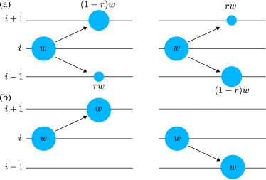
The stochastic process for the evolution of trails takes place in one spatial dimension. In our model, both space and time are discrete. At each timestep, every trail may split, with probability $p$, into two smaller trails, or remain intact with the complementary probability $1-p$ (see figure 1). In the former case, two trails are created with weights that are fractions $r$ and $1-r$ of the weight of the parent trail, and hence, the overall weight is conserved. Trails also move randomly, and essentially perform a simple random walk. Finally, when two trails collide, they merge, with the overall weight being a conserved quantity.

Regardless of the initial conditions, the system evolves toward a steady state. We study the steady-state density $P(w)$ of trails with weight $w$ and find the power-law behavior

$$P(w)\sim w^{-\gamma},$$ (1)

for small weights, $w\to 0$. Interestingly, the power-law exponent varies continuously with the fragmentation probability $p$ and the fragmentation ratio $r$ as $\gamma$ is a real root of the equation

$$r^{\gamma-1}+(1-r)^{\gamma-1}=\frac{3-p}{1-p}\,.$$ (2)

Results of our numerical simulations are in excellent agreement with this theoretical prediction. Depending on the parameters $p$ and $r$, the exponent $\gamma<1$ can be positive such that small-weight trails are enhanced, or it can be negative such that small-weight trails are suppressed. Our theoretical approach assumes that spatial correlations are absent at the steady state, and our extensive numerical simulations support this assumption.

The rest of this manuscript is organized as follows. Section II introduces the model, and section III provides an elementary derivation of the trail concentration. In section IV, we analyze the density of trail weights theoretically and numerically. We obtain analytic expressions for moments of the trail density, and also, obtain the distribution of small weights. Section V addresses the weak fragmentation limit where aggregation and fragmentation proceed independently. In this limit, dynamical properties of voids between adjacent trails can be understood using first-passage properties of an ordinary random walk. We discuss applications of the model to physical problems, in particular to trajectories of particles in complex flows in section VI, and conclude in section VII.

II The model

Our aggregation-fragmentation-diffusion model takes place on an unbounded lattice in one dimension. A lattice site labeled $i$ may be either vacant or occupied by a trail with weight $w_{i}$. The weight can also be understood as density of a trail of particles concentrated at location $i$. In the initial configuration, each site is occupied by a trail with weight unity.

The stochastic process has three elements: (i) Fragmentation. With the probability $p$, a trail with weight $w_{i}$ splits into two fragments with weights $rw_{i}$ and $(1-r)w_{i}$. One of these fragments moves to neighboring site $i-1$ and the remaining fragment moves to neighboring site $i+1$. The two realizations are equally likely (see figure 1). (ii) Diffusion: With the complementary probability $1-p$ the trail remains intact and it moves, with equal probabilities, to site $i-1$ or to site $i+1$. (iii) Aggregation. All sites are updated simultaneously according to the fragmentation and diffusion steps above. When two distinct trails arrive at the same site, they immediately merge to form a new trail whose weight equals the sum of those of the two original trails.

Figure 2: A numerical realization of the aggregation-fragmentation-diffusion process with $r=0.01$ and $p=0.05$. The color coding illustrates weights from low (blue) to high (yellow) values, and the color bar is in natural logarithmic scale. Unoccupied sites are dark purple.

Hence, two parameters characterize the model: the fragmentation probability, $p$ with $0<p<1$, and the fragmentation ratio, $r$ with $0<r<1$. These parameters control how the weight at each site evolves prior to the final aggregation step,

$$w\to\begin{cases}rw,(1-r)w&\quad{\rm with\ prob.\ }p\,,\\ w&\quad{\rm with\ prob.\ }1-p\,.\end{cases}$$ (3)

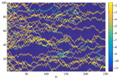
All trails are updated simultaneously, and time $n$ is augmented by one after each iteration, $n\to n+1$. Essentially, trails perform a random walk (see figure 2), and importantly, mobility is not coupled to weight. We stress that total trail weight is conserved since both fragmentation and aggregation are conservative processes.

Our Monte Carlo simulations were performed using a regular lattice with $N$ sites and periodic boundary conditions. Initially, each site is occupied with a trail of unit weight. In each iteration, all sites are updated simultaneously according to the model rules. Namely, a trail jumps without splitting to a neighboring site with probability $1-p$, or decomposes into two fragments, with probability $p$, as in figure 1 and equation (3). Two trails landing at iteration $n$ at the same location immediately merge. Figure 2 shows trajectories in a space-time diagram using simulation data.

III The concentration

We first study the trail concentration $c$, defined as fraction of occupied sites. Our primary focus is the steady state, where the competing processes of aggregation and fragmentation balance each other. The fragmentation ratio $r$ affects the trail weight but it does not affect the number of trails. Hence, the concentration depends on the fragmentation probability $p$ alone. By assuming that occupations at neighboring sites are not correlated, we can write a closed equation for the concentration. In each fragmentation event a single trail generates two trails and conversely, in each aggregation event two trails coalesce into one. At the steady state, the gain rate and the loss rate balance,

$$p\,c=\left(\frac{1+p}{2}c\right)^{2}\,.$$ (4)

The fragmentation rate on the left-hand-side is proportional to the concentration $c$ and the fragmentation probability $p$. The aggregation rate equals the probability that two trails arrive at the same site. The quantity in parentheses is the sum of $p\,c$ and $\frac{1-p}{2}c$ accounting for trail fragments and intact trails respectively (see figure 1). In writing the quadratic aggregation term in (4), we make the assumption that the occupancy at a site is not correlated with that at its next-nearest neighbor.

Figure 3: Numerically computed trail concentration $c(p)$ versus the fragmentation probability $p$. The dashed line corresponds to the analytic expression (5), and circles to Monte Carlo simulations on a lattice of $N=10^{6}$ sites.

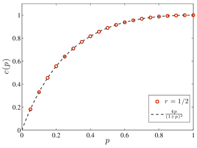
Rearranging Eq. (4) we find the trail concentration

$$c=\frac{4p}{(1+p)^{2}}\,.$$ (5)

Figure 3 shows a comparison of Eq. (5) with numerical simulations of the model. The numerical results indicate that spatial correlations in the trail concentration disappear in the steady state. Qualitatively, the equilibrium concentration of domain walls in the one-dimensional Ising model with single-spin flip dynamics exhibits similar phenomenology rjg ; zr ; gns .

The trail concentration has the following limiting behaviors

$$c\simeq\begin{cases}4p&\quad p\to 0\,,\\ 1-\frac{1}{4}(1-p)^{2}&\quad p\to 1\,.\end{cases}$$ (6)

The concentration vanishes linearly when $p\to 0$, and hence, the average trail weight which according to mass conservation is inversely proportional to $c$, diverges in this limit. Also, the fraction of vacant sites vanishes quadratically when $p\to 1$.

IV The weight density

We now turn to the main focus of our investigation, the steady-state weight density. Our theory builds on the results of section III, and using the assumption that weights at different sites are not correlated, we can accurately predict key statistical properties of the weight density.

We define the weight density $P(w)$ such that $P(w)dw$ is the fraction of sites occupied by a trail with weight in the infinitesimal range $[w:w+dw]$. Trail weight is conserved throughout the aggregation-fragmentation-diffusion process and hence, the total weight density $\int dw\,w\,P(w)$ is a constant. The concentration $c$ equals the integrated weight density

$$c=\int_{0}^{\infty}dw\,P(w)\,.$$ (7)

The normalized quantity $c^{-1}P(w)$ is the probability distribution function for the weight.

Changes in trail weight occur in two stages: first, before trails move and then, after they move. In the first stage, trail weight may change by fragmentation. Let $G(w)$ be the weight density of trails produced at the first stage. According to the random process (3), we have

$$G(w)=\frac{p}{r}P\left(\frac{w}{r}\right)+\frac{p}{1-r}P\left(\frac{w}{1-r}\right)+(1-p)P(w)\,.$$ (8)

Here, the first two terms on the right-hand side account for fragments and the last term accounts for intact trails. As also follows from Eq. (8), weight conservation sets $\int dw\,w\,G(w)=\int dw\,w\,P(w)$, and the fragmentation rule (3) implies $\int dw\,G(w)=(1+p)\int dw\,P(w)$.

In the steady state, the trail density before an iteration, $P(w)$, is unchanged after one iteration of the combined aggregation-fragmentation diffusion process. This is expressed by the nonlinear-integral equation:

$$P(w)=\left(\!1-\frac{1+p}{2}c\!\right)\!G(w)+\frac{1}{4}\int_{0}^{w}\!\!dv\,G(v)G(w-v).$$ (9)

The first term on the right-hand side accounts for the scenario where there is no aggregation. It is a product of three factors: (i) The quantity $G(w)/2$ which represents a trail produced at a neighboring site and where the factor $1/2$ accounts for the equal distribution of weight from one site to its two neighbors, (ii) The factor $2$ accounting for two neighbors, and (iii) The probability $1-\tfrac{1+p}{2}c$ that such a trail avoids aggregation. This probability sums $1-c$ and $\tfrac{1-p}{2}c$ for a vacant and an occupied next-nearest neighbor, respectively. The second term on the right-hand side is the aggregation term; it is a convolution of two identical terms of the form $G(w)/2$ with $G(w)$ given by (8). By integrating Eq. (9) over all weights, we recover equation (4), and furthermore, this equation is consistent with mass conservation.

We stress that substitution of equation (8) into (9) turns the latter into a closed, nonlinear, equation for the weight density $P(w)$. Compared with Eq. (4), the steady-state equation (8) makes an even stronger assumption that weights at different sites are not correlated. Indeed, the convolution term in (9) which accounts for the weight of aggregates is quadratic in the density $P(w)$.

IV.1 Moment Analysis

To examine the validity of this no-correlation assumption, we study the moments of the weight density,

$$M_{k}=\int dw\,w^{k}P(w)\,.$$ (10)

Of course, the zeroth moment corresponds to the total concentration $M_{0}=c$, and the first moment $M_{1}=1$ corresponds to the total weight density which is a conserved quantity. As shown in Fig. 3, the numerical simulations confirm the predictions of (9) for the zeroth moment.

Figure 4: The normalized second and third moments $m_{2}(n)=M_{2}(n)/2$ and $m_{3}(n)=M_{3}(n)/6$, versus: (a) $n$, and (b) $n^{-1/2}$. Shown are results of Monte Carlo simulations on a ring with $10^{8}$ sites for the case $r=p=1/2$. A fourth order polynomial fit to $m_{k}(n)$ versus $n^{-1/2}$ yields the asymptotic values $1.0001$ and $1.0002$ for $m_{2}(\infty)$ and $m_{3}(\infty)$.

We now introduce the Laplace transform $M(s)=\int_{0}^{\infty}dwe^{-sw}P(w)$ which is the generating function of the moments,

$$M(s)=\sum_{n=0}^{\infty}\frac{(-s)^{k}}{k!}M_{k}\,.$$ (11)

By first substituting the concentration (5) into (9), then multiplying equation (9) with $e^{-sw}$, and finally, integrating over weight, we find that the Laplace transform obeys the nonlinear equation

$$M(s)=\frac{1-p}{1+p}\,U(s)+\frac{1}{4}U^{2}(s)\,,$$ (12)

with $U(s)=pM(rs)+pM(s-rs)+(1-p)M(s)$. The quantity $U(s)$ is the following Laplace transform $U(s)=\int dwe^{-sw}G(w)$, and it can be conveniently expressed in terms of the moments $M_{k}$,

$$U(s)=\sum_{n=0}^{\infty}\frac{(-s)^{k}}{k!}\,u_{k}\,M_{k}\,.$$ (13)

Here, $u_{k}=1-p[1-r^{k}-(1-r)^{k}]$, and we quote the values $u_{0}=1+p$, $u_{1}=1$, and $u_{2}=1-2pr(1-r)$. Using $M(0)=c$ and $U(0)=(1+p)c$, we can recover from (12) the trail concentration (5). Mass conservation dictates that $M_{1}$ equals the initial mass density. In general, the moments satisfy the recursion

$$M_{k}=\frac{1}{4(1-u_{k})}\sum_{l=1}^{k-1}\binom{k}{l}u_{l}u_{k-l}M_{l}M_{k-l}\,,$$ (14)

when $k\geq 2$. In particular, the second and third moments are given by

$$M_{2}=\frac{M_{1}^{2}}{2(1-u_{2})}\,,\quad M_{3}=\frac{3\,u_{2}\,M_{1}^{3}}{4(1-u_{2})(1-u_{3})}\,.$$ (15)

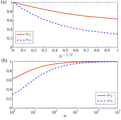
For the special case $p=r=1/2$ with $M_{1}=1$, we have $M_{0}=8/9$, $M_{2}=2$ and $M_{3}=6$. Results of our Monte Carlo simulations are in excellent agreement with these theoretical predictions (see figure 4). We also verified numerically that (15) holds for other values of the fragmentation probability $p$ and the fragmentation ratio $r$, and for a variety of initial conditions.

Figure 5: The power-law tail of the weight density $P(w)$. The curves shown here correspond to different values of $p$, indicated in the legend, and are obtained from Monte Carlo simulations on a lattice of $N=10^{6}$ sites. Dashed lines correspond to the theoretical predictions of equations (1)-(2). The value of $r$ was chosen to be $r=0.01$. The inset displays the case $r=0.25$ and $p=0.7$ for which $\gamma=-0.32$.

We have also examined numerically the empty-interval probability $E_{l}$ that $l$ consecutive sites are vacant. As expected given the absence of spatial correlations, we confirmed the exponential behavior $E_{l}=E_{1}^{l}$ with $E_{1}=1-c$ and $c$ given in (5). Our preliminary analytic results for the simpler case of sequential dynamics where sites are updated one at a time show that spatial correlations do not vanish, and therefore, qualitative features of the steady state are sensitive to details of the dynamics.

Below, we discuss the small-weight statistics of the trail density and provide numerical results that confirm the theoretical predictions. Based on the simulation results, we conclude that at the steady state, spatial correlations in trail weight disappear. A similar behavior occurs in adsorption-desorption processes pb ; kb ; jtt where gaps between adsorbed particles in one-dimension essentially undergo an aggregation-fragmentation process, and also, in a related model for the propagation of force chains in granular matter cmnw .

Figure 6: (a) The exponent $\gamma$ for different values of $p$ and $r$. The lines correspond to the theoretical predictions, given by Eq. (2), for different values of $r$, see the legend. The inset shows the region of negative $\gamma$ as shaded. (b) When data is plotted as $r^{\gamma-1}+(1-r)^{\gamma-1}$ it collapses into the curve $(3-p)/(1-p)$ (solid line) in accord with (2).

The results of section III imply that in a finite system, every configuration with $N_{1}$ occupied sites and $N_{2}$ vacant sites is realized with the equilibrium probability $c^{N_{1}}(1-c)^{N_{2}}$ that corresponds to a noninteracting two-state system. The moment analysis indicates that an even stronger statement applies as all states with the same configuration of weights are equally probable. In essence, the weight density $P(w)$ completely describes the system.

IV.2 Small-weight statistics

We now focus on the small-weight tail of the density $P(w)$. In the limit $w\to 0$, the nonlinear terms become negligible. If we substitute the concentration given in (5) into (9), we find that the small-$w$ tail of the steady-state density $P(w)$ satisfies the linear equation

$$\frac{1}{r}P\left(\frac{w}{r}\right)+\frac{1}{1-r}P\left(\frac{w}{1-r}\right)=\frac{3-p}{1-p}P(w)\,.$$ (16)

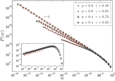
From this equation we arrive at our main result, the power-law behavior $P(w)\sim w^{-\gamma}$ with the exponent $\gamma$ being root of Eq. (2). Clearly, the exponent $\gamma<1$ varies continuously with the model parameters $r$ and $p$. In the special case $r=1/2$ we have $\gamma=2-(\ln\tfrac{3-p}{1-p})/\ln 2$.

Figure 7: The exponent $\gamma$ versus the parameter $r$ for small values of $p$.

The small-weight statistics also follow from the Laplace transform. When $M(s)$ is small, the nonlinear term in the governing equation (12) is negligible, thereby leading to the linear equation $(1+p)M(s)=(1-p)U(s)$. This equation implies the large-$s$ decay $M(s)\sim s^{\gamma-1}$, which is equivalent to the power-law behavior (1), with the exponent $\gamma$ root of equation (2).

Figure 8: (a) Voids are defined as closed regions of unoccupied sites and they are defined by an area $S$ (blue region) and duration $T$. (b) and (c) PDF of the void durations and sizes, respectively, for two different values of $p$ and $r=0.01$. Solid red lines correspond to a power law with exponent $-3/2$ (b) and $-4/3$ (c).

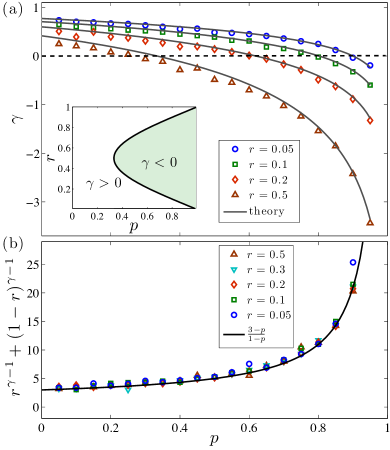
Our numerical simulations provide excellent support for equation (2). Figure 5 demonstrates the power-law tail of the weight density, and figure 6 compares the numerically-computed exponent $\gamma$ for different model parameters with the theoretical prediction.

In a finite system of size $N$, the power-law tail (1) holds in the range $N^{-1/(1-\gamma)}\ll w\ll 1$. The lower limit follows from the criterion $N\int_{0}^{z}dw\,P(w)\sim 1$ which gives an estimate for the scale $z$ of the smallest weight in the system krb . The scaling law $z\sim N^{-1/(1-\gamma)}$ explains the large variation in the extent of the power-law regime observed in figure 5.

Equation (2) implies that there are two distinct regimes of behavior, since the exponent $\gamma$ vanishes when

$$r(1-r)=\frac{1-p}{3-p}\,.$$ (17)

As shown in figure 6a, $\gamma$ can be positive, in which case, the density of small-weight tails is enhanced. In the complementary regime, $\gamma$ is negative and small-weight trails are suppressed. When $p<1/3$ the exponent is always positive, $\gamma>0$.

The linear equation (16) reflects the nature of the fragmentation process in which weight “cascades” from small trails into even smaller trails according to $w\to rw,(1-r)w$ . This cascade process is balanced by aggregation of small trails into larger trails. The power-law behavior is valid over a substantial size range, and throughout this range only terms that are linear in $P(w)$ dominate Eq. (9). Qualitatively similar cascades, where the full nonlinear theory reduces to a linear theory for extreme-value statistics, are found in wave turbulence crz ; zlf and inelastic gases bm . Yet, the cascade process described by equation (16) has two distinctive features. First, the tail (1) can be vanishing or diverging. Second, in equation (9), the term linear in $P(w)$ is also proportional to the trail concentration $c$. Consequently, the prefactor on the right-hand side of (16) depends on the steady-state value (5) of the concentration, and despite its linear nature, this equation does incorporate a two-point correlation.

For completeness, we mention that we also numerically studied the large-$w$ tail of the weight density. In contrast with the broad power-law tail that may occur at small weights, we find that large weights are exponentially rare, $P(w)\sim\exp(-{\rm const.}\times w)$ for $w\gg 1$. This behavior is consistent with the large-size statistics found in irreversible aggregation fl and in the closely related $q$-model for force chains lnscmnw ; cmnw .

IV.3 Stochastic Fragmentation

The fragmentation process in (3) is deterministic in the sense that the sizes of the two trail fragments are fixed fractions of the original trail. We briefly mention a natural counterpart, stochastic fragmentation, where the fraction $0<r<1$ is drawn from the distribution $\eta(r)$. We require that the distribution be: (i) normalized $\int_{0}^{1}dr\eta(r)=1$, and (ii) symmetric $\eta(r)=\eta(1-r)$. It is straightforward to generalize the above theoretical analysis to stochastic fragmentation and in particular, equation (2) becomes

$$\int_{0}^{1}d\eta\,\eta(r)\left[r^{\gamma-1}+(1-r)^{\gamma-1}\right]=\frac{3-p}{1-p}\,.$$ (18)

For the so-called random-scission model krb ; cmnw where the fraction $r$ is uniformly distributed, $\eta(r)=1$, we find

$$\gamma=2\,\frac{1-p}{3-p}\,.$$ (19)

In this case, the exponent $\gamma$ satisfies $0<\gamma<2/3$, and the small-weight tail of the distribution is enhanced, regardless of $p$.

V Weak Fragmentation

We now analyze the small $p$ case and show that aggregation and fragmentation proceed independently in this regime. In the limit $p\to 0$, the trail concentration vanishes, see Eq. (5), and consequently, $P(w)\propto p$. By keeping dominant terms of the order ${\cal O}(p^{2})$ and neglecting sub-dominant terms of the orders ${\cal O}(p^{3})$ and ${\cal O}(p^{4})$, we find that equation (9) simplifies to

$$0 = 4p\left[\frac{1}{r}P\left(\frac{w}{r}\right)+\frac{1}{1-r}P\left(\frac{w}{1-r}\right)-P(w)\right]$$ (20)

$$+ \int_{0}^{w}{\rm d}y\ P(y)P(w-y)-2\,c\,P(w)\,.$$

The first two (linear) terms account for fragmentation, while the next two (nonlinear) terms account for aggregation between two intact trails. Thus, fragmentation and aggregation are not coupled when fragmentation is weak. As a check of self-consistency, we integrate (20) to find $c^{2}=4p\,c$. Hence, the concentration is proportional to the fragmentation probability $c\simeq 4p$ as in (6).

In the limit $w\to 0$, the nonlinear term in Eq. (20) is negligible, and the linear terms satisfy

$$\frac{1}{r}P\left(\frac{w}{r}\right)+\frac{1}{1-r}P\left(\frac{w}{1-r}\right)=3P(w)\,.$$ (21)

This linear equation accepts a solution of algebraic form $P(w)\sim w^{-\gamma}$ for small $w$, where the exponent $\gamma<1$ is root of the equation

$$r^{\gamma-1}+(1-r)^{\gamma-1}=3.$$ (22)

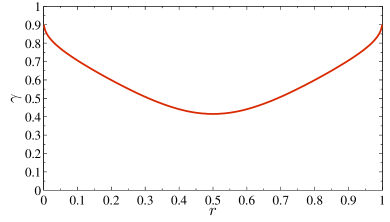
Figure 7 shows a plot of $\gamma(r)$ as given by the above equation where we observe that the minimal value $\gamma=2-\frac{\ln 3}{\ln 2}$ is attained when $r=1/2$.

As discussed above, when fragmentation is weak, the trail concentration is low. Moreover, since fragmentation events are rare, fragmentation and aggregation proceed independently. In this limit, it is relatively simple to characterize the dynamics of voids between adjacent trails. In the limit $p\to 0$, trails merely perform a random walk, and when two trails come to within distance of two sites, there is a finite probability for the two to coalesce. Hence, the problem is equivalent to a first-passage process of a simple random walk (the distance between two independent random walks itself performs a random walk). Let $T$ be the lifetime of a void between two trails and $Q(T)$ be the probability a void has a lifetime $T$ (see figure 8a). Using the well-known return probability of a random walk sr , we conclude (see figure 8b)

$$Q(T)\sim T^{-3/2}\,.$$ (23)

Furthermore, we can also consider the area $S$ of a void in a space-time diagram (see figure 8a). Because the edges of the void are random walks, the width of the void scales as $T^{1/2}$ and consequently the area scales as $S\sim T^{3/2}$. Using $R(S)$ for the probability of observing a void with area $S$, the scaling behavior (see figure 8c)

$$R(S)\sim S^{-4/3}\,,$$ (24)

follows immediately from (23). Our numerical simulation results, shown in figures 8b and 8c, support the first-passage behaviors (23) and (24).

VI Applications

The aggregation-fragmentation-diffusion process can be used to model the migration trails of animals bm1 ; ra . In this application the time variable is viewed as a second space coordinate, along which the animal migration is directed, for example north to south. Movement along the transverse direction is random. The migrating animals are assumed to choose the easiest path with a component in their intended direction of travel. In a random landscape, the trails will fluctuate in direction, and different trails may combine. Fragmentation would occur if there is some inhomogeneity in the population, so that there may be a difference in which is the easiest path for different individuals. For example, in human migration, people traveling on foot may be able to follow a trail which would not be accessible in a wheeled vehicle.

Another motivation for our study comes from a theoretical model of particles in a compressible turbulent flow in one dimension of space rg ; mr ; fgv ; tb ; gm ; pw . Specifically, consider a large number of trajectories, in a system with periodic boundary conditions, evolving according the dynamical system defined in pphw ; hppw . Assuming that the trajectories are initially uniformly distributed in space, trajectories tend to aggregate and form strongly concentrated clusters, leading to an extremely heterogeneous distribution of “mass” in space and time. The merging and splitting particle trajectories pphw ; hppw share many qualitative similarities with those shown in Figure 2.

The analogy is in fact more than qualitative. The existence of large regions, with an extremely small concentration of particles is characterized in the particle problem, and in the aggregation-fragmentation-diffusion model in the weak $p$ limit, by a power-law behavior of the area $S$ of the empty regions in a space-time diagram, defined in Fig. 8a, with an exponent $4/3$ pphw . This points to similar mechanisms to explain the large heterogeneities in both models. Furthermore, dividing space into small bins, and defining the weight $w$ as the number of trajectories per bin at a given instant of time, one finds a power-law distribution of $w$ as in Eq. (1) pphw . Over the range of control parameters in the model, the exponent $\gamma$ is always positive, implying a very large probability of empty regions. It would be interesting to explore further analogies between the present model of aggregation-fragmentation-diffusion, and the theoretical model for particle transport by compressible turbulent flows. The resulting theoretical understanding should provide insight on experimental observations on the dispersion of particles on a surface flow lbgp .

VII Discussion

We have studied an aggregation-fragmentation-diffusion random process that describes the evolution of trails of particles with local weight density. In our model, a trail may fragment into two or it may stay intact. In addition, trails move randomly, essentially performing diffusion. Aggregation occurs when two trails arrive at the same location. The model is characterized by two parameters, the fragmentation probability which controls the relative strength of the fragmentation process, and the fragmentation ratio which controls the size of the produced fragments. An equilibrium state is found, where the two competing processes of aggregation and fragmentation balance each other. In this steady state, the small-weight tail of the fragment density has a power-law tail. The exponent governing this tail varies continuously with the model parameters.

At the core of our theoretical approach are the assumptions that the occupancy and even the weights of trails at different locations are uncorrelated. Our extensive numerical simulations confirm this behavior. The system achieves an equilibrium state, where aggregation and fragmentation are in perfect balance, with the remarkable property that all configurations with the same number of trails are equally probable. Usually, it is possible to trace such behavior to a detailed balance condition where there is zero net flux between any two microscopic configurations of the system. It is an interesting challenge to construct an equivalent condition for our synchronous dynamics.

Interestingly, our numerical results also show that spatial correlations do exist at all times and only at the steady state do they strictly vanish. It is straightforward to convert the steady-state equation (9) into a discrete-time recursion equation for the weight density. Such recursion equation implies fast exponential relaxation toward the steady state, $dM_{k}/dn\sim\exp[-(1-u_{k})n]$ for $k\geq 2$. However, our simulations reveal slow algebraic relaxation instead (figure 4) $dM_{k}/dn\sim n^{-3/2}$, for $k\geq 2$. Spatial correlations, which steadily diminish with time and eventually disappear altogether, are responsible for slow relaxation toward the steady state. The diffusive relaxation we observe numerically is consistent with the first-passage behavior (23), and is reminiscent of time-dependent behavior in reaction-diffusion processes involving aggregation in one spatial dimension jls ; brt ; bdb .

The authors are grateful to the Kavli Institute for Theoretical Physics for support, where this research was supported in part by the National Science Foundation under Grant No. PHY11-25915.

References

- (1) P. L. Krapivsky, S. Redner and E. Ben-Naim, A Kinetic View of Statistical Physics (Cambridge University Press, Cambridge, 2010).
- (2) R. D. Vigil, R. M. Ziff, and B. Lu, Phys. Rev. B 38, 942 (1988).
- (3) P. L. Krapivsky and S. Redner, Phys. Rev. E 54, 3553 (1996).
- (4) S. N. Majumdar, S. Krishnamurthy, and M. Barma, Phys. Rev. Lett. 81, 3691 (1998).
- (5) E. Ben-Naim and P.L. Krapivsky Phys. Rev. E 77, 061132 (2008).
- (6) D. A. Lowe and L. Thorlacius, Phys. Rev. D 51, 665 (1995).
- (7) P. J. Blatz and A. V. Tobolsky, J. Phys. Chem. 49, 77 (1945).
- (8) R. Rajesh and S. N. Majumdar, Phys. Rev. E 63, 036114 (2001).
- (9) R.D. Vigil, J. Coll. Int. Sci. 336, 642 (2009).
- (10) A. E. Scheidegger, Water Resources Research 3, 103 (1967).
- (11) G. Huber, Physica A 170, 463 (1991).
- (12) C.H. Liu, S.R.Nagel, D.A. Schecter, S.N. Coppersmith, S. Majumdar, O. Narayan, T.A. Witten, Science 269, 513 (1995).
- (13) S.N. Coppersmith, D. Majumdar, O. Narayan, and T.A. Witten, Phys. Rev. E 53, 4673 (1996).
- (14) P. J. Flory, J. Amer. Chem. Soc. 63, 3083 (1941).
- (15) A. A. Lushnikov, J. Colloid. Inter. Sci. 65, 276 (1977).
- (16) R. M. Ziff, E. M. Hendriks, and M. H. Ernst, Phys. Rev. Lett. 49, 593 (1982).
- (17) P. G. J. van Dongen and M. H. Ernst, J. Stat. Phys. 49, 879 (1987).
- (18) F. Leyvraz, Phys. Rep. 383, 95 (2003).
- (19) A. F. Filippov, Theory Prob. Appl. 6, 275 (1961).
- (20) E. D. McGrady and R. M. Ziff, Phys. Rev. Lett. 58, 892 (1987).
- (21) Z. Cheng and S. Redner, J. Phys. A 23, 1233 (1990).
- (22) M. H. Ernst and G. Szamel, J. Phys. A 26, 6085 (1993).
- (23) P.L. Krapivsky and E. Ben-Naim Phys. Rev. E 68, 021102 (2003).
- (24) M. Pradas, A. Pumir, G. Huber, and M. Wilkinson, arXiv: 1701.08262.
- (25) G. Huber, M. Pradas, A. Pumir, and M. Wilkinson, (submitted).
- (26) R. J. Glauber, J. Math. Phys. 4, 294 (1963).
- (27) Z. Rácz, Phys. Rev. Lett. 55, 1707 (1985).
- (28) M. D. Grynberg, T. J. Newman, R. B. Stinchcombe, Phys. Rev. E 50, 957 (1994).
- (29) V. Privman and M. Barma, J. Chem. Phys. 97, 6714 (1992).
- (30) P. L. Krapivsky and E. Ben-Naim, J. Chem. Phys. 100, 6778 (1994).
- (31) X. Jin, G. Tarjus, and J. Talbot, J. Phys. A 27, L195 (1994).
- (32) C. Connaughton, R. Rajesh, and O. Zaboronski, Phys. Rev. Lett. 98, 080601 (2007).
- (33) V. E. Zakharov, V. S. Lvov, and G. Falkovich, Kolomogorov Spectra of Turbulence I: Wave Turbulence (Springer-Verlag, New York, 1992).
- (34) E. Ben-Naim and J. Machta, Phys. Rev. Lett. 94, 138001 (2005).
- (35) S. Redner, A Guide to First-Passage Processes Cambridge, University Press, (2001).
- (36) L. P. Brower and S. B. Malcolm, American Zooogist 31, 265 (1991).
- (37) R. M. Alexander, Journal of Avian Biology 29, 387 (1998).
- (38) R. Gatignol, J. Méc. Théor. Appl. 1, 143 (1983).
- (39) M. R. Maxey and J. J. Riley, Phys. Fluids 26, 883 (1983).
- (40) G. Falkovich, K. Gawedzki, and M. Vergassola, Rev. Mod. Phys. 73, 913 (2001).
- (41) F. Toschi and E. Bodenschatz, Annu. Rev. Fluid Mech. 41, 375 (2009).
- (42) K. Gustavsson and B. Mehlig,, Adv. in Phys. 65, 1 (2016).
- (43) A. Pumir and M. Wilkinson, Ann. Rev. Cond. Matter Phys. 7, 141 (2016).
- (44) J. Larkin, M. M. Bandi, A. Pumir, and W. I. Goldburg, Phys. Rev. E 80, 066301 (2009).
- (45) J. L. Spouge, Phys. Rev. Lett. 60, 871 (1988).
- (46) B. R. Thomson, J. Phys. A 22, 879 (1989)
- (47) M. A. Burschka, C. R. Doering, D. Ben avraham, Phys. Rev. Lett. 63, 700 (1989).