A return to eddy viscosity model for epistemic UQ in RANS closures

1 Motivation and objectives

Due to their computational tractability, closure models based on the Reynolds-Averaged Navier-Stokes (RANS) equations remain a widely used option for the computation of turbulent flow fields. However, the numerous assumptions made in their derivation and calibration result in models subject to unknown degrees of parametric and epistemic model-form uncertainty. This in turn leads to flow-dependent performance and ultimately to predictions which can be trustworthy for certain regions of a flow domain, yet highly erroneous in others.

Various attempts have been made to quantify the uncertainty in RANS closures. Bayesian inference can be used to obtain stochastic estimates of the closure coefficients, (see, e.g., (Edeling et al., 2014)). A limitation is that just varying the coefficients does not challenge the underlying Boussinesq hypothesis. Also, the obtained posterior distributions on the coefficients have no direct spatial dependence. They are applied uniformly throughout the flow domain, regardless of the degree of local model failure.

Recently, Machine-Learning (ML) algorithms have also found application to the problem. For instance (Zhang & Duraisamy, 2015) have applied neural nets and Gaussian processes to directly infer new so-called adjustment terms from high-fidelity data. These terms are added to an existing closure model with the intention of correcting for the RANS bias. As they are trained on local input features, the adjustment term is able to vary spatially.

Although promising results have been obtained, (see, e.g., (Wu et al., 2016)), ML techniques are not without their drawbacks. Depending on the chosen ML algorithm, the inverse problem can be high-dimensional. Also, taking a neural network as an example, the manner in which it arrives at the complex input-output relation is not easy to interpret in physical terms and therefore does not necessary lead to increased confidence. Furthermore, the process is entirely dependent on the training and calibration data used and therefore possibly is of limited universality. And although it can approximate complex functions, it yields no analytical form to study the structure of the model discrepancy.

We will build upon the work of (Emory et al., 2013), in which perturbations in the eigenvalues of the anisotropy tensor are introduced in order to bound a Quantity-of-Interest (QoI) based on limiting states of turbulence. To make the perturbations representative of local flow features, we introduce two additional transport equations for linear combinations of these aforementioned eigenvalues. The model form is inspired by the LAG model of (Olsen & Coakley, 2001), which perturbs the eddy-viscosity at locations where a failure of the Boussinesq hypothesis might reasonably be anticipated. The location, magnitude and direction of the eigenvalue perturbations are now governed by the model transport equations. The general behavior of our discrepancy model is determined by two coefficients, resulting in a low-dimensional Uncertainty Quantification (UQ) problem. We will furthermore show that the behavior of the model is intuitive and rooted in the physical interpretation of misalignment between the mean strain and Reynolds stresses.

In this paper we will focus on estimating prediction intervals on QoIs. Obtaining data-driven distributions within those intervals in a Bayesian setting is the subject of ongoing research. In this sense, the intervals of this paper might be considered as the results of propagating uniform prior distributions on the two coefficients.

The structure of the paper is as follows. In Section 2 we discuss the representation of the Reynolds stress anisotropy, followed by a section on the model transport equations and their properties. Section 4 covers the obtained intervals on the QoI and finally, we close by presenting our conclusions in Section 5.

2 Reynolds stress anisotropy and the barycentric map

A RANS closure employed by many turbulence models is the Boussinesq hypothesis, which reads

$$\overline{u^{\prime}_{i}u^{\prime}_{j}}\approx\frac{2}{3}k\delta_{ij}-2\nu_{T}S_{ij}.$$ (1)

Here, $k$ is the turbulent kinetic energy, $\delta_{ij}$ the Kronecker delta, and $S_{ij}$ is the mean strain rate tensor, defined as $S_{ij}:=\frac{1}{2}\left({\partial\overline{u}_{i}}/{\partial x_{j}}+{\partial\overline{u}_{j}}/{\partial x_{i}}\right)$ in the case of incompressible flow. The scalar quantity $\nu_{T}$ is the eddy-viscosity, which must be computed by means of a chosen turbulence model, e.g. the $k-\varepsilon$, $k-\omega$ or Spalart-Allmaras model (Wilcox, 1998). Although we will use the $k-\varepsilon$ model, all closure models have their own specific mathematical form, closure coefficients and corresponding uncertainties, ultimately leading to an uncertain $\nu_{T}$ (Edeling et al., 2014). Instead of focusing on $\nu_{T}$, we will inject uncertainty directly into $\overline{u^{\prime}_{i}u^{\prime}_{j}}$ by adding a tensorial discrepancy model $E_{ij}$ to the right-hand side of Eq. (1), leaving any underlying baseline turbulence model unperturbed. To this end, let us define the normalized anisotropy tensor $b_{ij}$ as

$$b_{ij}:=\frac{\overline{u^{\prime}_{i}u^{\prime}_{j}}}{2k}-\frac{1}{3}\delta_{ij};\quad-\frac{1}{3}\leq b_{\alpha\alpha}\leq\frac{2}{3};\quad-\frac{1}{2}\leq b_{\alpha\beta}\leq\frac{1}{2};$$ (2)

which is a symmetric, deviatoric (zero trace) tensor. Greek subscripts are excluded from the summation convention. Tensor invariants of $b_{ij}$ are a useful tool to study the anisotropy. These invariants are defined as

$$\mathrm{I}_{b}=b_{ii}\quad\mathrm{II}_{b}=b^{2}_{ii}=b_{ij}b_{ji}\quad\mathrm{III}_{b}=b^{3}_{ii}=b_{ij}b_{jk}b_{ki}.$$ (3)

Since $b_{ij}$ is deviatoric ($\mathrm{I}_{b}=0$), only two invariants are needed to characterize the state of anisotropy. The invariants in Eq. (3) are non-linear functions of the eigenvalues of $b_{ij}$, (see, e.g., (Lumley & Newman, 1977)). More recently, other invariant measures have been proposed by (Banerjee et al., 2007) which have a linear relationship with the eigenvalues of $b_{ij}$. As our framework will involve inverting the relation between the invariants and the eigenvalues, these linear measures are preferred.

Banerjee expresses the anisotropy tensor as a convex combination of three basis tensors $\hat{b}_{1c}$, $\hat{b}_{2c}$, $\hat{b}_{3c}$, i.e.,

$$\hat{b}_{ij}=C_{1c}\hat{b}_{1c}+C_{2c}\hat{b}_{2c}+C_{3c}\hat{b}_{3c}.$$ (4)

These basis tensors represent the three limiting states of componentality (relative strengths of components in $\overline{u^{\prime}_{i}u^{\prime}_{j}}$), i.e., they represent one-, two- and three-component turbulence. The modified notation $\hat{b}_{ij}$ represents the anisotropy tensor in principal axes,

$$\hat{b}_{ij}=\mathrm{diag}\left(\lambda_{1},\lambda_{2},\lambda_{3}\right),$$ (5)

where $\lambda_{1}\geq\lambda_{2}\geq\lambda_{3}$. The basis tensors are defined as

$$\hat{b}_{1c}=\mathrm{diag}\left(2/3,-1/3,-1/3\right),\;\;\hat{b}_{2c}=\mathrm{diag}\left(1/6,1/6,-1/3\right),\;\;\hat{b}_{3c}=\mathrm{diag}\left(0,0,0\right),$$ (6)

where $\hat{b}_{3c}$ corresponds to the isotropic limit.

From Eq. (4) it is clear that the coefficients $C_{1c}$, $C_{2c}$ and $C_{3c}$ measure how close $\hat{b}_{ij}$ is to any of the three limiting states. Since Eq. (4) is required to be a convex combination, we have by definition:

$$C_{1c}+C_{2c}+C_{3c}=1\;\;\mathrm{and}\;\;C_{1c}\geq 0\quad C_{2c}\geq 0\quad C_{3c}\geq 0.$$ (7)

Requiring further that

$$\mathrm{At\;\;1C:}\quad C_{1c}=1,\quad C_{2c}=C_{3c}=0$$

$$\mathrm{At\;\;2C:}\quad C_{2c}=1,\quad C_{1c}=C_{3c}=0$$

$$\mathrm{At\;\;3C:}\quad C_{3c}=1,\quad C_{1c}=C_{2c}=0$$ (8)

yields the following linear (inverse) relationship between coefficients and the eigenvalues of $\hat{b}_{ij}$

$$\begin{tabular}[]{ccc}$C_{1c}=\lambda_{1}-\lambda_{2}$&$\Rightarrow$&$\lambda_{1}=C_{1c}+\frac{C_{2c}}{2}+\frac{C_{3c}}{3}-\frac{1}{3}$\\ $C_{2c}=2\left(\lambda_{2}-\lambda_{3}\right)$&$\Rightarrow$&$\lambda_{2}=\frac{C_{2c}}{2}+\frac{C_{3c}}{3}-\frac{1}{3}$\\ $C_{3c}=3\lambda_{3}+1$&$\Rightarrow$&$\lambda_{3}=\frac{C_{3c}}{3}-\frac{1}{3}$\end{tabular}.$$ (12)

Due to Eq. (7), again only two coefficients are needed to quantify the state of anisotropy.

To visualize the nature of the anisotropy implied by the invariants, a barycentric map can be defined as (Banerjee et al., 2007)

$$x_{b}=C_{1c}x_{1c}+C_{2c}x_{2c}+C_{3c}x_{3c},$$

$$y_{b}=C_{1c}y_{1c}+C_{2c}y_{2c}+C_{3c}y_{3c}.$$ (13)

Here, $(x_{1c},y_{1c})$, $(x_{2c},y_{2c})$ and $(x_{3c},y_{3c})$ are the three corner points corresponding to the limiting states of componentality. They can be chosen arbitrarily, but are commonly set to the corner points of an equilateral triangle. In Figure 1 the barycentric map is depicted along with the variation of the coefficients along its edges. Each point ${\bf x}\in\mathbb{R}^{N}$ in the spatial flow domain has its own coefficients and thus can be mapped to a location in the barycentric map using Eq. (13). All possible realizable states of $\overline{u^{\prime}_{i}u^{\prime}_{j}}$ are contained within the borders of the barycentric map (see Section 3.6 for a more detailed discussion).

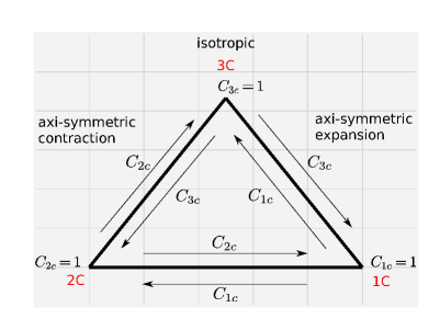
Figure 1: The barycentric map with the one-, two- and three-component corners, and the variation of its coefficients. Arrows indicates directions along which the corresponding coefficient linearly decreases from one towards zero.

3 Reynolds stress perturbation

3.1 Anisotropy tensor decomposition

The eigen decomposition of the anisotropy tensor reads

$$b_{ij}=v_{ik}\Lambda_{kl}v_{jl},$$ (14)

where $v_{ij}$ are the eigenvectors and $\Lambda_{ij}:=\mathrm{diag}\left(\lambda_{1},\lambda_{2},\lambda_{3}\right)$ is the diagonal matrix of eigenvalues. Hence, the Reynolds stress tensor can be written as

$$\overline{u^{\prime}_{i}u^{\prime}_{j}}=2k\left(\frac{1}{3}\delta_{ij}+v_{ik}\Lambda_{kl}v_{jl}\right)$$ (15)

Here, the turbulent kinetic energy, eigenvectors and eigenvalues represent the magnitude, orientation and shape of the Reynolds stress respectively. In (Mishra et al., 2016), the authors have attempted to quantify the uncertainty in RANS closures due to coarse graining, to guide the perturbations to the turbulent kinetic energy. For an approach perturbing the eigenvectors $v_{ij}$, see (Mishra & Iaccarino, 2016).

Emory et al. (2011) used Eq. (15) to perturb the baseline Reynolds stress tensor by replacing the eigenvalue matrix $\Lambda_{ij}$ with a perturbed matrix $\Lambda^{*}_{ij}$. Starting from the baseline result in the barycentric map, perturbations were made towards the three corners of the barycentric map. At these new locations the perturbed tensor $\Lambda^{*}_{ij}$ could be calculated through Eq. (12). This resulted in three additional code evaluations, the result of which were used to bound the QoI based on the limiting states of componentality. To determine where in the spatial domain the perturbations should be applied, specialized sensors based on wall-distance (Emory et al., 2011) or streamline curvature (Gorlé et al., 2012) were developed to flag regions where the turbulence model assumptions were most likely to be invalid. Within those regions flagged by the sensors, the perturbations in the direction of the corners were either homogeneous and user-specified or determined by a separate model, e.g., an error model based on log-normal distributions of observed discrepancies between RANS and DNS. We refer to (Emory et al., 2013) for more details.

3.2 Invariant transport model

The aim of the current article is to perturb the eigenvalues of $b_{ij}$ in a more general fashion, representative of spatial features without the use of separate sensors. To this end, we define two additional model transport equations for the invariant coefficients $C_{1c}$ and $C_{2c}$. Transport equations for tensor invariants of $b_{ij}$ already exist in the context of return-to-isotropy models. For instance, in the case of decaying homogeneous anisotropic turbulence, Rotta’s model (Rotta, 1951) can be used as a starting point to arrive at the following equation for the evolution of the tensor invariants of $b_{ij}$ of Eq. (3)

$$\frac{\mathrm{d}b^{n}_{ii}}{\mathrm{d}t}=-n\left(C_{R}-1\right)\frac{\varepsilon}{k}b^{n}_{ii},$$ (16)

where $C_{R}=1.8$ (Pope, 2000).

However, we deal with a baseline eddy viscosity model which can be erroneous at certain locations, but which is able to yield accurate predictions outside these regions. Therefore, the transport equations for $C_{1c}$ and $C_{2c}$ should describe a return-to-eddy-viscosity when the Boussinesq hypothesis is expected to be valid.

A class of turbulence models which does so includes the LAG-type models (Olsen & Coakley, 2001), (Lillard et al., 2012), which add extra transport equations to account for non-equilibrium effects. Generally speaking, a flow is in equilibrium when the turbulent time scale is much smaller than the mean flow time scale, allowing the turbulence to react quickly to changes in the mean flow. In these types of circumstance, a direct proportionality between the Reynolds stress tensor and the mean strain rate is a reasonable assumption. However, when this is not the case, there is a lag in the response of the turbulence to changes in the mean flow. This lag cannot be accounted for by eddy-viscosity models since $\overline{u^{\prime}_{i}u^{\prime}_{j}}$ reacts immediately to changes in $S_{ij}$. To rectify this behavior, Lillard et al. (2012) add the following six transport equations

$$\frac{\mathrm{D}\overline{u^{\prime}_{i}u^{\prime}_{j}}}{\mathrm{D}t}=a_{0}\frac{\epsilon}{k}\left(\overline{u^{\prime}_{i}u^{\prime}_{j}}^{\left(bl\right)}-\overline{u^{\prime}_{i}u^{\prime}_{j}}\right),$$ (17)

where $\overline{u^{\prime}_{i}u^{\prime}_{j}}^{(bl)}$ is the baseline Reynolds stress tensor computed with the Boussinesq hypothesis. The central idea of Eq. (17) is to modulate the six components of $\overline{u^{\prime}_{i}u^{\prime}_{j}}$, such that the turbulence model no longer responds too rapidly to changes in the mean flow. Along a steamline, a $\overline{u^{\prime}_{i}u^{\prime}_{j}}$ component goes to its baseline value with a time scale $\epsilon/k$ computed from the underlying baseline model.

The rate of the return to eddy viscosity can thus be controlled by the value of $a_{0}$, for which the proposed value is 0.35 (Olsen & Coakley, 2001). As is the case with most turbulence models, this value is ad hoc and not supported by theory. In (Lillard et al., 2012), the model response is evaluated at two different values of $a_{0}$, but validated only on flat-plate experimental velocity data. Moreover, it was recently argued in (Spalart, 2015) that equilibrium is not a well defined concept, and that near the wall the deep anisotropy is the cause of RANS model failure, rather than a lag in the response to changes in $S_{ij}$. In any case, here we use the ideas of Eqs. (16)-(17) to perturb the solution away from the Boussinesq hypothesis, possibly towards a more anisotropic state, in a low-dimensional fashion. To that end, we propose the following model transport equations for $C_{1c}$ and $C_{2c}$:

$$\frac{\mathrm{D}C_{1c}}{\mathrm{D}t}=a_{1c}\frac{\epsilon}{k}\left(C_{1c}^{(bl)}-C_{1c}\right)+\frac{\partial}{\partial x_{i}}\left((\nu+\frac{\nu_{T}}{\sigma_{1c}})\frac{\partial C_{1c}}{\partial x_{i}}\right)$$

$$\frac{\mathrm{D}C_{2c}}{\mathrm{D}t}=a_{2c}\frac{\epsilon}{k}\left(C_{2c}^{(bl)}-C_{2c}\right)+\frac{\partial}{\partial x_{i}}\left((\nu+\frac{\nu_{T}}{\sigma_{2c}})\frac{\partial C_{2c}}{\partial x_{i}}\right).$$ (18)

The $C^{(bl)}_{1c}$, $C^{(bl)}_{2c}$ are the coefficients computed using the eigenvalues of the Boussinesq anisotropy tensor, i.e., from

$$b^{(bl)}_{ij}=-\frac{\nu_{T}}{k}S_{ij}.$$ (19)

We will not commit to a single value for the coefficients of the LAG term (as optimal values are likely to be flow dependent (Edeling et al., 2014)), and instead consider a range of coefficients. Furthermore, we will examine the effect of lagging one equation more than the other in order to cover a wider area in the barycentric map, thereby incorporating more of the uncertainty in the eigenvalues of $b_{ij}$.

We define the boundary conditions following an approach similar to the original LAG model (Olsen & Coakley, 2001). At a solid smooth wall, we set the values of $C_{1c}$ and $C_{1c}$ equal to the baseline values $C^{(bl)}_{1c}$ and $C^{(bl)}_{2c}$. If the turbulence model equations are integrated down to the wall using damping functions, this essentially sets the values equal to zero. However, if wall functions are used, non-zero values of $C_{1c}$ and $C_{2c}$ are obtained. At an inflow boundary, it is assumed that the freestream turbulence is isotropic, i.e., $\overline{u^{\prime}_{i}u^{\prime}_{j}}={2}/{3}k_{\infty}\delta_{ij}$, yielding $C_{1c}=C_{2c}=0$. Outflow boundary values are extrapolated from internal cells.

The decision of where, how much and in what direction to perturb the eigenvalues of $b_{ij}$ is now determined by Eq. (18), and does not require any user input besides the specification of the coefficients $a_{1c}$, $a_{2c}$, $\sigma_{1c}$ and $\sigma_{2c}$. In cases where the left-hand side of Eq. (18) is zero (e.g., a quasi one-dimensional boundary layer), the diffusion term is needed to obtain a result different from the baseline state. Otherwise, one might choose to neglect this term, in line with the orginal LAG model. For now we include diffusion, but our focus is on the effect of the LAG term. As will be discussed in Section 3.3, writing transport equations for the barycentric coefficients rather than the Reynolds stresses yields a model that behaves intuitively with the choice of LAG coefficients $a_{1c}$ and $a_{2c}$. Also, since we keep the closure coefficients of the underlying baseline model fixed, these LAG coefficients are the only unknowns. Determining the effect of these coefficients on the QoI constitutes a low-dimensional UQ problem for which many off-the-shelf techniques exist, e.g. stochastic collocation or polynomial chaos methods (Eldred & Burkardt, 2009).

3.3 Effect of LAG coefficients

We specify the default values of the coefficients in (18) as

$$a_{1c}=a_{2c}=0.35\quad\quad\sigma_{1c}=\sigma_{2c}=1.0.$$ (20)

As previously explained, these are ad hoc choices and we do not claim universality on these values. The lag coefficients $a_{1c}$ and $a_{2c}$ determine the rate of return to eddy viscosity. Higher values result in $C_{1c}$ or $C_{2c}$ distributions that more closely follow the Boussinesq result. Let us define three cases that represent limiting trajectories:

1. $a_{1c}=a_{2c}=0.35$,

2. $a_{1c}=0$, $a_{2c}=0.35$,

3. $a_{1c}=0.35$, $a_{2c}=0$.

The resulting trajectories in the barycentric map, computed on a flat plate case, are shown in Figure 2. Before discussing these results, let us first note that the unperturbed baseline result will lie on top of the plane strain line for this flow case. A model will follow the plane strain turbulence line when at least one eigenvalue of $b_{ij}$ is zero (Banerjee et al., 2007).

When $a_{1c}=a_{2c}$ (case 1), both transport equations in Eq. (18) return to the Boussinesq solution at the same rate. As a result, the trajectory in the barycentric map still lies along the plane strain line (see Figure 2). Along this line the distribution is different than that of the unperturbed model, depending on the values of $a_{1c}$ and $a_{2c}$.

To observe larger deviations from the results of the baseline model, unequal LAG coefficients are required. In the second limiting case we enforce a homogeneous solution $C_{1c}=0$ by setting $a_{1c}=0$. This forces the trajectory to follow the axi-symmetric contraction border (see again Figure 2). Similarly, setting $a_{2c}=0$ results in a trajectory along the axi-symmetric expansion border, where $C_{2c}=0$.

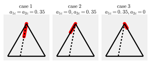
Figure 2: The trajectories in the barycentric map of the three coefficient cases. The dashed line denotes the plane strain line where $\lambda_{2}=0$.

3.4 Model behavior at 3C

When $a_{1c}=a_{2c}=0.0$, all points in the flow domain will be confined to the 3C corner of the barycentric map. The behavior of the model in this limit will be determined by the representation of the production term in the $k$ equation. The exact production term reads

$$\mathcal{P}:=-\rho\overline{u^{\prime}_{i}u^{\prime}_{j}}\frac{\partial\bar{u}_{i}}{\partial x_{j}},$$ (21)

which is modeled as $\mathcal{P}:=\rho\nu_{T}\left({\partial\bar{u}_{i}}/{\partial x_{j}}\right)^{2}$ in the $k-\varepsilon$ model (Wilcox, 1998). If the perturbed Reynolds stress tensor is used in Eq. (21), the flow becomes laminar when all points are perturbed to the 3C corner (since the off-diagonal component is the dominant contribution to $\mathcal{P}$ in this case). If the modeled production term is retained, the flow becomes isotropic with non-zero $k$. Employing the latter option has a number of advantages. First, from a UQ perspective one might be interested in the uncertainty of a given baseline model, and will therefore not alter the mathematical form of this model before performing the UQ analysis. Second, laminarizing the flow can lead to convergence issues. For investigating the behavior of model Eq. (18), we wish to retain the ability of perturbing all the way to the 3C corner, and hence we keep the Boussinesq production term. That said, it should be noted that when one relaxes this requirement, the use of Eq. (21) can improve the $k$ predictions (Gorlé et al., 2012).

3.5 Spatial distribution of perturbations

The extend of baseline model failure will depend upon the local flow physics, (see e.g., (Ling & Templeton, 2015)) for a detailed discussion of localized RANS failure. Ideally, the location, magnitude and direction of the perturbations should reflect this non-uniform nature of the RANS error. As mentioned, one may employ specialized marker functions based on local flow features to restrict the perturbations to regions where failure of the baseline model can reasonably be expected (Emory et al., 2013), (Gorlé et al., 2012). Besides determining the magnitude and direction, the LAG term also doubles as a marker function which flags regions where the Boussinesq assumption is likely to be invalid (Lillard et al., 2012). As an example, consider the spatial distribution of $|\lambda_{1}-\lambda_{1}^{(eq)}|$ for a flat plate flow shown in Figure 3. Here, $\lambda_{1}^{(eq)}$ is the largest eigenvalue of Eq. (19). Only close to the wall do we find any significant departure from the Boussinesq value of the largest eigenvalue. Away from the wall, where the flow is essentially uniform, we find no perturbations.

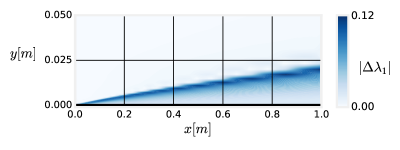
Figure 3: A contour plot of $|\Delta\lambda_{1}|:=|\lambda_{1}-\lambda_{1}^{(eq)}|$ for $a_{1c}=a_{2c}=0.35$.

3.6 Realizability

To obtain physically feasible values for the components of the Reynolds stress tensor, the realizability constraints first defined by (Schumann, 1977) must hold, i.e.

$$\overline{u^{\prime}_{\mu}u^{\prime}_{\mu}}\geq 0\quad\quad(\overline{u^{\prime}_{\mu}u^{\prime}_{\nu}})^{2}\leq\overline{u^{\prime}_{\mu}u^{\prime}_{\mu}}\;\overline{u^{\prime}_{\nu}u^{\prime}_{\nu}}\quad\quad\det\left(\overline{u^{\prime}_{i}u^{\prime}_{j}}\right)\geq 0,\quad\quad\mu,\nu\in\{1,2,3\}.$$ (22)

Besides constraints on the Reynolds stress tensor itself, it is also possible to derive constraints on the associated process of evolution, see (Mishra & Girimaji, 2014).

When Eq. (22) is satisfied, we are guaranteed non-negative diagonal components and correlations which do not exceed the limits imposed by the Cauchy-Schwarz inequality. If during the iteration of the turbulence model one of the diagonal components approaches zero, weak realizability constraints on its space and time derivative can be enforced in order to avoid negative values of this component (Pope, 1985). To see across which of the three boundaries of the barycentric map the transition from positive to negative $\overline{u^{\prime}_{\mu}u^{\prime}_{\mu}}$ can occur, consider the Reynolds stress tensor in its principal axes:

$$\widehat{u^{\prime}_{i}u^{\prime}_{j}}=\frac{2}{3}k\left(\begin{tabular}[]{ccc}$2C_{1c}+\frac{1}{2}{C_{2c}}+1$&0&0\\ 0&$-C_{1c}+\frac{1}{2}C_{2c}+1$&0\\ 0&0&$-C_{1c}-C_{2c}+1$\end{tabular}\right),$$ (26)

where Eqs. (5), (2) and (12) are used to express the diagonal components in terms of the coefficients. We now have

• axi-symmetric contraction: $C_{1c}=0\rightarrow\widehat{u^{\prime}_{3}u^{\prime}_{3}}=0$ at 2C,

• axi-symmetric expansion: $\;\;C_{2c}=0\rightarrow\widehat{u^{\prime}_{2}u^{\prime}_{2}}=0$ and $\widehat{u^{\prime}_{3}u^{\prime}_{3}}=0$ at 1C,

• two-component boundary: $\;C_{3c}=0\rightarrow$ $\widehat{u^{\prime}_{2}u^{\prime}_{2}}=0$ at 1C and $\widehat{u^{\prime}_{3}u^{\prime}_{3}}=0$ everywhere.

These results show that only along the bottom boundary, is the component $\widehat{u^{\prime}_{3}u^{\prime}_{3}}$ (corresponding to the smallest eigenvalue $\lambda_{3}$) zero, hence the name two-component boundary. Thus, when a principal Reynolds stress vanishes somewhere in the flow domain, the corresponding point in the barycentric map will be located at the bottom boundary. Depending on the sign of the temporal and spatial derivatives of this vanishing $\widehat{u^{\prime}_{\mu}u^{\prime}_{\mu}}$, the trajectory will either cross the boundary yielding unrealizable solutions, or move back into the barycentric map. To avoid the former, realizability constraints can be imposed on closure models. A convenient quantity to impose such constraints is

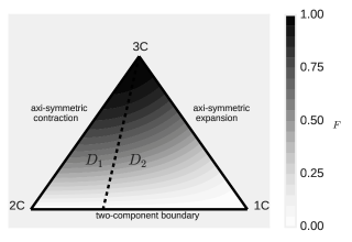
Figure 4: The barycentric map color coded according to (27). Domain $D_{1}$ and $D_{2}$ are the two sub triangles left and right of the plane strain line.

$$\widehat{F}:=\det\left(\frac{\widehat{u^{\prime}_{i}u^{\prime}_{j}}}{\frac{2}{3}k}\right)=\left(\frac{2}{3}k\right)^{-3}\cdot\widehat{u^{\prime}_{1}u^{\prime}_{1}}\cdot\widehat{u^{\prime}_{2}u^{\prime}_{2}}\cdot\widehat{u^{\prime}_{3}u^{\prime}_{3}},$$ (27)

which is defined such that $\widehat{F}=1$ in the case of isotropic turbulence and $\widehat{F}=0$ when a principal Reynolds stress vanishes. Thus, $\widehat{F}\geq 0$ holds inside the barycentric map (see Figure 4), which can be considered as a normalized version of the third condition in Eq (22). The condition of weak realizability ensures that an initially three-component state of turbulence can never achieve a two-component state, i.e., where the two-component boundary is made inaccessible through a constraint on the first derivative of $\widehat{F}$ (Pope, 1985):

$$\left.\frac{\mathrm{D}\widehat{F}}{\mathrm{D}t}\right|_{\widehat{F}=0}>0.$$ (28)

Using Eq. (26) to expand Eq. (27) yields

$$\widehat{F}=(2C_{1c}+\frac{1}{2}{C_{2c}}+1)(-C_{1c}+\frac{1}{2}C_{2c}+1)(-C_{1c}-C_{2c}+1)$$ (29)

After some algebra (using $C_{2c}=1-C_{1c}$ at the two-component boundary), we obtain

$$\left.\frac{\mathrm{D}\widehat{F}}{\mathrm{D}t}\right|_{\widehat{F}=0}=\left(\frac{9}{4}C_{1c}^{2}-\frac{9}{4}\right)\frac{\mathrm{D}C_{1c}}{\mathrm{D}t}+\left(\frac{9}{4}C_{1c}^{2}-\frac{9}{4}\right)\frac{\mathrm{D}C_{2c}}{\mathrm{D}t}.$$ (30)

At this point our transport model Eq. (18) for $C_{1c}$ and $C_{2c}$ is inserted into Eq. (30), and the weak realizability condition Eq. (28) then becomes

$$a_{1c}C_{1c}^{(bl)}+a_{2c}C_{2c}^{(bl)}\leq\left(a_{1c}-a_{2c}\right)C_{1c}+a_{2c},\quad\mathrm{when}\;\;\widehat{F}=0.$$ (31)

Under certain conditions described in Section 3.3, the results from a Boussinesq model will lie on top op the plane strain line. Along this line $C^{(bl)}_{2c}=2C^{(bl)}_{1c}$ holds, allowing us to simplify Eq. (31) further to

$$\left(a_{1c}+2a_{2c}\right)C_{1c}^{(bl)}\leq\left(a_{1c}-a_{2c}\right)C_{1c}+a_{2c},\quad\mathrm{when}\;\;\widehat{F}=0.$$ (32)

Consider the two domains $D_{1},D_{2}$ at either side of the plane strain line as shown in Figure 4. Let us evaluate the inequality Eq. (32) in both domains, starting with $D_{1}$. In this domain, $C_{1c}\in\left[0,1/3\right]$ along the two-component boundary. Each $C_{1c}$ is associated with a baseline value $C_{1c}^{(bl)}\in\left[0,1/3\right]$. Motivated by the results of Figure 2, we assume that points are pushed into this domain because we have selected the coefficients such that $a_{1c}<a_{2c}$. In this case inequality Eq. (32) is always satisfied (see Figure 5a). Moreover, even if $a_{1c}>a_{2c}$, Eq. (32) will still hold. Note that we assume both coefficients are positive.

In $D_{2}$, the range of the baseline coefficient is still $C_{1c}^{(bl)}\in\left[0,1/3\right]$, but $C_{1c}\in\left[1/3,1\right]$ along the two-component boundary. If a trajectory enters $D_{2}$ while $a_{1c}<a_{2c}$, the realizability condition Eq. (32) could be violated. However, the results of Figure 2 indicate that for $a_{1c}<a_{2c}$ the trajectories are pushed away from $D_{2}$. Hence, under the condition that $a_{2c}<a_{1c}$, Figure 5b shows that on this side of the plane strain line the model is also weakly realizable.

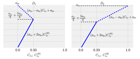
Figure 5: The lines of inequality Eq. (32) for $D_{1}$ (left, $a_{1c}<a_{2c}$) and $D_{2}$ (right, $a_{2c}<a_{1c}$).

To test the validity of realizability condition Eq. (32), consider a square duct case where the trajectories start at the 1C corner by setting the wall boundary conditions of model Eq. (18) equal to one-component turbulence. This is the most extreme case where two principal Reynolds stresses vanish. We then run the model under the two limiting axi-symmetric cases, i.e., cases 2 and 3 of Section 3.3. The preceding analysis suggests that in the latter case the model should still be realizable, whereas in the former case we can expect failure. The result are shown in Figure 6. Note that for case 3 the solution is indeed realizable, as the trajectory moves from the 1C to the 3C corner along the axi-symmetric expansion border. And as expected, case 2 displays a clear violation of realizability.

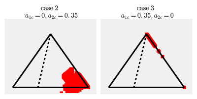
Figure 6: Model Eq. (18) computed on a square-duct flow. The boundary conditions were set to 1C turbulence, i.e., $C_{1c}=1$, $C_{2c}=0$ at the four walls of the duct.

3.7 Perturbation Bounds

Let us determine the possibility of a priori identifying the LAG coefficients $a_{1c}$ and $a_{2c}$ that will yield the maximum and minimum bound on the perturbed eigenvalues that can be achieved with model Eq. (18). To this end, we decompose the anisotropy tensor as

$$b_{ij}=b_{ij}^{(bl)}+v_{ik}\check{E}_{kl}v_{jl}.$$ (33)

Here, $\check{E}_{ij}$ represents the perturbation tensor and is given by $\check{E}_{ij}:=\mathrm{diag\left(\Delta\lambda_{1},\Delta\lambda_{2},\Delta\lambda_{3}\right)}$, where $\Delta\lambda_{\alpha}$ is the perturbation such that $\lambda_{\alpha}=\lambda^{(bl)}_{\alpha}+\Delta\lambda_{\alpha}$. Decomposition Eq. (33) is possible because $b_{ij}$, $b_{ij}^{(bl)}$ and $\check{E}_{ij}$ share the same eigenspace. Note that the superscript of $\check{E}_{ij}$ indicates that the increasing diagonal order found in $\hat{b}_{ij}$ might not be present in $\check{E}_{ij}$. Assuming again that the baseline model will follow the plane strain line in the barycentric map, $\check{E}_{ij}$ can be written as

$$\check{E}_{ij}=\left(\begin{tabular}[]{ccc}$\frac{2}{3}\left[C_{1c}-\frac{3}{2}C_{1c}^{(bl)}\right]+\frac{1}{6}C_{2c}$&0&0\\ 0&$-\frac{1}{3}C_{1c}+\frac{1}{6}C_{2c}$&0\\ 0&0&$-\frac{1}{3}\left[C_{1c}-3C_{1c}^{(bl)}\right]-\frac{1}{3}C_{2c}$\end{tabular}\right).$$ (37)

By fixing the baseline coefficient to an arbitrary value $C_{1c}^{(bl)}\in\left[0,1/3\right]$, we can plot the isocontours of the $\Delta\lambda_{\alpha}$ in order to identify the directions of maximum and minimum perturbation. The results are shown in Figure 7. Clearly, $\Delta\lambda_{1}$ is maximized in the direction of 1C, and minimized towards 3C. The perturbation $\Delta\lambda_{2}$ is maximized at 2C and minimized at 1C. Finally, the maximum of $\Delta\lambda_{3}$ is located at 3C, and its minimum is found anywhere along the 2C boundary. Thus, straight lines in the direction of minimum/maximum $\Delta\lambda_{\alpha}$ are the axi-symmetric expansion, contraction and the plane-strain line. Trajectories along these lines can be obtained with a priori known values for $a_{1c}$ and $a_{2c}$ (see Figure 2).

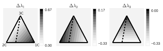
Figure 7: Isocontours of eigenvalue perturbations for a given value of $C_{1c}^{(bl)}$, which this case is set to zero.

4 Results

4.1 QoI Bounds

Let us consider a flat plate flow with a Reynolds number of $\mathrm{Re}=1.1\times 10^{6}$ based on the plate length. To examine the bounds on the QoIs resulting from using model Eq. (18), we construct a two-dimensional tensor product of LAG coefficient from one-dimensional Clenshaw-Curtis abscissas (see Figure 8). Next, we simply run the model on each $(a_{1c},a_{2c})$ combination and examine the possible range of solutions. Note that one could use the samples obtained in this way towards constructing a stochastic collocation model (Witteveen et al., 2009).

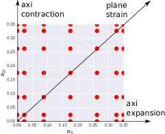
Figure 8: A tensor product of 1D Clenshaw-Curtis abscissas $a_{\alpha c}=-\cos\frac{(j-1)\pi}{m-1}$, $j=1,\cdots,m$. The considered 1D range is $\left[0,0.35\right]$.

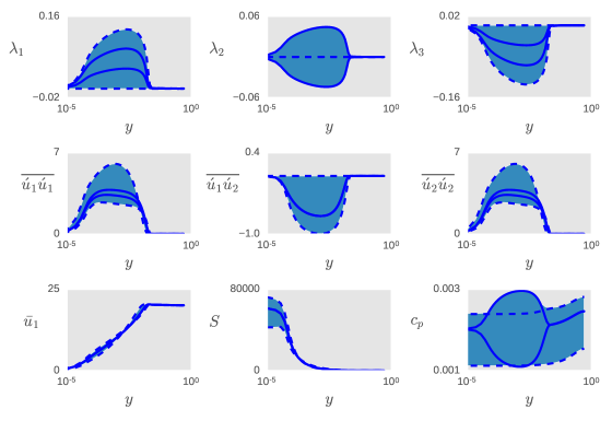
Figure 9: The three anisotropy eigenvalues, Reynolds-stress components, mean streamwise velocity, mean strain-rate magnitude ($S:=\sqrt{S_{ij}S_{ji}}$) and the pressure coefficient versus the wall-normal direction in log scale, at streamwise location $x=0.8$. The dashed lines are the solutions at the opposite ends along the plane-strain line (computed using $(0,0)$ and $(0.35,0.35)$), and the solid lines denote the axi-symmetric profiles ($(0,0.35)$ and $(0.35,0)$).

The results are shown in Figure 9. Notice that most QoI are bounded by a plane-strain bound, denoted by the dashed lines. The first exception is $\lambda_{2}$, which is zero along the plane-strain line by definition. Instead, $\lambda_{2}$ is bounded by the axi-symmetric profiles. Moreover, these profiles are symmetric around $\lambda_{2}=0$. The other exception is the pressure coefficient $c_{p}:={(p-p_{\infty})}/{(\rho V_{\infty}^{2}/2)}$ (in wall-normal direction), which is bounded by both the plane-strain and axi-symmetric results.

Let us reiterate here that the bounds of Figure 9 are a representation of the uncertainty in the shape of $\overline{u^{\prime}_{i}u^{\prime}_{j}}$ only. To inject additional uncertainty into the problem, perturbations in the orientation of the Reynolds stress tensor should be included (see, e.g., (Mishra & Iaccarino, 2016)).

5 Conclusions

We introduced two model transport equations for the coefficients of the barycentric map to find intervals due to epistemic model-form uncertainty in RANS closures. The output of this model is used to compute spatially varying perturbations of the eigenvalues of the anisotropy tensor. By incorporating so-called LAG terms, these perturbations are made with respect to a baseline eddy-viscosity model, such that in certain areas the results of this underlying model are recovered. The global behavior of the discrepancy model is governed by two LAG coefficients, the difference in which determines the amount of perturbation from the baseline state. In which direction of the barycentric map the perturbations are made is determined by the sign of the difference. Moreover, weak realizability conditions and bounds for the eigenvalue perturbations can also be associated with certain a priori known values of the LAG coefficients. This association results in an intuitive discrepancy model, amenable to physical reasoning.

When applying the model to a turbulent flat plate flow, we found that the Quantities of Interest (QoIs) are bounded by the same a priori known coefficient values. Note that we make no claim as to the generality of this result. Future work will involve computing other flow cases, as well as a Bayesian analusys in order to find stochastic (posterior) estimates of the LAG coefficients and QoIs. Thus, the results of this paper can be considered as a first step towards a full Bayesian description of the uncertainty in the eigenvalues, in the sense that it describes the effects of (uniform) prior distributions on the model coefficients. A further reseach option for the future is the investigation of non-linear return to eddy viscosity models.

References

- Banerjee et al. (2007) Banerjee, S., Krahl, R., Durst, F. & Zenger, C. 2007 Presentation of anisotropy properties of turbulence, invariants versus eigenvalue approaches. J. Turb. 8, N32.
- Edeling et al. (2014) Edeling, W. N., Cinnella, P., Dwight, R. P. & Bijl, H. 2014 Bayesian estimates of parameter variability in the k– turbulence model J. Comput. Phys., 258, 73–94.
- Eldred & Burkardt (2009) Eldred, M.S. & Burkardt, J. 2009 Comparison of non-intrusive polynomial chaos and stochastic collocation methods for uncertainty quantification AIAA paper 2009-976.
- Emory et al. (2011) Emory, M., Pecnik, R. & Iaccarino, G. 2011 Modeling structural uncertainties in Reynolds-averaged computations of shock/boundary layer interactions, AIAA Paper 2011-479.
- Emory et al. (2013) Emory, M., Larsson, J. & Iaccarino, G. 2013 Modeling of structural uncertainties in Reynolds-averaged Navier-Stokes closures Phys. Fluids., 25, 110822.
- Gorlé et al. (2012) Gorlé, C., Emory, M., Larsson, J. & Iaccarino, G. 2012 Epistemic uncertainty quantification for RANS modeling of the flow over a wavy wall Annual Research Briefs, Center for Turbulence Research, Stanford University, 81–91.
- Lay (2006) Lay, D. C. Linear algebra and its applications Pearson/Addison-Wesley, 2006.
- Lillard et al. (2012) Lillard, R.P., Oliver, A.B., Olsen, M.E., Blaisdell, G.A. Lyrintzis, A.S. 2012 The lagRST model: a turbulence model for non-equilibrium flows, AIAA Paper 2012-0444.
- Ling & Templeton (2015) Ling, J. & Templeton, J., 2015 Evaluation of machine learning algorithms for prediction of regions of high Reynolds averaged Navier Stokes uncertainty Phys. Fluids., 27, 085103.
- Lumley & Newman (1977) Lumley, J. L. & Newman, G. R. 1977 The return to isotropy of homogeneous turbulence J. Fluid. Mech. 82, 161–178.
- Mishra & Girimaji (2014) Mishra, A. & Girimaji, S. 2014 On the realizability of pressure-strain closures, J. Fluid Mech., 755, 535–560.
- Mishra & Iaccarino (2016) Mishra, A. & G. Iaccarino 2016 RANS predictions fo high-speed flows using enveloping models, Annual Research Briefs, Center for Turbulence Research, Stanford University.
- Mishra et al. (2016) Mishra, A., Iaccarino, G., & Duraisamy, K. 2016 Sensitivity of flow evolution on turbulence structure, Phys. Rev. Fluids, 1, 052402.
- Olsen & Coakley (2001) Olsen, M.E. & Coakley, T.J. 2001 The lag model, a turbulence model for non equilibrium flows AIAA Paper 2001-2564.
- Pope (1985) Pope, S. B. 1985 PDF methods for turbulent reactive flows Prog. Energy Combust. Sci., 11, 119–192
- Pope (2000) Pope, S. B. Turbulent Flows. IOP Publishing, 2000.
- Rotta (1951) Rotta, J. C. 1951 Statistische Theorie nichthomogener Turbulenz Z. Phys., 129, 547–572.
- Schumann (1977) Schumann, U. 1977 Realizability of Reynolds-stress turbulence models Phys. Fluids, 20, 721–725.
- Spalart (2015) Spalart, P. R 2015 Philosophies and fallacies in turbulence modeling Prog. Aerosp. Sci., 74, 1–15.
- Wilcox (1998) Wilcox, D. C. 1998 Turbulence Modeling for CFD. DCW Industries.
- Witteveen et al. (2009) Witteveen, J.A.S., Doostan, A., Pecnik, R. & Iaccarino, G. 2009 Uncertainty quantification of the transonic flow around the RAE 2822 airfoil Annual Research Briefs, Center for Turbulence Research, Stanford University, pp 93-104.
- Wu et al. (2016) Wu, J., Wang, J. and Xiao, H. & Ling, J. 2016 Physics-informed machine learning for predictive turbulence modeling: A priori assessment of prediction confidence, arXiv preprint arXiv:1607.04563.
- Zhang & Duraisamy (2015) Zhang, Z. J. & Duraisamy, K. 2015 Machine learning methods for data-driven turbulence modeling, AIAA Paper 2015-2460.