Electrostatic and induction effects in the solubility of water in alkanes

Abstract

Experiments show that at 298 K and 1 atm pressure the transfer free energy, $\mu^{\rm ex}$, of water from its vapor to liquid normal alkanes $C_{n}H_{2n+2}$ ($n=5\ldots 12$) is negative. Earlier it was found that with the united-atom TraPPE model for alkanes and the SPC/E model for water, one had to artificially enhance the attractive alkane-water cross interaction to capture this behavior. Here we revisit the calculation of $\mu^{\rm ex}$ using the polarizable AMOEBA and the non-polarizable Charmm General (CGenFF) forcefields. We test both the AMOEBA03 and AMOEBA14 water models; the former has been validated with the AMOEBA alkane model while the latter is a revision of AMOEBA03 to better describe liquid water. We calculate $\mu^{\rm ex}$ using the test particle method. With CGenFF, $\mu^{\rm ex}$ is positive and the error relative to experiments is about 1.5 $k_{\rm B}T$. With AMOEBA, $\mu^{\rm ex}$ is negative and deviations relative to experiments are between 0.25 $k_{\rm B}T$ (AMOEBA14) and 0.5 $k_{\rm B}T$ (AMOEBA03). Quantum chemical calculations in a continuum solvent suggest that zero point effects may account for some of the deviation. Forcefield limitations notwithstanding, electrostatic and induction effects, commonly ignored in considerations of water-alkane interactions, appear to be decisive in the solubility of water in alkanes.

I Introduction

Alkane solubility in water is of fundamental importance in understanding various self-assembly processes and of the nature of water itself Stillinger (1980); Hummer et al. (1998); Chandler (2005). This process has been studied extensively over the last few decades both experimentally and in computer simulations. The converse process, the solubility of water in alkanes, has received considerably less attention. Nevertheless, understanding the solubility of water in alkanes is also of fundamental scientific and technological interest. Technologically, one encounters the problem of characterizing water solubility in alkanes in all aspects related to water in oil and oil-related products. Scientifically, this problem challenges our appreciation of the intermolecular forces between alkane, a nonpolar substance, and water, a prototypical polar compound. The present paper is motivated by these scientific and technological considerations.

In discussions of alkane solubility in water, the emphasis is typically on the thermodynamics of creating a cavity in the liquid Hummer et al. (1998); Chandler (2005), with the different physical ingredients of the attractive interaction between the alkane and the water lumped into a single alkane-water dispersion interaction. Usually the dispersion interaction is modeled using the Lennard-Jones potential with the Lorentz-Berthelot mixing rule. In many instances it has often been found necessary to enhance the alkane-water attractive interaction over that based on using the Lorentz-Berthelot mixing rule (for example, see Refs. Docherty et al. (2006); Ashbaugh et al. (2010)), an approach that is rationalized as a way to account for the physics of polarizability, if polarizability is not explicitly considered. The idea of non-negligible electrostatic interaction between an alkane and water is almost never considered, but quantum chemical calculations Akin-Ojo and Szalewicz (2005) do suggest that the bonding between methane, a prototypical hydrophobe, and water, in specific configurations can even be characterized as “weak” hydrogen bonding.

Recently, Ballal et al. Ballal et al. (2014, 2016) investigated the solubility of water in alkanes using molecular simulations. In their approach they used the united atom TraPPE Martin and Siepmann (1998) model of alkanes and the SPC/E Berendsen et al. (1987) model for water. They found that with the Lorentz-Bertholet mixing rule for the alkane-water cross-interaction, the predicted transfer free energy of water to alkanes $C_{n}H_{2n+2}$ ($n=5\ldots 12$) was much too positive. To recover the experimentally observed fraction of water in alkanes they had to increase the water-alkane attractive interaction. Ballal et al. Ballal et al. (2014) considered several physical explanations for the enhanced effective attraction, but a compelling explanation for the observed solubility of water in alkanes is still wanting. As McDaniel and Yethiraj McDaniel and Yethiraj (2016) subsequently noted in an insightful comment, the work by Ballal et al.Ballal et al. (2014) “uncovered a wonderful example of where pure-component parameters fail for mixtures” and “a more accurate model must better describe the electrostatic, induction, and dispersion interactions, all of which are potentially important.” Recent studies on water/CO₂ and water/n-alkane mixtures further support this idea Jiang et al. (2017).

Here we revisit the problem of water solubility in alkanes using the polarizable AMOEBA Ren and Ponder (2003); Laury et al. (2015); Ren et al. (2011) all-atom forcefield. An important feature of the AMOEBA model is extensive reliance on ab initio calculations on small clusters during the parameter development. Further the electrostatic interactions are based on distributed multipoles, which are well known to encode a high level of chemical realism Stone (2013). Having a better description of the electric field around the molecule is also expected to better describe the physics of induction. On the basis of such a model, we find that both electrostatics and induction effects play a decisive role in describing the solubility of water in alkanes.

II Theory

II.1 Analysis of experimental data

The experimental results Polak and Lu (1973); Roddy and Coleman (1968); Schatzberg (1963) of the solubility of water in alkanes are reported as a mole fraction ($x_{w}$) or p.p.m. by weight. The alkanes are at 298.15 K, and while it is not explicitly stated, one can infer from the experimental procedure that the pressure is 1 atm. For the temperature and pressure conditions, the pure alkane density is well established and we obtain those values from the NIST database Lemmon et al. (2017).

Let the number density of neat alkane be $\rho_{a}$. Since the mole fraction of water in alkane is of the order of 10^-4, to an excellent approximation the number density of water in the alkane phase is $\rho_{w}^{(a)}=x_{w}\cdot\rho_{a}$. (In this limit, the p.p.m. measure is also readily converted to $x_{w}$.) At 298.15 K, using the pressure-volume data from the NIST database Lemmon et al. (2017), an estimate of the Poynting pressure correction shows that the chemical potential of water at 1 atm. pressure and 298.15 K is only about 0.001 kcal/mol higher than that at saturation. Hence for simplicity we will assume saturation conditions. Since the alkane solubility in water is also low, we assume that the chemical potential of water in the water-rich phase is the same as that of neat liquid water. Equating the chemical potential of water in the alkane-rich and liquid-water phases we have

$$\beta[\mu^{\rm ex}_{w|a}-\mu^{\rm ex}_{w|l}] = \ln\frac{\rho_{w}^{(l)}}{\rho_{w}^{(a)}}=\ln\frac{\rho_{w}^{(l)}}{x_{w}\cdot\rho_{a}}\,.$$ (1)

$\beta=1/k_{\rm B}T$, where $k_{\rm B}$ is Boltzmann’s constant, is the reciprocal temperature in energy units. $\mu^{\rm ex}_{w|l}$ is the excess chemical potential of water in liquid water and $\mu^{\rm ex}_{w|a}$ is the corresponding quantity in the alkane. The excess chemical potential collects all contributions due to intermolecular interactions and is the quantity of principal interest here. Please note that mass dependent effects are implicitly considered when we use experimental densities on the right hand side of Eq. 1. Within classical statistical mechanics, we assume mass dependent contributions cancel in composing the difference on the left hand side of Eq. 1. (We return to this point when we consider possible corrections due to quantization of nuclear motion.)

Analogous to Eq. 1,

$$\beta[\mu^{\rm ex}_{w|l}-\mu^{\rm ex}_{w|v}] = \ln\frac{\rho_{w}^{(v)}}{\rho_{w}^{(l)}}$$ (2)

gives the free energy to transfer water from its saturated vapor to the saturated liquid. Thus, from Eqs. 1 and 2, the free energy to transfer water from its vapor to the alkane is

$$\beta[\mu^{\rm ex}_{w|a}-\mu^{\rm ex}_{w|v}]=\ln\frac{\rho_{w}^{(v)}}{x_{w}\cdot\rho_{a}}\,.$$ (3)

All the quantities on the right hand side of Eq. 3 are known experimentally, and thus $\beta[\mu^{\rm ex}_{w|a}-\mu^{\rm ex}_{w|v}]$, which is the target of molecular simulations, is also well-characterized.

For the temperature and pressure under consideration, the water vapor can be treated as an ideal gas, i.e. $\beta\mu^{\rm ex}_{w|v}=0$. To confirm this please note that to the lowest order in density $\beta\mu^{\rm ex}_{w|v}=2B_{2}\rho_{w}^{(v)}\approx-3\times 10^{-3}$, where $B_{2}=-1160$ cm³/mol Harvey and Lemmon (2004) is the experimentally determined second virial coefficient of water at 298.15 K. We explicitly note the second virial correction anticipating our discussion below on the possible role of dimerization of water in the alkane.

II.2 Calculation of $\mu^{\rm ex}_{w|a}$

From the potential distribution theorem Widom (1982); Paulaitis and Pratt (2002); Beck et al. (2006); Pratt and Asthagiri (2007) we have

$$\beta\mu^{\rm ex}_{w|a}=-\ln\langle\langle e^{-\beta\Delta U}\rangle\rangle_{0}\,.$$ (4)

$\Delta U=U_{n+1}-U_{n}-U_{1}$ is the binding energy of the test particle indicated by ‘1’. $U_{n}$ is the potential energy of the neat solvent, $U_{n+1}$ is the potential energy of the neat solvent plus the added solute (water), and $U_{1}$ is the potential energy of the test particle. The outer-average $\langle\ldots\rangle_{0}$ indicates that the solvent and solute are thermally uncoupled and the inner-average $\langle\ldots\rangle$ indicates sampling over the conformations of the solute uncoupled from the solvent.

For the solvation of the rigid TIP4P/2005 Abascal and Vega (2005) water, we have only a single conformation to consider. In the case of water modeled by the AMOEBA forcefield, sampling over solute conformations is, in principle, required. However, estimation of bond and angle fluctuations from the known force constants suggests that to an excellent approximation using the equilibrium conformation of the isolated AMOEBA water is adequate. (Importantly, the binding energy calculations are expected to be insensitive to the tiny changes in the solute conformation.) Finally we note that a direct application of Eq. 4 always requires care. Here the free energies of interest are all within about $\pm 2$ k${}_{\rm B}T$ (see below), and we expect a direct application of Eq. 4 to ensure statistically converged results. Our results below support this expectation.

III Methods

III.1 Simulations

We study the solvation of TIP4P/2005 water in normal alkanes $C_{n}H_{2n+2}$ ($n=5\ldots 12$) modeled using CGenFF, the CHARMM General Forcefield Vanommeslaeghe et al. (2010), and the solvation of AMOEBA water Ren and Ponder (2003); Laury et al. (2015) in alkanes modeled by the AMOEBA forcefield Ren et al. (2011). For the temperature of 298.15 K and 1 atm pressure, we obtained the density of the alkanes from the NIST database (Table 1). We built reference structures for $C_{n}H_{2n+2}$ ($n=5\ldots 12$) using Avogadro Hanwell et al. (2012) and then using Packmol Martinez et al. (2009) packed $N$ (Table 1) of the alkane molecules in a cubic box to achieve the prescribed density. This system defined the starting configuration.

Table 1: Simulation cell density and number of particles. The density $\rho_{a}$ is obtained from the NIST database Lemmon et al. (2017). $N$ is the number of molecules in the system.

Species	$\rho_{a}$ (mol/l)	$N$
C5H12	8.6048	332
C6H14	7.5982	293
C7H16	6.7823	261
C8H18	6.1129	236
C9H20	5.5677	215
C10H22	5.1063	196
C12H26	4.3780	169

For simulations with the CGenFF forcefield, we use the NAMD Phillips et al. (2005) program. The starting simulation cells are energy minimized and then subjected to over 1 ns of equilibration under constant $NVT$ conditions. The temperature of 298.15 K is maintained using a Langevin thermostat. During this equilibration phase, the bond between the hydrogen and the parent heavy atom was held fixed and the time step for integrating the equations of motion was 2 fs. (The final configuration from this phase was subsequently used as a starting point for simulation using AMOEBA.) In the next phase, to allow a clear comparison with the simulations using AMOEBA, we remove the bond constraints on the hydrogens and equilibrate the system over 0.5 ns with 1 fs time step. Finally in the production phase that lasted 1 ns, we archive configurations every 100 fs to harvest 10000 configurations in all. The Lennard-Jones interactions are terminated at 14 Å by smoothly switching to zero starting at 13 Å. (Consistent with the forcefield model Vanommeslaeghe et al. (2010), we do not include any additional long-range LJ corrections.) Long-range electrostatic interactions are treated using particle mesh Ewald summations with a real space cutoff of 13 Å and a grid size of 0.5 Å for the reciprocal space sum.

For simulations with the AMOEBA forcefield, we use the TINKER molecular modeling package Ponder (2015). We use the Andersen thermostat to maintain the temperature and use a time step of 1 fs for integrating the equations of motion. The van der Waals interactions are terminated at 13 Å by smoothly switching to zero starting at 12 Å. (Once again, long-range LJ corrections are not included.) Long-range electrostatic interactions are treated using Ewald summations with a real space cutoff of 13 Å. Because of computational limitations the equilibration and production times varied among the various systems. Equilibration (production) times were as follows: C5, 62.3 ps (124.3 ps); C6, 58.8 ps (113.0 ps); C7, 56 ps (116.5 ps); C8, 51.5 ps (118 ps); C9, 51.5 ps (124 ps); C10, 51.5 ps (93 ps); and C12, 51.5 ps (85.8 ps). During the production phase, configurations were saved every 250 fs for analysis.

III.2 Test particle calculations

The test particle calculations are performed in two steps. First, in each of the archived frames, we lay a cubic grid of points and accept the point as a viable insertion site if the closest distance between the point and the nearest heavy atom is greater than 2.9 Å. (We note that even by 3.0 Å, the methane-water interactions become repulsive, indicating substantial overlap between the molecules Asthagiri et al. (2008).) This set of accepted points is saved. For calculations with the AMOEBA model, we separately calculate the energy of the water molecule $U_{1}$ and save it for subsequent use. For a given frame we first find the total energy of the system ($U_{n}$). Then we consider each of the viable insertion sites and write out new configuration files with both the alkane and inserted water coordinates. We then run an energy calculation using TINKER to obtain the energy of the complex $U_{n+1}$ and calculate $\Delta U$ (Eq. 4) for further analysis.

A similar procedure was followed for configurations obtained using CGenFF. However, for the test energy calculations, it proves more efficient to calculate $\Delta U$ using our in-house program. For long-range electrostatics we use the generalized reaction field Hummer et al. (1992); Hummer and Soumpasis (1994); Hummer et al. (1994) procedure for computational economy. (Test calculations with Ewald summations showed that the binding energy values using GRF and Ewald are the same to better than two decimal accuracy.)

For simulations with AMOEBA we attempt 2197 insertions per configuration for a total of between $0.7\times 10^{6}$ (C12) to $1.1\times 10^{6}$ (C5) trial points. Note that for the given sample size, the most positive free energy we can estimate is about 13 $k_{\rm B}T$($=\ln 1.1\times 10^{6}$), a number that is substantially larger than the largest positive value encountered in this work. (Hence we expect good statistical convergence.) Since we had many more frames with CGenFF, we only sample 343 points per configuration for a total of about $3\times 10^{6}$ trial points. For statistical analysis, we treat $\langle e^{-\beta\Delta U}\rangle_{0}$ obtained per frame as a random variable. Using the Friedberg-Cameron algorithm Allen and Tildesley (1987); Friedberg and Cameron (1970) we then obtain the mean across the entire sample (of frames) and the statistical inefficiency of the sampling. From this information, and using standard variance propagation rules, we calculate the $\beta\mu^{\rm ex}_{w|a}=-\ln\langle e^{-\beta\Delta U}\rangle_{0}$ and the associated standard error of the mean.

IV Results and Discussion

IV.1 Methane-water pair potential

Figure 1 shows the methane-water pair interaction using different forcefields. The reference values are based on symmetry adapted perturbation theory (SAPT) results published in Ref. Akin-Ojo and Szalewicz, 2005. Calculations using Gaussian09 Frisch et al. at the MP2-level with aug-cc-pVTZ basis also lead to results that are close to the SAPT values.

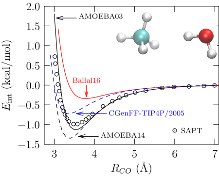
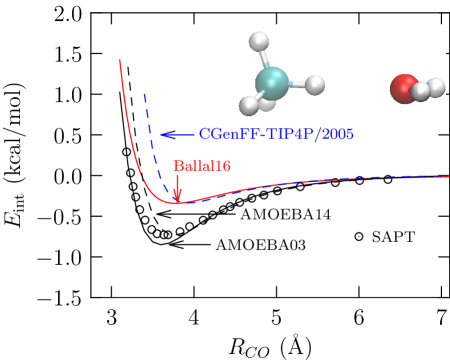
Figure 1: Pair interaction profile between methane and water for the indicated configuration. Top panel: water donates a proton to the electronegative carbon. Bottom panel: oxygen accepts a proton from the methane. AMOEBA03: original AMOEBA water parameters Ren and Ponder (2003); AMOEBA14: AMOEBA water parameters revised to better describe the liquid across a broad temperature range Laury et al. (2015); CGenFF-TIP4P/2005: parameters based on standard Lorentz-Bertholet mixing using the alkane parameter set from CGenFFVanommeslaeghe et al. (2010) and water based on TIP4P/2005Abascal and Vega (2005); Ballal16: parameters noted in Ref. Ballal et al., 2016; methane-water interaction is based on a Lennard-Jones model with energy $\varepsilon_{MeW}=172.05\,k_{\rm B}$ and collision diameter $\sigma_{MeW}=3.365$ Å.

Notice that the AMOEBA03 model captures the location and magnitude of the minima (Fig. 1) quite well. For AMOEBA14 Laury et al. (2015), in the configuration with alkane donating the proton, the minimum is well captured, but the repulsive wall is shifted outwards; and in the configuration with alkane accepting a proton, the minimum is more pronounced. We note that the AMOEBA alkane parameters Ren et al. (2011) were also validated against AMOEBA03 water model, but the hydration free energy of methane in water is better predicted with the AMOEBA14 water model (Appendix VII.1).

The CGenFF-TIP4P/2005 model captures the anisotropy of the interaction, but relative to SAPT neither the location nor the magnitude of the potential minima are well described. The pair-interaction profile based on Ballal et al.’s Ballal et al. (2016) model is able to describe the experimental $\mu^{\rm ex}_{w|a}$ within a united atom framework, but once again neither the location nor the magnitude of the minima are captured. Overall, in comparison with the SAPT results, both the AMOEBA models are significantly better than either CGenFF-TIP4P/2005 or Ballal16 models.

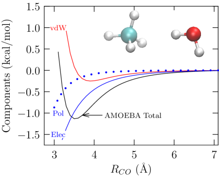
Figure 2: The components of interaction profile according to the AMOEBA interaction model; water is described using the AMOEBA03 paramaters. ‘vdw’: van der Waals interaction; ‘pol’: polarization (or induction) contribution; ‘elec’: electrostatics based on the interacting distributed multipoles.

Dissecting the interaction profile further (Fig. 2), we find that electrostatic interactions, and secondarily induction effects, account for much of the well-depth within the AMOEBA model. Although it is not prudent to infer a particular physical contribution as dominant on the basis of a forcefield description alone, with the background knowledge of the philosophy underlying the AMOEBA forcefield development, the above results collectively suggest that electrostatic interactions and induction effects are important in alkane water interactions.

There is one paradoxical feature in the above results. For the interaction in the specific configurations (Fig. 1), the Ballal16 united atom model clearly does not describe the underlying physics correctly. Yet, this model captures $\beta\mu^{\rm ex}_{w|a}$ quite well. We address this issue next section in the context of the idea of coarse-graining.

IV.2 Solvation of water in n-alkanes

Figure 3 collects $\mu^{\rm ex}_{w|a}$ for all the models considered in this work.

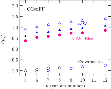
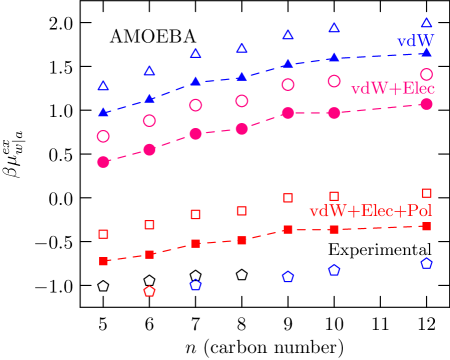
Figure 3: The transfer free energy of water to n-alkanes C_nH_2n+2. Top panel: Results using CGenFF. vdw: only van der Waals interactions considered, and vdW+Elec, both van der Waals and electrostatics interactions included. Bottom panel: Results using AMOEBA03 (open symbols) and AMOEBA14 (corresponding closed symbols with dashed connecting lines to guide the eye) for water. For AMOEBA, vdW+Elec+Pol (polarization) includes all the interactions. Three sets of experimental data are shown using pentagons. Ref. Polak and Lu, 1973, $n=5,6,7,8$; Ref. Roddy and Coleman, 1968, $n=6$; Ref. Schatzberg, 1963, $n=7,9,10,12$. Standard error of the mean for $\beta\mu^{\rm ex}_{w|a}$ is comparable to the size of the symbol and hence is not shown.

Within CGenFF, $\mu^{\rm ex}_{w|a}$ is positive, contrary to experiments. However, the trend with respect to carbon number is correctly captured. Including electrostatic interactions modestly lowers the free energy, emphasizing the role of favorable water-alkane electrostatic interactions in the solvation process.

Both the AMOEBA water models lead to a negative $\mu^{\rm ex}_{w|a}$ and the trend with respect to carbon number is also correctly captured. The average deviation relative to experiments is about 0.25 $k_{\rm B}T$ for AMOEBA14 and 0.5 $k_{\rm B}T$ for AMOEBA03 water models. Within the AMOEBA model, electrostatic interactions play a larger role than in CGenFF, lowering the free energy from the vdW-only value by about 0.5 $k_{\rm B}T$. Interestingly, whereas polarization played a secondary role in the case of a single methane-water pair (Fig. 1), multi-body polarization effects in the condensed phase contribute substantially to lowering the free energy, with the net shift relative to the vdW+Elec case being about 1 $k_{\rm B}T$.

IV.2.1 Coarse graining

As noted above, Ballal et al.’s Ballal et al. (2016) model is able to describe the experimental $\mu^{\rm ex}_{w|a}$ within a united atom framework. In this approach, the SPC/E parameters for water and the TraPPE parameter for alkanes are used, but the Bertholet rule for the effective cross-interaction energy is scaled by a factor 1.6 and the Lorentz rule for the effective collision diameter is scaled by a factor of 0.98. We note that earlier studies show that the results are quite insensitive to small changes in the collision diameter Ballal et al. (2014); Emborsky et al. (2011); Fouad et al. (2014). (In a similar vein, with cross interaction parameters that depart from the Lorentz-Bertholet mixing rule, using the united atom TraPPE model for methane and TIP4P-2005 model for water, Ashbaugh and coworkers Ashbaugh et al. (2010) were able to fit the free energy of hydration of methane in water across a range of temperatures.) We rationalize these results by considering the methane-water pair interaction.

Figure 4 shows the effective pair interaction between methane and water and its various components. This effective pair interaction is obtained by performing an unweighted average over the relative configurations of a methane-water pair for a specified methane (C)-water (O) separation. (The location of the water relative to methane is specified by the spherical angles $\phi$ and $\theta$ and the rotation of the water relative to a fixed frame of reference is specified the Euler angles $\alpha$, $\beta$, and $\gamma$. As usual, we sample $\cos(\theta)$ and $\cos(\beta)$ to avoid singularities and ensure uniform sampling.) Remarkably, the effective methane-water interaction obtained using AMOEBA is close to the Ballal16 united atom model. The effective interaction is dominated by van der Waals, and, to a lesser extent, polarization; the effective electrostatic contribution is nearly zero for all separations. But this should not belie the importance of electrostatics, for without electrostatic interactions, we would not have induction effects (Fig. 2).

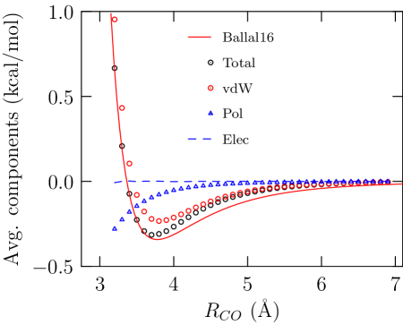
Figure 4: Components of the unweighted angle-average interaction between methane and water using the AMOEBA03 model of water. (The AMOEBA14 model has a slightly lower minima that agrees better with Ballal16.) For each radial separation, on a grid we sample 30 points each for $\phi\in[0,2\pi]$ and for $cos(\theta)\in[-1,1]$. For the orientation of water, with random numbers drawn from a uniform distribution, we choose 30 points from the set $\{\alpha,\cos(\beta),\gamma\}$. In all we sample 9000 configurations for each separation.

The mapping of AMOEBA to the united atom model is an example of coarse graining. It is interesting to consider a similar mapping between AMOEBA and CGenFF. To this end we focus on water solvation in C₅H₁₂. For configurations of n-pentane obtained using AMOEBA, we archive the distribution of electrostatic interaction energies obtained from the test particle procedure. For the same relative orientation of the test water molecule, we also obtain the distribution of electrostatic interaction energy ($\beta\varepsilon_{elec}$) by replacing the AMOEBA distributed multipoles with CGenFF distributed monopoles (i.e. partial charges). For water, we choose the SPC/E partial charge distribution to map the three-site AMOEBA model to another three-site water model. (Using TIP4P/2005 charges will not change the physical conclusion.) Fig. 5 compares the distribution of electrostatic contributions to the interaction energy.

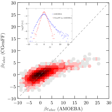
Figure 5: Density plot of the joint distribution $\log P(\beta\varepsilon_{elec}[{\rm AMOEBA}],\beta\varepsilon_{elec}[{\rm CGenFF}])$ of electrostatic interaction energies obtained using AMOEBA and CGenFF. The underlying configurations are the same for both. For CGenFF we use the SPC/E charges for water to preserve the mapping of the 3-site AMOEBA water model to a 3-site fixed charge water model. Every factor-of-$e$ change in the density relative to the mean corresponds to a change in shade. The inset is the projection of the distribution to the respective axis. For clarity, the inset x-axis is cut at $\beta\varepsilon=15$.

Please note that mean interaction energy and the states around the mean are comparably described on the basis of the AMOEBA distributed multipoles and the CGenFF-SPC/E distributed monopoles, but the energy distribution based on the latter model is sharper. Thus as we move away from the mean, the discrepancy in the description of the electrical interaction is higher, with AMOEBA-based electrostatic interaction energies displaying a greater variability. The higher sensitivity of the distributed multipole description is, of course, anticipated. Importantly, in the lower energy wing, AMOEBA-based electrostatics predicts a more negative electrostatic contribution than CGenFF-SPC/E. It is for this reason, that the impact of the electrostatic effects using AMOEBA is higher than that using CGenFF (Fig. 3) .

Returning to the problem of solvation, when we use the united-atom model for computing $\beta\mu^{\rm ex}_{w|a}$, effectively we are taking the average of Boltzmann-factors ($e^{-\beta\Delta U}$) with $\Delta U$ itself an angle-averaged interaction energy, whereas the correct approach would be to use equation Eq. 4 with Boltmann-factors obtained first and then averaged over all configurations. The latter approach of course demands a complete description of the physics. The former approach may work, but it requires the effective interaction model be developed first, perhaps by fitting to available data. Our analysis makes it clear why it should not surprise us if such models lack transferrability. A similar effect undoubtedly underlies the mapping of a fully quantum description of interactions to AMOEBA or AMOEBA to CGenFF, but by preserving more of the physics, these latter coarse-graining steps are likely to allow better transferrability.

With the caveat about forcefields and contributions noted above, our results (Fig. 3) show that electrostatic and induction effects play a decisive role in enhancing the solubility of water in alkanes, but these effects can be masked when we use united-atom models. The success of the AMOEBA model notwithstanding, relative to experiments an admittedly small discrepancy still persists. We consider some possible causes below.

IV.3 Polarization correction and liquid water-to-alkane transfer

The TIP4P-2005 model has an artificially high dipole moment that is required for describing the liquid. Thus it is necessary to correct for this over-polarization in estimating the transfer free energy of TIP4P water from liquid to vapor. However, for transferring the solute from vapor to the apolar alkane phase, one need not apply any corrections and this is partly why we recast the experimental results in terms of vapor to liquid alkane transfer. However, we do make the assumption that the TIP4P-2005 model can be used to describe water-alkane interactions in a water-lean phase. The present study shows that this is unlikely to be satisfactory. A thorough analysis of this issue is left for future studies. We also note that no such polarization issues arise in the AMOEBA model. However, preliminary calculations using quasichemical theory Asthagiri et al. (2003); Weber and Asthagiri (2010) show that the liquid water to vapor transfer free energy using AMOEBA is more positive by about 0.3 kcal/mol than the experimental value for H₂O ($-6.32$ kcal/mol) at 298 K. Thus, if we compared liquid water to alkane transfer free energy, the results with AMOEBA will also be in substantial error.

IV.4 Role of water dimerization

Earlier Ballal et al. (2014) it has been suggested that clustering of water molecules in the alkane phase can potentially contribute to the partitioning of water in the alkane phase. Here we examine this suggestion. First note that as already discussed in Sec. II.1 dimerization in the gas phase proved inconsequential to $\mu^{\rm ex}_{w|v}$. In the alkane phase, to lowest order in solute density the contribution of solute-solute pairing to the excess chemical potential is $2\rho_{w}^{(a)}\tilde{B}_{2}$ Vafaei et al. (2014); Zhang et al. (2014), where $\tilde{B}_{2}$ is the osmotic second virial coefficient. Quantum chemical calculations using B3LYP/6-311+G(d,p) and the SMD continuum solvation model Marenich et al. (2009) shows that association is weaker in the solvent than in the gas-phase at 298 K. (The weakening of interaction in the alkane is analogous to the weakening of association between hydrophobes in water due to solute-water attractive interactions Asthagiri et al. (2008); Ben-Amotz (2015); Chaudhari et al. (2015).) On this basis we can infer that $|\tilde{B}_{2}|<|B_{2}|$ and thus dimerization ought to be inconsequential even in the alkane phase.

IV.5 Role of quantum effects

It is well known that mass effects are important in the phase behavior of water. For example, at 298.15 K the free energy of transferring D₂O from the saturated liquid to the saturated vapor is about 0.14 $k_{\rm B}T$ higher than that for H₂O. Capturing such mass effects at finite temperatures requires treating the motion of nuclei quantum mechanically. (Zero point calculations with the SMD model predict a value of 0.08 $k_{\rm B}T$, qualitatively consistent with the experimental results.) It is clear that the experimental transfer free energy values (Figs. 3) implicitly include the physics of these mass-dependent effects. The AMOEBA03 or AMOEBA14 parameters must also implicitly account for these mass-dependent effects because some of the experimental condensed phase properties are included in the parameter development. However it is unclear whether such a description can apply for transfer across very dissimilar phases. In particular, in transferring a water molecule from the (dilute) vapor phase to the alkane phase, we expect the rotational and vibrational modes of the water molecule to be red-shifted because of interaction with the alkane. Consistent with this intuition, the zero-point energy of a water molecule in the alkane (modeled as a continuous dielectric medium) is lower by $0.1$ $k_{\rm B}T$ relative to that in the vapor. Including this correction over the classical statistical mechanical transfer free energy results (Figs. 3) improves the agreement with experiments. Our analysis of these mass effects is necessarily qualitative; a rigorous treatment of quantum effects associated with nuclear motion Kuharski and Rossky (1985); Guillot and Guissani (1998) could prove rewarding, but such efforts are beyond the scope of this study.

V Concluding Discussion

In discussions of alkane-water interactions, dispersion interactions and, at times the contribution due to the polarizability of the alkane, are most often considered. However, for describing water solubility in alkanes with well benchmarked forcefields such as TraPPE, relying on dispersion interactions alone proves inadequate in capturing the experimentally observed water content in alkanes. The problem arises in modeling water-alkane cross interactions for which conventional mixing rules appear to fail. Thus researchers have had to rely on empirical adjustments for the interactions in the alkane rich and alkane lean phases (for example, see Ref. Bolton et al., 2009). These failures point to missing physics that needs to be accounted in modeling alkane-water interactions.

Our calculations with the AMOEBA all-atom polarizable forcefield is able to describe the experimentally inferred transfer free energy of water from its vapor to a liquid alkane. But even with AMOEBA, relying on van der Waals interactions alone proves inadequate; one must include both electrostatics and induction effects to predict correctly the water content in alkanes. Since the parameters in the AMOEBA forcefield rely extensively on first principles calculations, especially in deriving the atomic polarizability and the distributed multipoles, we conclude that electrostatic interactions and induction effects are important physical ingredients in modeling alkane-water interactions.

We establish the connection between the AMOEBA model and the united atom model with pair-interaction that is empirically adjusted to capture water solubility in alkanes. We show that the unweighted configurationally averaged interaction between methane and water using AMOEBA is in close agreement with the united atom model. The average interaction is dominated by van der Waals and induction effects, the sum of which can be fit to a revised van der Waals potential. But the approximately zero electrostatic contribution should not belie the importance of electrostatics in this interaction. Thus since the united atom models are effective interactions, it is not surprising if we have to re-optimize the interaction between different chemical species in different states of aggregation. Similar comments apply in mapping the physical electrostatic interactions to one described by partial charges alone. Thus using fixed-charge water models such as TIP4P/2005 in a water-lean phase, such as in alkanes or in the interior of biological molecules, may also incur errors, especially if one is interested in the thermodynamics of transfer of the water molecule into such phases. More thoroughly exploring these issues are left for future studies.

VI Acknowledgements

DA, AVP, WGC are grateful for financial support from the Robert A. Welch Foundation (Grant No. C-1241), and the Rice University Consortium for Processes in Porous Media (Houston, TX, USA). DB was supported by the Division of Material Sciences and Engineering, Office of Basic Energy Sciences, U.S. Department of Energy, under Contract No. W-7405-430 ENG-82 with Iowa State University. We thank B. Xue, D. B. Harwood, and J. I. Siepmann for their comments on Ref. Ballal et al., 2014 which led us to correct that work Ballal et al. (2016) and focus on the vapor-to-liquid transfer process. This research used resources of the National Energy Research Scientific Computing Center, a DOE Office of Science User Facility supported by the Office of Science of the U. S. Department of Energy under Contract No. DE-AC02-05CH11231.

VII Appendix

VII.1 Hydration of methane within AMOEBA

To complement the study of water solvation in alkane, we also tested the hydration of methane. To this end, we simulated a box of 512 water molecules and obtained the hydration free energy of methane using Eq. 4. The solvent was simulated at a temperature of 298.15 K and the experimental density of 0.997 gms/cc. The temperature was maintained using an Andersen thermostat. The dispersion interactions were smoothly switched to zero between 9 Å and 10 Å. Electrostatic interactions were treated using Ewald summations with the real-space interaction cut at 10 Å. The time step for integrating the equations of motion was 1 fs.

For either AMOEBA03 or AMOEBA14, we took a pre-equilibrated box of water molecules and equilibrated it further for 250 ps. The subsequent production phase lasted an additional 625 ps. In the production phase configurations were saved every 250 fs to harvest a total of 2500 configurations. The particle insertion calculation was conducted as described in the main text. For methane hydration, for each viable insertion site, we consider five (5) random orientations of the methane molecule. For simplicity we use the single equilibrium geometry of methane, although in the original validation study Ren et al. (2011) the alkane was flexible.

Table 2 collects the results of our studies on methane hydration. We find that the hydration free energy is well estimated using the AMOEBA14 water model, while the AMOEBA03 model underpredicts the hydration free energy by 20%. We must note that in Ref. Ren et al., 2011, the hydration free energy of methane obtained with the AMOEBA03 water model was in near perfect agreement with experiments. The reasons for the discrepancy between our result and the published value is not clear. Perhaps the differences in system size 216 versus 512 water molecules and the assumption of rigid structure of the alkane may explain some of the deviation.

Table 2: Simulated properties of neat water and the hydration free energy of methane on the basis of including only van der Waals ($\mu^{\rm ex}_{v}$), van der Waals plus electrostatics ($\mu^{\rm ex}_{ve}$), and van der Waals, electrostatics, and polarization contributions ($\mu^{\rm ex}_{vep}$). The free energies are in kcal/mol. The experimental hydration free energy is from Ref. Wilhelm et al., 1977.

Property	AMOEBA03	AMOEBA14	Expt.
$\mu^{\rm ex}_{v}$	$2.0\pm 0.03$	$2.5\pm 0.05$	—
$\mu^{\rm ex}_{ve}$	$1.9\pm 0.03$	$2.3\pm 0.05$	—
$\mu^{\rm ex}_{vep}$	$1.6\pm 0.03$	$2.0\pm 0.05$	2.00

The results in Table 2 suggest that electrostatics and polarization also play an important role in the hydration of methane; we expect a similar behavior for other alkanes as well.

References

- Stillinger (1980) F. H. Stillinger, Science 209, 451 (1980).
- Hummer et al. (1998) G. Hummer, S. Garde, A. E. Garcia, M. E. Paulaitis, and L. R. Pratt, J. Phys. Chem. B 102, 10469 (1998).
- Chandler (2005) D. Chandler, Nature 437, 640 (2005).
- Docherty et al. (2006) H. Docherty, A. Galindo, C. Vega, and E. Sanz, J. Chem. Phys. 125, 074510 (2006).
- Ashbaugh et al. (2010) H. S. Ashbaugh, N. J. Collett, H. W. Hatch, and J. A. Staton, J. Chem. Phys. 132, 124504 (2010).
- Akin-Ojo and Szalewicz (2005) O. Akin-Ojo and K. Szalewicz, J. Chem. Phys. 123, 134311 (2005).
- Ballal et al. (2014) D. Ballal, P. Venkataraman, W. A. Fouad, K. R. Cox, and W. G. Chapman, J. Chem. Phys. 141, 064905 (2014).
- Ballal et al. (2016) D. Ballal, D. Asthagiri, A. V. Parambathu, P. Venkataraman, W. A. Fouad, K. R. Cox, and W. G. Chapman, J. Chem. Phys. 145, 119901 (2016).
- Martin and Siepmann (1998) M. Martin and J. I. Siepmann, J. Phys. Chem. B 102, 2569 (1998).
- Berendsen et al. (1987) H. J. C. Berendsen, J. R. Grigera, and T. P. Straatsma, J. Phys. Chem. 91, 6269 (1987).
- McDaniel and Yethiraj (2016) J. G. McDaniel and A. Yethiraj, J. Chem. Phys. 144, 137101 (2016).
- Jiang et al. (2017) H. Jiang, I. G. Economou, and A. Z. Panagiotopoulos, J. Phys. Chem. B 121, 1386 (2017).
- Ren and Ponder (2003) P. Ren and J. W. Ponder, J. Phys. Chem. B 107, 5933 (2003).
- Laury et al. (2015) M. L. Laury, L.-P. Wang, V. S. Pande, T. Head-Gordon, and J. W. Ponder, J. Phys. Chem. B 119, 9423 (2015).
- Ren et al. (2011) P. Ren, C. Wu, and J. W. Ponder, J. Chem. Theory Comput. 7, 3143 (2011).
- Stone (2013) A. J. Stone, The theory of intermolecular forces (Oxford University Press, Oxford, UK, 2013), 2nd ed.
- Polak and Lu (1973) J. Polak and B. C.-Y. Lu, Canadian J. Chem. 51, 4018 (1973).
- Roddy and Coleman (1968) J. W. Roddy and C. F. Coleman, Talanta 15, 1281 (1968).
- Schatzberg (1963) P. Schatzberg, J. Phys. Chem. 67, 776 (1963).
- Lemmon et al. (2017) E. W. Lemmon, M. O. McLinden, and D. G. Friend, NIST chemistry webbook, NIST standard reference database number 69 (National Institute of Standards and Technology, Gaithersburg, MD, 2017), chap. Thermophysical properties of fluid systems.
- Harvey and Lemmon (2004) A. H. Harvey and E. W. Lemmon, J. Phys. Chem. Ref. Data 33, 369 (2004).
- Widom (1982) B. Widom, J. Phys. Chem. 86, 869 (1982).
- Paulaitis and Pratt (2002) M. E. Paulaitis and L. R. Pratt, Adv. Phys. Chem. 62, 283 (2002).
- Beck et al. (2006) T. L. Beck, M. E. Paulaitis, and L. R. Pratt, The Potential Distribution Theorem And Models Of Molecular Solutions (Cambridge University Press, Cambridge, UK, 2006).
- Pratt and Asthagiri (2007) L. R. Pratt and D. Asthagiri, in Free Energy Calculations: Theory And Applications In Chemistry And Biology, edited by C. Chipot and A. Pohorille (Springer, Berlin, DE, 2007), vol. 86 of Springer series in Chemical Physics, chap. 9, pp. 323–351.
- Abascal and Vega (2005) J. L. F. Abascal and C. Vega, J. Chem. Phys. 123, 234505 (2005).
- Vanommeslaeghe et al. (2010) K. Vanommeslaeghe, E. Hatcher, C. Acharya, S. Kundu, S. Zhong, J. Shim, E. Darian, O. Guvench, P. Lopes, I. Vorobyov, et al., J. Comp. Chem. 31, 671 (2010).
- Hanwell et al. (2012) M. D. Hanwell, D. E. Curtis, D. C. Lonie, T. Vandermeersch, E. Zurek, and G. R. Hutchinson, J. Comp. Chem. 4, 17 (2012).
- Martinez et al. (2009) L. Martinez, R. Andrade, E. G. Birgin, and J. M. Martinez, J. Comp. Chem. 30, 2157 (2009).
- Phillips et al. (2005) J. C. Phillips, R. Braun, W. Wang, E. Tajkhorshid, E. Villa, C. Chipot, R. D. Skeel, L. Kale, and K. Schulten, J. Comp. Chem. 26, 1781 (2005).
- Ponder (2015) J. W. Ponder, TINKER molecular modeling package V7.1, Washington University Medical School, St. Louis, MO (2015).
- Asthagiri et al. (2008) D. Asthagiri, S. Merchant, and L. R. Pratt, J. Chem. Phys. 128, 244512 (2008).
- Hummer et al. (1992) G. Hummer, D. M. Soumpasis, and M. Neumann, Mol Phys 77, 769 (1992).
- Hummer and Soumpasis (1994) G. Hummer and D. M. Soumpasis, Phys. Rev. E 49, 591 (1994).
- Hummer et al. (1994) G. Hummer, D. M. Soumpasis, and M. Neumann, J. Phys.: Cond. Mat. 6, A141 (1994).
- Allen and Tildesley (1987) M. P. Allen and D. J. Tildesley, Computer simulation of liquids (Oxford University Press, 1987), chap. 6. How to analyze the results, pp. 192–195.
- Friedberg and Cameron (1970) R. Friedberg and J. E. Cameron, J. Chem. Phys. 52, 6049 (1970).
- (38) M. J. Frisch, G. W. Trucks, H. B. Schlegel, G. E. Scuseria, M. A. Robb, J. R. Cheeseman, G. Scalmani, V. Barone, B. Mennucci, G. A. Petersson, et al., Gaussian∼09 Revision E.01, gaussian Inc. Wallingford CT 2009.
- Emborsky et al. (2011) C. P. Emborsky, K. R. Cox, and W. G. Chapman, Ind. Eng. Chem. Res. 50, 7791 (2011).
- Fouad et al. (2014) W. A. Fouad, D. Ballal, K. R. Cox, and W. G. Chapman, J. Chem. Eng. Data 59, 1016 (2014).
- Asthagiri et al. (2003) D. Asthagiri, L. R. Pratt, and J. D. Kress, Phys. Rev. E 68, 041505 (2003).
- Weber and Asthagiri (2010) V. Weber and D. Asthagiri, J. Chem. Phys. 133, 141101 (2010).
- Vafaei et al. (2014) S. Vafaei, B. Tomberli, and C. G. Gray, J. Chem. Phys. 141, 154501 (2014).
- Zhang et al. (2014) W. Zhang, X. You, and L. R. Pratt, J. Phys. Chem. B 118, 7730 (2014).
- Marenich et al. (2009) A. V. Marenich, C. J. Cramer, and D. G. Truhlar, J. Phys. Chem. B 113, 6378 (2009).
- Ben-Amotz (2015) D. Ben-Amotz, J. Phys. Chem. Lett. 6, 1696 (2015).
- Chaudhari et al. (2015) M. I. Chaudhari, S. B. Rempe, D. Asthagiri, L. Tan, and L. R. Pratt, J. Phys. Chem. B 120, 1864 (2015).
- Kuharski and Rossky (1985) R. A. Kuharski and P. J. Rossky, J. Chem. Phys. 82, 5164 (1985).
- Guillot and Guissani (1998) B. Guillot and Y. Guissani, J. Chem. Phys. 108, 10162 (1998).
- Bolton et al. (2009) K. Bolton, E. Johansson, L. Jönsson, and P. P. Ahlström, Molec. Sim. 35, 888 (2009).
- Wilhelm et al. (1977) E. Wilhelm, R. Battino, and R. J. Wilcox, Chem. Rev. 77, 219 (1977).