Cosmological discordances: A new measure, marginalization effects, and application to geometry versus growth current data sets
Abstract
The continuous progress toward more precise cosmological surveys and experiments has galvanized recent interest into consistency tests on cosmological parameters and models. At the heart of this effort is quantifying the degree of inconsistency between two or more cosmological data sets. We introduce an intuitive moment-based measure we call the index of inconsistency (IOI) and show that it is sensitive to the separation of the means, the size of the constraint ellipsoids, and their orientations in the parameter space. We find that it tracks accurately the inconsistencies when present. Next, we show that parameter marginalization can cause a loss of information on the inconsistency between two experiments and we quantify such a loss using the drop in IOI. In order to zoom on a given parameter, we define the relative residual IOI and the relative drop in IOI. While these two quantities can provide insights on the parameters that are most responsible for inconsistencies, we find that the full IOI applied to the whole parameter spaces is what must be used to correctly reflect the degree of inconsistency between two experiments. We discuss various properties of IOI, provide its eigenmode decomposition, and compare it to other measures of discordance. Finally, we apply IOI to current geometry data sets (i.e. an improved Supernovae Type Ia compilation, baryon acoustic oscillations from 6dF, SDSS MGS and Lyman- forest, and high- cosmic microwave background (CMB) temperature data from Planck-2015) versus growth data sets (i.e. Redshift Space Distortions from WiggleZ and SDSS, Weak Lensing from CFHTLenS, CMB Lensing, Sunyav-Zeldovich effect, and low- CMB temperature and polarization data from Planck-2015). We find that a persistent inconsistency is present between the two data sets. This could reflect the presence of systematics in the data or inconsistencies in the underlying model.
pacs:
98.80.Es,95.36.+x,98.80.-kI Introduction
The CDM standard model of cosmology enjoys a number of observational confirmations and successes. However, it does come with two intriguing conundrums. The first one is that it requires a dark matter component counting for about of matter-energy content in the Universe. The second one is that the expansion of the Universe is accelerating and we do not know what is driving this acceleration. Associated with this cosmic acceleration is a dark energy component that could count for about of the energy budget in the Universe. These and other questions have motivated studies to consider if there are any problems with the underlying model, theory or assumptions. See, for example, Refs. Clifton et al. (2012); López-Corredoira (2017); Tsagas et al. (2008); Koyama (2016); Joyce et al. (2015); Ishak (2007); Joyce et al. (2016); Bull et al. (2016); Debono and Smoot (2016) and references therein.
One route to test this that is attracting more attention lately is to compare results and parameters from different experiments and then to look for any inconsistencies. Over a decade ago, Ref. Ishak et al. (2006) used simulated data sets to demonstrate how inconsistencies between the dark energy parameter spaces as constrained by the expansion versus the growth can signal a failure of the underlying gravity theory. A related method called “parameter splitting” was applied to real data in Refs. Wang et al. (2007); Ruiz and Huterer (2015); Bernal et al. (2016a) and looked for inconsistencies between dark energy parameters as constrained by expansion versus the growth. References. Shafieloo (2012); Shafieloo and Hazra (2017) introduced a technique called the crossing function, which enables us to see if the best fit from one experiment is consistent with the constraints from another experiment.
Most recently, a number of papers have focused on possible discrepancies between cosmological parameters as constrained by different experiments. While some have faded away, some others seem to persist; see, for example Refs. Bernal et al. (2016b); Di Valentino et al. (2015); Aubourg et al. (2015); Heymans et al. (2013); Charnock et al. (2017). We take the point of view that whether due to systematic effects in the data or due to underlying physics, these discrepancies need a careful study. Otherwise, a joint analysis will be of questionable outcome. In the next section, we review briefly some of the inconsistencies or tensions that have appeared in the literature.
An important question is to quantify the degree of inconsistency or tension. Very often, the inconsistency between two experiments is qualitatively shown in marginalized one-dimensional (1D) or two-dimensional (2D) likelihood contour plots. However, as we demonstrate in this paper, this method cannot accurately represent the inconsistency. First of all, it is not a quantitative method, rendering it difficult to be interpreted in an accurate way. Secondly, if the underlying model has three or more parameters this method fails to account for the full inconsistency. Moreover, as shown later in this work, listing all the marginalized 1D or 2D plots does not properly represent the full inconsistency either. Therefore some measures have been introduced in the literature in order to quantify inconsistencies between two experiments, and we review most of them in Sec. X. An important criterion is that a measure must properly describe experimental discordances.
In this paper, we define and apply a measure of inconsistency that is found to track accurately inconsistencies. It is a moment-based quantity that we call the index of inconsistency (IOI). This can be applied to two or more experiments or data sets. We find that in the Gaussian and weak prior limit, most other measures in the literature reduce to or contain a term of IOI. This measure properly describes the factors causing the inconsistency: i.e mean difference, constraint volumes and their orientations.
Importantly, we also show here that parameter marginalization can hide inconsistency. We argue that a good measure of inconsistency should reflect this. When zooming on specific parameters, we define the relative drop in IOI and the relative residual IOI. This allows one to track down the inconsistencies and find parameters that are most subject to these inconsistencies.
Finally, we apply the new measures and study the inconsistency between the geometry data sets and the growth data sets. For the geometry, we use the type Ia supernovae compilation in Ref. Betoule et al. (2014), the baryon acoustic oscillation (BAO) from the Six Degree Field Galactic Survey (6dF) Beutler et al. (2011), the main galaxy sample from the Sloan Digital Sky Survey (SDSS-DR7) and the SDSS quasar-Lyman- forest Aubourg et al. (2015), and the high- CMB temperature data from Planck 2015 Ade et al. (2016a) (Planck Collaboration). For the growth, we use the low- CMB temperature and polarization data form Planck 2015 Ade et al. (2016b) (Planck Collaboration), CMB lensing Ade et al. (2016b) (Planck Collaboration), thermal Sunyaev–Zel’dovich effect Ade and others (2016) (Planck Collaboration), cosmic shear from the Canada France Hawaii Lensing Survey (CFHTlens) Heymans et al. (2013), and the redshift space distortion (RSD) from the WiggleZ Dark Energy Survey (WiggleZ MPK) Blake et al. (2010); Parkinson et al. (2012) and the SDSS DR12 CMASS and LOWZ catalogs Alam et al. (2015). This application is motivated by the fact that modified gravity theory can lead to inconsistency on the dark energy properties when fitting CDM or CDM model separately into the geometry and the growth sets of experiments, and also in order to quantify the degree of inconsistency between these two data sets as reported in some previous works.
We organize our paper as follows: In Sec. II we review some inconsistencies among different cosmological experiments. In Sec. III we define IOI, demonstrate that it can properly describe the inconsistency between two experiments, discuss its properties, and show that it correctly reflects the effects of marginalization. In Sec. X we view other measures of experimental inconsistency in the literature, and point out some limitations. Then in Sec. XI we apply IOI along with some other measures in Gaussian and weak prior limit to the geometry and the growth experiments based on the CDM and the CDM models. Finally we summarize our work in Sec. XII. In this work, “inconsistency”, “tension” and “discordance” share the same meaning, but the quantities IOI, the tension (), and the discordance are different measures of inconsistency.
II Brief survey of reported tensions or inconsistencies
In this section we list some inconsistencies or tensions between cosmological experiments as reported in the literature. Again, regardless if these are caused by different systematic effects in various data sets or caused by shortcomings in the cosmological model, they require careful examination.
Hubble constant tension: A precise locally measured Hubble constant by ladder distance observation is given as by Refs. Riess et al. (2016, 2011), which is higher than the one derived from the Planck 2015 data assuming the CDM model Adam and others (2016a) (Planck Collaboration). The tension is reported as at a 3.4- confidence level in Ref. Riess et al. (2011). Reference Bernal et al. (2016b) used their measure called the tension and reported a high inconsistency between the local measurement of and the Planck result. They found that the odds for the two experiments to be consistent one with another are only .
In order to locally measure the Hubble constant, one needs to hierarchically calibrate the distances to different celestial objects, so papers have pointed out the systematic effects involved. For example, Ref. Efstathiou (2014) adopted a different outlier rejection criteria in the Cepheid samples and find that the high value of the locally measured Hubble constant in Ref. Riess et al. (2011) could be due to a systematic error in the distance calibration. But recently authors in Ref. Riess et al. (2016), using more Cepheid variables calibrated type Ia supernova, confirmed their earlier high value found in Ref. Riess et al. (2011). Also Ref. Casertano et al. (2017) using Gaia Data Release 1 reported a similarly high value of the Hubble constant (), different from the Planck measurement at - level. So the tension of between local measurements and the Planck 2015 result still remains. The authors of Ref Bonvin et al. (2017) independently measured the Hubble constant based on time delay strong lensing, and reported in the CDM model consistent with the local measurement.
On the other hand, this tension might indicate a possible problem with the underlying model. For example, if the CDM model is extended to the CDM model, it was claimed in Ref. Huang and Wang (2016) that a piecewise function of can reconcile the derived Hubble constant from the Planck data with the one locally measured. Reference Di Valentino et al. (2016a) showed that varying 12 cosmological parameters can solve the current tension on between Planck and local measurement. But they also pointed out that tension remains if BAO and distances to supernova are included in the joint analysis.
Gravitational Lensing and Planck: Another persisting tension is between cosmic shear experiments and Planck for the determination of the amplitude of matter density fluctuations as, for example, parametrized by . CFHTlenS Heymans et al. (2013) found a lower amplitude than Planck 2015 Ade et al. (2016a) (Planck Collaboration). In the marginalized vs plane, the CFHTlenS confidence contours are shifted to the upper left compared to the Planck 2015 results. Most recently, the KIDS-450 survey finds a similar discrepancy at a 2.5- level for Hildebrandt et al. (2017) and claims a substantial discordance in the full parameter space compared to Planck 2015. Finally, the authors of Ref. Leauthaud et al. (2017) used galaxy-galaxy lensing measurements of the BOSS CMASS sample using 250 square degrees of weak lensing from CFHTLenS and CS82 and found also a lower value of than that of Planck 2015. They pointed out that this can be caused by systematics or new physics. Indeed, a number of systematic effects for lensing require more work such as intrinsic alignment of galaxies, baryonic effects, and photometric redshifts Troxel and Ishak (2015); Kirk et al. (2015); Eifler et al. (2015); Dossett et al. (2015); Krause et al. (2016). On the other hand, it was pointed out in Refs. Di Valentino et al. (2015, 2016a) that the tension between CFHTlenS and Planck can be solved by varying (lensing anomaly parameter).
BAO at z=2.34: The baryon acoustic oscillation in the Lyman- forest measurement gives the ratio of the Hubble radius to the drag epoch sound horizon at Aubourg et al. (2015), which combines the Ly forest autocorrelation Delubac et al. (2015) and the quasar-Ly cross-correlation Font-Ribera et al. (2014) methods. If we take Mpc-1 form Planck 2015 Ade et al. (2016a) (Planck Collaboration), the inferred Hubble parameter at is 111Since .. On the other hand, the Planck 2015 best fit gives , which is higher than the one derived from BAO Lyman- forest measurement. It is suggested that this discrepancy could be evidence for the interacting dark energy and dark matter model, see, for example Ferreira et al. (2017).
CMB Lensing anomaly: The CDM model predicts a certain strength of the CMB lensing potential. In Ref. Calabrese et al. (2008) a lensing anomaly parameter defined as was introduced (where and are the observed and predicted lensing-potential power spectra) to test such an amplitude. If CDM is a consistent model on the CMB temperature, polarization and lensing observation, this lensing anomaly parameter must be unity, . Early the WMAP (along with ACBAR) data give at the confidence level Calabrese et al. (2008), meaning the observed lensing potential is significantly higher than expected. However, this high value of did not persist in the Planck data, and dropped to at the confidence level Ade et al. (2016a) (Planck Collaboration). So although there is still a small gap between and unity, it became more consistent with the prediction of the CDM model. Nevertheless, it was shown that modified-gravity equations for the two scalar potentials (in the Newtonian gauge) can solve this small lensing anomaly Di Valentino et al. (2016b). They claimed that this lensing anomaly gives a preference for modified gravity at a confidence level. The authors in Ref. Muñoz et al. (2016) found that adding compensated isocurvature perturbations to the CDM model can solve such a CMB lensing anomaly.
Redshift Space Distortion (RSD) and Cluster Abundance vs Planck: Compared to what is inferred from Planck 2015 best fit, RSD measurements generally give smaller growth of the large structure parametrized as , where is the growth rate; see for examples Refs. Blake et al. (2011); Bernal et al. (2016a); Reid et al. (2014). The two most precise galaxy cluster abundance measurements also seem to have significant tensions with the Planck 2015 results in the marginalized - plane. One is the x-ray as a mass tracerfrom the Chandra cluster cosmology project Vikhlinin et al. (2009), and the other is the thermal Sunyaev-Zel’dovich effect from Planck itself Ade and others (2016) (Planck Collaboration); also see Ref. Bernal et al. (2016a).
Geometry versus Growth: When combined, geometry probes and growth probes provide powerful combinations to constrain cosmology. Moreover, when one is contrasted with another they constitute a useful consistency test of the underlying theory Ishak et al. (2006); Koyama (2006); Bertschinger (2006) or a mean to detect different systematics in the data sets. The authors of Refs. Wang et al. (2007); Ruiz and Huterer (2015); Bernal et al. (2016a) used a technique called parameter splitting, in which they separate parameters constraining the dark energy properties (e.g., and ) into a geometry set (e.g., and ) and a growth set (e.g., and ). Authors of Ref. Ruiz and Huterer (2015) found that RSD data generally favor a higher , and Ref. Bernal et al. (2016a) found that a subset of cluster abundance data (from Refs. Vikhlinin et al. (2009); Ade and others (2016) (Planck Collaboration)) mostly cause the deviations of dark-energy metaparameters.
III Index of inconsistency: motivation and definition
Different works on measures of inconsistency in the literature adapt different notations. For a consistent discussion throughout the paper, we use the following notation so Bayes’s theorem reads
| (1) |
where is the posterior probability distribution, the likelihood, the prior and the evidence. Most of the experiments discussed here are assumed to give Gaussian likelihoods on the parameters. For Gaussian likelihoods,
| (2) |
where is the parameter vector, the mean ( for two experiments), and the Fisher matrix. For mildly non-Gaussian distributions, the above equation is treated as an approximation to the real distribution, with and given by the mean and inverse of the covariance matrix of the real distribution. The mean is a function of the data vector . Experiments are assumed to have the same Gaussian prior distribution
| (3) |
where and is the inverse of the covariance matrix of the prior. A weak prior limit is taken as . The Gaussian and weak prior limit refers to a situation where likelihoods are Gaussian on the parameters and the prior is weak. Posteriors are normalized, and are denoted as . The inverse of the covariance matrix of a posterior is denoted as , and the mean as . Some common notations in this work are summarized in Tables 2 and 2.
| Distributions | Notations |
Inverse of
covariance matrix |
Elements of
Fisher matrices |
Means |
Elements
of means |
|---|---|---|---|---|---|
| th Likelihood | |||||
| Prior | |||||
| th Posterior |
| Parameter vector | Observable vector | Mean difference | Covariance matrix | matrix |
|---|---|---|---|---|
III.1 Motivation for IOI
In the Bayesian parameter estimation, experiments give probability density distributions of the parameters in a given model. Different experiments usually give different distributions. The joint distribution is the one obtained by simultaneously analyzing the data from two or more experiments. Figure 1 shows two toy 1D Gaussian distributions (red and blue) given by two different experiments, and their joint distribution (black dotted) on parameter .
We can see in Fig. 1 that the red distribution favors the value of at , while the blue one favors at , so there is an inconsistency between the two experiments. One might want to use the difference of the two means to quantify the inconsistency, i.e., . But this method cannot be right, because the mean difference is not invariant under a parameter scaling. If we let , the new means become and , and the difference becomes . The inconsistency between two experiments for a model should not depend on the scaling.
One then realizes that the mean difference needs to be normalized by the uncertainties of the distributions, since the uncertainties will be scaled inversely as the mean difference. And this normalization makes perfect sense: if the uncertainties are very large compared to the mean difference, the inconsistency will actually be small. But which distribution’s uncertainty should be used to normalize the mean difference? Intuition tells us that we should not use just one but somehow both of them. One might want to use the uncertainty of the joint distribution. For example, the figure of bias (Fob) defined in Ref. Shapiro (2009) reduces to this type of form in one dimension. But this choice has problems for the reasons that follow. Suppose the uncertainties of the red and the blue distributions are and ; the uncertainty of the joint distribution is given by . Normalizing by will give a quantity such as . If one distribution has a much smaller uncertainty than the other, say , that quantity can be approximated as . So in this situation the mean difference is normalized only by , and it diverges as . This is very counterintuitive. If one uncertainty is very small but the other is very large, the inconsistency should be small. That is because the distribution with a large uncertainty can extend to the mean of the other distribution that has a small uncertainty. So if , the mean difference should be normalized by instead of . Therefore, instead of , it is a quantity such as that should be used.
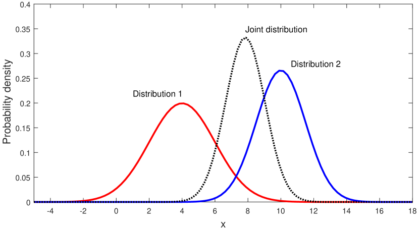
Here, we approach the inconsistency in a slightly different way from above. Indeed, the above discussion did not consider the mean of the joint distribution. Instead of using the difference between the means of the two distributions, we use two differences. One difference is between the first distribution mean and the joint distribution mean, and the other difference is between the second distribution mean and the joint distribution mean. Then we normalize the first difference by the first uncertainty, and the second difference by the second uncertainty. Finally we take the average of the normalized mean differences (squared) as the measure of inconsistency. More precisely, we use the following quantity to measure the inconsistency,
| (4) |
The meaning of Eq. (4) is as follows: it is the average of two terms, each of which measures the “difficulty” for the corresponding distribution to “support” or “favor” the mean of the joint distribution. The mean of the joint distribution will be closer to the mean of the distribution with a smaller uncertainty. For a metaphor, if two people are separated, one is at location A and the other is at location B. We can use the minimum time taken by them to meet to quantify the degree of how they are separated. Surely both of them need to move, and the one who travels faster or moves easier needs to make a longer distance.
We will show in Sec. III.2 that the above quantity actually turns out to be
| (5) |
which has the same form as the one we logically obtained in the previous paragraph.
So far we have only considered 1D distributions, but let us “extrapolate” the result to multidimensional distributions. For multidimensional Gaussian distributions, the uncertainty (squared) is specified by the covariance matrix . So, it is reasonable to guess the general form of Eq. (5) to be , and it turns out to be a proper guess as we demonstrate in Sec. III.2.
III.2 Definition of IOI
We first define the term as
| (6) |
with . We can see that between two experiments is defined as an average of two terms, namely,
-
The difficulty for the first experiment to support the mean of the joint analysis.
-
The difficulty for the second experiment to support the mean of the joint analysis.
So is the averaged difficulty for the two experiments to support the joint mean. This definition of is equivalent to , where and “min” means minimum of (and maximum of likelihood).
As shown in Appendices A.1 and A.2, in the Gaussian limit where , the mean of the joint likelihood is given by a Fisher-matrix-weighted average,
| (7) |
where . And then , in this limit, can be computed explicitly as
| (8) |
Thus, we define IOI for two experiments to be the Gaussian limit of [Eq. (6)] and given by
| (9) |
where , and . This result is the same as our guided guess in Sec. III.1. In the cases of Gaussian likelihoods, IOI is the same as . But in general cases, we define IOI as the moment-based quadratic quantity , with obtained by the inverse of the covariance matrices and given by the means. So the definition of IOI is only motivated by , but not itself. IOI is a moment-based quadratic quantity.
| Ranges | IOI | IOI | IOI | IOI |
|---|---|---|---|---|
| Interpretation |
No significant
inconsistency |
Weak
inconsistency |
Moderate inconsistency |
Strong
inconsistency |
If we have priors assigned to the two experiments, we can extend the definition of IOI to include priors in the means and covariance matrices as follows:
| (10) |
where for Gaussian distributions and is an approximation in mildly non-Gaussian cases. Thus Eq. (9) is the weak prior limit () of Eq. (10). However, we suggest to use Eq. (9) to compare two experiments for the following reasons. First, we usually have only weak priors on parameters. Second, the priors might already be biased or in tension with the experiments considered. Two experiments should be compared with very weak priors. Including strong priors may affect the comparison of two experiments. But, of course, we can use Eq. (9) to compare and see if the prior is consistent with the experiments to be compared, by simply replacing and with and in Eq. (9).
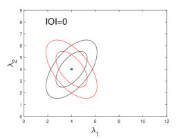
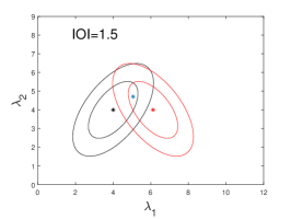
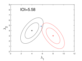
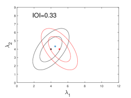
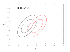
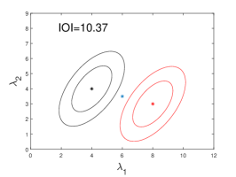
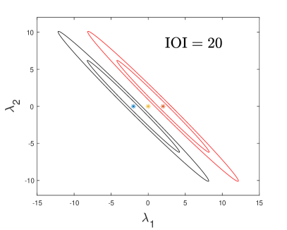
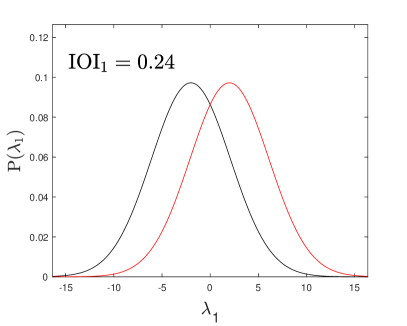
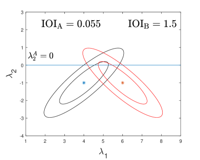
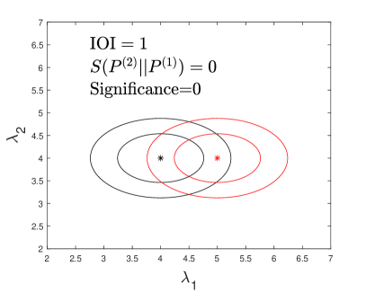
For illustration, we show in Fig. 2 some examples of toy likelihood contours with their corresponding values of IOI. Those examples show that IOI can properly represent inconsistency between two experiments; i.e., it increases whenever the experimental inconsistency increases graphically. We use Jeffreys’ scale (shown in Table 3; see Ref. Jeffreys (1998)) as an interpretation of the values of IOI. Note that Jeffreys’ scales were originally empirical scales for the Bayesian evidence ratio. Here IOI is not an evidence ratio but we use this empirical scale as it seems to give sensible meanings for the inconsistencies compared to what is shown in Fig. 2. Moreover, reference Verde et al. (2013) proposed a quantity called tension to measure experimental inconsistency. They used Jeffreys’ scale as the interpretation of the tension. We will show further in the paper that the tension reduces to IOI in the Gaussian and weak prior limit. So we expect that IOI and the tension are similar quantities for nearly Gaussian distributions, and using the same scale is good for comparison. However, we note again that one should not translate IOI into a probability ratio, although we propose Jeffreys’ scales as the interpretation of IOI.
The next logical step is to generalize Eq. (9) to define IOI for comparison of experiments as
| (11) |
| (12) |
where is the mean of the joint likelihood combining all experiments and it is also given by the Fisher-matrix-weighted average,
| (13) |
where . Each term in the sum in the left-hand side of Eq. (11) has the same interpretation as that in Eq. (6), which is measuring the difficulty for the th experiment to support the mean of the joint analysis. So represents the averaged difficulty for the experiments to support their joint mean. We have again taken the Gaussian limit of Eq. (11) and defined IOI for experimental as the moment-based quantity Eq. (12). But since Eq. (12) contains more than two means, it cannot be reduced into a quadratic form as in the case of two experiments. For the case of two experiments, the two different forms Eq. (9) and Eq. (12) are equivalent; see Appendix A.2.
Before closing this subsection, we give some remarks. Our IOI and other measures of inconsistency in the literature are a model-dependent description of inconsistency between experiments. For example, in Sec. XI we will see that IOI between the geometry experiments growth experiments for the CDM model is different from that for the CDM model. Reference Verde et al. (2013) suggested that a better model should provide more consistent explanations on different experiments. With IOI, it means a better model should give a smaller IOI on two or more experiments.
III.3 Inconsistency measures and Gaussianity
Current cosmological experiments usually provide approximately Gaussian probability distributions on parameters. In those cases, it is usual to approximate the actual probability distribution by a Gaussian one based on its moments. The mean and covariance matrix of the approximate Gaussian distribution are taken to be those of the actual distribution. If a measure does not correctly describe inconsistency in Gaussian cases, one would not expect it to correctly describe inconsistency in general. Therefore constructing a correct measure of inconsistency for Gaussian and nearly Gaussian cases is an important step to the measure for general cases, and this is what we aim to accomplish in this work. We argue that IOI works correctly in Gaussian cases, and we expect it to give meaningful information in mildly non-Gaussian cases. So IOI has an important role: one can compare a measure with IOI to see whether that measure properly describes experimental inconsistency in Gaussian cases.
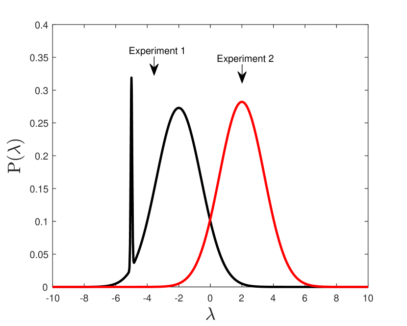
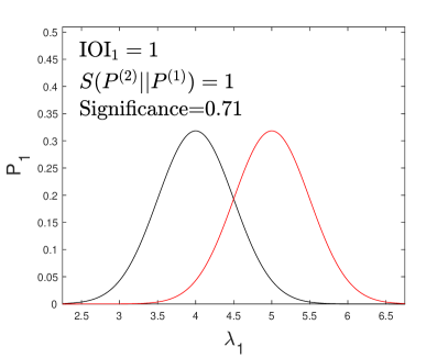
However, we do not expect IOI to describe inconsistency properly in highly non-Gaussian cases. In fact, it is even difficult to define inconsistency when distributions are non-Gaussian. There might be other criteria to consider for general cases, which need to be further explored in future works. We note that even if a measure reduces to IOI in the Gaussian limit, it does not necessarily mean such a measure can describe inconsistency properly. For example, in the Gaussian limit is the same as IOI, but it can give us misleading results in some non-Gaussian cases as we will explain. focuses on its minimum value but ignores the overall distribution. For example, in Fig. 3 the 1D probability distribution given by experiment 2 is Gaussian, while given by experiment 1 is not. In fact, is only slightly different from a Gaussian distribution: there is a narrow local peak at which is also the global maximum of ; the rest of is overall Gaussian. When we compare the two experiments, intuition tells us we can ignore that narrow peak. That is because the integrated probability around that peak is small compared to the rest, which gives it a negligible probability weight. So even for such a mildly non-Gaussian distribution, does not work. One would expect the situation shown in Fig. 3 can be approximated by two Gaussian distributions. That is exactly what the moment-based IOI does. Compared to the case without the narrow peak, with that peak only slightly changes the parameters’ means and covariance and the value of IOI.
It is worth noting that IOI is invariant under a linear parameter transformation, with a transformation matrix . Under such a transformation, the mean difference becomes and the Fisher matrices become . Then IOI transforms as
| (14) |
However, IOI is not invariant under a general invertible parameter transformation which should be a desirable property for a measure of inconsistency. IOI is only nearly invariant under an invertible parameter transformation that can be approximated by a linear transformation in the parameter region of interest. The parameter region of interest here means the parameter space spanned by several confidence levels around the joint mean. Constructing a measure based on IOI, which can describe inconsistency for general cases and is general parameter invariant, is out of the scope of this paper and is left for future work.
IV Factors affecting IOI and inconsistency measures
Experimental inconsistencies are affected by at least three factors: the likelihood mean deviation, the volume of the covariance matrix (how big the iso-likelihood ellipses are), and the degeneracy directions (orientations of the ellipses). The first two factors are related in an obvious way to degree of inconsistency. Basically a larger mean deviation and a smaller covariance matrix volume give a larger experimental inconsistency. The third factor is a little bit more subtle and can be seen as follows. Let us consider the two right panels in Fig. 2 for example. We can see that those two panels have the same mean deviation and the same covariance matrix volumes, but the upper obviously has a smaller inconsistency due to different constraint orientations. So how does IOI relate to and describe different constraint orientations? We recall that IOI incorporates the joint mean to specify the inconsistency. For a given mean deviation and constraint volumes, the orientations of those ellipses determine the location of the joint mean. If the ellipse orientations make the joint mean to locate closer to the mean of each experiment mean, then IOI will be smaller, and vice versa. A different set of ellipse orientations leads to a different matrix and a different IOI. So for the case of two experiments, the third factor of inconsistency is reflected by the matrix . The values of IOI can then describe such a change of the graphical inconsistency due to the change of ellipse orientations.
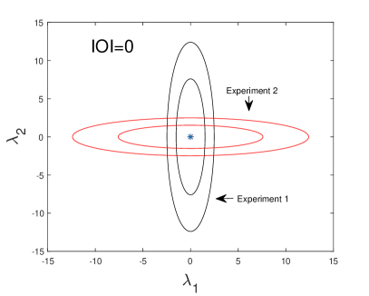
We discussed how the lower right panel in Fig. 2 has a larger inconsistency than the upper right panel and explained that this is because the ellipse orientations in the lower panel make the joint mean further away from each individual mean. However, it is not correct to associate the larger inconsistency in the lower panel with the smaller “overlap” between the two ellipses compared to the upper panel. A smaller overlap does not necessarily mean a larger inconsistency, as we will explain. We recall that the purpose of a (in)consistency check is to see whether we can jointly study two or more experiments. Two experiments can have a small overlap but still be consistent with each other. Take Fig. 4 for example. The two toy experiments have orthogonal degenerate directions, which give them a small overlap. The small overlap here does not prevent us from jointly studying the two experiments, so we say the two experiments are consistent with each other. Thus, this kind of small overlap should not be counted as an increase of inconsistency. Some might worry that the small overlap here means the two distributions are different. But a (in)consistency test is not to look for difference between experiments, but to see if they share anything in common. To see this again, let us assume for a moment that the small overlap does suggest an increase of inconsistency. Imagine that we have a third experiment with a diagonal () degenerate direction going through the overlap of the previous two experiments. Now the three experiments also have a small overlap and a lot of differences. But do they have a large inconsistency? Obviously not.
Finally, it is worth clarifying that different ellipse orientations affect simultaneously the inconsistency between two experiments and the constraining power of the joint analysis from these two experiments. The latter is related to the “overlap area” of the two experiments. In fact, it can be described by the well-known figure of merit (FOM) (see, e.g., Ref. Mortonson et al. (2010))
| (15) |
where is the covariance matrix of a distribution. FOM quantifies how good a constraint is. For two distributions with certain constraints powers (i.e. certain FOM1 and FOM2) and a fixed prior, different ellipse orientations change how strong the joint constraint is, i.e. how large FOMj is. For Gaussian cases (and certain FOM1 and FOM2), FOMj only depends on ellipse orientations but not on how the ellipses are separated. In contrast, IOI incorporates ellipse orientations and mean separation to specify experimental inconsistency. So while FOM describes how powerful the joint analysis is, IOI tells us whether we can do such a joint analysis.
V Marginalization can hide inconsistency
It is usual to investigate the experimental inconsistency in some marginalized 1D or 2D likelihood contour plots, and see if the constraints from different experiments coincide. But there are two problems for this common method. First, if the two experiments have more than three common parameters, we cannot show the inconsistency of them by a plot. Second, since we marginalize over other parameters, we would like to know if the process of marginalization brings up or down the inconsistency between the two experiments. We will show graphically that marginalization hides and lowers artificially the full inconsistency. So after marginalization two experiments will look more consistent one with another but they actually may not be so. Using a measure of discordance solves the first problem, since a measure can be obtained in an arbitrary parameter dimension. But we are going to show that only IOI can correctly track this effect of marginalization.
We recall that marginalization over the th parameter corresponds to deleting the th component from each mean along with the th column and th row from each covariance matrix. Parameter marginalization ignores the detailed information of the probability distribution on the parameters being marginalized over Lewis and Bridle (2002). For the inconsistency of two independent and Gaussian distributions, intuitively the loss of information on inconsistency is due to the following two factors. First, in the case where we have more parameters, an unmatched numerical value of any parameter constrained by two experiments introduces some experimental inconsistency. Marginalization over some unmatched parameters obviously hides the inconsistency raised by those parameters. Second, even the mean values of those parameters are the same (i.e., no unmatched numerical values of those parameters), and marginalization can also hide some inconsistency due to the correlations among parameters. One example has already been given by Fig. 2 in our Sec. III.2. We can see that the upper right panel in Fig. 2 has a smaller inconsistency than the lower panel. This is because the orientations of the contour ellipses in the upper right panel allow them to overlap more, leading to a smaller inconsistency. However, if we marginalize both panels into 1D plots, they both have identical 1D plots. This example shows that ignoring the orientations of contour ellipses is a reason that marginalization hides inconsistency.
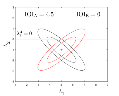
To further demonstrate the second point above, we show in Fig. 5 two toy experiments. These two toy experiments have the same mean of (here it is the second element of ), but they have different means in . If we marginalize over , we will make the two experiments look more consistent with each other as shown in the right panel of Fig. 5. This is because in this case both experiments have broad marginalized uncertainties in , but the actual degeneracy direction of the experiments is not along the direction of . Marginalizing over hides the fact that the two experiments actually have little overlap shown in a higher dimension. This effect is caught by the drop in IOI. The total IOI is meaning a significant inconsistency between the two toy experiments, but after marginalizing over , IOI becomes meaning no significant inconsistency.
From the above discussion, we can see that parameter marginalization hides experimental inconsistency when present. We need to explore the following two questions. Does IOI always drop after parameter marginalization when it should? When marginalizing over a parameter that has no inconsistency associated with it and it does not correlate with other parameters, then IOI remains the same after marginalizing over that parameter. We find that it is case if those two conditions are satisfied. We prove analytically in Appendix B.1 that IOI never increases after parameter marginalization. The general condition for IOI to remain the same after marginalizing over is,
| (16) |
where ’s are the elements of , and is a matrix obtained by taking out the kth row and kth column from . If two experiments give the same mean value of (i.e. ), and if does not correlate with other parameters (i.e. for ), the equality condition [Eq. (16)] is satisfied since both sides are . Then IOI will remain the same after marginalizing over . So IOI does track exactly the effect of marginalization. This is a unique feature of IOI among all the measures of inconsistency222In Gaussian cases, it is also a feature of and the tension..
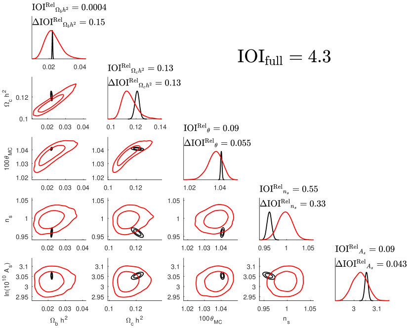
However, the condition and is only a subset of the equality condition [Eq. (16)] (although such a subset is more common and practical). Equation (16) suggests that there are some other conditions for the experimental inconsistency to be preserved after parameter marginalization. The equality condition (16) can be satisfied without or . An example of such situation and a full discussion are provided in Appendix B.3. In other words, if the drop of IOI after marginalizing over one parameter is small, it does not necessarily mean we are safe to marginalize over that parameter. As we discuss in the next section, we should also check whether the residual IOIi after marginalizing over all the other parameters is also small. If both are small, we can marginalize safely over that parameter to analyze the inconsistency for the remaining parameter space of the model.
| Notations | Meanings | Relative measures |
|---|---|---|
| IOIi | The residual IOI after marginalizing over all the other parameters except | |
| IOIi | The drop of IOI after marginalizing over |
VI Zooming on one parameter: relative drop in IOI and relative residual IOI
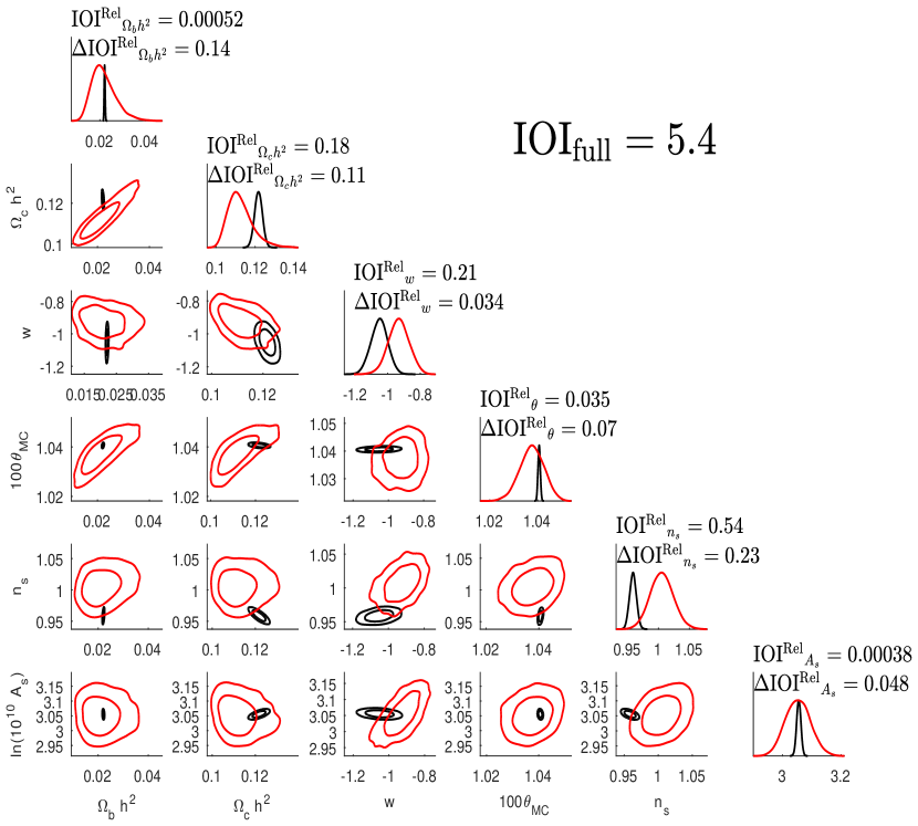
The usual way to zoom the experimental inconsistency of a given parameter is to plot and compare the two marginalized 1D likelihoods in the same graph. Examples are the marginalized 1D plots in Fig. 10 and Fig. 11 in Sec. XI. As we show in Sec. V, this is not an accurate description of experimental inconsistency. An important point is that parameters are correlated with each other (in the language of IOI, the correlation is specified by the combined covariance matrix instead of , or the joint covariance matrix ), but marginalized 1D plots do not reflect this fact. So if the two experiments yield a consistent result on one parameter in this way, it does not mean it is safe to marginalize such parameter and analyze the inconsistency of the other parameters. Even all marginalized 1D plots show quite consistent constraints on all parameters; it does not mean the two experiments are actually consistent with each other. Adding a measure to a 1D marginalized plot does not improve the situation at all, because a numerical value associated with a 1D plot does not reflect the effect of marginalization either. All the above points suggest that the usual way of viewing the experimental inconsistency of parameters in marginalized plots is not accurate, and a measure of inconsistency for the full parameter space should be used.
On the other hand, we still want to see if two experiments agree on one particular parameter. For example, we want to see if the geometry and the growth sets of experiments give consistent properties of dark energy as its equation of state . For IOI, an (obvious) one-parameter inconsistency IOIi can be defined as the residual IOI of parameter after marginalizing over all the other parameters in the model. But as we show below, this IOIi does not fully specify the inconsistency due to parameter . Indeed, to better specify the inconsistency due to one particular parameter in a model, we propose a supplemental measure based on IOI. We define the drop of IOI after marginalizing over itself, that is
| (17) |
This definition is motivated by the fact that IOI never increases whenever we perform a parameter marginalization. Since other measures may increase in general, this supplemental measure of one-parameter inconsistency is unique among the other measures in the literature.
With the two measures of one-parameter inconsistency, we can see if it is safe to marginalize over a parameter to analyze the experimental inconsistency. The residual IOIi can be directly associated with the corresponding marginalized 1D plot, while the drop IOIi can tells us the degree of inconsistency hidden by marginalizing over . If two experiments do not have inconsistency due to , both IOIi and should be small on Jeffreys’ scales. On the other hand, if one of them is large, it means there exists inconsistency associated with that parameter, and it is not safe to marginalize over it to analyze the inconsistency of the other parameters. In Sec. B.3 we describe in detail different situations regarding different magnitudes of IOIi and , and we summarize them in Table 12. In sum, marginalizing over a parameter that has a large IOIi or IOIi will either hide the inconsistency due to correlation or ignore the shape of the original distributions. The requirement is that both measures must be small.
The two measures of one-parameter inconsistency IOIi and IOIi can be compared to Jeffreys’ scales (Table 3). However, we often have situations where all IOIi’s and IOIi’s are not significant on Jeffreys’ scales but they are still not insignificant compared to the full IOI. In this situation, it is not good to marginalize over any parameter to analyze the experimental inconsistency. Therefore, when we decide whether we can marginalize over a parameter, we can compare IOIi and IOIi to the full IOI. For that, we define the relative residual and relative drop for the parameter ,
| (18) |
Both and need to be much smaller than 1 for us to safely marginalize over . The definitions of the two measures of one-parameter inconsistency are summarized in Table 4.
Note that the summation of all IOIi’s or IOIi’s is not the full IOI. That is
| (19) |
Consequently,
| (20) |
Thus we cannot interpret or as the fractional inconsistency for . Normalizing and by deriving the full IOI is only a way to see whether the inconsistency due to is significant to the full inconsistency of a model.
VII IOI eigen-mode decomposition
Since IOI is in a quadratic form, it possible to define eigenmodes of inconsistency as the eigenmodes of the matrix . By diagonalizing we obtain eigenmodes with eigenvalues . Note that the eigenmodes are characterized by , instead of in the usual principal component analysis. Suppose is the orthogonal transformation matrix from the original parameter space to the eigenmodes, i.e. and , then Eq. (9) in the eigenmodes of reads,
| (22) |
From the above equation, we can see that the full IOI is a summation of terms, each of which involves the mean difference of one and only one eigenmode parameter. We can then identify each term as the inconsistency of each eigenmode parameter, i.e. IOI (assumed in a descending order), and we have
| (23) |
A nice feature of the inconsistency eigenmodes is that these IOI’s are equal to the drop IOIi after marginalizing over the corresponding parameter, and also are equal to the residual IOIi of after marginalizing over all the other parameters, that is
| (24) |
Recall Eqs. (23) and (24) are only valid for eigenmodes of inconsistency. In general cases, the summation of ’s or ’s does not equal IOI of the full parameter space.
Let us further clarify the meaning of inconsistency eigenmodes. First, this is not like the principal component analysis in which the uncertainties of eigenmodes are specified by the eigenvalues of a Fisher matrix. Here the eigenmode inconsistency is specified by IOI, rather than alone. A larger does not necessarily mean a larger inconsistency. Second, if we rotate the parameter space and make one parameter along the deviation vector , we can express the full IOI as , where (or ) is the diagonal element of the rotated corresponding to the deviation direction, and is the magnitude of the deviation vector. So the largest inconsistency “mode” seems to be just along the deviation vector . However, the numerical value of is not preserved after marginalizing over other parameters. It is the element that is preserved after marginalization. And since is not in general, changes its value after marginalizing over any other parameter. In contrast, the eigenmodes of inconsistency here have a feature that each IOI is preserved after marginalizing over any other parameter.
VIII IOI in nested models (fixing parameters)
We have shown that marginalization can hide experimental inconsistency and lowers IOI, but it does not mean that models with more parameters will necessarily have a higher IOI. Especially if model A is nested in model B (or alternatively said, model B is an extension to model A), it does not necessarily mean model B will have a higher IOI than model A. It was shown in Ref. Verde et al. (2013) with their own measure called the tension that extending a model does not necessarily increase or decrease experimental inconsistency. Here we use IOI to show this point in an explicit way. If model A is nested in model B, one (some) of the parameters in model B is (are) fixed in model A. This actually has two effects on the likelihoods. First, fixing a parameter will take out the corresponding elements from the Fisher matrices of model B, and the covariance matrices and consequently the matrix will be changed. Second, the mean values are forced to be shifted onto a parameter subspace of one (or some) constant parameter(s). These two effects can be shown more explicitly with an example in two dimensions. We assume that the extension model B has means and from two experiments), and Fisher matrices and . When we fix, e.g., to , for each likelihood we can manipulate the term as follows:
| (25) |
where is the element of . After taking the exponential of the above, the terms independent of become only a multiplying factor that can be taken care of by normalization. So fixing parameter to changes the squared uncertainty of from to , and shifts the means of from to .
The shifts of means change IOI the most: it may either bring the means closer or push them fartheraway. As a result, an extension may have a larger or smaller IOI than the model being extended. Figure 6 shows the two possibilities. In both panels in Fig. 6, model B is an extension to model A. Model B has two parameters, and . Parameter is fixed to in model A. In the left panel, the two toy experiments give two consistent distributions for model B, and IOIB is . But since we fix to , the distributions are now on the straight line. The two means are now pushed farther apart in model A. The extension model B is more consistent than model A when comparing the two experiments, and accordingly IOIB is smaller than IOIA. On the other hand, in the right panel the means are brought closer when fixing to . The extension model B is then less consistent than model A, and IOIB is accordingly larger than IOIA. Therefore, an extension may have larger or smaller IOI.
We classify model B to be either a more consistent extension to model A (if IOIB is smaller than IOIA), or a less consistent extension (if IOIB is larger than IOIA). But since IOI depends on particular experiments, whether an extension is more or less consistent is relative and depends on the experiments under consideration.
IX Nuisance and unshared parameters
When we compare two experiments, we often come across situations where one experiment can constrain some parameters in a model but the other cannot, or each experiment has its own systematic/nuisance parameters. In those situations, the two experiments give two probability distributions with different parameter dimensions. It is then necessary to marginalize over the uncommon parameters to get two distributions with the same dimension. Does parameter marginalization in these cases hide some experimental inconsistencies? The answer is no. Marginalizing over any systematic parameters or unshared parameters does not affect IOI even in the case where the inconsistencies can be caused by those parameters.
For a real example, in Sec. XI we will compare the geometry experiments and the growth experiments in the CDM model. Since the geometry experiments do not constrain the parameter (optical depth), we need to fix it when fitting the CDM model to the geometry experiments. We then marginalize over for the growth experiments to compare the two sets of experiments. If the geometry experiments do not constrain or very poorly constrain , it is equivalent to the situation as follows: (1) where it gives very wide (weak) uncertainty on , and ; (2) where has no correlation with other parameters in the geometry set, and for . No matter what constraint of is given by the growth experiments, the geometry experiments do not “object” to such a constraint, and there is no conflict between the two sets on the value of . This does not necessarily mean that the joint mean of would be the same as the mean given by the growth experiments. In fact they are different in general, and the joint mean is given by the Fisher-matrix-weighted average [Eq. (7)]. However, the form of now implies that the joint mean of does not depends on the fixed value of for in geometry set, or the mean given by the geometry set (if it gave one).
Mathematically, we can see more clearly from the analytical expression of IOIτ given by Eq. (93). If for and , we have . Every term in Eq. (93) is finite except for . So the denominator of Eq. (93) goes to and IOI. In another word, the drop of IOI after marginalizing over is . Also IOI as well since and IOI for finite . Since both IOIτ and IOIτ are zero, there is no problem to marginalize over to analyze the inconsistency of the whole model. For the same reason, it is also safe to marginalize over all the nuisance parameters of each experiment.
X Comparison with other measures of inconsistency in the literature
In this section we compare IOI to some other measures of inconsistency/consistency in the literature. Their Gaussian and weak prior limits will be derived for the comparison. We also examine how such measures track or not inconsistencies in various particular cases.
X.1 The robustness
The robustness was introduced in Refs. Marshall et al. (2006); March et al. (2011), and has been applied, e.g., in Ref. Amendola et al. (2013) to investigate the internal inconsistency of type Ia supernovae data set. It is defined as the Bayesian evidence ratio between the combined model and the split model in order to quantify the consistency between two experiments as follows. Combined model: the two experiments are jointly fit by a set of parameters; Split model: each experiment is individually fitted by one set of parameters. The robustness is then defined as
| (26) |
where is the corresponding Bayesian evidence, so
| (27) | ||||
| (28) | ||||
The values of are interpreted by Jeffreys’ scales listed in Table 5.
| Ranges | ||||
|---|---|---|---|---|
| Meanings | No preference | Weak evidence | Moderate evidence | Strong evidence |
In the Gaussian limit, we can calculate the robustness analytically. Different from the treatment in Ref. March et al. (2011), we do not set one of the means to be to find
| (29) |
where,
| (30) |
The major steps of the above calculation can be found in our Appendix A.3. In the weak prior limit Eq. (29) can be further reduced to,
| (31) |
So the robustness in the case of Gaussian and weak prior is related to the negative of IOI with an additional term that accounts for the Occam’s razor factor (favoring the model with fewer assumptions). A similar relation [to Eq.,(31)] is pointed out in Ref. Marshall et al. (2006) where is related to (same as with our notation) which in the Gaussian case is defined as IOI in this work. Ref. Seehars et al. (2016) noted that the dependence of prior does not go away in the weak prior limit and diverges as . This seems to imply that two experiments are always consistent with each other when a very weak prior is used, which cannot be true.
The dependence of can be eliminated by a normalization. So for example, the authors of Ref. March et al. (2011) define where , so that if the second experiment gives the same likelihood as the first one. Then from Eq. (31), in the Gaussian and weak prior limit reads
| (32) |
and the dependence on is eliminated. But other problems seem to persist. For example, consider two Gaussian likelihoods with the same mean, i.e., . And suppose their Fisher matrices are given by
| (33) |
Similar likelihood contours of these two toy experiments are shown in Fig. 4, but now the contours are much narrower. The first constraint ellipse is very elongated along the direction, while the other is very elongated along the direction. Although there is little overlap between the two experiments, they have the same parameter mean so there should be no tension between them333A real and similar example of this situation is the experiments of BAO and distances to supernova.. But the normalized robustness turns out to be (to the leading order of )
| (34) |
So implies these two toy experiments are not “robust” or not consistent with each other, which seems to be in contradiction with the fact that they are actually consistent with each other.
The term in the original robustness also disfavors orthogonal constraints. It may be easier to see this if we relate the robustness to IOI and FOM. From the Gaussian and weak prior limit of the robustness [Eq. (31)] and the definition of FOM [Eq. (15)], we can see that
| (35) |
where the subscripts“”, “”, “” and “” stand for “first”, “second”, “joint” and “prior”. In Sec. IV we argued that different constraint orientations do lead to different experimental inconsistencies, which have already been taken care of by IOI. For a fixed FOMp, the term can describe how powerful the joint constraint is compared to the two individual constraints. It is true that this term does also depend on the constraint orientations, and it is larger for orthogonal constraints than parallel constraints. But it should not be taken into accounted as indication of consistency or inconsistency, because it is independent of how far away the two individual constraints are separated from each other.
X.2 The Tension
Based on Bayesian evidence ratio, a quantity called the tension was introduced in Ref. Verde et al. (2013). This measure was used in Ref. Bernal et al. (2016b), e.g., to study the tension between the direct measurement of and the one derived from Planck CMB observation. The is defined as follows. For two posteriors and , we transfer them while keeping their shapes to get two new posteriors and . Peaks of and coincide at the same location. Then the tension is defined as
| (36) |
As Ref. Verde et al. (2013) explained, the tension is defined as the joint Bayesian evidence ratio between a virtual hypothesis and an actual hypothesis. It was also proposed in Ref. Verde et al. (2013) to interpret using Jeffreys’ scales.
In the case of Gaussian likelihoods and a Gaussian posterior, the integral of the posterior product in Eq. (36) can be calculated analytically (see our Appendix A.3 for details)
| (37) |
where (again) , , , and . Note that and are different from and , and the former ones have the prior involved. In the weak prior limit, and . The shifted-posterior-product integral is similar except that , so . Therefore, the tension becomes
| (38) |
So reduces to IOI in the Gaussian and weak prior limit. Since the shifted posteriors always have a larger overlapping region for Gaussian cases, , which can also be seen from Eq. (38).
It was also shown in Ref. Verde et al. (2013) that the tension is another information for the problem of model selection. For example, Table 2 in Ref. Verde et al. (2013) shows that while there is not enough Bayesian evidence favoring the CDM model over the CDM model, the latter significantly reduces the tension on between the Planck and the local measurements.
Authors in Ref. Seehars et al. (2016) commented that the tension is of the order (dimension of the parameter space) and could overestimate the inconsistency between two experiments. Since and IOI are the same in the Gaussian and weak prior limit, that comment would also apply to IOI. But we find here otherwise. First, Table 2 in Ref. Verde et al. (2013) showed that some extensions of the CDM model increase the tension while the others decrease it. So increasing the degree of freedoms does not necessarily increases or decrease . Second, we can always rotate the parameter space and let the first axis be along the deviation vector . Then consists of only one term in the Gaussian and weak prior limit (see Sec. VII). So it should be of the order unity.
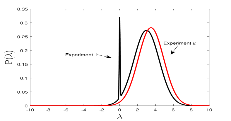
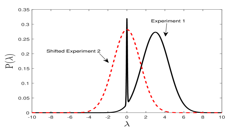
While the tension reduces to IOI in the Gaussian and weak prior limit, the difference between them lies in non-Gaussian cases and in the fact that they originate from distinct concepts (see Table 7). One advantage of the tension compared to IOI is that the tension is defined for general distributions. The tension may give us a better sense of inconsistency in general cases (although we do not know yet what a good measure is in non-Gaussian cases), while IOI may not work in highly non-Gaussian cases. However, in some cases, it may be better to use IOI. Recall that the definition of the tension involves the shifted distributions such that they have coinciding maxima. This may give to the tension an ambiguity in choosing the shift in general cases. Consider the two 1D distributions shown in the upper panel of Fig. 7. The two experiments give two similar distributions. But is not Gaussian, and it has a narrow peak at which is unfortunately also the maximum of . If we shift the two distributions to make their maxima coincide, we will get the lower panel in Fig. 7. Since the shifted distributions have less overlap than the original distributions, the numerator in Eq. 36 can be smaller than the denominator. We can then get and . The negative value of here certainly cannot be interpreted as ‘no tension’. In fact, the ‘majorities’ of the two distribution may be very different and exhibit a large tension, but may still be negative due to the possibly small overlap of the shifted distributions. The problem is that the numerator in Eq. (36) is not guaranteed to be larger than the denominator. Better shifted distributions can be defined as those who maximize the numerator in Eq. (36), though such definition may not be as practical as the original one. However, distributions in cosmology are usually unimodal, making two maxima to coincide usually also maximize the numerator in Eq. (36). Our extreme example here is only to show the possible ambiguity in the choice of distribution shift for general cases, but the measure tension should work just fine in the usual and common cases.
X.3 The discordance
The discordance was constructed from overlapping iso-likelihood contours and was proposed in Ref. MacCrann et al. (2015) to measure the inconsistency between two distributions in the following way. First, for a given specific percentage, we can draw two iso-likelihood contours of the two distributions. Depending on how far away the two distributions are separated from each other, the two iso-likelihood contours may or may not overlap. If the two distributions are very far away from each other, the two iso-likelihood contours need to be large (corresponding to a large included percentage) in order to overlap with each other. So the percentage within each overlapping iso-likelihood contours traces the distance of two distributions. The discordance is defined as the minimum percentage of the overlapping iso-likelihoods that include equal probability. A larger corresponds to a greater distance between the two distributions, and a larger inconsistency. If the maxima of two distributions coincide at the same location, will be ; on the other hand if they are separated very far away and very inconsistent with each other, . The range of discordance is , and it is compared to to measure the level of inconsistency.
Reference MacCrann et al. (2015) also discussed the effect of marginalization on the value of discordance. But instead of decreasing after marginalization, the discordance tends to increase. In their Appendix A (in Ref. MacCrann et al. (2015)) they showed a simple example of 2D toy experiments. Both of their toy experiments provide uncorrelated parameter constraints. While the two experiments give different mean values of parameter , the means of are the same. After they marginalize over , the discordance increases. This is different from the behavior of IOI and what we have shown graphically in Sec. V. We have argued that marginalizing over inconsistency-irrelevant parameters444Parameters that have the same mean values and do not correlate with other parameters, or unshared parameters does not affect the study of inconsistency between two experiments. In their example the two mean values of the are the same, and there is no correlation between and , marginalizing over should not change the inconsistency between the two toy experiments or the measure representing it. It was suggested in Ref. MacCrann et al. (2015) that, for a model with dimensions, it is the full -dimensional that should be used for a conservative measure of discordance. However, if two experiments have inconsistent results on only one parameter and if all parameters are uncorrelated, a model with a higher dimension will have a smaller discordance. In that case, a very high-dimensional model will have a very low discordance. The full-parameter discordance actually underestimates the inconsistency in that case.
Unlike for the other measures, we could not obtain an explicit expression of the discordance. However, there is a simple algebraic procedure to calculate it in Gaussian and weak prior limit that we provide below. When so that the prior can be treated as a constant in the parameter range of interest, the integrated probability included within the iso-likelihood contour of the same is given by
| (39) |
where is the gamma function and is the lower incomplete gamma function. The overlapping iso-likelihoods with minimum will be tangentially touching with each other at point . The gradients of two iso-likelihoods at must be of opposite directions, that is
| (40) |
where is a number we need to solve for. In Gaussian cases with , we can get as a function of from Eq. (40), that is
| (41) |
Equation (41) can be viewed as a modified-Fisher-matrix-weighted average. There are three special cases: when ; when ; and when . By definition we have
| (42) |
We can first solve Eq. (42) for , substitute in Eq. (41) to get , and substitute in Eq. (39) to get
| (43) |
We use this algorithm to make corresponding calculations further in the paper.
X.4 The surprise
Based on relative entropy (or Kullback-Leibler divergence) in information theory, a measure, called surprise, was introduced in Refs. Seehars et al. (2014, 2016); Grandis et al. (2016a). Reference Zhao et al. (2017) used this measure to study the tension between different distance indicators. For two posterior probability distributions, this quantity is defined as the difference between the relative entropy and its average
| (44) | ||||
| (45) |
The average above is taken over a probability distribution of the second data given the first data :
| (46) | ||||
| (47) |
The uncertainty of can also be calculated,
| (48) |
And the significance of is defined as
| (49) |
Two different cases are discussed in Ref. Seehars et al. (2014): one is called “updating data” where the second experiment is used to updated the constraints from the first experiments as a prior; the other is called “replacing data” where two experiments are used separately to set constraints on parameters. Since we are considering the inconsistency between two experiments with similar constraining powers, it is the second case that is more relevant to our work. The surprise and for the second case in the Gaussian limit is given in Ref. Seehars et al. (2016), which in our notation read
| (50) |
| (51) |
where is the -dimensional identity matrix. The relative entropy (and the surprise) is divided by when being measured in the unit of bits. For example, if the second experiment only gives a narrower constraint than the first one, roughly means that the second experiment improves and shrinks the constraint to half compared to the first experiment .
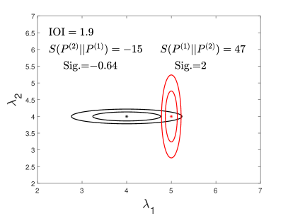
Despite its interesting concept, the outcome of the surprise seems to depend on the choice of its argument order leading to some ambiguity. For example, let us consider two sets of toy experiments described by
| (52) | |||
| (53) | |||
| (54) | |||
| (55) |
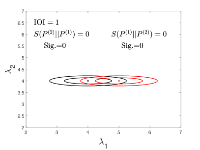
These two sets of experiments are shown in Fig. 8.
The contour plots indicate that the two experiments shown on the left panel seem to have a smaller inconsistency than those on the right panel. This is, for example, reflected quantitatively on the respective values of IOI with the right value (i.e. 1.9) being larger than the left one (i.e. 1.0). However, if is used, it decreases from on the left to (or bits) on the right, implying a decrease of inconsistency. The significance of also has the same implication: for the left panel and for the right one. Now, since the surprise is not symmetric about the two experiments, one may choose a different argument order in . So, if we instead use (i.e., switching the argument order), the surprise and its significance changes both from on the left panel to and respectively on the right panel. It is unclear what should be a good rationalization to choose the order of arguments in . It could be argued that the choice should be physically motivated favoring the more trusted data set with less expected systematic uncertainties, thus with a prior preference of a given data set which could be viewed as consistent with a Bayesian statistics approach pri . It remains unclear though what is the right choice if both data sets have their own significant systematic errors or when the inconsistency is rooted into a problem with the model or the theory itself.
Finally, the surprise and its significance are found to increase after parameter marginalization in, for example, the following toy experiments:
| (56) |
which are shown also in Fig. 9. We argued in Sec. V that should not be relevant to the inconsistency, because the two experiments have the same mean of and there is no correlation between and . So after marginalizing over a measure of inconsistency should be preserved, as is the case for IOI. As shown in Fig. 9, before marginalizing over , the surprise (and its significance) is . After marginalizing over , it becomes with a significance of . It can be argued this is a normal behaviour for the surprise because the results of are more consistent than expected pri . So marginalizing over emphacises the inconsistency in and that is reflected by the increase of the marginalized surprise pri . But then when going from the right to the left panel, the inconsistencies as indicated by the values of the surprise and its significance on the left seem to go away. It is unclear if this is really the case since the inconsistency in is still present.
X.5 The calibrated evidence ratio
Reference Grandis et al. (2016b) introduced the calibrated evidence ratio (CER hereafter) by calibrating the robustness using its average. The level of CER can also be described by its significance. But different from the case of the surprise, the average here is taken over a probability distribution of both the first and the second data and , which is given by the joint evidence ,
| (57) | ||||
| (58) |
In Gaussian cases, CER in dimensions is given by
| (59) | ||||
| (60) | ||||
So the opposite of CER is related to IOI in the Gaussian and weak prior limit by an additive constant, .
The CER measure did address some of the issues with its predecessors. It is worth noting though that since IOI is positive definite, is the minimum value of CER. Because of the term , CER can be be more negative with higher dimensional parameter spaces. The significance defined as CER goes as when IOI . The term (and for its significance) seems to suggest that a model with a higher dimension tends to have a smaller inconsistency. It can be argued that this is normal because a higher dimensional model allows larger scatter of the data, which leads to a larger expected pri . Consider though the following situation: if two experiments have inconsistency on only one parameter (e.g., ) and if all parameters are uncorrelated, a model with a higher dimension will have a smaller CER. This seems to underestimate the inconsistency that is due to one particular parameter.
| Quantities | Symbols | Relevant concept | Gaussian and weak prior limit |
|---|---|---|---|
| Index of inconsistency | IOI | (definition) | |
| Robustness Marshall et al. (2006); March et al. (2011) | Bayesian evidence ratio | ||
| Normalized robustness March et al. (2011) | Bayesian evidence ratio | ||
| Tension Verde et al. (2013) | Bayesian evidence ratio | ||
| Discordance MacCrann et al. (2015) | Iso-likelihood contour | Algorithm provided by Eqs. (41)-(43) | |
| Surprise 555The case of replacing data described in Ref. Seehars et al. (2014) is used in this work. Seehars et al. (2014, 2016); Grandis et al. (2016a) | Relative entropy | ||
| and its deviation | |||
| Calibrated evid. ratio Grandis et al. (2016b) | CER | Bayesian evidence ratio | |
| and its deviation | |||
| Level of concordance Joudaki et al. (2017) | Deviance information criterion |
| Quantities | Symmetric? |
Follow
inconsistency? |
Give 0
if ? |
Reflect effects of
marginalization? |
Proposed interpretation |
|---|---|---|---|---|---|
| IOI | ✓ | ✓ | ✓ | ✓ | Jeffreys’ scales |
| Robustness | ✓ | ✗ | ✗ | N/A | Jeffreys’ scales |
| Normalized | ✗ | ✗ | ✗ | ✗ | Not specified |
| Discordance | ✓ | ✓ | ✓ | ✗ | Compared to |
| Surprise | ✗ | ?666Due to the asymmetric behavior, if the surprise has the wrong choice of argument order, the trend will be incorrect. | ✗ | ✗ | Bits significance |
| CER | ✓ | ✓ | ✗ | N/A | Significance |
It is also worth mentioning that from Eq. (59) we can see, in the Gaussian and weak prior limit, CER has a close relation with the Akaike information criterion Akaike (1974) for the following reason. The Akaike information criterion (AIC) is to select a model with a smaller AIC. For a model with parameters, the corresponding splitting model has parameters. The AIC difference between the combined and the split models is
| (61) |
X.6 Level of concordance
Analogous to the robustness, Ref. Joudaki et al. (2017) most recently introduced the level of concordance, defined as , to measure experimental (in)consistency. Instead of using the Bayesian evidence ratio between the combined and the split models, uses the deviance information criterion (DIC) (see Refs. Spiegelhalter et al. (2002); Liddle (2007)), and it is defined as
| (62) |
where DIC, and is the effective number of parameters given by . Jeffreys’ scale was used to interpret this measure.
Since DIC approaches AIC in the Gaussian limit (when parameters are well constrained) Liddle (2007), is equivalent to CER (see Sec. X.5 for the connection between CER and AIC) in Gaussian limit, i.e.,
| (63) |
Therefore, level of concordance measure seams to share the points mentioned above for the CER.
X.7 Is there a connection between IOI, Surprise and CER
The definitions of the robustness , tension , surprise , CER and IOI are quite different. But we have seen in the previous sections that , and CRE are related to IOI by equations (31) & (32), (38) and (59). Is there a relation between the surprise and IOI? We find that only in one dimension the significance of the surprise is simply related to IOI, and to the significance of CER.
In one dimension with Gaussian and weak prior, the surprise given by Eq. (50) reduces to
| (64) |
the deviation of reduces to
| (65) |
and the significance is given by
| (66) |
In one dimension, the significance of the surprise becomes symmetric about two experiments. IOI in this case is given by , and from (59) and (58) we can obtain the significance of CER in this case as , for . Therefore the three quantities are related by
| (67) |
In dimensions, due to the connection of CER to AIC, the relation between IOI and CER (and its significance) remains simple in the Gaussian and weak prior limit, and it is given by Eq. (59), and
| (68) |
But it is not obvious to see the relation between IOI and surprise. The surprise and its significance become asymmetric for two- or multiple-dimensional parameter spaces, while IOI is always symmetrical.
XI Application of IOI to cosmological experiments: geometry vs growth
To test the internal consistency of the CDM and CDM models, we fit each of them separately to a set of geometry experiments and a set of growth experiments. This is partly motivated by the fact that different theories (e.g. modified gravity) have relations between the cosmic expansion background and the large scale structure growth, e.g. Ishak et al. (2006). We use the publicly available Markov Chain Monte Carlo code CosmoMC Lewis and Bridle (2002) for parameter constraints. Note that, in this work, we will not use IOI for multiple experiments [see Ref. (12) to study the full experimental inconsistency among them. Rather, we will treat the geometry experiments as one set of experiments and the growth experiments as the other set, and then apply IOI to measure the (in)consistency between the two set of experiments [Eq. (9)].
| Geometry | Growth | ||
|---|---|---|---|
| Supernovae Type Ia Betoule et al. (2014) | Planck 2015 low- CMB temperature and polarization Ade et al. (2016a) (Planck Collaboration) | ||
| BAO | Six Degree Field Glactic Survey (6dF) Beutler et al. (2011) | Planck 2015 CMB lensing Ade et al. (2016b) (Planck Collaboration) | |
| SDSS main galaxy sample (MGS) Ross et al. (2015) | Sunyaev–Zel’dovich effect Ade and others (2016) (Planck Collaboration) | ||
| SDSS quasar-Lyman- forest Aubourg et al. (2015) | CFHTlens galaxy weak lensing Heymans et al. (2013) | ||
| Planck 2015 High- CMB temperature Ade et al. (2016a) (Planck Collaboration) | RSD | WiggleZ Dark Energy Survey Blake et al. (2010); Parkinson et al. (2012) | |
| SDSS DR12 CMASS and LOWZ catalogs Alam et al. (2015) | |||
| Measures | IOI | 777“gm” “geometry”, “gr” “growth”. | Significance | Sig. | CER | Sig. | |||
|---|---|---|---|---|---|---|---|---|---|
| CDM | |||||||||
| CDM |
XI.1 Data sets
For the geometry set of experiments, we use the type Ia supernovae catalog compiled in Ref. Betoule et al. (2014), the baryon acoustic oscillation (BAO) standard ruler from the Six Degree Field Glactic Survey (6dF) Beutler et al. (2011), the main galaxy sample (MGS) of data release seven (DR7) from the Sloan Digital Sky Survey (SDSS) and the SDSS quasar-Lyman- forest Aubourg et al. (2015), and the high- CMB temperature data from Planck 2015 Ade et al. (2016a) (Planck Collaboration). For the growth set of experiments, we use the low- CMB temperature and polarization data from Planck 2015 Ade et al. (2016b) (Planck Collaboration), CMB lensing Ade et al. (2016b) (Planck Collaboration), thermal Sunyaev-Zel’dovich effect Ade and others (2016) (Planck Collaboration), galaxy weak lensing cosmic shear from the Canada France Hawaii Lensing Survey (CFHTlens) Heymans et al. (2013), and the redshift space distortion from the WiggleZ Dark Energy Survey (WiggleZ MPK) Blake et al. (2010); Parkinson et al. (2012) and the SDSS DR12 CMASS and LOWZ catalogs Alam et al. (2015). Those two sets of experiments are summarized in Table 8. Note that we put high- CMB temperature data in the geometry set as in Ref. Bernal et al. (2016a), since its acoustic peaks strongly constrain the expansion history of the Universe.
From Table 8 we can see that there are some overlaps between the data sets used in this work and those used in Refs. Bernal et al. (2016a); Ruiz and Huterer (2015). But there are some differences. First, for the RSD data from SDSS, while Ref. Bernal et al. (2016a) separately used the measurements of and as geometry and growth sets, we use them all in the growth set because these two measurements (as well as ) are correlated. Second, we use the full data catalog of RSD from WiggleZ, while Ref. Bernal et al. (2016a) used its compressed information on BAO and growth. Third, we use the combined Lyman- BAO data at from Ly forest autocorrelation and the quasar-Ly cross-correlation Aubourg et al. (2015), while Ref. Bernal et al. (2016a) only used the data from cross-correlation.
XI.2 Results from application to data: A moderate to strong inconsistency
For the CDM model, we use the following parameters: , , , , , and (for the (CDM) we add ). We fit each model separately into the geometry set and growth set of experiments listed in Table 8. Since the geometry experiments poorly constrain , we set it to the mean value obtained in Ref. Adam and others (2016b) (Planck Collaboration) , while we allow it to vary in the fitting of the growth experiments. The constraints from the two sets of experiments are shown in Figs. 10 and 11. To quantify the inconsistency between the geometry and the growth experiments, we calculate IOI for the full parameter space (marginalized over ). Additionally, to compare IOI to the other measures of inconsistency, we also calculate other measures in the Gaussian and weak prior limit, like the normalized robustness , the discordance, the surprise and (and their significance) and the CER (and its significance). All results of inconsistency between the geometry and the growth experiments for the CDM and CDM models are listed in Table 9.
We can see from Table 9 that all the measures (except for ) overall suggest there are inconsistencies between geometry and growth data sets for CDM and CDM models. However, different measures provide different levels of inconsistency. Take, for example, the CDM model. IOI suggests a moderate experimental inconsistency (in fact not too far from a significant one on Jeffreys’ scales). We note that the normalized robustness gives an inconsistency much higher than other measures and ranked as very strong (decisive) if we insist to interpret it in Jeffreys’ scales. However, this high inconsistency using the normalized robustness is artificial as we explain. The geometry experiments give much stronger constraints than the growth ones, so that , and the term . Therefore the apparent inconsistency suggested by is only due to the unmatched constraining powers of the two data sets. The quantity CER is simply related to IOI by Eq. (59). It is suggested in Ref. Grandis et al. (2016b) that CER should be interpreted in terms of its significance. The significance of CER gives a confidence level of inconsistency of . For the surprise, different orders of experiments in its argument lead to different results. While is positive and finite, is negative and large. The significance of the surprise also has such asymmetric problem. While the significance of gives no inconsistency, the significance of suggests inconsistency, which seems more consistent with the one suggested by IOI and Fig. 10. The value of discordance is . Compared with , the discordance also seems to suggest some inconsistencies.
Comparing the results between CDM and CDM models, we can see that all measures (except for ) suggest that the CDM model has a larger inconsistency regarding the geometry and the growth experiments. In the language of IOI in nested models (see Sec. VIII), we say that the CDM model is a less consistent extension to the CDM model when comparing growth versus geometry. The result that the CDM model has a larger experimental inconsistency is different from what was found in Ref. Verde et al. (2013). This may not be surprising, because Ref Verde et al. (2013) were comparing Planck with local measurement on the Hubble constant and the age of the Universe, which are different experiments from what we are considering. The values of inconsistency measures are experiment dependent. Reference Di Valentino et al. (2017) also found that the CDM model is more favored than CDM model when Planck, the local measurement of and BAO datasets are analyzed jointly. Indeed, when IOI is applied to investigate the inconsistency between Planck and local measurement on , we find IOI for CDM and for CDM. These numbers are consistent with those provided in Table 2 in Ref. Verde et al. (2013) (recall that IOI and the tension are the same in the Gaussian limit). So CDM does have a smaller IOI in this case. However, the reason might be simply that Planck data have a poor constraint on if is allowed to vary; km/s/Mpc. Recall that one of the three factors affecting IOI is the constraint volume: a larger constraint volume leads to a smaller IOI.
| CDM parameters | |||||
|---|---|---|---|---|---|
| IOIi (IOI) | () | () | () | () | () |
| () | () | () | () | () | () |
| (significance of ) |
| CDM parameters | ||||||
|---|---|---|---|---|---|---|
| IOIi (IOI) | () | () | () | () | () | () |
| () | () | () | () | () | () | () |
| (significance of ) |
Finally in this subsection, we briefly investigate the roles of CFHTlens data and SDSS RSD data on the value of IOI for CDM model. If we remove CFHTlens data alone, IOI drops from to . If we remove SDSS RSD data alone, IOI drops from to . Although the CFHTlenS data seem to cause more inconsistency, neither removing the CFHTlenS data nor the SDSS RSD data dramatically drops IOI. Therefore, the inconsistency between the geometry and the growth experiments does not seem to be caused by one particular data set. Furthermore, if we remove both CFHTlens and SDSS RSD data, IOI drops from to , but a weak inconsistency still persists. In a follow-up work, we will systematically explore the internal and cross inconsistencies between a number of data sets and more applications of IOI.
XI.3 Relative drop of IOI and relative residual IOI in the geometry vs growth application
We have shown that parameter marginalization can hide experimental inconsistency in Sec. V. This is reflected by the drop of IOI after marginalizing over each parameter, which is shown in Tables 11 and 11. The fact that IOI never increases offers us two ways to see the experimental inconsistency due to a particular parameter, which we apply here to the geometry and growth experiments.
The two measures of one-parameter inconsistency IOIi and described in Sec. VI can help us zoom into the parameter space, to see experimental inconsistency due to each parameter. For a given model, if two experiments do not have inconsistency due to , both IOIi and IOIi are small in Jeffreys’ scales. But in some cases, even though IOIi and IOIi are small in Jeffreys’ scales, they are not negligible compared to the full IOI. So more conveniently, we can use the relative quantities IOI and IOI, and compare them to unity to see the role of each parameter on experimental inconsistency. Only when both IOI and IOI are much smaller than , can we safely marginalize over to analyze the full inconsistency. We listed the two measures and their relative measures in Tables 11 and 11 for the CDM model and the CDM model, respectively.
Take the CDM model for example, the geometry and the growth experiments have a significant (full) inconsistency (IOI=5.4). For individual parameters, the 1D marginalized plots in Fig. 11 seem to show little inconsistency in , and , and the corresponding IOIi’s (and IOI) are small. But it does not mean it is safe to marginalize over these three parameters. For example, IOI is not much smaller than , so marginalizing over will hide some experimental inconsistency due to its correlation with the other parameters (specified by ). On the other hand, since both IOI and IOI are small, the geometry and the growth experiments give a consistent result on , and it is safe to marginalize over it to study the full inconsistency. Similarly, it is also safe to marginalize over . For the CDM model, from Table 11 it seems inappropriate to marginalize any parameter to analyze inconsistency, although and seem to be least responsible for the inconsistency.
Which parameter have the most inconsistent results given by the geometry and the growth experiments? From Tables 11 and 11, we can see that for both the CDM model and the CDM model, the results of are the most inconsistent. Both IOI and IOI are large. The next inconsistent parameter should be , but the inconsistency caused by it is quite small compared to that due to .
The definition of is based on the fact that IOI never increases after a parameter marginalization. This drop of IOI represents the hidden inconsistency due to a parameter after we marginalize over it. This is a unique feature for IOI. To demonstrate it, we show as examples the drops of , and its significance after marginalizing over each parameter in the last three rows of Tables 11 and 11. We can see that their drops are not always positive, suggesting that they are not able to represent the hidden inconsistency after a parameter marginalization.
It is, however, important to emphasize that although combining ’s and IOIi’s can give us more insights into the inconsistency due to each parameter, they cannot fully describe the experimental inconsistency. It is the full IOI (recall this is not the summation of ’s or IOIi’s) for the whole parameter space that should be calculated and used.
XII Summary
The CDM model is considered to be the standard and concordance model in cosmology, but different experiments have been yielding constraints of parameters that do not perfectly agree with each other. Those inconsistencies could be caused by either systematics or the breakdown of the underlying model and theory. It is timely and important to develop tools to quantify the degree of inconsistency between different experiments.
We defined a moment-based measure that we call IOI. We suggested to interpret IOI using Jeffreys’ scales listed in Table 3. We showed that IOI tracks well the separation of the means, the volume of the covariance ellipsoids, and the orientations of those ellipsoids. We discussed criteria that must be fulfilled by measures of inconsistency. For example, the numerical value of the measure must follow the graphical inconsistency of likelihood contour plots, represent experiments with definite consistency, and correctly reflect the effect of parameter marginalization. We find that IOI satisfies all those criteria. We provided an eigenmode decomposition of IOI and also discussed the application of IOI for nested models.
We showed how marginalizing over a parameter can hide inconsistency between experiments when present. This is because every parameter can induce its own experimental inconsistency and also has correlations with other parameters. In fact, even if all marginalized distribution plots look consistent for two experiments, they might still be inconsistent. These facts show that descriptions of experimental inconsistency involving parameter marginalization is not accurate. We provided an analytical proof that IOI never increases whenever a parameter marginalization is performed but rather decreases in most cases. This work seems to be the first to quantify the loss of information on cosmological experimental inconsistency due to parameter marginalization.
In order to zoom on the inconsistency residing in a particular parameter, we defined the relative drop in IOI and the relative residual IOI for a given parameter, IOI and IOI. We explained that only when both relative measures are small can one safely marginalize over such a parameter when considering inconsistency measures. We also explained that in order to correctly quantify the inconsistency we should use the full IOI of all parameters in a model that are commonly constrained by two experiments.
We provided a comparative survey of other measures of inconsistency and their relationships, if any, with IOI.
We then applied IOI and other measures in the Gaussian and weak prior limit to quantify the inconsistency of the CDM and CDM models between geometry and growth experiments. As discussed in the previous section, IOI indicates a moderate to strong inconsistency between the two data sets when the CDM and CDM models are used with values of 4.3 and 5.4 on Jeffreys’ scales. Overall, although different measures use different scales to quantity inconsistency, most of the measures (except for ) also suggest that there are moderate to strong experimental inconsistencies in CDM and CDM models with the CDM model having a larger inconsistency between geometry and growth experiments. As we discussed in the previous section, this comparison and its results are different from two other works that compared Planck with local measurement of the Hubble constant and the age of the Universe, finding that CDM brings some reconciliation. As we explained, the values of inconsistency measures are experiment dependent, as they should.
Finally, we used the IOI measure and found that CFTlenS data, SDSS RSD data and other growth data all contribute to the inconsistency. So this seems to indicate that the inconsistency cannot be associated with a single data set. In future work, we will explore in more detail the role of each data set in the experimental inconsistencies.
Acknowledgements.
We would like to thank L. Amendola, S. Grandis, M. Kesden, L. King, E. Linder, L. Pogosian, D. Rapetti, L. Verde and J. Zuntz for useful comments. M.I. acknowledges that this material is based upon work supported in part by NSF under Grant No. AST-1517768 and an award from the John Templeton Foundation.Appendix A Derivations and proofs
This appendix provides the calculations and derivations used in this work, including those used in the definition of IOI and its relationship to other measures of inconsistency.
A.1 IOI for arbitrary numbers of experiments
We consider combination of likelihoods that do not correlate with each other. A Gaussian likelihood for the th experiment reads
| (69) |
For arbitrary number of experiments, the likelihood of a joint analysis is defined as
| (70) |
Note that is the mean of the th likelihood, not the th component of . The sum in Eq. (70) can be reduced to
| (71) |
where,
| (72) | ||||
| (73) |
and we have used the fact that . Since the last two terms do not depend on , we can combine them with , and Eq. (70) becomes
| (74) |
where,
| (75) |
So the likelihood of a joint analysis is also Gaussian [Eq. (74)], with its mean, Fisher matrix and maximum value given by Eqs. (72) - (75). The above result is also applicable to the case where one of the likelihoods is replaced by a Gaussian prior, where one of the likelihoods is replaced by a prior with and set .
Note that we have defined IOI as
| (76) |
The maximum value of the joint likelihood is
| (77) |
By comparing Eq. (75) and Eq. (77) we have
| (78) |
for multiple experiments.
It is important to emphasize that, is only a motivation for our definition of IOI. It is true that IOI and are the same for Gaussian likelihoods, but for non-Gaussian cases, we define IOI as a moment-based quantity [Eq. (78)], with given by the inverse of the covariance matrix and given by the mean of the th likelihood.
A.2 Special cases: Two likelihoods
More often we will compare two experiments to see their inconsistency. For the case of two experiments (), the right-hand side of Eq. (78) becomes
| (79) |
where and in the second last row we have used . So the above derivation [Eq. (79)] shows that Eq. (12) for IOI of multiple experiments reduces to Eq. (9) for two experiments. We will use
| (80) |
as the definition of IOI for two experiments.
A.3 Integrals of joint Gaussian distributions
The integral of a single Gaussian likelihood gives
| (81) |
With the combined likelihood given by Eq. (74), we immediately obtain,
| (82) |
Appendix B Marginalization never increases IOI
B.1 Proof
We will adopt the following notations. An element of the matrix is denoted as lowercase , while stands for a matrix obtained by taking out the th row and the th column of and multiplied by . [Then is a matrix obtained by taking out the th & th rows and th & th columns of and multiplied by .] is the determinant of . Then is the (,) cofactor . Let be the vector results from deleting the th component from .
Suppose we are to marginalize . The full IOI is , and the IOI after marginalizing over is IOI. The quantity is calculated as follows: (1) delete the first element of and get ; (2) delete the first row and the first column in and let it be ; and (3) then . What we are going to show is IOI IOImar,1, that is, .
We first make a linear parameter transformation that keeps unchanged. More explicitly, we let with a transformation matrix of the form
| (84) |
where . Then the new deviation vector reads
| (85) |
Similarly, the new matrix reads,
| (86) |
where for . So under , and stay the same, and transform as vectors, and transforms as a rank-2 tensor. To simply the proof, we further let take the following form,
| (87) |
We have used the fact that . In other words, we transform the parameter space alone the direction of , so that the other (new) parameters are the eigenmodes of in the projected (-1)-dimensional parameter subspace orthogonal to . For the proof, we will work in the new parameter space and drop the primes. In this new parameter space, we have
| (88) |
With our new matrix of the form (87), we can calculate those determinants explicitly, (let , and )
After we substitute the above determinants into Eq. (88) and cancel out , reads
| (89) |
In our new parameter space, the IOI after marginalizing over is rather easy to calculate and it is . Taking the difference between and , considering only the numerator of it, and rearranging terms, we have
| (90) |
So and marginalization never increases IOI.
The condition for IOI IOImar,1 (called equality condition from now on) is . Since we have transformed the parameter space along the axis, this equality condition is not generic. To find the generic equality condition, we first note that the right-hand side of the equality condition is invariant under the transformation. Therefore we can generalize the left-hand side to a quantity that is: (1) invariant under the transformation specified by Eq. (84), and (2) reduces to in the case when takes the form of in Eq. (86). An easy guess of that quantity is . And if we are marginalizing over the th parameter, the generic equality condition becomes,
| (91) |
We have tested and verified that if the above equality condition is satisfied, we indeed have IOI IOImar,k. An intuitive subset of the equality condition (91) is that , which represents the two conditions mentioned in Sec. V: if the two experiments do not have conflict on a particular parameter, and if that parameter does not have correlation between the other parameters, experimental inconsistency will be preserved after marginalizing that parameter.
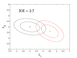
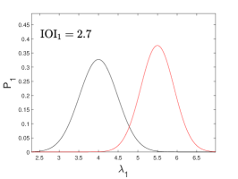
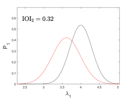
B.2 The analytic expression for the drop of IOI
In Sec. VI, we have defined the drop of IOI after marginalizing over (IOIk) as a supplemental measure of the one-parameter inconsistency in a multiparameter model. From the proof in Sec. B.1, especially from Eq. (90) and Eq. (89), we can obtain IOIk analytically and it is,
| (92) |
The above expression is not generically right, since it is not in an invariant form under a linear transformation along the axis. To generalize the result [Eq. (92)], we only need to find an invariant quantity that reduces to Eq. (92) in the case when takes the form of in Eq (86). We find that the general expression of IOIk is
| (93) |
where for . We have tested and verified that Eq. (93) is the same as the definition IOIk IOI IOImarg,k.
| Cases | Effect |
|---|---|
| Both IOIi and IOIi are small | Safe to marginalize over to analyze the inconsistency for the whole model |
| IOIi is small, but IOIi is large | Marginalization will hide the inconsistency due the correlation (specified by ) between and some other parameters |
| IOIi is small, but IOIi is large | Marginalization over will get a similar IOI as the whole model, but ignore the shape of the original probability distribution |
| Both IOIi and IOIi are large | Marginalization over will not be good for the analysis of the inconsistency |
B.3 A discussion on different situations in parameter marginalization
In general, the equality equation can be satisfied without or . An example is shown by the three panels in Fig. 12. It is a coincidence there for IOI to be the same after marginalizing over . The reason is as follows. If , we will have IOIIOI1 because marginalizing over hides some inconsistency due to the correlation between and specified by . In Fig. 12, , and the red ellipse is shifted a little downward compared to the case . As a result, the joint mean is located at a point which is more easily “supported” by the two experiments, and consequently IOI becomes smaller. Meanwhile, IOI1 does not depend on the vertical shift of both distributions. For a particular amount of vertical shift, IOI becomes the same as IOI1.
If the drop of IOI is small after parameter marginalization, we may be able to marginalize over the corresponding parameter to analyze the inconsistency for the whole model. If so, we can analyze the model in a low parameter dimension. And hopefully it can be reduced to two or three dimensions so that we can graphically show the full inconsistency. That is one of the motivations for us a we propose a supplemental measure of the inconsistency for one parameter (IOIi) in Sec. VI. However, even when the drop is small, we still need to pay attention to whether it is a special case such as the one shown in Fig. 12. In such a special case, marginalization over ignores the original probability distributions, although we get the same IOI. Fortunately, it is easy to check whether it is a special case. For example, if the drop of IOI after marginalizing over (i.e., IOI2) is small, we can check whether the IOI after marginalizing over all other parameters but (i.e., IOI2) is also small. If both IOI2 and IOI2 are small, we can safely marginalize over and analyze the inconsistency for the whole model. If not, marginalizing over will either hide some inconsistencies or ignore the original shape of the probability distribution. Table 12 summarizes the four situations regarding different combinations of IOIi and IOIi and the corresponding effects of marginalizing over the . In the right panel of Fig. 12, IOI2 is not so the example shown in Fig. 12 is a special case. Combining IOIi and IOIi, we can get a lot of information about the full distribution.
References
- Clifton et al. (2012) T. Clifton, P. G. Ferreira, A. Padilla, and C. Skordis, “Modified gravity and cosmology,” Phys. Rep. 513, 1–189 (2012), arXiv:1106.2476 .
- López-Corredoira (2017) M. López-Corredoira, “Tests and Problems of the Standard Model in Cosmology,” Foundations of Physics (2017), 10.1007/s10701-017-0073-8, arXiv:1701.08720 .
- Tsagas et al. (2008) C. G. Tsagas, A. Challinor, and R. Maartens, “Relativistic cosmology and large-scale structure,” Phys. Rep. 465, 61–147 (2008), arXiv:0705.4397 .
- Koyama (2016) K. Koyama, “Cosmological tests of modified gravity,” Reports on Progress in Physics 79, 046902 (2016), arXiv:1504.04623 .
- Joyce et al. (2015) A. Joyce, B. Jain, J. Khoury, and M. Trodden, “Beyond the cosmological standard model,” Phys. Rep. 568, 1–98 (2015), arXiv:1407.0059 .
- Ishak (2007) M. Ishak, “Remarks on the Formulation of the Cosmological Constant/Dark Energy Problems,” Foundations of Physics 37, 1470–1498 (2007), astro-ph/0504416 .
- Joyce et al. (2016) A. Joyce, L. Lombriser, and F. Schmidt, “Dark Energy Versus Modified Gravity,” Annual Review of Nuclear and Particle Science 66, 95–122 (2016), arXiv:1601.06133 .
- Bull et al. (2016) P. Bull et al., “Beyond CDM: Problems, solutions, and the road ahead,” Physics of the Dark Universe 12, 56–99 (2016), arXiv:1512.05356 .
- Debono and Smoot (2016) I. Debono and G. F. Smoot, “General Relativity and Cosmology: Unsolved Questions and Future Directions,” Universe 2, 23 (2016), arXiv:1609.09781 [gr-qc] .
- Ishak et al. (2006) M. Ishak, A. Upadhye, and D. N. Spergel, “Probing cosmic acceleration beyond the equation of state: Distinguishing between dark energy and modified gravity models,” Phys. Rev. D 74, 043513 (2006), astro-ph/0507184 .
- Wang et al. (2007) S. Wang, L. Hui, M. May, and Z. Haiman, “Is modified gravity required by observations? An empirical consistency test of dark energy models,” Phys. Rev. D 76, 063503 (2007), arXiv:0705.0165 .
- Ruiz and Huterer (2015) E. J. Ruiz and D. Huterer, “Testing the dark energy consistency with geometry and growth,” Phys. Rev. D 91, 063009 (2015), arXiv:1410.5832 .
- Bernal et al. (2016a) J. L. Bernal, L. Verde, and A. J. Cuesta, “Parameter splitting in dark energy: is dark energy the same in the background and in the cosmic structures?” J. Cosmol. Astropart. Phys. 2, 059 (2016a), arXiv:1511.03049 .
- Shafieloo (2012) A. Shafieloo, “Crossing statistic: Bayesian interpretation, model selection and resolving dark energy parametrization problem,” J. Cosmol. Astropart. Phys. 5, 024 (2012), arXiv:1202.4808 [astro-ph.CO] .
- Shafieloo and Hazra (2017) A. Shafieloo and D. K. Hazra, “Consistency of the Planck CMB data and CDM cosmology,” J. Cosmol. Astropart. Phys. 4, 012 (2017), arXiv:1610.07402 .
- Bernal et al. (2016b) J. L. Bernal, L. Verde, and A. G. Riess, “The trouble with H0,” J. Cosmol. Astropart. Phys. 10, 019 (2016b), arXiv:1607.05617 .
- Di Valentino et al. (2015) E. Di Valentino, A. Melchiorri, and J. Silk, “Beyond six parameters: Extending CDM,” Phys. Rev. D 92, 121302 (2015), arXiv:1507.06646 .
- Aubourg et al. (2015) É. Aubourg et al., “Cosmological implications of baryon acoustic oscillation measurements,” Phys. Rev. D 92, 123516 (2015), arXiv:1411.1074 .
- Heymans et al. (2013) C. Heymans et al., “CFHTLenS tomographic weak lensing cosmological parameter constraints: Mitigating the impact of intrinsic galaxy alignments,” Mon. Not. R. Astron. Soc. 432, 2433–2453 (2013), arXiv:1303.1808 .
- Charnock et al. (2017) T. Charnock, R. A. Battye, and A. Moss, “Planck data versus large scale structure: Methods to quantify discordance,” Phys. Rev. D 95, 123535 (2017), arXiv:1703.05959 .
- Betoule et al. (2014) M. Betoule et al., “Improved cosmological constraints from a joint analysis of the SDSS-II and SNLS supernova samples,” Astron. Astrophys. 568, A22 (2014), arXiv:1401.4064 .
- Beutler et al. (2011) F. Beutler, C. Blake, M. Colless, D. H. Jones, L. Staveley-Smith, L. Campbell, Q. Parker, W. Saunders, and F. Watson, “The 6dF Galaxy Survey: baryon acoustic oscillations and the local Hubble constant,” Mon. Not. R. Astron. Soc. 416, 3017–3032 (2011), arXiv:1106.3366 .
- Ade et al. (2016a) (Planck Collaboration) P. A. R. Ade et al. (Planck Collaboration), “Planck 2015 results. XIII. Cosmological parameters,” Astron. Astrophys. 594, A13 (2016a), arXiv:1502.01589 .
- Ade et al. (2016b) (Planck Collaboration) P. A. R. Ade et al. (Planck Collaboration), Astron. Astrophys. 594, A15 (2016b), arXiv:1502.01591 .
- Ade and others (2016) (Planck Collaboration) P. A. R. Ade and others (Planck Collaboration), “Planck 2015 results. XXIV. Cosmology from Sunyaev-Zeldovich cluster counts,” Astron. Astrophys. 594, A24 (2016), arXiv:1502.01597 .
- Blake et al. (2010) Chris Blake et al., “The WiggleZ Dark Energy Survey: the selection function and z = 0.6 galaxy power spectrum,” Mon. Not. R. Astron. Soc. 406, 803–821 (2010), arXiv:1003.5721 .
- Parkinson et al. (2012) David Parkinson, Signe Riemer-Sorensen, Chris Blake, Gregory B. Poole, Tamara M. Davis, et al., “The WiggleZ Dark Energy Survey: Final data release and cosmological results,” Phys. Rev. D 86, 103518 (2012), arXiv:1210.2130 .
- Alam et al. (2015) S. Alam et al., “The Eleventh and Twelfth Data Releases of the Sloan Digital Sky Survey: Final Data from SDSS-III,” Astrophys. J. Supp. 219, 12 (2015), arXiv:1501.00963 [astro-ph.IM] .
- Riess et al. (2016) A. G. Riess, L. M. Macri, S. L. Hoffmann, D. Scolnic, S. Casertano, A. V. Filippenko, B. E. Tucker, M. J. Reid, D. O. Jones, J. M. Silverman, R. Chornock, P. Challis, W. Yuan, P. J. Brown, and R. J. Foley, “A 2.4% Determination of the Local Value of the Hubble Constant,” Astrophys. J. 826, 56 (2016), arXiv:1604.01424 .
- Riess et al. (2011) A. G. Riess, L. Macri, S. Casertano, H. Lampeitl, H. C. Ferguson, A. V. Filippenko, S. W. Jha, W. Li, and R. Chornock, “A 3% Solution: Determination of the Hubble Constant with the Hubble Space Telescope and Wide Field Camera 3,” Astrophys. J. 730, 119 (2011), arXiv:1103.2976 .
- Adam and others (2016a) (Planck Collaboration) R. Adam and others (Planck Collaboration), “Planck intermediate results. XLVI. Reduction of large-scale systematic effects in HFI polarization maps and estimation of the reionization optical depth,” Astron. Astrophys. 596, A107 (2016a), arXiv:1605.02985 .
- Efstathiou (2014) G. Efstathiou, “H0 revisited,” Mon. Not. R. Astron. Soc. 440, 1138–1152 (2014), arXiv:1311.3461 .
- Casertano et al. (2017) S. Casertano, A. G. Riess, B. Bucciarelli, and M. G. Lattanzi, “A test of Gaia Data Release 1 parallaxes: implications for the local distance scale,” Astron. Astrophys. 599, A67 (2017), arXiv:1609.05175 [astro-ph.IM] .
- Bonvin et al. (2017) V. Bonvin et al., “H0LiCOW - V. New COSMOGRAIL time delays of HE 0435-1223: H0 to 3.8 per cent precision from strong lensing in a flat CDM model,” Mon. Not. R. Astron. Soc. 465, 4914–4930 (2017), arXiv:1607.01790 .
- Huang and Wang (2016) Q.-G. Huang and K. Wang, “How the dark energy can reconcile Planck with local determination of the Hubble constant,” European Physical Journal C 76, 506 (2016), arXiv:1606.05965 .
- Di Valentino et al. (2016a) E. Di Valentino, A. Melchiorri, and J. Silk, “Reconciling Planck with the local value of H0 in extended parameter space,” Physics Letters B 761, 242–246 (2016a), arXiv:1606.00634 .
- Hildebrandt et al. (2017) H. Hildebrandt et al., “KiDS-450: cosmological parameter constraints from tomographic weak gravitational lensing,” Mon. Not. R. Astron. Soc. 465, 1454–1498 (2017), arXiv:1606.05338 .
- Leauthaud et al. (2017) A. Leauthaud et al., “Lensing is low: cosmology, galaxy formation or new physics?” Mon. Not. R. Astron. Soc. 467, 3024–3047 (2017), arXiv:1611.08606 .
- Troxel and Ishak (2015) M. A. Troxel and M. Ishak, “The intrinsic alignment of galaxies and its impact on weak gravitational lensing in an era of precision cosmology,” Phys. Rep. 558, 1–59 (2015), arXiv:1407.6990 .
- Kirk et al. (2015) D. Kirk et al., “Galaxy Alignments: Observations and Impact on Cosmology,” Space Science Reviews 193, 139–211 (2015), arXiv:1504.05465 .
- Eifler et al. (2015) T. Eifler, E. Krause, S. Dodelson, A. R. Zentner, A. P. Hearin, and N. Y. Gnedin, “Accounting for baryonic effects in cosmic shear tomography: determining a minimal set of nuisance parameters using PCA,” Mon. Not. R. Astron. Soc. 454, 2451–2471 (2015), arXiv:1405.7423 .
- Dossett et al. (2015) J. N. Dossett, M. Ishak, D. Parkinson, and T. M. Davis, “Constraints and tensions in testing general relativity from Planck and CFHTLenS data including intrinsic alignment systematics,” Phys. Rev. D 92, 023003 (2015), arXiv:1501.03119 .
- Krause et al. (2016) E. Krause, T. Eifler, and J. Blazek, “The impact of intrinsic alignment on current and future cosmic shear surveys,” Mon. Not. R. Astron. Soc. 456, 207–222 (2016), arXiv:1506.08730 .
- Delubac et al. (2015) T. Delubac et al., “Baryon acoustic oscillations in the Ly forest of BOSS DR11 quasars,” Astron. Astrophys. 574, A59 (2015), arXiv:1404.1801 .
- Font-Ribera et al. (2014) A. Font-Ribera et al., “Quasar-Lyman forest cross-correlation from BOSS DR11: Baryon Acoustic Oscillations,” J. Cosmol. Astropart. Phys. 5, 027 (2014), arXiv:1311.1767 .
- Ferreira et al. (2017) Elisa G. M. Ferreira, Jerome Quintin, André A. Costa, E. Abdalla, and Bin Wang, “Evidence for interacting dark energy from boss,” Phys. Rev. D 95, 043520 (2017).
- Calabrese et al. (2008) E. Calabrese, A. Slosar, A. Melchiorri, G. F. Smoot, and O. Zahn, “Cosmic microwave weak lensing data as a test for the dark universe,” Phys. Rev. D 77, 123531 (2008), arXiv:0803.2309 .
- Di Valentino et al. (2016b) E. Di Valentino, A. Melchiorri, and J. Silk, “Cosmological hints of modified gravity?” Phys. Rev. D 93, 023513 (2016b), arXiv:1509.07501 .
- Muñoz et al. (2016) J. B. Muñoz, D. Grin, L. Dai, M. Kamionkowski, and E. D. Kovetz, “Search for compensated isocurvature perturbations with Planck power spectra,” Phys. Rev. D 93, 043008 (2016), arXiv:1511.04441 .
- Blake et al. (2011) C. Blake et al., “The WiggleZ Dark Energy Survey: the growth rate of cosmic structure since redshift z=0.9,” Mon. Not. R. Astron. Soc. 415, 2876–2891 (2011), arXiv:1104.2948 .
- Reid et al. (2014) B. A. Reid, H.-J. Seo, A. Leauthaud, J. L. Tinker, and M. White, “A 2.5 per cent measurement of the growth rate from small-scale redshift space clustering of SDSS-III CMASS galaxies,” Mon. Not. R. Astron. Soc. 444, 476–502 (2014), arXiv:1404.3742 .
- Vikhlinin et al. (2009) A. Vikhlinin et al., “Chandra Cluster Cosmology Project III: Cosmological Parameter Constraints,” Astrophys. J. 692, 1060–1074 (2009), arXiv:0812.2720 .
- Koyama (2006) K. Koyama, “Structure formation in modified gravity models,” J. Cosmol. Astropart. Phys. 3, 017 (2006), astro-ph/0601220 .
- Bertschinger (2006) E. Bertschinger, “On the Growth of Perturbations as a Test of Dark Energy and Gravity,” Astrophys. J. 648, 797–806 (2006), astro-ph/0604485 .
- Shapiro (2009) C. Shapiro, “Biased Dark Energy Constraints from Neglecting Reduced Shear in Weak-Lensing Surveys,” Astrophys. J. 696, 775–784 (2009), arXiv:0812.0769 .
- Jeffreys (1998) H. Jeffreys, The Theory of Probability, Oxford Classic Texts in the Physical Sciences (OUP Oxford, 1998).
- Verde et al. (2013) L. Verde, P. Protopapas, and R. Jimenez, “Planck and the local Universe: Quantifying the tension,” Physics of the Dark Universe 2, 166–175 (2013), arXiv:1306.6766 [astro-ph.CO] .
- Mortonson et al. (2010) M. J. Mortonson, D. Huterer, and W. Hu, “Figures of merit for present and future dark energy probes,” Phys. Rev. D 82, 063004 (2010), arXiv:1004.0236 .
- Lewis and Bridle (2002) A. Lewis and S. Bridle, “Cosmological parameters from CMB and other data: A Monte Carlo approach,” Phys. Rev. D 66, 103511 (2002), astro-ph/0205436 .
- Marshall et al. (2006) P. Marshall, N. Rajguru, and A. Slosar, “Bayesian evidence as a tool for comparing datasets,” Phys. Rev. D 73, 067302 (2006), astro-ph/0412535 .
- March et al. (2011) M. C. March, R. Trotta, L. Amendola, and D. Huterer, “Robustness to systematics for future dark energy probes,” Mon. Not. R. Astron. Soc. 415, 143–152 (2011), arXiv:1101.1521 .
- Amendola et al. (2013) L. Amendola, V. Marra, and M. Quartin, “Internal robustness: systematic search for systematic bias in SN Ia data,” Mon. Not. R. Astron. Soc. 430, 1867–1879 (2013), arXiv:1209.1897 [astro-ph.CO] .
- Seehars et al. (2016) S. Seehars, S. Grandis, A. Amara, and A. Refregier, “Quantifying concordance in cosmology,” Phys. Rev. D 93, 103507 (2016), arXiv:1510.08483 .
- MacCrann et al. (2015) N. MacCrann, J. Zuntz, S. Bridle, B. Jain, and M. R. Becker, “Cosmic discordance: are Planck CMB and CFHTLenS weak lensing measurements out of tune?” Mon. Not. R. Astron. Soc. 451, 2877–2888 (2015), arXiv:1408.4742 .
- Seehars et al. (2014) S. Seehars, A. Amara, A. Refregier, A. Paranjape, and J. Akeret, “Information gains from cosmic microwave background experiments,” Phys. Rev. D 90, 023533 (2014), arXiv:1402.3593 .
- Grandis et al. (2016a) S. Grandis, S. Seehars, A. Refregier, A. Amara, and A. Nicola, “Information gains from cosmological probes,” J. Cosmol. Astropart. Phys. 5, 034 (2016a), arXiv:1510.06422 .
- Zhao et al. (2017) G.-B. Zhao et al., “The clustering of galaxies in the completed SDSS-III Baryon Oscillation Spectroscopic Survey: Examining the observational evidence for dynamical dark energy,” ArXiv e-prints (2017), arXiv:1701.08165 .
- (68) S. Grandis and D. Rapetti (private communication).
- Grandis et al. (2016b) S. Grandis, D. Rapetti, A. Saro, J. J. Mohr, and J. P. Dietrich, “Quantifying tensions between CMB and distance data sets in models with free curvature or lensing amplitude,” Mon. Not. R. Astron. Soc. 463, 1416–1430 (2016b), arXiv:1604.06463 .
- Joudaki et al. (2017) S. Joudaki et al., “CFHTLenS revisited: assessing concordance with Planck including astrophysical systematics,” Mon. Not. R. Astron. Soc. 465, 2033–2052 (2017), arXiv:1601.05786 .
- Akaike (1974) H. Akaike, “A new look at the statistical model identification,” IEEE Transactions on Automatic Control 19, 716–723 (1974).
- Spiegelhalter et al. (2002) David J. Spiegelhalter, Nicola G. Best, Bradley P. Carlin, and Angelika Van Der Linde, “Bayesian measures of model complexity and fit,” Journal of the Royal Statistical Society: Series B (Statistical Methodology) 64, 583–639 (2002).
- Liddle (2007) A. R. Liddle, “Information criteria for astrophysical model selection,” Mon. Not. R. Astron. Soc. 377, L74–L78 (2007), astro-ph/0701113 .
- Ross et al. (2015) A. J. Ross, L. Samushia, C. Howlett, W. J. Percival, A. Burden, and M. Manera, “The clustering of the SDSS DR7 main Galaxy sample - I. A 4 per cent distance measure at z = 0.15,” Mon. Not. R. Astron. Soc. 449, 835–847 (2015), arXiv:1409.3242 .
- Adam and others (2016b) (Planck Collaboration) R. Adam and others (Planck Collaboration), “Planck intermediate results. XLVII. Planck constraints on reionization history,” Astron. Astrophys. 596, A108 (2016b), arXiv:1605.03507 .
- Di Valentino et al. (2017) E. Di Valentino, A. Melchiorri, E. V. Linder, and J. Silk, “Constraining dark energy dynamics in extended parameter space,” Phys. Rev. D 96, 023523 (2017), arXiv:1704.00762 .