Convergence analysis of a family of robust Kalman filters based on the contraction principlethanks: This work has been partially supported by the FIRB project “Learning meets time” (RBFR12M3AC) funded by MIUR.

Mattia Zorzi M. Zorzi is with the Dipartimento di Ingegneria dell’Informazione, Università di Padova, via Gradenigo 6/B, 35131 Padova, Italy, (email: zorzimat@dei.unipd.it).
Abstract

In this paper we analyze the convergence of a family of robust Kalman filters. For each filter of this family the model uncertainty is tuned according to the so called tolerance parameter. Assuming that the corresponding state-space model is reachable and observable, we show that the corresponding Riccati-like mapping is strictly contractive provided that the tolerance is sufficiently small, accordingly the filter converges.

keywords:
Block update, contraction mapping, Kalman filter, Riccati equation, Thompson’s part metric, risk-sensitive filtering
AMS:
60G35, 93B35, 93E11

1 Introduction

Robust Kalman filtering is a computational tool with widespread applications in many fields, e.g. [22]. In this paper we consider the parametric family of robust Kalman filters introduced in [28], see also the former works [17],[16],[9]. The parameter describing this family is denoted by τ𝜏\tau. Once τ𝜏\tau is fixed, the model uncertainty is represented by a ball which is about the nominal model and formed by placing a bound on the τ𝜏\tau-divergence, [27],[25],[26], between the actual and the nominal model. The bound is fixed by the user and represents the tolerance of the mismatch between the actual and the nominal model. Then, the robust filter is obtained by minimizing the mean square error according to the least favorable model in this ball. Interestingly, relaxing the assumption that the actual model belongs to the ball, we obtain a family of risk sensitive filters parametrized by τ𝜏\tau wherein the tolerance parameter is replaced by the so called risk sensitivity parameter. In particular, for τ=0𝜏0\tau=0 we obtain the usual risk sensitive filter, see [3, 19, 21, 12].

In this paper we analyze the convergence of this family of discrete-time robust Kalman filters. More precisely, we prove that the error covariance, obeying to a Riccati-like iteration, converges to a unique positive definite solution.

The convergence of Riccati-like iterations can be performed using classical argumentations, [6, 7, 5]. Alternatively, the convergence analysis can be performed using the contraction principle as in the former paper by Bougerol [4]. More precisely, under reachability and observability assumptions, he proved that the discrete-time Riccati iteration is a strict contraction for the Riemann metric associated to the cone of positive definite matrices. Interestingly, the same result holds using the Thompson’s part metric [15, 8]. The latter metric is more effective than the former in the sense that it gives a tighter bound on the convergence rate of the iteration. It is also worth noting that the contraction principle has been used also to prove the convergence of different kinds of nonlinear iterations [13, 14, 15].

The convergence analysis that we present here is based on the contraction principle. This analysis takes the root from the paper [18]. The latter studies the convergence of the risk sensitive Riccati iteration corresponding to the usual risk sensitive filter. In particular, placing an upper bound on the risk sensitivity parameter it is possible to prove that the N𝑁N-fold composition of the risk sensitive Riccati mapping is strictly contractive for the Thompson’s part metric. Since the robust Kalman filter with τ=0𝜏0\tau=0 can be understood as the usual risk sensitive filter where the risk sensitivity parameter is now time-varying, it is possible to characterize an upper bound on the tolerance of this robust filter in such a way that the time-varying risk sensitivity parameter is sufficiently small. In this way, the N𝑁N-fold composition of the mapping is strictly contractive and thus the robust filter converges, [29]. In this paper we extend these results for the entire family of robust Kalman filters.

The outline of the paper is as follows. In Section 2 we recall the Thompson’s part metric for positive definite matrices and the properties of contraction mappings. In Section 3 we review the robust Kalman filter, we derive the downsampled version and the corresponding N𝑁N-fold Riccati iteration. In this way we are able to derive a condition for which the iteration is strictly contractive. In Section 4 we translate this condition in terms of upper bound on the tolerance of the robust filter. In Section 5 an illustrative example is provided. In Section 6 deals with the convergence analysis of the family of τ𝜏\tau-risk sensitive filters. Finally, we draw the conclusions in Section 7.

Notation. Given xn𝑥superscript𝑛x\in\mathbb{R}^{n}, xnorm𝑥\|x\| denotes the Euclidean norm of x𝑥x, and xKsubscriptnorm𝑥𝐾\|x\|_{K} denotes the weighted Euclidean norm with weight matrix K𝐾K positive definite. The i𝑖i-th singular value of Pn×n𝑃superscript𝑛𝑛P\in\mathbb{R}^{n\times n} is denoted by σi(P)subscript𝜎𝑖𝑃\sigma_{i}(P) and σ1(P)σ2(P)σn(P)subscript𝜎1𝑃subscript𝜎2𝑃subscript𝜎𝑛𝑃\sigma_{1}(P)\geq\sigma_{2}(P)\geq\ldots\geq\sigma_{n}(P). Pnorm𝑃\|P\| denotes the spectral norm of P𝑃P, i.e. P=σ1(P)norm𝑃subscript𝜎1𝑃\|P\|=\sigma_{1}(P). 𝒬nsuperscript𝒬𝑛\mathcal{Q}^{n} denotes the vector space of symmetric matrices of dimension n×n𝑛𝑛n\times n. The cone of positive definite matrices in 𝒬nsuperscript𝒬𝑛\mathcal{Q}^{n} is denoted by 𝒬+nsuperscriptsubscript𝒬𝑛\mathcal{Q}_{+}^{n}, and its closure by 𝒬¯+nsuperscriptsubscript¯𝒬𝑛\bar{\mathcal{Q}}_{+}^{n}. diag(d1dn)diagsubscript𝑑1subscript𝑑𝑛\mathop{\operator@font diag}\nolimits(d_{1}\ldots d_{n}) denotes the diagonal matrix with elements in the main diagonal d1,,dnsubscript𝑑1subscript𝑑𝑛d_{1},\ldots,d_{n}; similarly blkdiag(P1Pn)blkdiagsubscript𝑃1subscript𝑃𝑛\mathrm{blkdiag}(P_{1}\ldots P_{n}) denotes the block-diagonal matrix with matrices in the main block-diagonal P1,,Pnsubscript𝑃1subscript𝑃𝑛P_{1},\ldots,P_{n}. Given P𝒬+n𝑃superscriptsubscript𝒬𝑛P\in\mathcal{Q}_{+}^{n} with eigendecomposition P=UDUT𝑃𝑈𝐷superscript𝑈𝑇P=UDU^{T} such that U𝑈U is an orthogonal matrix and D=diag(σ1(P)σn(P))𝐷diagsubscript𝜎1𝑃subscript𝜎𝑛𝑃D=\mathop{\operator@font diag}\nolimits(\sigma_{1}(P)\ldots\sigma_{n}(P)), the exponentiation of P𝑃P to a real number τ𝜏\tau is defined as Pτ=UDτUTsuperscript𝑃𝜏𝑈superscript𝐷𝜏superscript𝑈𝑇P^{\tau}=UD^{\tau}U^{T} with Dτ=diag(σ1(P)τσn(P)τ)superscript𝐷𝜏diagsubscript𝜎1superscript𝑃𝜏subscript𝜎𝑛superscript𝑃𝜏D^{\tau}=\mathop{\operator@font diag}\nolimits(\sigma_{1}(P)^{\tau}\ldots\sigma_{n}(P)^{\tau}). Similarly, we define exp(P)=Uexp(D)UT𝑃𝑈𝐷superscript𝑈𝑇\exp(P)=U\exp(D)U^{T} with exp(D)=diag(eσ1(P)eσn(P))𝐷diagsuperscript𝑒subscript𝜎1𝑃superscript𝑒subscript𝜎𝑛𝑃\exp(D)=\mathop{\operator@font diag}\nolimits(e^{\sigma_{1}(P)}\ldots e^{\sigma_{n}(P)}) and log(P)=Ulog(D)UT𝑃𝑈𝐷superscript𝑈𝑇\log(P)=U\log(D)U^{T} with log(D)=diag(log(σ1(P))log(σn(P)))𝐷diagsubscript𝜎1𝑃subscript𝜎𝑛𝑃\log(D)=\mathop{\operator@font diag}\nolimits(\log(\sigma_{1}(P))\ldots\log(\sigma_{n}(P))).

2 Thompson’s part metric and contraction mappings

Let P𝑃P and Q𝑄Q belong to 𝒬+nsuperscriptsubscript𝒬𝑛\mathcal{Q}_{+}^{n}. The Thompson’s part metric [2] between P𝑃P and Q𝑄Q is defined as

dT(P,Q)subscript𝑑𝑇𝑃𝑄\displaystyle d_{T}(P,Q) =log(P1/2QP1/2)absentnormsuperscript𝑃12𝑄superscript𝑃12\displaystyle=\|\log(P^{-1/2}QP^{-1/2})\|
=max{log(σ1(P1Q)),log(σ1(Q1P))}.absentsubscript𝜎1superscript𝑃1𝑄subscript𝜎1superscript𝑄1𝑃\displaystyle=\max\{\log(\sigma_{1}(P^{-1}Q)),\log(\sigma_{1}(Q^{-1}P))\}.

Beside all the traditional properties of a distance, dTsubscript𝑑𝑇d_{T} has the feature that it is invariant under matrix inversion and congruence transformations.

Let h()h(\cdot) be an arbitrary mapping in 𝒬+nsuperscriptsubscript𝒬𝑛\mathcal{Q}_{+}^{n}. We say that hh is strictly contractive if its contraction coefficient (or Lipschitz constant)

ξ(h)=supP,Q𝒬n+,PQdT(h(P),h(Q))dT(P,Q)𝜉subscriptsupremumformulae-sequence𝑃𝑄superscriptsubscript𝒬𝑛𝑃𝑄subscript𝑑𝑇𝑃𝑄subscript𝑑𝑇𝑃𝑄\displaystyle\xi(h)=\sup_{P,Q\in\mathcal{Q}_{n}^{+},P\neq Q}\frac{d_{T}(h(P),h(Q))}{d_{T}(P,Q)}

is less than one. Since the metric space (𝒬+n,dT)superscriptsubscript𝒬𝑛subscript𝑑𝑇(\mathcal{Q}_{+}^{n},d_{T}) is complete [20], if hh is a strict contraction of 𝒬+nsuperscriptsubscript𝒬𝑛\mathcal{Q}_{+}^{n} for the distance dTsubscript𝑑𝑇d_{T}, by the Banach fixed point theorem, [1, p. 244], there exists a unique fixed point P𝑃P of hh in 𝒬+nsuperscriptsubscript𝒬𝑛\mathcal{Q}_{+}^{n} satisfying P=h(P)𝑃𝑃P=h(P). Moreover, this fixed point is given by performing the iteration Pk+1=h(Pk)subscript𝑃𝑘1subscript𝑃𝑘P_{k+1}=h(P_{k}) starting with any P0𝒬+nsubscript𝑃0superscriptsubscript𝒬𝑛P_{0}\in\mathcal{Q}_{+}^{n}. Consider the downsampled iteration Pk+1d=hkN(Pkd)superscriptsubscript𝑃𝑘1𝑑superscriptsubscript𝑘𝑁superscriptsubscript𝑃𝑘𝑑P_{k+1}^{d}=h_{k}^{N}(P_{k}^{d}) where Pkd=PkNsuperscriptsubscript𝑃𝑘𝑑subscript𝑃𝑘𝑁P_{k}^{d}=P_{kN} and N𝑁N is an integer. Here, hkNsuperscriptsubscript𝑘𝑁h_{k}^{N} is the N𝑁N-fold composition of hh at step kN𝑘𝑁kN. If hkNsuperscriptsubscript𝑘𝑁h_{k}^{N} is strictly contractive for kq~𝑘~𝑞k\geq\tilde{q} with q~~𝑞\tilde{q} fixed, then hh has a unique fixed point given as before. In this paper we will need the next Lemma [15, Th. 5.3].

Lemma 2.1.

Let W1,W2𝒬+nsubscript𝑊1subscript𝑊2superscriptsubscript𝒬𝑛W_{1},W_{2}\in\mathcal{Q}_{+}^{n}. Then, the mapping

h(P)=M(P1+W1)1MT+W2𝑃𝑀superscriptsuperscript𝑃1subscript𝑊11superscript𝑀𝑇subscript𝑊2\displaystyle h(P)=M(P^{-1}+W_{1})^{-1}M^{T}+W_{2}

is strictly contractive with

ξ(h)(σ1(W11MTW21M)1+1+σ1(W11MTW21M))2.𝜉superscriptsubscript𝜎1superscriptsubscript𝑊11superscript𝑀𝑇superscriptsubscript𝑊21𝑀11subscript𝜎1superscriptsubscript𝑊11superscript𝑀𝑇superscriptsubscript𝑊21𝑀2\displaystyle\xi(h)\leq\left(\frac{\sqrt{\sigma_{1}(W_{1}^{-1}M^{T}W_{2}^{-1}M)}}{1+\sqrt{1+\sigma_{1}(W_{1}^{-1}M^{T}W_{2}^{-1}M)}}\right)^{2}.

It is worth noting that the results outlined in this Section also hold using the Riemann metric [4]. On the other hand, the Thompson’s part metric is more effective than the Riemann one because it provides a tighter bound on the convergence rate of the previous iteration.

3 Contraction property of the robust Kalman filters

Consider the state-space model

xk+1subscript𝑥𝑘1\displaystyle x_{k+1} =Axk+Bvkabsent𝐴subscript𝑥𝑘𝐵subscript𝑣𝑘\displaystyle=Ax_{k}+Bv_{k}
yksubscript𝑦𝑘\displaystyle y_{k} =Cxk+Dvkabsent𝐶subscript𝑥𝑘𝐷subscript𝑣𝑘\displaystyle=Cx_{k}+Dv_{k} (1)

where xknsubscript𝑥𝑘superscript𝑛x_{k}\in\mathbb{R}^{n} is the state process, ykpsubscript𝑦𝑘superscript𝑝y_{k}\in\mathbb{R}^{p} is the observation process and vkmsubscript𝑣𝑘superscript𝑚v_{k}\in\mathbb{R}^{m} is white Gaussian noise with unit variance, i.e. 𝔼[vkvkT]=Im𝔼delimited-[]subscript𝑣𝑘superscriptsubscript𝑣𝑘𝑇subscript𝐼𝑚\mathbb{E}[v_{k}v_{k}^{T}]=I_{m}. The initial state x0subscript𝑥0x_{0} is assumed to be independent of vksubscript𝑣𝑘v_{k}. Moreover, its nominal probability density is f0(x0)𝒩(x^0,V0)similar-tosubscript𝑓0subscript𝑥0𝒩subscript^𝑥0subscript𝑉0f_{0}(x_{0})\sim\mathcal{N}(\hat{x}_{0},V_{0}). Model (3) is completely described by the nominal joint Gaussian probability density fk(xk+1,yk|Yk1)subscript𝑓𝑘subscript𝑥𝑘1conditionalsubscript𝑦𝑘subscript𝑌𝑘1f_{k}(x_{k+1},y_{k}|Y_{k-1}) of xk+1subscript𝑥𝑘1x_{k+1} and yksubscript𝑦𝑘y_{k} conditioned on Yk1:=[y0yk1]Tassignsubscript𝑌𝑘1superscriptdelimited-[]subscript𝑦0subscript𝑦𝑘1𝑇Y_{k-1}:=[\,y_{0}\,\ldots y_{k-1}\,]^{T}. We consider the family of robust Kalman filters [28],[17] parametrized by τ[0,1]𝜏01\tau\in[0,1]:

x^k+1=argmingk𝒢kmaxf~kk,τc𝔼f~k[xk+1gk(yk)2|Yk1]subscript^𝑥𝑘1subscript𝑔𝑘subscript𝒢𝑘argminsubscript~𝑓𝑘subscriptsuperscript𝑐𝑘𝜏subscript𝔼subscript~𝑓𝑘delimited-[]conditionalsuperscriptnormsubscript𝑥𝑘1subscript𝑔𝑘subscript𝑦𝑘2subscript𝑌𝑘1\displaystyle\hat{x}_{k+1}=\underset{g_{k}\in\mathcal{G}_{k}}{\mathrm{argmin}}\underset{\tilde{f}_{k}\in\mathcal{B}^{c}_{k,\tau}}{\max}\mathbb{E}_{\tilde{f}_{k}}[\|x_{k+1}-g_{k}(y_{k})\|^{2}|Y_{k-1}]

where 𝔼f~k[|Yk1]\mathbb{E}_{\tilde{f}_{k}}[\cdot|Y_{k-1}] is the conditional expectation taken with respect to f~k(xk+1,yk|Yk1)subscript~𝑓𝑘subscript𝑥𝑘1conditionalsubscript𝑦𝑘subscript𝑌𝑘1\tilde{f}_{k}(x_{k+1},y_{k}|Y_{k-1}) which is the least-favorable joint Gaussian probability density of xk+1subscript𝑥𝑘1x_{k+1} and yksubscript𝑦𝑘y_{k} conditioned on Yk1subscript𝑌𝑘1Y_{k-1}. k,τcsubscriptsuperscript𝑐𝑘𝜏\mathcal{B}^{c}_{k,\tau} is a ball about the nominal density fk(xk+1,yk|Yk1)subscript𝑓𝑘subscript𝑥𝑘1conditionalsubscript𝑦𝑘subscript𝑌𝑘1f_{k}(x_{k+1},y_{k}|Y_{k-1}) with radius c𝑐c:

k,τc={f~k(zk|Yk1) s.t. 𝒟τ(f~kfk)c}subscriptsuperscript𝑐𝑘𝜏subscript~𝑓𝑘conditionalsubscript𝑧𝑘subscript𝑌𝑘1 s.t. subscript𝒟𝜏conditionalsubscript~𝑓𝑘subscript𝑓𝑘𝑐\displaystyle\mathcal{B}^{c}_{k,\tau}=\{\tilde{f}_{k}(z_{k}|Y_{k-1})\hbox{ s.t. }\mathcal{D}_{\tau}(\tilde{f}_{k}\|f_{k})\leq c\}

where 𝒟τsubscript𝒟𝜏\mathcal{D}_{\tau} is the τ𝜏\tau-divergence family with parameter τ[0,1]𝜏01\tau\in[0,1] and defined as follows. Let f~~𝑓\tilde{f} and f𝑓f be two q𝑞q-dimensional Gaussian probability densities with mean vector m~z,mzsubscript~𝑚𝑧subscript𝑚𝑧\tilde{m}_{z},m_{z} and covariance matrix K~z,Kzsubscript~𝐾𝑧subscript𝐾𝑧\tilde{K}_{z},K_{z}, respectively. Then, the τ𝜏\tau-divergence family is defined as

𝒟τsubscript𝒟𝜏\displaystyle\mathcal{D}_{\tau} (f~f)=conditional~𝑓𝑓absent\displaystyle(\tilde{f}\|f)=
{ΔmzKZ12+tr(log(K~zKz1)+K~zKz1Iq),τ=011τΔmzKZ12+tr(1τ(τ1)(Lz1K~zLzT)τ+11τK~zKz1+1τIq),0<τ<1δ(Δmz)+tr(Lz1K~zLzTlog(Lz1K~zLzT)K~zKz1+Iq),τ=1 casessubscriptsuperscriptnormΔsubscript𝑚𝑧2superscriptsubscript𝐾𝑍1trsubscript~𝐾𝑧superscriptsubscript𝐾𝑧1subscript~𝐾𝑧superscriptsubscript𝐾𝑧1subscript𝐼𝑞𝜏011𝜏subscriptsuperscriptnormΔsubscript𝑚𝑧2superscriptsubscript𝐾𝑍1tr1𝜏𝜏1superscriptsuperscriptsubscript𝐿𝑧1subscript~𝐾𝑧superscriptsubscript𝐿𝑧𝑇𝜏11𝜏subscript~𝐾𝑧superscriptsubscript𝐾𝑧11𝜏subscript𝐼𝑞0𝜏1𝛿Δsubscript𝑚𝑧trsuperscriptsubscript𝐿𝑧1subscript~𝐾𝑧superscriptsubscript𝐿𝑧𝑇superscriptsubscript𝐿𝑧1subscript~𝐾𝑧superscriptsubscript𝐿𝑧𝑇subscript~𝐾𝑧superscriptsubscript𝐾𝑧1subscript𝐼𝑞τ=1 \displaystyle\left\{\begin{array}[]{ll}\|\Delta m_{z}\|^{2}_{K_{Z}^{-1}}+\mathop{\rm tr}\left(-\log(\tilde{K}_{z}K_{z}^{-1})+\tilde{K}_{z}K_{z}^{-1}-I_{q}\right),&\hbox{$\tau=0$}\\ \frac{1}{1-\tau}\|\Delta m_{z}\|^{2}_{K_{Z}^{-1}}+\mathop{\rm tr}\left(\frac{1}{\tau(\tau-1)}(L_{z}^{-1}\tilde{K}_{z}L_{z}^{-T})^{\tau}+\frac{1}{1-\tau}\tilde{K}_{z}K_{z}^{-1}+\frac{1}{\tau}I_{q}\right),&\hbox{$0<\tau<1$}\\ \delta(\Delta m_{z})+\mathop{\rm tr}\left(L_{z}^{-1}\tilde{K}_{z}L_{z}^{-T}\log(L_{z}^{-1}\tilde{K}_{z}L_{z}^{-T})-\tilde{K}_{z}K_{z}^{-1}+I_{q}\right),&\hbox{$\tau=1$ }\end{array}\right. (5)

where Δmz=mzm~zΔsubscript𝑚𝑧subscript𝑚𝑧subscript~𝑚𝑧\Delta m_{z}=m_{z}-\tilde{m}_{z} and Lzsubscript𝐿𝑧L_{z} is such that Kz=LzLzTsubscript𝐾𝑧subscript𝐿𝑧subscriptsuperscript𝐿𝑇𝑧K_{z}=L_{z}L^{T}_{z}. Note that, 𝒟τ(f~f)subscript𝒟𝜏conditional~𝑓𝑓\mathcal{D}_{\tau}(\tilde{f}\|f) coincides with the Kullback-Leibler divergence for τ=0𝜏0\tau=0, [24]. To understand the role of parameter τ𝜏\tau in k,τcsuperscriptsubscript𝑘𝜏𝑐\mathcal{B}_{k,\tau}^{c} consider the ball τc:={f~:𝒟τ(f~f)c}assignsuperscriptsubscript𝜏𝑐conditional-set~𝑓subscript𝒟𝜏conditional~𝑓𝑓𝑐\mathcal{B}_{\tau}^{c}:=\{\tilde{f}\,:\,\mathcal{D}_{\tau}(\tilde{f}\|f)\leq c\}. In [27], it has been shown that, increasing τ𝜏\tau and choosing c𝑐c in such a way that the measure of τcsuperscriptsubscript𝜏𝑐\mathcal{B}_{\tau}^{c} remains constant, then the uncertainty described by τcsuperscriptsubscript𝜏𝑐\mathcal{B}_{\tau}^{c} increases for the covariance matrix while it decreases for the mean vector. Accordingly, τ𝜏\tau tunes how to allocate the mismodeling budget between the mean vector and the covariance matrix. c𝑐c is referred to as tolerance and measures the model uncertainty. 𝒢ksubscript𝒢𝑘\mathcal{G}_{k} is the class of estimators with finite second-order moments with respect to all densities f~k(xk+1,yk|Yk1)k,τcsubscript~𝑓𝑘subscript𝑥𝑘1conditionalsubscript𝑦𝑘subscript𝑌𝑘1subscriptsuperscript𝑐𝑘𝜏\tilde{f}_{k}(x_{k+1},y_{k}|Y_{k-1})\in\mathcal{B}^{c}_{k,\tau}. The resulting estimator obeys the recursion:

x^k+1=Ax^k+Gk(ykCx^k)subscript^𝑥𝑘1𝐴subscript^𝑥𝑘subscript𝐺𝑘subscript𝑦𝑘𝐶subscript^𝑥𝑘\displaystyle\hat{x}_{k+1}=A\hat{x}_{k}+G_{k}(y_{k}-C\hat{x}_{k}) (6)

where Gksubscript𝐺𝑘G_{k} is the gain matrix

Gksubscript𝐺𝑘\displaystyle G_{k} =(AVkCT+BDT)(CVkCT+DDT)1.absent𝐴subscript𝑉𝑘superscript𝐶𝑇𝐵superscript𝐷𝑇superscript𝐶subscript𝑉𝑘superscript𝐶𝑇𝐷superscript𝐷𝑇1\displaystyle=(AV_{k}C^{T}+BD^{T})(CV_{k}C^{T}+DD^{T})^{-1}. (7)

If xkx^ksubscript𝑥𝑘subscript^𝑥𝑘x_{k}-\hat{x}_{k} denotes the state prediction error at time k𝑘k, its pseudo-nominal and least-favorable covariance matrix is denoted by Pksubscript𝑃𝑘P_{k} and Vksubscript𝑉𝑘V_{k}, respectively. Then, the latter obey to the Riccati-like iteration:

Pk+1subscript𝑃𝑘1\displaystyle P_{k+1} =AVkATGk(CVkCT+DDT)GkT+BBTabsent𝐴subscript𝑉𝑘superscript𝐴𝑇subscript𝐺𝑘𝐶subscript𝑉𝑘superscript𝐶𝑇𝐷superscript𝐷𝑇superscriptsubscript𝐺𝑘𝑇𝐵superscript𝐵𝑇\displaystyle=AV_{k}A^{T}-G_{k}(CV_{k}C^{T}+DD^{T})G_{k}^{T}+BB^{T} (8)
Vk+1subscript𝑉𝑘1\displaystyle V_{k+1} ={LPk+1(Inθk(1τ)LPk+1TLPk+1)1τ1LPk+1T,0τ<1LPk+1exp(θkLPk+1TLPk+1)LPk+1T,τ=1absentcasessubscript𝐿subscript𝑃𝑘1superscriptsubscript𝐼𝑛subscript𝜃𝑘1𝜏superscriptsubscript𝐿subscript𝑃𝑘1𝑇subscript𝐿subscript𝑃𝑘11𝜏1superscriptsubscript𝐿subscript𝑃𝑘1𝑇0𝜏1subscript𝐿subscript𝑃𝑘1subscript𝜃𝑘superscriptsubscript𝐿subscript𝑃𝑘1𝑇subscript𝐿subscript𝑃𝑘1superscriptsubscript𝐿subscript𝑃𝑘1𝑇𝜏1\displaystyle=\left\{\begin{array}[]{ll}L_{P_{k+1}}\left(I_{n}-\theta_{k}(1-\tau)L_{P_{k+1}}^{T}L_{P_{k+1}}\right)^{\frac{1}{\tau-1}}L_{P_{k+1}}^{T},&0\leq\tau<1\\ L_{P_{k+1}}\exp\left(\theta_{k}L_{P_{k+1}}^{T}L_{P_{k+1}}\right)L_{P_{k+1}}^{T},&\tau=1\end{array}\right. (11)

where LPk+1subscript𝐿subscript𝑃𝑘1L_{P_{k+1}} is such that Pk+1=LPk+1LPk+1Tsubscript𝑃𝑘1subscript𝐿subscript𝑃𝑘1superscriptsubscript𝐿subscript𝑃𝑘1𝑇P_{k+1}=L_{P_{k+1}}L_{P_{k+1}}^{T} and θk1>(1τ)Pk+1superscriptsubscript𝜃𝑘11𝜏normsubscript𝑃𝑘1\theta_{k}^{-1}>(1-\tau)\|P_{k+1}\| is the unique solution to

c=γτ(Pk+1,θk)𝑐subscript𝛾𝜏subscript𝑃𝑘1subscript𝜃𝑘\displaystyle c=\gamma_{\tau}(P_{k+1},\theta_{k}) (12)

where γτsubscript𝛾𝜏\gamma_{\tau} is defined as:

γτ(P,θ)={logdet(InθP)1+tr((InθP)1In),τ=0tr(1τ(1τ)(Inθ(1τ)LPTLP)ττ1+11τ(Inθ(1τ)LPTLP)1τ1+1τIn),0<τ<1tr(exp(θLPTLP)(θLPTLPIn)+In),τ=1.\displaystyle\gamma_{\tau}(P,\theta)=\left\{\begin{array}[]{ll}-\log\det(I_{n}-\theta P)^{-1}+\mathop{\rm tr}((I_{n}-\theta P)^{-1}-I_{n}),&\tau=0\\ \mathop{\rm tr}(-\frac{1}{\tau(1-\tau)}(I_{n}-\theta(1-\tau)L_{P}^{T}L_{P})^{\frac{\tau}{\tau-1}}\\ \hskip 8.5359pt+\frac{1}{1-\tau}(I_{n}-\theta(1-\tau)L_{P}^{T}L_{P})^{\frac{1}{\tau-1}}+\frac{1}{\tau}I_{n}),&0<\tau<1\\ \mathop{\rm tr}(\exp(\theta L_{P}^{T}L_{P})(\theta L_{P}^{T}L_{P}-I_{n})+I_{n}),&\tau=1.\end{array}\right. (17)

θksubscript𝜃𝑘\theta_{k} is called risk sensitivity parameter and it is time-varying. In the case that c=0𝑐0c=0, i.e. no uncertainty in the nominal model, we obtain the usual Kalman filter. Regarding the performance analysis of this family of robust Kalman filters with respect to parameter τ𝜏\tau we refer to [28]. It is worth noting, in view of (11), we have that Pk+1<Vk+1subscript𝑃𝑘1subscript𝑉𝑘1P_{k+1}<V_{k+1}. To study the asymptotic behavior of this robust Kalman filter, the matrices A𝐴A, B𝐵B, C𝐶C, D𝐷D and the tolerance c𝑐c are assumed to be constant. Without loss of generality we assume that BDT=0𝐵superscript𝐷𝑇0BD^{T}=0. Otherwise, we can rewrite the filter (6)-(17) with A~=ABDT(DDT)1C~𝐴𝐴𝐵superscript𝐷𝑇superscript𝐷superscript𝐷𝑇1𝐶\tilde{A}=A-BD^{T}(DD^{T})^{-1}C, B~~𝐵\tilde{B} such that B~B~T=B(IDT(DDT)1D)BT~𝐵superscript~𝐵𝑇𝐵𝐼superscript𝐷𝑇superscript𝐷superscript𝐷𝑇1𝐷superscript𝐵𝑇\tilde{B}\tilde{B}^{T}=B(I-D^{T}(DD^{T})^{-1}D)B^{T}, C~=C~𝐶𝐶\tilde{C}=C and D~=D~𝐷𝐷\tilde{D}=D. In this way B~D~T=0~𝐵superscript~𝐷𝑇0\tilde{B}\tilde{D}^{T}=0. Substituting (7) in (8) and using the Woodbury formula, we obtain the Riccati-like iteration

Pk+1=rτ,c(Pk):=A(Vk1+CT(DDT)1C)1AT+BBT.subscript𝑃𝑘1subscript𝑟𝜏𝑐subscript𝑃𝑘assign𝐴superscriptsuperscriptsubscript𝑉𝑘1superscript𝐶𝑇superscript𝐷superscript𝐷𝑇1𝐶1superscript𝐴𝑇𝐵superscript𝐵𝑇\displaystyle P_{k+1}=r_{\tau,c}(P_{k}):=A(V_{k}^{-1}+C^{T}(DD^{T})^{-1}C)^{-1}A^{T}+BB^{T}. (18)

Defining the positive definite matrix

Φk=Pk+11Vk+11subscriptΦ𝑘superscriptsubscript𝑃𝑘11superscriptsubscript𝑉𝑘11\displaystyle\Phi_{k}=P_{k+1}^{-1}-V_{k+1}^{-1}

we have

rτ,c(Pk)subscript𝑟𝜏𝑐subscript𝑃𝑘\displaystyle r_{\tau,c}(P_{k}) =A(Pk1Φk1+CT(DDT)1C)1AT+BBT.absent𝐴superscriptsuperscriptsubscript𝑃𝑘1subscriptΦ𝑘1superscript𝐶𝑇superscript𝐷superscript𝐷𝑇1𝐶1superscript𝐴𝑇𝐵superscript𝐵𝑇\displaystyle=A(P_{k}^{-1}-\Phi_{k-1}+C^{T}(DD^{T})^{-1}C)^{-1}A^{T}+BB^{T}. (19)

The mapping in (19) has the same structure of the risk sensitive Riccati mapping, [21]. Accordingly, the robust filter (6)-(17) can be interpreted as solving a standard least-square filtering problem with time-varying parameters in Krein space, [10, 11]. The Krein state-space model consists of dynamics and observations in (3), to which we must adjoin the new observations 0=xk+uk0subscript𝑥𝑘subscript𝑢𝑘0=x_{k}+u_{k}. The components of noise vectors vksubscript𝑣𝑘v_{k} and uksubscript𝑢𝑘u_{k} now belong to a Krein space and have the inner product

[vkuk],[vsus]=[Im00Φk11]δksdelimited-[]subscript𝑣𝑘subscript𝑢𝑘delimited-[]subscript𝑣𝑠subscript𝑢𝑠delimited-[]subscript𝐼𝑚00superscriptsubscriptΦ𝑘11subscript𝛿𝑘𝑠\displaystyle\left\langle\left[\begin{array}[]{c}v_{k}\\ u_{k}\end{array}\right]\,,\,\left[\begin{array}[]{c}v_{s}\\ u_{s}\end{array}\right]\right\rangle=\left[\begin{array}[]{cc}I_{m}&0\\ 0&-\Phi_{k-1}^{-1}\\ \end{array}\right]\delta_{k-s} (26)

where δksubscript𝛿𝑘\delta_{k} denotes the Kronecker delta function. Since xksubscript𝑥𝑘x_{k} is Gauss-Markov, the downsampled process xkd:=xkNassignsuperscriptsubscript𝑥𝑘𝑑subscript𝑥𝑘𝑁x_{k}^{d}:=x_{kN}, with N𝑁N integer, is also Gauss-Markov with state-space model

xk+1dsuperscriptsubscript𝑥𝑘1𝑑\displaystyle x_{k+1}^{d} =ANxkd+N𝐯kNabsentsuperscript𝐴𝑁superscriptsubscript𝑥𝑘𝑑subscript𝑁superscriptsubscript𝐯𝑘𝑁\displaystyle=A^{N}x_{k}^{d}+{\cal R}_{N}{\bf v}_{k}^{N}
𝐲kNsuperscriptsubscript𝐲𝑘𝑁\displaystyle{\bf y}_{k}^{N} =𝒪Nxkd+𝒟N𝐯kN+N𝐯kNabsentsubscript𝒪𝑁superscriptsubscript𝑥𝑘𝑑subscript𝒟𝑁superscriptsubscript𝐯𝑘𝑁subscript𝑁superscriptsubscript𝐯𝑘𝑁\displaystyle={\cal O}_{N}x_{k}^{d}+{\cal D}_{N}{\bf v}_{k}^{N}+{\cal H}_{N}{\bf v}_{k}^{N}
𝟎0\displaystyle{\bf 0} =𝒪NRxkd+𝐮kN+N𝐯kNabsentsuperscriptsubscript𝒪𝑁𝑅superscriptsubscript𝑥𝑘𝑑superscriptsubscript𝐮𝑘𝑁subscript𝑁superscriptsubscript𝐯𝑘𝑁\displaystyle={\cal O}_{N}^{R}x_{k}^{d}+{\bf u}_{k}^{N}+{\cal L}_{N}{\bf v}_{k}^{N} (27)

where

𝐯kNsuperscriptsubscript𝐯𝑘𝑁\displaystyle{\bf v}_{k}^{N} =[vkN+N1TvkN+N2TvkNT]Tabsentsuperscriptdelimited-[]superscriptsubscript𝑣𝑘𝑁𝑁1𝑇superscriptsubscript𝑣𝑘𝑁𝑁2𝑇superscriptsubscript𝑣𝑘𝑁𝑇𝑇\displaystyle=\left[\begin{array}[]{cccc}v_{kN+N-1}^{T}&v_{kN+N-2}^{T}&\ldots&v_{kN}^{T}\end{array}\right]^{T} (29)
𝐮kNsuperscriptsubscript𝐮𝑘𝑁\displaystyle{\bf u}_{k}^{N} =[ukN+N1TukN+N2TukNT]Tabsentsuperscriptdelimited-[]superscriptsubscript𝑢𝑘𝑁𝑁1𝑇superscriptsubscript𝑢𝑘𝑁𝑁2𝑇superscriptsubscript𝑢𝑘𝑁𝑇𝑇\displaystyle=\left[\begin{array}[]{cccc}u_{kN+N-1}^{T}&u_{kN+N-2}^{T}&\ldots&u_{kN}^{T}\end{array}\right]^{T} (31)
𝐲kNsuperscriptsubscript𝐲𝑘𝑁\displaystyle{\bf y}_{k}^{N} =[ykN+N1TykN+N2TykNT]T.absentsuperscriptdelimited-[]superscriptsubscript𝑦𝑘𝑁𝑁1𝑇superscriptsubscript𝑦𝑘𝑁𝑁2𝑇superscriptsubscript𝑦𝑘𝑁𝑇𝑇\displaystyle=\left[\begin{array}[]{cccc}y_{kN+N-1}^{T}&y_{kN+N-2}^{T}&\ldots&y_{kN}^{T}\end{array}\right]^{T}. (33)

In model (27) we have

Nsubscript𝑁\displaystyle{\cal R}_{N} =[BABAN1B]absentdelimited-[]𝐵𝐴𝐵superscript𝐴𝑁1𝐵\displaystyle=\left[\begin{array}[]{cccc}B&AB&\ldots&A^{N-1}B\end{array}\right] (35)
𝒪Nsubscript𝒪𝑁\displaystyle{\cal O}_{N} =[(CAN1)T(CA)TCT]Tabsentsuperscriptdelimited-[]superscript𝐶superscript𝐴𝑁1𝑇superscript𝐶𝐴𝑇superscript𝐶𝑇𝑇\displaystyle=\left[\begin{array}[]{cccc}(CA^{N-1})^{T}&\ldots&(CA)^{T}&C^{T}\end{array}\right]^{T} (37)
𝒪NRsuperscriptsubscript𝒪𝑁𝑅\displaystyle{\cal O}_{N}^{R} =[(AN1)T(A)TI]Tabsentsuperscriptdelimited-[]superscriptsuperscript𝐴𝑁1𝑇superscript𝐴𝑇𝐼𝑇\displaystyle=\left[\begin{array}[]{cccc}(A^{N-1})^{T}&\ldots&(A)^{T}&I\end{array}\right]^{T} (39)
𝒟Nsubscript𝒟𝑁\displaystyle{\cal D}_{N} =IND.absenttensor-productsubscript𝐼𝑁𝐷\displaystyle=I_{N}\otimes D.

Note that, Nsubscript𝑁{\cal R}_{N} and 𝒪Nsubscript𝒪𝑁{\cal O}_{N} denote, respectively, the N𝑁N-block reachability and observability matrices of model (3), where the blocks forming 𝒪Nsubscript𝒪𝑁{\cal O}_{N} are written from bottom to top instead of the usual top to bottom convention. In (27), if

Hksubscript𝐻𝑘\displaystyle H_{k} ={CAk1Bk10otherwise absentcases𝐶superscript𝐴𝑘1𝐵𝑘10otherwise \displaystyle=\left\{\begin{array}[]{cc}CA^{k-1}B&k\geq 1\\ 0&\mbox{otherwise }\end{array}\right. (42)
Lksubscript𝐿𝑘\displaystyle L_{k} ={Ak1Bk10otherwiseabsentcasessuperscript𝐴𝑘1𝐵𝑘10otherwise\displaystyle=\left\{\begin{array}[]{cc}A^{k-1}B&k\geq 1\\ 0&\mbox{otherwise}\end{array}\right. (45)

Nsubscript𝑁{\cal H}_{N} and Nsubscript𝑁{\cal L}_{N} are block Toeplitz matrices defined as follows

Nsubscript𝑁\displaystyle{\cal H}_{N} =[0H1H2HN2HN100H1H2HN2000H1HN3000H1000]absentdelimited-[]0subscript𝐻1subscript𝐻2subscript𝐻𝑁2subscript𝐻𝑁100subscript𝐻1subscript𝐻2subscript𝐻𝑁2000subscript𝐻1subscript𝐻𝑁3missing-subexpression000subscript𝐻1000\displaystyle=\left[\begin{array}[]{cccccc}0&H_{1}&H_{2}&\cdots&H_{N-2}&H_{N-1}\\ 0&0&H_{1}&H_{2}&\cdots&H_{N-2}\\ 0&0&0&H_{1}&\cdots&H_{N-3}\\ \vdots&\vdots&\vdots&&\vdots&\vdots\\ 0&0&\cdots&\cdots&0&H_{1}\\ 0&0&\cdots&\cdots&\cdots&0\end{array}\right] (52)
Nsubscript𝑁\displaystyle{\cal L}_{N} =[0L1L2LN2LN100L1L2LN2000L1LN3000L10000].absentdelimited-[]0subscript𝐿1subscript𝐿2subscript𝐿𝑁2subscript𝐿𝑁100subscript𝐿1subscript𝐿2subscript𝐿𝑁2000subscript𝐿1subscript𝐿𝑁3missing-subexpression000subscript𝐿10000\displaystyle=\left[\begin{array}[]{cccccc}0&L_{1}&L_{2}&\cdots&L_{N-2}&L_{N-1}\\ 0&0&L_{1}&L_{2}&\cdots&L_{N-2}\\ 0&0&0&L_{1}&\cdots&L_{N-3}\\ \vdots&\vdots&\vdots&&\vdots&\vdots\\ 0&0&0&\cdots&\cdots&L_{1}\\ 0&0&0&\cdots&\cdots&0\\ \end{array}\right]. (59)

We define

𝒥Nsubscript𝒥𝑁\displaystyle{\cal J}_{N} =𝒪NRNNT[𝒟N𝒟NT+NNT]1𝒪Nabsentsuperscriptsubscript𝒪𝑁𝑅subscript𝑁superscriptsubscript𝑁𝑇superscriptdelimited-[]subscript𝒟𝑁superscriptsubscript𝒟𝑁𝑇subscript𝑁superscriptsubscript𝑁𝑇1subscript𝒪𝑁\displaystyle={\cal O}_{N}^{R}-{\cal L}_{N}{\cal H}_{N}^{T}[{\cal D}_{N}{\cal D}_{N}^{T}+{\cal H}_{N}{\cal H}_{N}^{T}]^{-1}{\cal O}_{N}
ΩNsubscriptΩ𝑁\displaystyle\Omega_{N} =𝒪NT(𝒟N𝒟NT+NNT)1𝒪N.absentsuperscriptsubscript𝒪𝑁𝑇superscriptsubscript𝒟𝑁superscriptsubscript𝒟𝑁𝑇subscript𝑁superscriptsubscript𝑁𝑇1subscript𝒪𝑁\displaystyle={\cal O}_{N}^{T}({\cal D}_{N}{\cal D}_{N}^{T}+{\cal H}_{N}{\cal H}_{N}^{T})^{-1}{\cal O}_{N}.

Along similar lines used in [29], it is not difficult to see that the time-varying Riccati iteration associated to the downsampled model (27) takes the form Pk+1d=rτ,c,kd(Pkd)superscriptsubscript𝑃𝑘1𝑑superscriptsubscript𝑟𝜏𝑐𝑘𝑑superscriptsubscript𝑃𝑘𝑑P_{k+1}^{d}=r_{\tau,c,k}^{d}(P_{k}^{d}) where

rτ,c,kd(Pkd)superscriptsubscript𝑟𝜏𝑐𝑘𝑑superscriptsubscript𝑃𝑘𝑑\displaystyle r_{\tau,c,k}^{d}(P_{k}^{d}) :=αN,k[(Pkd)1+ΩΦ¯N,k]1αN,kT+WΦ¯N,kassignabsentsubscript𝛼𝑁𝑘superscriptdelimited-[]superscriptsuperscriptsubscript𝑃𝑘𝑑1subscriptΩsubscript¯Φ𝑁𝑘1superscriptsubscript𝛼𝑁𝑘𝑇subscript𝑊subscript¯Φ𝑁𝑘\displaystyle:=\alpha_{N,k}[(P_{k}^{d})^{-1}+\Omega_{\bar{\Phi}_{N,k}}]^{-1}\alpha_{N,k}^{T}+W_{\bar{\Phi}_{N,k}} (60)
ΩΦ¯N,ksubscriptΩsubscript¯Φ𝑁𝑘\displaystyle\Omega_{\bar{\Phi}_{N,k}} =ΩN+𝒥NTSΦ¯N,k1𝒥NabsentsubscriptΩ𝑁superscriptsubscript𝒥𝑁𝑇superscriptsubscript𝑆subscript¯Φ𝑁𝑘1subscript𝒥𝑁\displaystyle=\Omega_{N}+{\cal J}_{N}^{T}S_{\bar{\Phi}_{N,k}}^{-1}{\cal J}_{N}
WΦ¯N,ksubscript𝑊subscript¯Φ𝑁𝑘\displaystyle W_{\bar{\Phi}_{N,k}} =N𝒬Φ¯N,kNTabsentsubscript𝑁subscript𝒬subscript¯Φ𝑁𝑘superscriptsubscript𝑁𝑇\displaystyle={\cal R}_{N}{\cal Q}_{\bar{\Phi}_{N,k}}{\cal R}_{N}^{T}

with

SΦ¯N,ksubscript𝑆subscript¯Φ𝑁𝑘\displaystyle S_{\bar{\Phi}_{N,k}} =Φ¯N,k1+N(INm+NT(𝒟N𝒟NT)1N)1NTabsentsuperscriptsubscript¯Φ𝑁𝑘1subscript𝑁superscriptsubscript𝐼𝑁𝑚superscriptsubscript𝑁𝑇superscriptsubscript𝒟𝑁superscriptsubscript𝒟𝑁𝑇1subscript𝑁1superscriptsubscript𝑁𝑇\displaystyle=-\bar{\Phi}_{N,k}^{-1}+{\cal L}_{N}(I_{Nm}+{\cal H}_{N}^{T}({\cal D}_{N}{\cal D}_{N}^{T})^{-1}{\cal H}_{N})^{-1}{\cal L}_{N}^{T}
𝒬Φ¯N,ksubscript𝒬subscript¯Φ𝑁𝑘\displaystyle{\cal Q}_{\bar{\Phi}_{N,k}} =[INm+NT(𝒟N𝒟NT)1NNTΦ¯N,kN]1absentsuperscriptdelimited-[]subscript𝐼𝑁𝑚superscriptsubscript𝑁𝑇superscriptsubscript𝒟𝑁superscriptsubscript𝒟𝑁𝑇1subscript𝑁superscriptsubscript𝑁𝑇subscript¯Φ𝑁𝑘subscript𝑁1\displaystyle=[I_{Nm}+{\cal H}_{N}^{T}({\cal D}_{N}{\cal D}_{N}^{T})^{-1}{\cal H}_{N}-{\cal L}_{N}^{T}\bar{\Phi}_{N,k}{\cal L}_{N}]^{-1}
Φ¯N,ksubscript¯Φ𝑁𝑘\displaystyle\bar{\Phi}_{N,k} =blockdiag(ΦkN+N2,ΦkN+N3,,ΦkN1).absentblockdiagsubscriptΦ𝑘𝑁𝑁2subscriptΦ𝑘𝑁𝑁3subscriptΦ𝑘𝑁1\displaystyle=\mathrm{blockdiag}(\Phi_{kN+N-2},\Phi_{kN+N-3},\ldots,\Phi_{kN-1}).
αN,ksubscript𝛼𝑁𝑘\displaystyle\alpha_{N,k} =ANN(NT𝒦Φ¯N,k1𝒪N+NT𝒦Φ¯N,k1𝒪NR)absentsuperscript𝐴𝑁subscript𝑁superscriptsubscript𝑁𝑇superscriptsubscript𝒦subscript¯Φ𝑁𝑘1subscript𝒪𝑁superscriptsubscript𝑁𝑇superscriptsubscript𝒦subscript¯Φ𝑁𝑘1superscriptsubscript𝒪𝑁𝑅\displaystyle=A^{N}-\mathcal{R}_{N}(\mathcal{H}_{N}^{T}\mathcal{K}_{\bar{\Phi}_{N,k}}^{-1}\mathcal{O}_{N}+\mathcal{L}_{N}^{T}\mathcal{K}_{\bar{\Phi}_{N,k}}^{-1}\mathcal{O}_{N}^{R})
𝒦Φ¯N,ksubscript𝒦subscript¯Φ𝑁𝑘\displaystyle\mathcal{K}_{\bar{\Phi}_{N,k}} =[𝒟N𝒟NT+NNTNNTNTΦ¯N,k1+NNN]absentdelimited-[]subscript𝒟𝑁superscriptsubscript𝒟𝑁𝑇subscript𝑁superscriptsubscript𝑁𝑇subscript𝑁superscriptsubscript𝑁𝑇subscript𝑁superscript𝑇superscriptsubscript¯Φ𝑁𝑘1subscript𝑁superscriptsubscript𝑁𝑁\displaystyle=\left[\begin{array}[]{cc}\mathcal{D}_{N}\mathcal{D}_{N}^{T}+\mathcal{H}_{N}\mathcal{H}_{N}^{T}&\mathcal{H}_{N}\mathcal{L}_{N}^{T}\\ \mathcal{L}_{N}\mathcal{H}^{T}&-\bar{\Phi}_{N,k}^{-1}+\mathcal{L}_{N}\mathcal{L}_{N}^{N}\end{array}\right] (63)

where we exploited the fact that 𝒟NNT=0subscript𝒟𝑁superscriptsubscript𝑁𝑇0\mathcal{D}_{N}\mathcal{H}_{N}^{T}=0 and 𝒟NNT=0subscript𝒟𝑁superscriptsubscript𝑁𝑇0\mathcal{D}_{N}\mathcal{L}_{N}^{T}=0 because BDT=0𝐵superscript𝐷𝑇0BD^{T}=0.

Proposition 3.1.

Let

ϕ~N=1σ1(N(INm+NT(𝒟N𝒟NT)1N)1NT)>0.subscript~italic-ϕ𝑁1subscript𝜎1subscript𝑁superscriptsubscript𝐼𝑁𝑚superscriptsubscript𝑁𝑇superscriptsubscript𝒟𝑁superscriptsubscript𝒟𝑁𝑇1subscript𝑁1superscriptsubscript𝑁𝑇0\tilde{\phi}_{N}=\frac{1}{\sigma_{1}({\cal L}_{N}(I_{Nm}+{\cal H}_{N}^{T}({\cal D}_{N}{\cal D}_{N}^{T})^{-1}{\cal H}_{N})^{-1}{\cal L}_{N}^{T})}>0.

Assume that the pairs (A,B)𝐴𝐵(A,B) and (A,C)𝐴𝐶(A,C) are reachable and observable, respectively. Then, there exits ϕNsubscriptitalic-ϕ𝑁\phi_{N}, with 0<ϕN<ϕ~N0subscriptitalic-ϕ𝑁subscript~italic-ϕ𝑁0<\phi_{N}<\tilde{\phi}_{N} and Nn𝑁𝑛N\geq n, such that if 0Φ¯ϕNInN0¯Φsubscriptitalic-ϕ𝑁subscript𝐼𝑛𝑁0\leq\bar{\Phi}\leq\phi_{N}I_{nN} then ΩΦ¯subscriptΩ¯Φ\Omega_{\bar{\Phi}} and WΦ¯subscript𝑊¯ΦW_{\bar{\Phi}} are positive definite.

Proof.

It is not difficult to see that QΦ¯subscript𝑄¯ΦQ_{\bar{\Phi}} is positive definite and SΦ¯subscript𝑆¯ΦS_{\bar{\Phi}} negative definite for 0Φ¯<ϕ~NInN0¯Φsubscript~italic-ϕ𝑁subscript𝐼𝑛𝑁0\leq\bar{\Phi}<\tilde{\phi}_{N}I_{nN}. The mapping Φ¯WΦ¯maps-to¯Φsubscript𝑊¯Φ\bar{\Phi}\mapsto W_{\bar{\Phi}} is nondecreasing with respect to the partial order of symmetric matrices over 0<Φ¯<ϕ~nInN0¯Φsubscript~italic-ϕ𝑛subscript𝐼𝑛𝑁0<\bar{\Phi}<\tilde{\phi}_{n}I_{nN} because its first variation along a direction δΦ¯𝒬¯+Nn𝛿¯Φsuperscriptsubscript¯𝒬𝑁𝑛\delta\bar{\Phi}\in\bar{\mathcal{Q}}_{+}^{Nn} is

δ(WΦ¯;δΦ¯)=NQΦ¯NTδΦ¯NQΦ¯NT0.𝛿subscript𝑊¯Φ𝛿¯Φsubscript𝑁subscript𝑄¯Φsuperscriptsubscript𝑁𝑇𝛿¯Φsubscript𝑁subscript𝑄¯Φsuperscriptsubscript𝑁𝑇0\displaystyle\delta(W_{\bar{\Phi}};\delta\bar{\Phi})=\mathcal{R}_{N}Q_{\bar{\Phi}}\mathcal{L}_{N}^{T}\delta\bar{\Phi}\mathcal{L}_{N}Q_{\bar{\Phi}}\mathcal{R}_{N}^{T}\geq 0.

Note that, WΦ¯=0=N(INm+NT(𝒟N𝒟NT)1N)1NTsubscript𝑊¯Φ0subscript𝑁superscriptsubscript𝐼𝑁𝑚superscriptsubscript𝑁𝑇superscriptsubscript𝒟𝑁superscriptsubscript𝒟𝑁𝑇1subscript𝑁1superscriptsubscript𝑁𝑇W_{\bar{\Phi}=0}={\cal R}_{N}(I_{Nm}+{\cal H}_{N}^{T}({\cal D}_{N}{\cal D}_{N}^{T})^{-1}{\cal H}_{N})^{-1}{\cal R}_{N}^{T} which is positive definite for Nn𝑁𝑛N\geq n because the pair (A,B)𝐴𝐵(A,B) is reachable and thus Nsubscript𝑁\mathcal{R}_{N} has full row rank. Accordingly, WΦ¯subscript𝑊¯ΦW_{\bar{\Phi}} is positive definite for 0<Φ¯<ϕ~NInN0¯Φsubscript~italic-ϕ𝑁subscript𝐼𝑛𝑁0<\bar{\Phi}<\tilde{\phi}_{N}I_{nN}. The mapping Φ¯ΩΦ¯maps-to¯ΦsubscriptΩ¯Φ\bar{\Phi}\mapsto\Omega_{\bar{\Phi}} is nonincreasing for 0<Φ¯<ϕ~NInN0¯Φsubscript~italic-ϕ𝑁subscript𝐼𝑛𝑁0<\bar{\Phi}<\tilde{\phi}_{N}I_{nN} because its first variation along δΦ¯𝒬¯+Nn𝛿¯Φsuperscriptsubscript¯𝒬𝑁𝑛\delta\bar{\Phi}\in\bar{\mathcal{Q}}_{+}^{Nn} is

δ(ΩΦ¯;δΦ¯)=𝒥NTSΦ¯1Φ¯1δΦ¯Φ¯1SΦ¯1𝒥N0.𝛿subscriptΩ¯Φ𝛿¯Φsuperscriptsubscript𝒥𝑁𝑇superscriptsubscript𝑆¯Φ1superscript¯Φ1𝛿¯Φsuperscript¯Φ1superscriptsubscript𝑆¯Φ1subscript𝒥𝑁0\displaystyle\delta(\Omega_{\bar{\Phi}};\delta\bar{\Phi})=-\mathcal{J}_{N}^{T}S_{\bar{\Phi}}^{-1}\bar{\Phi}^{-1}\delta\bar{\Phi}\bar{\Phi}^{-1}S_{\bar{\Phi}}^{-1}\mathcal{J}_{N}\leq 0.

Moreover, ΩΦ¯=0=ΩNsubscriptΩ¯Φ0subscriptΩ𝑁\Omega_{\bar{\Phi}=0}=\Omega_{N} which is positive definite for Nn𝑁𝑛N\geq n because the pair (A,C)𝐴𝐶(A,C) is observable. Accordingly, there exists a constant ϕNsubscriptitalic-ϕ𝑁\phi_{N} such that 0<ϕN<ϕ~N0subscriptitalic-ϕ𝑁subscript~italic-ϕ𝑁0<\phi_{N}<\tilde{\phi}_{N} and both WΦ¯subscript𝑊¯ΦW_{\bar{\Phi}} and ΩΦ¯subscriptΩ¯Φ\Omega_{\bar{\Phi}} are positive definite for 0<Φ¯ϕNINn0¯Φsubscriptitalic-ϕ𝑁subscript𝐼𝑁𝑛0<\bar{\Phi}\leq\phi_{N}I_{Nn}.  

Remark 3.1.

By the proof of Proposition 3.1, one can see that ϕNsubscriptitalic-ϕ𝑁\phi_{N} can be computed as follows: set ϕN=ϕ~Nsubscriptitalic-ϕ𝑁subscript~italic-ϕ𝑁\phi_{N}=\tilde{\phi}_{N} and check whether ΩϕNINnsubscriptΩsubscriptitalic-ϕ𝑁subscript𝐼𝑁𝑛\Omega_{\phi_{N}I_{Nn}} is positive definite or not. If not, we decrease ϕNsubscriptitalic-ϕ𝑁\phi_{N} until ΩϕNINnsubscriptΩsubscriptitalic-ϕ𝑁subscript𝐼𝑁𝑛\Omega_{\phi_{N}I_{Nn}} becomes positive definite.

By Lemma 2.1, the mapping rτ,c,kd()superscriptsubscript𝑟𝜏𝑐𝑘𝑑r_{\tau,c,k}^{d}(\cdot) is strictly contractive provided that the matrices ΩΦ¯N,ksubscriptΩsubscript¯Φ𝑁𝑘\Omega_{\bar{\Phi}_{N,k}} and WΦ¯N,ksubscript𝑊subscript¯Φ𝑁𝑘W_{\bar{\Phi}_{N,k}} are positive definite. In view of Proposition 3.1, if for some fixed q~>0~𝑞0\tilde{q}>0 the following condition holds

Φ¯N,kϕNInN,kq~,formulae-sequencesubscript¯Φ𝑁𝑘subscriptitalic-ϕ𝑁subscript𝐼𝑛𝑁𝑘~𝑞\displaystyle\bar{\Phi}_{N,k}\leq\phi_{N}I_{nN},\;\;k\geq\tilde{q}, (64)

then the N𝑁N-fold composition rτ,c,kd()subscriptsuperscript𝑟𝑑𝜏𝑐𝑘r^{d}_{\tau,c,k}(\cdot) is strictly contractive for kq~𝑘~𝑞k\geq\tilde{q} and thus rτ,c()subscript𝑟𝜏𝑐r_{\tau,c}(\cdot) is strictly contractive as well.

4 Characterization of the range of the tolerance

In this Section, we characterize a range of c𝑐c for which condition (64) holds. The proofs of this Section only consider the case 0<τ<10𝜏10<\tau<1 because the results for the case τ=1𝜏1\tau=1 can be proved along similar lines, and the case τ=0𝜏0\tau=0 has been already proved in [29]. Condition (64) is equivalent to the condition

ΦkϕNIn,kq+1formulae-sequencesubscriptΦ𝑘subscriptitalic-ϕ𝑁subscript𝐼𝑛𝑘𝑞1\displaystyle\Phi_{k}\leq\phi_{N}I_{n},\;\;k\geq q+1 (65)

for some q>0𝑞0q>0 fixed. Through the next two Lemmas we will be able to derive a condition on θksubscript𝜃𝑘\theta_{k} which implies condition (65).

Lemma 4.1.

Let P¯k+1=r(P¯k)subscript¯𝑃𝑘1𝑟subscript¯𝑃𝑘\bar{P}_{k+1}=r(\bar{P}_{k}), with P0=BBTsubscript𝑃0𝐵superscript𝐵𝑇P_{0}=BB^{T}, be the convergent iteration generated by the usual Riccati mapping

r(Pk):=A(Pk1+CT(DDT)1C)AT+BBT.assign𝑟subscript𝑃𝑘𝐴superscriptsubscript𝑃𝑘1superscript𝐶𝑇superscript𝐷superscript𝐷𝑇1𝐶superscript𝐴𝑇𝐵superscript𝐵𝑇\displaystyle r(P_{k}):=A(P_{k}^{-1}+C^{T}(DD^{T})^{-1}C)A^{T}+BB^{T}.

Consider the sequence generated by (18). Then, PkP¯qsubscript𝑃𝑘subscript¯𝑃𝑞P_{k}\geq\bar{P}_{q}, with kq+1𝑘𝑞1k\geq q+1 for any q0𝑞0q\geq 0.

Proof.

It is well known that the sequence {P¯k}subscript¯𝑃𝑘\{\bar{P}_{k}\} is nondecreasing with respect to the partial order of the symmetric matrices. Accordingly, it is sufficient to prove that Pk+1P¯k,k0formulae-sequencesubscript𝑃𝑘1subscript¯𝑃𝑘𝑘0P_{k+1}\geq\bar{P}_{k},\;\;k\geq 0. For this aim, we define the risk sensitive Riccati mapping, [21],

rΦRS(Pk):=A(Pk1Φ+CT(DDT)1C)AT+BBTassignsuperscriptsubscript𝑟Φ𝑅𝑆subscript𝑃𝑘𝐴superscriptsubscript𝑃𝑘1Φsuperscript𝐶𝑇superscript𝐷superscript𝐷𝑇1𝐶superscript𝐴𝑇𝐵superscript𝐵𝑇\displaystyle r_{\Phi}^{RS}(P_{k}):=A(P_{k}^{-1}-\Phi+C^{T}(DD^{T})^{-1}C)A^{T}+BB^{T}

where ΦΦ\Phi is a positive semidefinite matrix. For k=0𝑘0k=0, we have P1=rτ,c(P0)BBT=P¯0subscript𝑃1subscript𝑟𝜏𝑐subscript𝑃0𝐵superscript𝐵𝑇subscript¯𝑃0P_{1}=r_{\tau,c}(P_{0})\geq BB^{T}=\bar{P}_{0}. Assume that PkP¯k1subscript𝑃𝑘subscript¯𝑃𝑘1P_{k}\geq\bar{P}_{k-1}, then

Pk+1subscript𝑃𝑘1\displaystyle P_{k+1} =rτ,c(Pk)=rΦk1RS(Pk)r(Pk)r(P¯k1)=P¯kabsentsubscript𝑟𝜏𝑐subscript𝑃𝑘subscriptsuperscript𝑟𝑅𝑆subscriptΦ𝑘1subscript𝑃𝑘𝑟subscript𝑃𝑘𝑟subscript¯𝑃𝑘1subscript¯𝑃𝑘\displaystyle=r_{\tau,c}(P_{k})=r^{RS}_{\Phi_{k-1}}(P_{k})\geq r(P_{k})\geq r(\bar{P}_{k-1})=\bar{P}_{k}

where we exploited the fact that rΦRS(P)r(P)subscriptsuperscript𝑟𝑅𝑆Φ𝑃𝑟𝑃r^{RS}_{\Phi}(P)\geq r(P) for any ΦΦ\Phi positive semidefinite and P𝑃P such that 0<P<Φ10𝑃superscriptΦ10<P<\Phi^{-1}, [21], and the fact that r()𝑟r(\cdot) is a nondecreasing mapping with respect to the partial order of the symmetric matrices.  

Lemma 4.2.

Let d¯¯𝑑\bar{d} be such that Pk+1d¯In>0subscript𝑃𝑘1¯𝑑subscript𝐼𝑛0P_{k+1}\geq\bar{d}I_{n}>0, then

Φk{1(1θk(1τ)d¯)11τd¯In0τ<11exp(θkd¯)d¯Inτ=1.subscriptΦ𝑘cases1superscript1subscript𝜃𝑘1𝜏¯𝑑11𝜏¯𝑑subscript𝐼𝑛0𝜏11subscript𝜃𝑘¯𝑑¯𝑑subscript𝐼𝑛𝜏1\displaystyle\Phi_{k}\leq\left\{\begin{array}[]{cc}\frac{1-(1-\theta_{k}(1-\tau)\bar{d})^{\frac{1}{1-\tau}}}{\bar{d}}I_{n}&0\leq\tau<1\\ \frac{1-\exp(-\theta_{k}\bar{d})}{\bar{d}}I_{n}&\tau=1.\\ \end{array}\right. (68)
Proof.

Consider the function

fθ(d¯)=1(1θ(1τ)d¯)11τd¯subscript𝑓𝜃¯𝑑1superscript1𝜃1𝜏¯𝑑11𝜏¯𝑑\displaystyle f_{\theta}(\bar{d})=\frac{1-(1-\theta(1-\tau)\bar{d})^{\frac{1}{1-\tau}}}{\bar{d}}

defined over the set 𝒮={d¯ s.t 0<d¯<(θ(1τ))1}𝒮¯𝑑 s.t 0¯𝑑superscript𝜃1𝜏1\mathcal{S}=\{\bar{d}\hbox{ s.t }0<\bar{d}<(\theta(1-\tau))^{-1}\} and θ>0𝜃0\theta>0. Then,

ddd¯fθ(d¯)=1+gθ(d¯)d¯2dd¯𝑑subscript𝑓𝜃¯𝑑1subscript𝑔𝜃¯𝑑superscript¯𝑑2\displaystyle\frac{\mathrm{d}}{\mathrm{d}\bar{d}}f_{\theta}(\bar{d})=\frac{-1+g_{\theta}(\bar{d})}{\bar{d}^{2}} (69)

where

gθ(d¯)=(1θ(1τ)d¯)11τ1(1+θτd¯).subscript𝑔𝜃¯𝑑superscript1𝜃1𝜏¯𝑑11𝜏11𝜃𝜏¯𝑑\displaystyle g_{\theta}(\bar{d})=(1-\theta(1-\tau)\bar{d})^{\frac{1}{1-\tau}-1}(1+\theta\tau\bar{d}).

It is not difficult to see that

ddd¯gθ(d¯)=θ2d¯τ(1θ(1τ)d¯)11τ2dd¯𝑑subscript𝑔𝜃¯𝑑superscript𝜃2¯𝑑𝜏superscript1𝜃1𝜏¯𝑑11𝜏2\displaystyle\frac{\mathrm{d}}{\mathrm{d}\bar{d}}g_{\theta}(\bar{d})=-\theta^{2}\bar{d}\tau(1-\theta(1-\tau)\bar{d})^{\frac{1}{1-\tau}-2}

which is nonpositive for d¯𝒮¯𝑑𝒮\bar{d}\in\mathcal{S}. Accordingly, g𝑔g is a nonincreasing function over 𝒮𝒮\mathcal{S} and

gθ(d¯)limd¯0+gθ(d¯)=1.subscript𝑔𝜃¯𝑑¯𝑑superscript0subscript𝑔𝜃¯𝑑1\displaystyle g_{\theta}(\bar{d})\leq\underset{\bar{d}\rightarrow 0^{+}}{\lim}g_{\theta}(\bar{d})=1.

Accordingly, the first derivative of fθsubscript𝑓𝜃f_{\theta} in (69) is nonpositive over 𝒮𝒮\mathcal{S}, i.e. fθsubscript𝑓𝜃f_{\theta} is nonincreasing over 𝒮𝒮\mathcal{S}.

Let LPk+1=U~k+1Dk+112Uk+1Tsubscript𝐿subscript𝑃𝑘1subscript~𝑈𝑘1superscriptsubscript𝐷𝑘112superscriptsubscript𝑈𝑘1𝑇L_{P_{k+1}}=\tilde{U}_{k+1}D_{k+1}^{\frac{1}{2}}U_{k+1}^{T} be the singular value decomposition of LPk+1subscript𝐿subscript𝑃𝑘1L_{P_{k+1}}, hence U~k+1U~k+1T=Insubscript~𝑈𝑘1superscriptsubscript~𝑈𝑘1𝑇subscript𝐼𝑛\tilde{U}_{k+1}\tilde{U}_{k+1}^{T}=I_{n}, Uk+1Uk+1T=Insubscript𝑈𝑘1superscriptsubscript𝑈𝑘1𝑇subscript𝐼𝑛U_{k+1}U_{k+1}^{T}=I_{n} and Dk+112=diag(di,k+112)superscriptsubscript𝐷𝑘112diagsuperscriptsubscript𝑑𝑖𝑘112D_{k+1}^{\frac{1}{2}}=\mathrm{diag}(\ldots\,d_{i,k+1}^{\frac{1}{2}}\,\ldots) positive definite. Therefore, we have

Vk+11=LPk+1T(Inθk(1τ)Uk+1Dk+1Uk+1T)11τLPk+11superscriptsubscript𝑉𝑘11superscriptsubscript𝐿subscript𝑃𝑘1𝑇superscriptsubscript𝐼𝑛subscript𝜃𝑘1𝜏subscript𝑈𝑘1subscript𝐷𝑘1superscriptsubscript𝑈𝑘1𝑇11𝜏superscriptsubscript𝐿subscript𝑃𝑘11\displaystyle V_{k+1}^{-1}=L_{P_{k+1}}^{-T}\left(I_{n}-\theta_{k}(1-\tau)U_{k+1}D_{k+1}U_{k+1}^{T}\right)^{\frac{1}{1-\tau}}L_{P_{k+1}}^{-1}
=LPk+1T(Uk+1Uk+1Tθk(1τ)Uk+1Dk+1Uk+1T)11τLPk+11absentsuperscriptsubscript𝐿subscript𝑃𝑘1𝑇superscriptsubscript𝑈𝑘1superscriptsubscript𝑈𝑘1𝑇subscript𝜃𝑘1𝜏subscript𝑈𝑘1subscript𝐷𝑘1superscriptsubscript𝑈𝑘1𝑇11𝜏superscriptsubscript𝐿subscript𝑃𝑘11\displaystyle=L_{P_{k+1}}^{-T}\left(U_{k+1}U_{k+1}^{T}-\theta_{k}(1-\tau)U_{k+1}D_{k+1}U_{k+1}^{T}\right)^{\frac{1}{1-\tau}}L_{P_{k+1}}^{-1}
=LPk+1TUk+1(Inθk(1τ)Dk+1)11τUk+1TLPk+11absentsuperscriptsubscript𝐿subscript𝑃𝑘1𝑇subscript𝑈𝑘1superscriptsubscript𝐼𝑛subscript𝜃𝑘1𝜏subscript𝐷𝑘111𝜏superscriptsubscript𝑈𝑘1𝑇superscriptsubscript𝐿subscript𝑃𝑘11\displaystyle=L_{P_{k+1}}^{-T}U_{k+1}\left(I_{n}-\theta_{k}(1-\tau)D_{k+1}\right)^{\frac{1}{1-\tau}}U_{k+1}^{T}L_{P_{k+1}}^{-1}
=U~k+1diag(,(1θk(1τ)di,k+1)11τdi,k+1,)U~k+1T.absentsubscript~𝑈𝑘1diagsuperscript1subscript𝜃𝑘1𝜏subscript𝑑𝑖𝑘111𝜏subscript𝑑𝑖𝑘1superscriptsubscript~𝑈𝑘1𝑇\displaystyle=\tilde{U}_{k+1}\mathrm{diag}\left(\ldots,\frac{(1-\theta_{k}(1-\tau)d_{i,k+1})^{\frac{1}{1-\tau}}}{d_{i,k+1}},\ldots\right)\tilde{U}_{k+1}^{T}.

Since the singular value decomposition of Pk+1subscript𝑃𝑘1P_{k+1} is Pk+1=U~k+1diag(,di,k+1,)U~k+1Tsubscript𝑃𝑘1subscript~𝑈𝑘1diagsubscript𝑑𝑖𝑘1superscriptsubscript~𝑈𝑘1𝑇P_{k+1}=\tilde{U}_{k+1}\mathrm{diag}\left(\ldots,d_{i,k+1},\ldots\right)\tilde{U}_{k+1}^{T}, we have

ΦksubscriptΦ𝑘\displaystyle\Phi_{k} =Pk+11Vk+11absentsuperscriptsubscript𝑃𝑘11superscriptsubscript𝑉𝑘11\displaystyle=P_{k+1}^{-1}-V_{k+1}^{-1}
=U~k+1diag(1(1θk(1τ)di,k+1)11τdi,k+1)U~k+1Tabsentsubscript~𝑈𝑘1diag1superscript1subscript𝜃𝑘1𝜏subscript𝑑𝑖𝑘111𝜏subscript𝑑𝑖𝑘1superscriptsubscript~𝑈𝑘1𝑇\displaystyle=\tilde{U}_{k+1}\mathrm{diag}\left(\ldots\,\frac{1-(1-\theta_{k}(1-\tau)d_{i,k+1})^{\frac{1}{1-\tau}}}{d_{i,k+1}}\,\ldots\right)\tilde{U}_{k+1}^{T}
=U~k+1diag(,fθk(di,k+1),)U~k+1T.absentsubscript~𝑈𝑘1diagsubscript𝑓subscript𝜃𝑘subscript𝑑𝑖𝑘1superscriptsubscript~𝑈𝑘1𝑇\displaystyle=\tilde{U}_{k+1}\mathrm{diag}(\ldots,f_{\theta_{k}}(d_{i,k+1}),\ldots)\tilde{U}_{k+1}^{T}.

By assumption, d¯di,k+1¯𝑑subscript𝑑𝑖𝑘1\bar{d}\leq d_{i,k+1}, i=1n𝑖1𝑛i=1\ldots n, therefore we have fθk(di,k+1)fθk(d¯)subscript𝑓subscript𝜃𝑘subscript𝑑𝑖𝑘1subscript𝑓subscript𝜃𝑘¯𝑑f_{\theta_{k}}(d_{i,k+1})\leq f_{\theta_{k}}(\bar{d}), i=1n𝑖1𝑛i=1\ldots n. Accordingly, ΦkU~k+1diag(,fθk(d¯),)U~k+1T=fθk(d¯)InsubscriptΦ𝑘subscript~𝑈𝑘1diagsubscript𝑓subscript𝜃𝑘¯𝑑superscriptsubscript~𝑈𝑘1𝑇subscript𝑓subscript𝜃𝑘¯𝑑subscript𝐼𝑛\Phi_{k}\leq\tilde{U}_{k+1}\mathrm{diag}(\ldots,f_{\theta_{k}}(\bar{d}),\ldots)\tilde{U}_{k+1}^{T}=f_{\theta_{k}}(\bar{d})I_{n} which concludes the proof.  

Fixed q>0𝑞0q>0, by Lemma 4.1, for the sequence generated by (18) we have PkP¯qσn(P¯q)Insubscript𝑃𝑘subscript¯𝑃𝑞subscript𝜎𝑛subscript¯𝑃𝑞subscript𝐼𝑛P_{k}\geq\bar{P}_{q}\geq\sigma_{n}(\bar{P}_{q})I_{n}, kq+1for-all𝑘𝑞1\forall\,k\geq q+1, and by Lemma 4.2 we have

Φk1(1θk(1τ)σn(P¯q))11τσn(P¯q)In,kq+1.formulae-sequencesubscriptΦ𝑘1superscript1subscript𝜃𝑘1𝜏subscript𝜎𝑛subscript¯𝑃𝑞11𝜏subscript𝜎𝑛subscript¯𝑃𝑞subscript𝐼𝑛for-all𝑘𝑞1\displaystyle\Phi_{k}\leq\frac{1-(1-\theta_{k}(1-\tau)\sigma_{n}(\bar{P}_{q}))^{\frac{1}{1-\tau}}}{\sigma_{n}(\bar{P}_{q})}I_{n},\;\;\;\forall\,k\geq q+1.

Therefore, the condition

1(1θk(1τ)σn(P¯q))11τσn(P¯q)ϕN,1superscript1subscript𝜃𝑘1𝜏subscript𝜎𝑛subscript¯𝑃𝑞11𝜏subscript𝜎𝑛subscript¯𝑃𝑞subscriptitalic-ϕ𝑁\displaystyle\frac{1-(1-\theta_{k}(1-\tau)\sigma_{n}(\bar{P}_{q}))^{\frac{1}{1-\tau}}}{\sigma_{n}(\bar{P}_{q})}\leq\phi_{N},

or equivalently

θk1(1σn(P¯q)ϕN)1τ(1τ)σn(P¯q),subscript𝜃𝑘1superscript1subscript𝜎𝑛subscript¯𝑃𝑞subscriptitalic-ϕ𝑁1𝜏1𝜏subscript𝜎𝑛subscript¯𝑃𝑞\displaystyle\theta_{k}\leq\frac{1-(1-\sigma_{n}(\bar{P}_{q})\phi_{N})^{1-\tau}}{(1-\tau)\sigma_{n}(\bar{P}_{q})}, (70)

implies (65). In particular, for τ=1𝜏1\tau=1 we obtain

θklog(1σn(P¯q)ϕN)σn(P¯q).subscript𝜃𝑘1subscript𝜎𝑛subscript¯𝑃𝑞subscriptitalic-ϕ𝑁subscript𝜎𝑛subscript¯𝑃𝑞\displaystyle\theta_{k}\leq\frac{-\log(1-\sigma_{n}(\bar{P}_{q})\phi_{N})}{\sigma_{n}(\bar{P}_{q})}.

The next Lemma is needed to derive a condition on c𝑐c which implies condition (70), and thus also condition (65).

Lemma 4.3.

Assuming that 0<θ<((1τ)P)10𝜃superscript1𝜏norm𝑃10<\theta<((1-\tau)\|P\|)^{-1}, the following facts hold:

  1. 1.

    γτ(P,)subscript𝛾𝜏𝑃\gamma_{\tau}(P,\cdot) is monotone increasing over +subscript\mathbb{R}_{+}

  2. 2.

    If PQ𝑃𝑄P\geq Q then γτ(P,θ)γτ(Q,θ)subscript𝛾𝜏𝑃𝜃subscript𝛾𝜏𝑄𝜃\gamma_{\tau}(P,\theta)\geq\gamma_{\tau}(Q,\theta)

  3. 3.

    γτ(P,θ)>0subscript𝛾𝜏𝑃𝜃0\gamma_{\tau}(P,\theta)>0 for any P𝒬¯n+𝑃superscriptsubscript¯𝒬𝑛P\in\bar{\mathcal{Q}}_{n}^{+} with P0𝑃0P\neq 0.

Proof.

1) The statement has been proved in [27].
2) First, note that

γτ(P,θ)=tr(1τ(1τ)(Inθ(1τ)P)ττ1+11τ(Inθ(1τ)P)1τ1+1τIn).subscript𝛾𝜏𝑃𝜃tr1𝜏1𝜏superscriptsubscript𝐼𝑛𝜃1𝜏𝑃𝜏𝜏111𝜏superscriptsubscript𝐼𝑛𝜃1𝜏𝑃1𝜏11𝜏subscript𝐼𝑛\displaystyle\gamma_{\tau}(P,\theta)=\mathop{\rm tr}\left(-\frac{1}{\tau(1-\tau)}(I_{n}-\theta(1-\tau)P)^{\frac{\tau}{\tau-1}}+\frac{1}{1-\tau}(I_{n}-\theta(1-\tau)P)^{\frac{1}{\tau-1}}+\frac{1}{\tau}I_{n}\right).

To prove the statement, we show that the first variation of γτ(P,θ)subscript𝛾𝜏𝑃𝜃\gamma_{\tau}(P,\theta) with respect to P𝑃P in any direction Q𝒬¯n+𝑄superscriptsubscript¯𝒬𝑛Q\in\bar{\mathcal{Q}}_{n}^{+} is nonnegative:

δγτ(P,θ;Q)𝛿subscript𝛾𝜏𝑃𝜃𝑄\displaystyle\delta\gamma_{\tau}(P,\theta;Q) =θ1τtr((Iθ(1τ)P)1τ1Q+(Iθ(1τ)P)2ττ1Q)absent𝜃1𝜏trsuperscript𝐼𝜃1𝜏𝑃1𝜏1𝑄superscript𝐼𝜃1𝜏𝑃2𝜏𝜏1𝑄\displaystyle=\frac{\theta}{1-\tau}\mathop{\rm tr}(-(I-\theta(1-\tau)P)^{\frac{1}{\tau-1}}Q+(I-\theta(1-\tau)P)^{\frac{2-\tau}{\tau-1}}Q)
=θ2tr(P(Iθ(1τ)P)2ττ1Q)absentsuperscript𝜃2tr𝑃superscript𝐼𝜃1𝜏𝑃2𝜏𝜏1𝑄\displaystyle=\theta^{2}\mathop{\rm tr}(P(I-\theta(1-\tau)P)^{\frac{2-\tau}{\tau-1}}Q)
=θ2tr(P12(Iθ(1τ)P)2τ2(τ1)Q(Iθ(1τ)P)2τ2(τ1)P12)0absentsuperscript𝜃2trsuperscript𝑃12superscript𝐼𝜃1𝜏𝑃2𝜏2𝜏1𝑄superscript𝐼𝜃1𝜏𝑃2𝜏2𝜏1superscript𝑃120\displaystyle=\theta^{2}\mathop{\rm tr}(P^{\frac{1}{2}}(I-\theta(1-\tau)P)^{\frac{2-\tau}{2(\tau-1)}}Q(I-\theta(1-\tau)P)^{\frac{2-\tau}{2(\tau-1)}}P^{\frac{1}{2}})\geq 0

where we exploited the fact that (Iθ(1τ)P)2ττ1superscript𝐼𝜃1𝜏𝑃2𝜏𝜏1(I-\theta(1-\tau)P)^{\frac{2-\tau}{\tau-1}} and P𝑃P commutes.
3) γτ(P,θ)subscript𝛾𝜏𝑃𝜃\gamma_{\tau}(P,\theta) is equal to the β𝛽\beta-divergence between the covariance matrices (Inθ(1τ)P)1τ1superscriptsubscript𝐼𝑛𝜃1𝜏𝑃1𝜏1(I_{n}-\theta(1-\tau)P)^{\frac{1}{\tau-1}} and Insubscript𝐼𝑛I_{n}, [23]. Since (Inθ(1τ)P)1τ1Insuperscriptsubscript𝐼𝑛𝜃1𝜏𝑃1𝜏1subscript𝐼𝑛(I_{n}-\theta(1-\tau)P)^{\frac{1}{\tau-1}}\neq I_{n}, we get γτ(P,θ)>0subscript𝛾𝜏𝑃𝜃0\gamma_{\tau}(P,\theta)>0.  

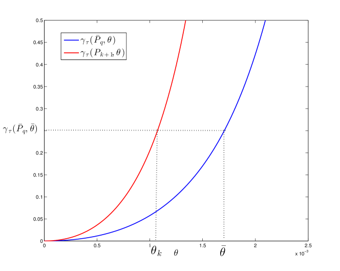
We know that Pk+1P¯qsubscript𝑃𝑘1subscript¯𝑃𝑞P_{k+1}\geq\bar{P}_{q} kqfor-all𝑘𝑞\forall\,k\geq q, which is equivalent to say PkP¯qsubscript𝑃𝑘subscript¯𝑃𝑞P_{k}\geq\bar{P}_{q} kq+1for-all𝑘𝑞1\forall\,k\geq q+1. Then, by Lemma 4.3, condition γτ(Pk+1,θk)=γτ(P¯q,θ¯)subscript𝛾𝜏subscript𝑃𝑘1subscript𝜃𝑘subscript𝛾𝜏subscript¯𝑃𝑞¯𝜃\gamma_{\tau}(P_{k+1},\theta_{k})=\gamma_{\tau}(\bar{P}_{q},\bar{\theta}) implies that

θkθ¯,kq.formulae-sequencesubscript𝜃𝑘¯𝜃for-all𝑘𝑞\displaystyle\theta_{k}\leq\bar{\theta},\;\;\forall\,k\geq q.

Figure 1 shows this situation. Thus, (65) holds if we choose c𝑐c in a such way that θ¯1(1σn(P¯q)ϕN)1τ(1τ)σn(P¯q)¯𝜃1superscript1subscript𝜎𝑛subscript¯𝑃𝑞subscriptitalic-ϕ𝑁1𝜏1𝜏subscript𝜎𝑛subscript¯𝑃𝑞\bar{\theta}\leq\frac{1-(1-\sigma_{n}(\bar{P}_{q})\phi_{N})^{1-\tau}}{(1-\tau)\sigma_{n}(\bar{P}_{q})}.

Refer to caption
Fig. 1: Function γτsubscript𝛾𝜏\gamma_{\tau} with Pk+1P¯qsubscript𝑃𝑘1subscript¯𝑃𝑞P_{k+1}\geq\bar{P}_{q}.
Theorem 4.1.

Let model (3) be such that (A,B)𝐴𝐵(A,B) and (A,C)𝐴𝐶(A,C) are reachable and observable, respectively. Let c𝑐c be such that 0<ccMAX0𝑐subscript𝑐𝑀𝐴𝑋0<c\leq c_{MAX} with

cMAX={γτ(P¯q,1(1σn(P¯q)ϕN)1τ(1τ)σn(P¯q))0τ<1γ1(P¯q,log(1σn(P¯q)ϕN)σn(P¯q))τ=1subscript𝑐𝑀𝐴𝑋casessubscript𝛾𝜏subscript¯𝑃𝑞1superscript1subscript𝜎𝑛subscript¯𝑃𝑞subscriptitalic-ϕ𝑁1𝜏1𝜏subscript𝜎𝑛subscript¯𝑃𝑞0𝜏1subscript𝛾1subscript¯𝑃𝑞1subscript𝜎𝑛subscript¯𝑃𝑞subscriptitalic-ϕ𝑁subscript𝜎𝑛subscript¯𝑃𝑞𝜏1\displaystyle c_{MAX}=\left\{\begin{array}[]{cc}\gamma_{\tau}\left(\bar{P}_{q},\frac{1-(1-\sigma_{n}(\bar{P}_{q})\phi_{N})^{1-\tau}}{(1-\tau)\sigma_{n}(\bar{P}_{q})}\right)&0\leq\tau<1\\ \gamma_{1}\left(\bar{P}_{q},\frac{-\log(1-\sigma_{n}(\bar{P}_{q})\phi_{N})}{\sigma_{n}(\bar{P}_{q})}\right)&\tau=1\end{array}\right. (73)

Nn𝑁𝑛N\geq n and q>0𝑞0q>0 are fixed. Then, for any V0𝒬+nsubscript𝑉0superscriptsubscript𝒬𝑛V_{0}\in\mathcal{Q}_{+}^{n}, the sequence Pksubscript𝑃𝑘P_{k} generated by iteration (18) converges to a unique solution P𝑃P. Moreover, the limit G𝐺G of the filtering gain Gksubscript𝐺𝑘G_{k} as k𝑘k\rightarrow\infty has the property that AGC𝐴𝐺𝐶A-GC is stable.

Proof.

Since

cγτ(P¯q,1(1σn(P¯q)ϕN)1τ(1τ)σn(P¯q)),𝑐subscript𝛾𝜏subscript¯𝑃𝑞1superscript1subscript𝜎𝑛subscript¯𝑃𝑞subscriptitalic-ϕ𝑁1𝜏1𝜏subscript𝜎𝑛subscript¯𝑃𝑞\displaystyle c\leq\gamma_{\tau}\left(\bar{P}_{q},\frac{1-(1-\sigma_{n}(\bar{P}_{q})\phi_{N})^{1-\tau}}{(1-\tau)\sigma_{n}(\bar{P}_{q})}\right),

by Lemma 4.3 we have that (70) holds for kq𝑘𝑞k\geq q and therefore Φ¯N,kϕNInNsubscript¯Φ𝑁𝑘subscriptitalic-ϕ𝑁subscript𝐼𝑛𝑁\bar{\Phi}_{N,k}\leq\phi_{N}I_{nN} for kq~=qN𝑘~𝑞𝑞𝑁k\geq\tilde{q}=\lceil\frac{q}{N}\rceil. Accordingly, the mapping rτ,c,kd()subscriptsuperscript𝑟𝑑𝜏𝑐𝑘r^{d}_{\tau,c,k}(\cdot) is strictly contractive for kq~𝑘~𝑞k\geq\tilde{q}. Since rτ,c,kd()subscriptsuperscript𝑟𝑑𝜏𝑐𝑘r^{d}_{\tau,c,k}(\cdot) is the N𝑁N-fold composition of rc,τ()subscript𝑟𝑐𝜏r_{c,\tau}(\cdot), it follows that the sequence Pksubscript𝑃𝑘P_{k} generated by (18) converges. By (12) the convergence of Pksubscript𝑃𝑘P_{k} implies the convergence of θksubscript𝜃𝑘\theta_{k} to a unique value θ𝜃\theta. Thus, (11) implies the convergence of Vksubscript𝑉𝑘V_{k} to a unique solution V𝑉V. Finally, the stability of AGC𝐴𝐺𝐶A-GC can be proved by applying the Lyapunov stability theory to the algebraic Riccati-like equation

P=(AGC)V(AGC)T+BBT+GGT.𝑃𝐴𝐺𝐶𝑉superscript𝐴𝐺𝐶𝑇𝐵superscript𝐵𝑇𝐺superscript𝐺𝑇\displaystyle P=(A-GC)V(A-GC)^{T}+BB^{T}+GG^{T}.


Finally, it is not difficult to show that the mapping

qγτ(P¯q,1(1σn(P¯q)ϕN)1τ(1τ)σn(P¯q))maps-to𝑞subscript𝛾𝜏subscript¯𝑃𝑞1superscript1subscript𝜎𝑛subscript¯𝑃𝑞subscriptitalic-ϕ𝑁1𝜏1𝜏subscript𝜎𝑛subscript¯𝑃𝑞q\mapsto\gamma_{\tau}\left(\bar{P}_{q},\frac{1-(1-\sigma_{n}(\bar{P}_{q})\phi_{N})^{1-\tau}}{(1-\tau)\sigma_{n}(\bar{P}_{q})}\right)

is nondecreasing. Thus, we have to choose q𝑞q sufficiently large in order to find a bigger cMAXsubscript𝑐𝑀𝐴𝑋c_{MAX}.

5 Example

We consider the constant state space model (3) used in [18],

A𝐴\displaystyle A =[0.1101.2],B=[100010]formulae-sequenceabsentdelimited-[]0.1101.2𝐵delimited-[]100010\displaystyle=\left[\begin{array}[]{cc}0.1&1\\ 0&1.2\\ \end{array}\right],\;\;B=\left[\begin{array}[]{ccc}1&0&0\\ 0&1&0\\ \end{array}\right] (78)
C𝐶\displaystyle C =[11],D=[001].formulae-sequenceabsentdelimited-[]11𝐷delimited-[]001\displaystyle=\left[\begin{array}[]{cc}1&-1\\ \end{array}\right],\;\;D=\left[\begin{array}[]{ccc}0&0&1\\ \end{array}\right]. (81)

The error covariance matrix at time k=0𝑘0k=0 is chosen as V0=I2subscript𝑉0subscript𝐼2V_{0}=I_{2}. We study the convergence of filter (6)-(17) with three different values for τ𝜏\tau: τ=0𝜏0\tau=0, τ=0.5𝜏0.5\tau=0.5 and τ=1𝜏1\tau=1. Fixing q=40𝑞40q=40, N=50𝑁50N=50 we found that

P¯q=102[1.25681.36411.36411.5025],ϕ~N=1.3335103,ϕN=1.3328103.formulae-sequencesubscript¯𝑃𝑞superscript102delimited-[]1.25681.36411.36411.5025formulae-sequencesubscript~italic-ϕ𝑁1.3335superscript103subscriptitalic-ϕ𝑁1.3328superscript103\displaystyle\bar{P}_{q}=10^{2}\cdot\left[\begin{array}[]{cc}1.2568&1.3641\\ 1.3641&1.5025\\ \end{array}\right],\;\;\tilde{\phi}_{N}=1.3335\cdot 10^{-3},\;\;\phi_{N}=1.3328\cdot 10^{-3}. (84)

Moreover, the robust Kalman filter (6)-(17) converges with tolerance in the range [0,cMAX]0subscript𝑐𝑀𝐴𝑋[0,c_{MAX}] where

cMAXsubscript𝑐𝑀𝐴𝑋\displaystyle c_{MAX} =1.22101 for τ=0absent1.22superscript101 for 𝜏0\displaystyle=1.22\cdot 10^{-1}\hbox{ for }\tau=0
cMAXsubscript𝑐𝑀𝐴𝑋\displaystyle c_{MAX} =1.01101 for τ=0.5absent1.01superscript101 for 𝜏0.5\displaystyle=1.01\cdot 10^{-1}\hbox{ for }\tau=0.5
cMAXsubscript𝑐𝑀𝐴𝑋\displaystyle c_{MAX} =8.62102 for τ=1.absent8.62superscript102 for 𝜏1\displaystyle=8.62\cdot 10^{-2}\hbox{ for }\tau=1.

Now, we compare the performances of the following three filters:

  • KF: the standard Kalman filter

  • RKF0: the robust Kalman filter with τ=0𝜏0\tau=0 and c=1.22101𝑐1.22superscript101c=1.22\cdot 10^{-1}

  • RKF05: the robust Kalman filter with τ=0.5𝜏0.5\tau=0.5 and c=1.01101𝑐1.01superscript101c=1.01\cdot 10^{-1}

  • RKF1: the robust Kalman filter with τ=1𝜏1\tau=1 and c=8.62102𝑐8.62superscript102c=8.62\cdot 10^{-2}

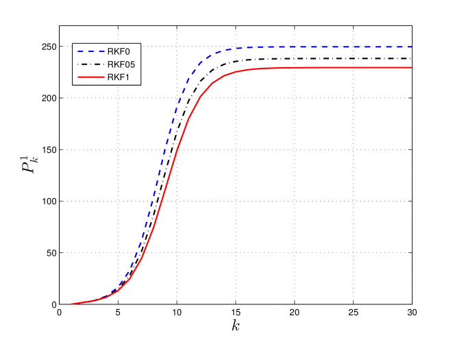
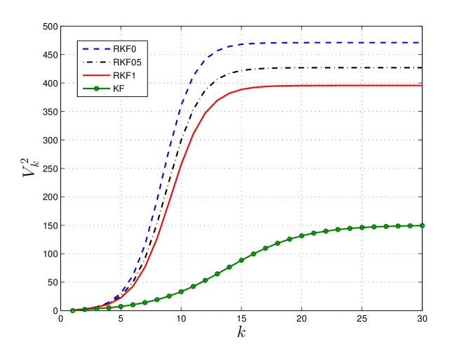
that is we consider the robust Kalman filter with τ=0𝜏0\tau=0, τ=0.5𝜏0.5\tau=0.5, τ=1𝜏1\tau=1 with the corresponding maximum tolerance for which we know that it converges. In Figure 2 we show the pseudo-nominal variance of the state estimation error of the first component of the state, that is the entry of Pksubscript𝑃𝑘P_{k} in position (1,1).

Refer to caption
Fig. 2: Pseudo-nominal variance of the state estimation error of the first component of xksubscript𝑥𝑘x_{k}.

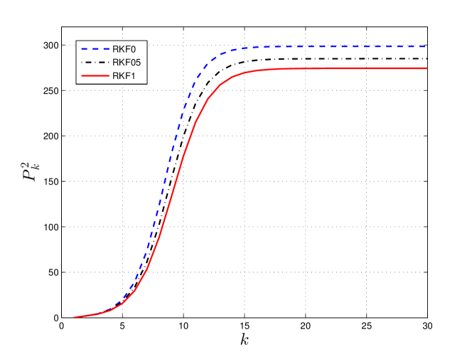
In Figure 3 we show the pseudo-nominal variance of the state estimation error of the second component of xksubscript𝑥𝑘x_{k}, that is the entry in position (2,2) of Pksubscript𝑃𝑘P_{k}.

Refer to caption
Fig. 3: Pseudo-nominal variance of the state estimation error of the second component of xksubscript𝑥𝑘x_{k}.

Roughly speaking these quantities represent the error variance computed using the nominal density fksubscript𝑓𝑘f_{k} but propagating the previous least favorable density f~k1subscript~𝑓𝑘1\tilde{f}_{k-1}. The previous figures show that the Riccati-like iteration converges after 20 steps for τ=0𝜏0\tau=0, τ=0.5𝜏0.5\tau=0.5 and τ=1𝜏1\tau=1. In Figure 4, we show the time-varying risk-sensitivity parameter θksubscript𝜃𝑘\theta_{k} which after 20 steps is already constant.
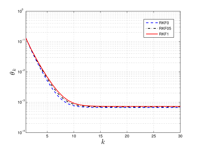
Refer to caption
Fig. 4: Time-varying risk-sensitivity parameter θksubscript𝜃𝑘\theta_{k} in logarithmic scale.

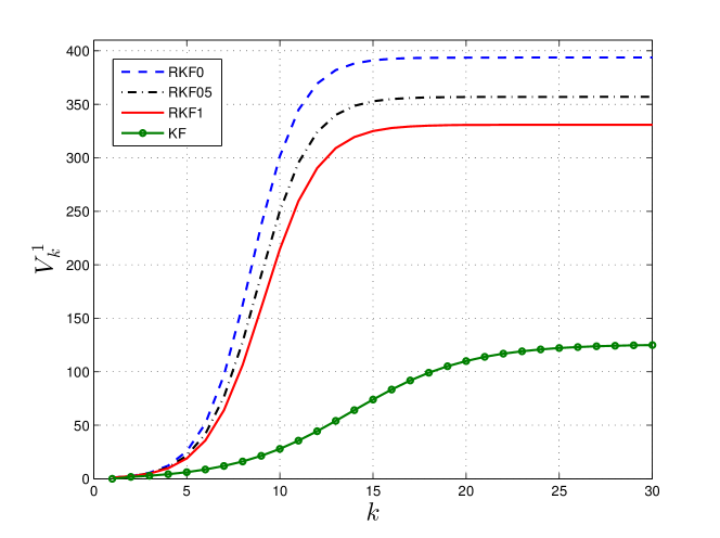
In Figure 5

Refer to caption
Fig. 5: Least-favorable variance of the state estimation error of the first component of xksubscript𝑥𝑘x_{k}.

and Figure 6 we consider the corresponding least-favorable error variance, i.e. the error variance is computed by using the least-favorable density f~ksubscript~𝑓𝑘\tilde{f}_{k} and propagating the previous least favorable density f~k1subscript~𝑓𝑘1\tilde{f}_{k-1}.

Refer to caption
Fig. 6: Least-favorable variance of the state estimation error of the second component of xksubscript𝑥𝑘x_{k}.

It is clear that RKF0, RKF05 and RKF1 are very conservative with respect to the KF, i.e. their error variances are larger than the ones given by KF. This means that, although the upper bound cMAXsubscript𝑐𝑀𝐴𝑋c_{MAX} we found is not tight, the range [0,cMAX]0subscript𝑐𝑀𝐴𝑋[0,c_{MAX}] contains a sufficiently large class of robust estimators. In other words, with c close to zero we have robust Kalman filters with performance similar to KF, while with c𝑐c close to cMAXsubscript𝑐𝑀𝐴𝑋c_{MAX} we have robust Kalman filters very different than KF.

6 Convergence analysis of the τ𝜏\tau-risk sensitive filters

Consider the state-space model (3) and the corresponding nominal joint Gaussian probability density fk(xk+1,yk|Yk1)subscript𝑓𝑘subscript𝑥𝑘1conditionalsubscript𝑦𝑘subscript𝑌𝑘1{f}_{k}(x_{k+1},y_{k}|Y_{k-1}). The family of risk sensitive filters [28] parametrized by τ[0,1]𝜏01\tau\in[0,1] is given by

x^k+1=argmingk𝒢kmaxf~kk,τ𝔼f~k[\displaystyle\hat{x}_{k+1}=\underset{g_{k}\in\mathcal{G}_{k}}{\mathrm{argmin}}\underset{\tilde{f}_{k}\in\mathcal{B}_{k,\tau}}{\max}\mathbb{E}_{\tilde{f}_{k}}[ xk+1gk(yk)2|Yk1]θ1𝒟τ(f~kfk)\displaystyle\|x_{k+1}-g_{k}(y_{k})\|^{2}\,|\,Y_{k-1}]-\theta^{-1}\mathcal{D}_{\tau}(\tilde{f}_{k}\|f_{k}) (85)

where f~ksubscript~𝑓𝑘\tilde{f}_{k} is Gaussian, k,τ={f~k s.t. 𝔻τ(f~kfk)<}subscript𝑘𝜏subscript~𝑓𝑘 s.t. subscript𝔻𝜏conditionalsubscript~𝑓𝑘subscript𝑓𝑘\mathcal{B}_{k,\tau}=\{\tilde{f}_{k}\hbox{ s.t. }\mathbb{D}_{\tau}(\tilde{f}_{k}\|f_{k})<\infty\} and 𝒢ksubscript𝒢𝑘\mathcal{G}_{k} is the set of estimators for which the objective function in (85) is finite. θ>0𝜃0\theta>0 is the risk sensitivity parameter. The second term in the objective function in (85) is always nonpositive because 𝔻τ(f~kfk)0subscript𝔻𝜏conditionalsubscript~𝑓𝑘subscript𝑓𝑘0\mathbb{D}_{\tau}(\tilde{f}_{k}\|f_{k})\geq 0. Therefore, for large values of θ𝜃\theta the maximizer has the possibility to take a probability density far from the nominal one. The τ𝜏\tau-risk sensitive filter (85) thus represents a relaxed version of the robust Kalman filter (6)-(17) where θ𝜃\theta now is constant and fixed by the user. For the case τ=0𝜏0\tau=0 we obtain the usual risk sensitive filter [3]. The resulting estimator obeys the recursion (6)-(8) with

Vk+1={LPk+1(Inθ(1τ)LPk+1TLPk+1)1τ1LPk+1T,0<τ<1LPk+1exp(θLPk+1TLPk+1)LPk+1T,τ=1.subscript𝑉𝑘1casessubscript𝐿subscript𝑃𝑘1superscriptsubscript𝐼𝑛𝜃1𝜏superscriptsubscript𝐿subscript𝑃𝑘1𝑇subscript𝐿subscript𝑃𝑘11𝜏1superscriptsubscript𝐿subscript𝑃𝑘1𝑇0𝜏1subscript𝐿subscript𝑃𝑘1𝜃superscriptsubscript𝐿subscript𝑃𝑘1𝑇subscript𝐿subscript𝑃𝑘1superscriptsubscript𝐿subscript𝑃𝑘1𝑇𝜏1\displaystyle V_{k+1}=\left\{\begin{array}[]{ll}L_{P_{k+1}}\left(I_{n}-\theta(1-\tau)L_{P_{k+1}}^{T}L_{P_{k+1}}\right)^{\frac{1}{\tau-1}}L_{P_{k+1}}^{T},&0<\tau<1\\ L_{P_{k+1}}\exp\left(\theta L_{P_{k+1}}^{T}L_{P_{k+1}}\right)L_{P_{k+1}}^{T},&\tau=1.\end{array}\right. (88)

The study of the asymptotic behavior of the τ𝜏\tau-risk sensitive filter requires to consider two different cases: the case 0<τ<10𝜏10<\tau<1 and the case τ=1𝜏1\tau=1.

In the former case, the Riccati-like iteration has the same form of (18) but the image of 𝒬+nsuperscriptsubscript𝒬𝑛\mathcal{Q}_{+}^{n} under this mapping is not entirely contained in 𝒬+nsuperscriptsubscript𝒬𝑛\mathcal{Q}_{+}^{n}. The reason is that condition Vk>0subscript𝑉𝑘0V_{k}>0 holds only if Pksubscript𝑃𝑘P_{k} is such that 0<Pk<(θ(1τ))1In0subscript𝑃𝑘superscript𝜃1𝜏1subscript𝐼𝑛0<P_{k}<(\theta(1-\tau))^{-1}I_{n} and this condition could be not satisfied. Following similar arguments used in [18] for the case τ=0𝜏0\tau=0, it is possible to find conditions on V0subscript𝑉0V_{0} and θ𝜃\theta for which the trajectory of iteration (18) satisfies Vk>0subscript𝑉𝑘0V_{k}>0 for any k>0𝑘0k>0. However, these conditions on V0subscript𝑉0V_{0} and θ𝜃\theta are rather intricate and require to design a gain matrix and a scaling factor ρ2superscript𝜌2\rho^{2}.

For the case τ=1𝜏1\tau=1, Vksubscript𝑉𝑘V_{k} is positive definite, and thus well defined, whenever Pksubscript𝑃𝑘P_{k} is positive definite. Accordingly, the image of 𝒬+nsuperscriptsubscript𝒬𝑛\mathcal{Q}_{+}^{n} under the corresponding mapping, denoted by rτ=1,θ()subscript𝑟𝜏1𝜃r_{\tau=1,\theta}(\cdot), is 𝒬+nsuperscriptsubscript𝒬𝑛\mathcal{Q}_{+}^{n}. Thus, the convergence of the iteration is guaranteed by only imposing conditions on the risk sensitivity parameter θ𝜃\theta.

Theorem 6.1.

Let model (3) be such that (A,B)𝐴𝐵(A,B) and (A,C)𝐴𝐶(A,C) are reachable and observable, respectively. Let θ𝜃\theta be such that

θlog(1σn(P¯q)ϕN)σn(P¯q),𝜃1subscript𝜎𝑛subscript¯𝑃𝑞subscriptitalic-ϕ𝑁subscript𝜎𝑛subscript¯𝑃𝑞\displaystyle\theta\leq\frac{-\log(1-\sigma_{n}(\bar{P}_{q})\phi_{N})}{\sigma_{n}(\bar{P}_{q})}, (89)

Nn𝑁𝑛N\geq n and q>0𝑞0q>0 are fixed. Then, for any V0𝒬+nsubscript𝑉0superscriptsubscript𝒬𝑛V_{0}\in\mathcal{Q}_{+}^{n}, the sequence Pksubscript𝑃𝑘P_{k} generated by the risk-sensitive filter with τ=1𝜏1\tau=1 converges to a unique solution P𝑃P. Moreover, the limit G𝐺G of the filtering gain Gksubscript𝐺𝑘G_{k} as k𝑘k\rightarrow\infty has the property that AGC𝐴𝐺𝐶A-GC is stable.

Proof.

We consider the downsampled process xkdsuperscriptsubscript𝑥𝑘𝑑x_{k}^{d} with xkd=xkNsuperscriptsubscript𝑥𝑘𝑑subscript𝑥𝑘𝑁x_{k}^{d}=x_{kN} and the corresponding time-varying Riccati-iteration is Pk+1d=rτ,θ,kd(Pkd)superscriptsubscript𝑃𝑘1𝑑subscriptsuperscript𝑟𝑑𝜏𝜃𝑘superscriptsubscript𝑃𝑘𝑑P_{k+1}^{d}=r^{d}_{\tau,\theta,k}(P_{k}^{d}) where rτ,θ,kd()subscriptsuperscript𝑟𝑑𝜏𝜃𝑘r^{d}_{\tau,\theta,k}(\cdot) has the same structure of (60). Let Φk=Pk+11Vk+11subscriptΦ𝑘superscriptsubscript𝑃𝑘11superscriptsubscript𝑉𝑘11\Phi_{k}=P_{k+1}^{-1}-V_{k+1}^{-1}. Proposition 3.1 still holds. In particular, there exists ϕNsubscriptitalic-ϕ𝑁\phi_{N} such that if (65) holds then the matrices ΩΦ¯N,ksubscriptΩsubscript¯Φ𝑁𝑘\Omega_{\bar{\Phi}_{N,k}} and WΦ¯N,ksubscript𝑊subscript¯Φ𝑁𝑘W_{\bar{\Phi}_{N,k}} are positive definite. Accordingly, by Lemma 2.1 the N𝑁N-fold mapping rτ,θ,kd()subscriptsuperscript𝑟𝑑𝜏𝜃𝑘r^{d}_{\tau,\theta,k}(\cdot) is strictly contractive and thus also rτ=1,θ()subscript𝑟𝜏1𝜃r_{\tau=1,\theta}(\cdot) is strictly contractive. Lemma 4.1 and Lemma 4.2 still hold, in particular

Φk1eσn(P¯q)θσn(P¯q)In,kq+1.formulae-sequencesubscriptΦ𝑘1superscript𝑒subscript𝜎𝑛subscript¯𝑃𝑞𝜃subscript𝜎𝑛subscript¯𝑃𝑞subscript𝐼𝑛for-all𝑘𝑞1\displaystyle\Phi_{k}\leq\frac{1-e^{-\sigma_{n}(\bar{P}_{q})\theta}}{\sigma_{n}(\bar{P}_{q})}I_{n},\;\;\forall\;k\geq q+1.

Finally, by imposing

1eσn(P¯q)θσn(P¯q)ϕN,1superscript𝑒subscript𝜎𝑛subscript¯𝑃𝑞𝜃subscript𝜎𝑛subscript¯𝑃𝑞subscriptitalic-ϕ𝑁\displaystyle\frac{1-e^{-\sigma_{n}(\bar{P}_{q})\theta}}{\sigma_{n}(\bar{P}_{q})}\leq\phi_{N},

which coincides with (89), then condition (65) holds. Thus, the sequence Pksubscript𝑃𝑘P_{k} converges to a unique P𝑃P as k𝑘k\rightarrow\infty. The stability of AGC𝐴𝐺𝐶A-GC follows as before.  

It is clear that condition (89) on the risk sensitivity parameter is easy to check. Accordingly, this filter is preferable than the risk-sensitive filter with 0τ<10𝜏10\leq\tau<1.

7 Conclusions

A convergence analysis of a family of robust Kalman filters has been presented. This analysis exploited the fact that the N𝑁N-fold Riccati mapping, which is given by downsampling these filters, is strictly contractive provided that the time-varying risk-sensitive parameter is sufficiently small. This condition is then guaranteed by placing an upper bound on the tolerance parameter of the robust filters. Finally, we have studied the convergence property of a family of risk-sensitive filters which can be understood as a relaxed version of the previous robust Kalman filters.

References

  • [1] J. Aubin and I. Ekeland, Applied Nonlinear Analysis, J. Wiley, New York, 1984.
  • [2] R. Bhatia, On the exponential metric increasing property, Linear Algebra and its Appl., 375 (2003), pp. 211–220.
  • [3] R. Boel, M. James, and I. Petersen, Robustness and risk-sensitive filtering, IEEE Trans. Automat. Control, 47 (2002), pp. 451–461.
  • [4] P. Bougerol, Kalman filtering with random coefficients and contractions, SIAM J. Control and Optimiz., 31 (1993), pp. 942–959.
  • [5] A. Ferrante and B. Levy, Hermitian solutions of the equation x=q+nx1n𝑥𝑞𝑛superscript𝑥1superscript𝑛x=q+nx^{-1}n^{*} , Linear Algebra and its Applications, 247 (1996), pp. 359–373.
  • [6] A. Ferrante and L. Ntogramatzidis, The generalised discrete algebraic riccati equation in linear-quadratic optimal control, Automatica, 49 (2013), pp. 471–478.
  • [7] A. Ferrante and L. Ntogramatzidis, The generalized continuous algebraic riccati equation and impulse-free continuous-time LQ optimal control, Automatica, 50 (2014), pp. 1176–1180.
  • [8] S. Gaubert and Z. Qu, The contraction rate in thompson’s part metric of order-preserving flows on a cone - application to generalized riccati equations, Journal of Differential Equations, 256 (2014), pp. 2902–2948.
  • [9] L. Hansen and T. Sargent, Robustness, Princeton University Press, Princeton, NJ, 2008.
  • [10] B. Hassibi, A. Sayed, and T. Kailath, Linear estimation in Krein spaces. I. Theory, IEEE Trans. Automat. Control, 41 (1996), pp. 18–33.
  • [11]  , Linear estimation in Krein spaces. II. Applications, IEEE Trans. Automat. Control, 41 (1996), pp. 34–49.
  • [12]  , Indefinite-Quadratic Estimation and Control- A Unified Approach to H2superscript𝐻2H^{2} and Hsuperscript𝐻H^{\infty} Theories, Soc. Indust. Appl. Math., Philadelphia, 1999.
  • [13] J. Lawson and Y.Lim, The symplectic semigroup and Riccati differential equations, J. Dynamical and Control Syst., 12 (2006), pp. 49–77.
  • [14]  , A Birkhoff contraction formula with applications to Riccati equations, SIAM J. Control and Optimiz., 46 (2007), pp. 930–951.
  • [15] H. Lee and Y. Lim, Invariant metrics, contractions and nonlinear matrix equations, Nonlinearity, 2 (2008), pp. 857–878.
  • [16] B. Levy and R. Nikoukhah, Robust least-squares estimation with a relative entropy constraint, Information Theory, IEEE Transactions on, 50 (2004), pp. 89–104.
  • [17] B. Levy and R. Nikoukhah, Robust state-space filtering under incremental model perturbations subject to a relative entropy tolerance, IEEE Trans. Automat. Control, 58 (2013), pp. 682–695.
  • [18] B. C. Levy and M. Zorzi, A contraction analysis of the convergence of risk-sensitive filters, SIAM Journal on Control and Optimization, 54 (2016), pp. 2154–2173.
  • [19] J. Speyer, C. Fan, and R. Banavar, Optimal stochastic estimation with exponential cost criteria, in Proc. 31st IEEE Conf. Decision Control, Tucson, AZ, Dec. 1992, pp. 2293–2298.
  • [20] A. Thompson, On certain contraction mappings in a partially ordered vector space, Proceedings of the American Mathematical Society, 14 (1963), pp. 438–443.
  • [21] P. Whittle, Risk-sensitive Optimal Control, J. Wiley, Chichester, England, 1980.
  • [22] A. Zenere and M. Zorzi, Model predictive control meets robust Kalman filtering, IFAC Proceedings Volumes (to appear), (2017).
  • [23] M. Zorzi, A new family of high-resolution multivariate spectral estimators, IEEE Transactions on Automatic Control, 59 (2014), pp. 892–904.
  • [24] M. Zorzi, Rational approximations of spectral densities based on the alpha divergence, Mathematics of Control, Signals, and Systems, 26 (2014), pp. 259–278.
  • [25] M. Zorzi, An interpretation of the dual problem of the THREE-like approaches, Automatica, 62 (2015), pp. 87–92.
  • [26]  , Multivariate spectral estimation based on the concept of optimal prediction, IEEE Transactions on Automatic Control, 60 (2015), pp. 1647–1652.
  • [27] M. Zorzi, On the robustness of the Bayes and Wiener estimators under model uncertainty, Submitted, arXiv:1508.01904, (2015).
  • [28] M. Zorzi, Robust Kalman filtering under model perturbations, IEEE Transactions on Automatic Control, 62 (2017).
  • [29] M. Zorzi and B. C. Levy, On the convergence of a risk sensitive like filter, in 54th IEEE Conference on Decision and Control (CDC), Dec 2015, pp. 4990–4995.