Joint Transmission with Limited Backhaul Connectivity

Abstract

Downlink beamforming techniques with low signaling overhead are proposed for joint processing coordinated (JP) multi-point transmission. The objective is to maximize the weighted sum rate within joint transmission clusters. As the considered weighted sum rate maximization is a non-convex problem, successive convex approximation techniques, based on weighted mean-squared error minimization, are applied to devise algorithms with tractable computational complexity. Decentralized algorithms are proposed to enable JP even with limited backhaul connectivity. These algorithms rely provide a variety of alternatives for signaling overhead, computational complexity and convergence behavior. Time division duplexing is exploited to design transceiver training techniques for two scenarios: stream specific estimation and direct estimation. In the stream specific estimation, the base station and user equipment estimate all of the stream specific precoded pilots individually and construct the transmit/receive covariance matrices based on these pilot estimates. With the direct estimation, only the intended transmission is separately estimated and the covariance matrices constructed directly from the aggregate system-wide pilots. The proposed training schemes incorporate bi-directional beamformer signaling to improve the convergence behavior. This scheme exploits the time division duplexing frame structure and is shown to improve the training latency of the iterative transceiver design. The impact of feedback/backhaul signaling quantization is considered, in order to further reduce the signaling overhead. Also, user admission is being considered for time-correlated channels. The enhanced transceiver convergence rate enables periodic beamformer reinitialization, which greatly improves the achieved system performance in dense networks.

I Introduction

Cooperative transmission schemes and spatial domain interference managements are the foundation of the modern cellular and heterogeneous wireless systems. The ever increasing need for spectral efficiency, imposes demand for effective interference management and transmission coordination. The current wireless standards already support efficient single cell MIMO beamforming, which allows smart beamformer design to efficiently take advantage of the multi-user diversity in the spatial domain [1]. Also, the basic operation of virtual MIMO has been preliminarily covered by the LTE-A standards. This also includes support for fully centralized JP CoMP transmission schemes, which from the theoretical perspective does not differ much from single cell MIMO beamformer processing. Still, the practical limitations in BS backhaul connectivity are preventing effective implementation of more advanced JP CoMP schemes. Multi-cell beam coordination is still in somewhat elementary stages when considering the current LTE-A standardization [1]. On the other hand, a lot of research effort has been invested in CB for multi-cell systems. Much of this research has been focusing on decentralized coordination strategies with low backhaul signaling overhead in mind [2, 3, 4, 5, 6]. These techniques are still limited in the DoF sense and fall short in exploiting the available opportunities of the increasingly dense cell networks. Most of the CB research effort is focused on mitigating and managing the inter-cell interference, as it is the foremost barrier preventing efficient spectrum utilization especially, in dense heterogeneous networks. To this end, JP CoMP transmission techniques have been considered, where the neighboring BS cooperate on different levels, in order to increase the available DoF and alleviate the detrimental interference conditions in multi-cell systems [7, 8, 9].

JP CoMP, in general, requires high bandwidth and low latency BS inter-connectivity, which is hard to realize in conventional multi-cell systems. This has led to development of network architectures that make virtual MIMO operation realizable and offer the required centralized coordination. The most popular architectures in today’s JP research are the CRAN [10]. In CRAN the BS are connected to a CU over high capacity and low latency backhaul links. This allows the CU to perform centralized processing and the BS act merely as RRH. The CU can use JP to utilize simultaneously multiple RRH for beamforming. Although the backhaul limitations of CoMP transmission systems have been addressed in various publications, most of the JP CoMP research allows full CSI exchange and centralized processing which greatly simplifies the beamformer design [11, 8, 4, 12, 13]. While the global CSI exchanged is common assumption for JP designs, in many cases, it may not be feasible in practice. The latency and mobility requirements often prevent accurate CSI exchange even in modest scale [9].

This paper focuses on JP CoMP with WSRMax and limited backhaul capacity, i.e., without full CSI exchange. The backhaul limitations prevent the BS from sharing the global CSI within the cooperating clustering. Thus, the limited signaling possibilities require the BS to perform partially independent beamformer design even within the cooperating JP clustering. This has motivated us to design decentralized transceiver processing with limited signaling overhead. Still, we assume that the transmitted data can be shared among the serving BS. The data can be queued and prioritized by a central processing node, which then distributes it to the serving BS. This makes the data less sensitive to the latency in the system.

Along with low signaling overhead, we also consider different transceiver training techniques depending on the pilot planning and contamination when using TDD. Basically, we divide the problem into two scenarios: SSE and DE. In SSE, we assume that all pilot sequences are orthogonal and orthogonal. With DE, we allow non-orthogonal noisy pilots, which is sensible in more crowded environments.

I-A Prior Work

CB has extensively studied with respect to decentralized inter-cell interference coordination. In CB, the interfering BS cooperatively coordinate the beamformers and schedule their UE, is such a way that the inter-cell interference conditions are not detrimental for the neighboring cells. CB can be efficiently performed with limited signaling overhead as shown, e.g., in [4, 2, 3]. WSRMax with CB have been studied, e.g., in [14, 15, 16]. Over the last ten years, many practical CB schemes have been proposed with reasonable signaling overhead and computational complexity. The most popular approach is via the, so called, WMMSE design, where the problem is equivalently presented as logarithmic MSE minimization problem. This problem is still non-convex and SCA is applied on the non-convex objective. This results in iteratively weighted MSE minimization, which can be efficiently solved. The WMMSE method was first proposed in [16]. In [2], WMMSE was shown to have naturally decentralized processing structure for cellular TDD MIMO systems. Efficient signaling techniques for WMMSE were proposed in [3]. Similar approach to WSRMax has also been considered in [5, 17, 18]. The methods proposed in [16, 2] are readily applicable to jointly coherent centralized CoMP beam coordination, as the problem closely resembles a conventional single-cell coordinated WSRMax problem. Since JP inherently couples the beamformer processing between the cooperating BS, the decentralized CB methods cannot be used as is. Developing the decentralized CoMP designs is one of the focus points of this paper.

In JP, the backhaul information can be handled in one of two ways: 1. In data sharing, the CU exchanges the user specific messages with the ̵̧cooperating BS explicitly and the joint beamformers are informed separately [19]. 2. Using compression, the messages can be precoded beforehand at the CU and only the compressed version of the analog beamformer is informed to the BS [20, 21]. As of now, the data sharing strategy has been more popular approach, mostly due to the lower complexity and easier modeling of the explicit backhaul constraints. Sparsity imposing joint beamformer designs are the most common approach for backhaul limited CoMP design. The sparse joint beamforming has been considered, e.g., in [19, 22, 23, 24]. These designs try to limit the sizes of the JP clusters and, thus, implicitly reduce the backhaul overhead. The compression approach has recently gained more popularity [20, 25, 26, 21] Different aspects and benefits of backhaul compression have been studied, for example, in [20, 25, 26, 21]. The data sharing and compression strategies for energy efficient communication and backhaul power consumption were compared in [21].

Decentralized interference management has been a major research interest in the cellular beamformer design. The backhaul delay and capacity limitations have motivated CB research to find solutions beyond the centralized processing concepts. Most of this research has focused on decomposition techniques of convex beamformer optimization problems [4, 27]. For CB, the WSRMax has been shown to have decoupled structure when SCA is applied [16, 2]. More generalized frameworks have also been proposed. For example, a general BR framework, which allows straightforward parallel processing for varying performance objectives, was proposed in [17].

Pilot non-orthogonality and contamination has been widely studied, albeit, not in the context of JP CoMP. More generally, the impact of imperfect CSI has been a popular topic in the literature. The impact of partial or imperfect CSI feedback to CB and JP has been studied in various publications, e.g., [8, 28, 29]. Partially available CSI imposes a different problem to the one considered herein. With imperfect CSI, the problem is more sensitive to the management of the CSI uncertainty. The pilot contamination in TDD based transceiver training for coordinated beamforming has been considered, e.g., in [30, 31, 32]. In [31, 32], direct LS beamformer estimation from the contaminated UL/DL pilots was shown to provide good performance as opposed to trying to estimate the individual channels.

I-B Contributions

We provide WSRMax design JP CoMP with emphasis on systems with moderately fast fading channel conditions We assume data sharing, where the CU provides the data for cooperating BS. The transceiver processing is done with minimal CU involvement by novel decentralized CoMP beamformer designs. Our focus is on practically realizable signaling schemes and efficient user admission. We extend the decentralized sum-MSE minimizing JP scheme proposed in [33] to perform WMMSE with multi-antenna transmitters and receivers. We employ BR, ADMM and SG schemes to provide decentralized algorithms with different performance properties and signaling overhead. We also consider pilot contamination with DE methods and provide efficient decentralized processing via SG for the case with imperfect channel estimation as well. We utilize a bi-directional signaling scheme with similar frame structure as in [31]. This allows fast signaling iterations by incorporating the training sequence into the transmitted frame structure. Furthermore, we propose a novel periodic beamformer reinitialization scheme, which is shown to significantly improve the user admission performance in time correlated fading environment. The performance of the proposed method is evaluated in a cellular multi-user network with a time correlated channel model.

Contributions of this paper are summarized as follows:

• BR, ADMM and SG based decentralized beamforming are proposed for stream specific SSE.

• Beamformer DE with SG based decentralized beamforming procedures are considered.

• User admission, bi-directional training and feedback quantization techniques are considered for time-correlated CoMP processing.

• Performance of the proposed methods are studied with numerical examples in time correlated channels.

I-C Organization and Notation

The rest of the paper is organized as follows. The system model is given in Section II. In Section III, the considered WSRMax problem is described along with the WMMSE SCA design. The beamformer designs with SSE are given in Section IV. DE is considered in Section V. Bi-directional training and feedback quantization are discussed in Section VI. Finally, the numerical examples and concluding remarks are given in Sections VIII and IX, respectively.

Notation: Matrices and vectors are presented by boldface upper and lower case letters, respectively. Transpose of matrix $\mathbf{A}$ is denoted as $\mathbf{A}^{\mbox{\scriptsize T}}$ and, similarly, conjugate transpose is denoted as $\mathbf{A}^{\mbox{\scriptsize H}}$. Conventional matrix inversion is written as $\mathbf{A}^{-1}$, whereas $\mathbf{A}^{\dagger}$ presents the pseudoinverse of matrix $\mathbf{A}$. Mapping of negative scalars to zero is written as ${(\cdot)}^{+}=\max(0,\cdot)$. Cardinality of a discrete set $\mathcal{A}$ is given by $|\mathcal{A}|$. Expected value of a random variable is denoted by $\mathbb{E}[\cdot]$.

II System Model

We consider a multi-cell system with $B$ BS each equipped with $N_{\text{T}}$ transmit antennas. There are, in total, $K$ UE each equipped with $N_{\text{R}}$ receive antennas. Each UE $k=1,\ldots,K$ is coherently served by $|\mathcal{B}_{k}|$ BS, where set $\mathcal{B}_{k}$ defines the joint processing cluster (coherent serving BS indices) for UE $k$. Similarly, the set of UE indices served by BS $b=1,\ldots,B$ is denoted by $\mathcal{C}_{b} =\{k|b\in\mathcal{B}_{k},k=1,\ldots,K\}$. The set of all UE indices is given by $\mathcal{K}=\{1,\ldots,K\}$. The maximum number of spatial data streams allocated to UE $k=1,\ldots,K$ is denoted by $L_{k}\leq\min\left(|\mathcal{B}_{k}|N_{\text{T}},N_{\text{R}}\right)$. To simplify the notation in various places, we use the following set abbreviations: $(k,l)\triangleq\{(k,l)|k\in\mathcal{K},l=1,\ldots,L_{k}\}$ and $(b,k,l)\triangleq\{(b,k,l)|k\in\mathcal{K},l=1,\ldots,L_{k},b\in\mathcal{B}_{k}\}$. The considered system model is illustrated in Fig. 1.

Figure 1: Simplified system model with $B=4$ cooperating BS and $K=6$ UE that are split into two JP clusters.

The downlink transmission within the JP set is considered to be symbol synchronous in the sense that each transmitted symbol from $\mathcal{B}_{k},k=1,\ldots,K$ is coherently combined at all UE. Only the local CSI knowledge is assumed, that is, each BS $b=1,\ldots,B$ is only aware of the channel matrix $\mathbf{H}_{b,k}\in\mathbb{C}^{N_{\text{R}}\times N_{\text{T}}}\ \forall\ k=1,\ldots,K$, while the data sharing is assumed within each serving set of BS $\mathcal{B}_{k}$. Furthermore, we assume TDD, which imposes strong correlation between the UL and DL channels.

The received signal at UE $k=1,\ldots,K$ is given as

$$\mathbf{y}_{k}=\sum_{i=1}^{K}\sum_{b\in\mathcal{B}_{i}}\sum_{j=1}^{L_{i}}\mathbf{H}_{b,k}\mathbf{m}_{b,i,j}d_{i,j}+\mathbf{n}_{k}\text{,}$$ (1)

where $\mathbf{m}_{b,i,j}\in\mathbb{C}^{N_{\text{T}}}$ is the beamformer vector for the $j^{th}$ spatial data stream of UE $i$ from BS $b$ and $\mathbf{n}_{k}\sim\mathcal{CN}(0,\sigma_{k}^{2}\mathbf{I})$ denotes the receiver noise. The complex data symbols $d_{k,l},k=1,\ldots,K,l=1,\ldots,L_{k}$ are assumed to be i.i.d. with $\mathbb{E}\{|d_{k,l}|^{2}\}=1$.

The estimated symbol at UE $k=1,\ldots,K$ over stream $l$, after the applying receive beamformer $\mathbf{u}_{k,l}\in\mathbb{C}^{N_{\text{R}}}$, is given as $\hat{d}_{k,l}=\mathbf{u}_{k,l}^{\mbox{\scriptsize H}}\mathbf{y}_{k}$. The resulting SINR is

$$\begin{array}[]{rl}\displaystyle\Gamma_{k,l}=\frac{\displaystyle|\sum_{b\in\mathcal{B}_{k}}\mathbf{u}_{k,l}^{\mbox{\scriptsize H}}\mathbf{H}_{b,k}\mathbf{m}_{b,k,l}|^{2}}{\displaystyle\sum_{i=1}^{K}\sum_{\begin{subarray}{c}j=1,\\ (i,j)\neq(k,l)\end{subarray}}^{L_{i}}|\sum_{b\in\mathcal{B}_{i}}\mathbf{u}_{k,l}^{\mbox{\scriptsize H}}\mathbf{H}_{b,k}\mathbf{m}_{b,i,j}|^{2}+\|\mathbf{u}_{k,l}\|^{2}\sigma^{2}_{k}}\end{array}\text{,}$$ (2)

and the corresponding MSE is

$$\begin{array}[]{rl}\displaystyle\epsilon_{k,l}\triangleq&\displaystyle\mathbb{E}[|d_{k,l}-\hat{d}_{k,l}|^{2}]\\ =&\displaystyle|\sum_{b\in\mathcal{B}_{k}}\mathbf{u}_{k,l}^{\mbox{\scriptsize H}}\mathbf{H}_{b,k}\mathbf{m}_{b,k,l}-1|^{2}+\|\mathbf{u}_{k,l}\|^{2}\sigma_{k}^{2}+\\ &\displaystyle\sum_{i=1}^{K}\sum_{\begin{subarray}{c}j=1,\\ (i,j)\neq(k,l)\end{subarray}}^{L_{i}}|\sum_{b\in\mathcal{B}_{i}}\mathbf{u}_{k,l}^{\mbox{\scriptsize H}}\mathbf{H}_{b,k}\mathbf{m}_{b,i,j}|^{2}\text{.}\end{array}$$ (3)

Note that (3) is a convex function in terms of the transmit beamformers $\mathbf{m}_{b,k,l}\ \forall\ (b,k,l)$ for fixed receivers $\mathbf{u}_{k,l}\ \forall\ (k,l)$.

III Problem Formulation & Centralized Solution

We consider WSRMax subject to BS specific sum transmit power constraints. The general problem can be given as

$$\begin{array}[]{rl}\underset{\begin{subarray}{c}\mathbf{u}_{k,l},\mathbf{m}_{b,k,l}\end{subarray}}{\max.}&\displaystyle\sum_{k=1}^{K}\sum_{l=1}^{L_{k}}\mu_{k}\log_{2}\left(1+\Gamma_{k,l}\right)\\ \mathrm{s.\ t.}&\displaystyle\sum_{k\in\mathcal{C}_{b}}^{K}\sum_{l=1}^{L_{k}}\|\mathbf{m}_{b,k,l}\|^{2}\leq P_{b},\ b=1,\ldots,B\text{,}\end{array}$$ (4)

where $\mu_{k},k=1,\ldots,K$ are the user priority weights. The problem is non-convex and known to be NP-hard [34]. The optimal, i.e., rate maximizing, receive beamformers for (4) are the MMSE receive beamformers

$$\mathbf{u}_{k,l}=\mathbf{K}_{k}^{-1}\left(\sum_{b\in\mathcal{B}_{k}}\mathbf{H}_{b,k}\mathbf{m}_{b,k,l}\right)\text{,}$$ (5)

where $\mathbf{K}_{k}=\sum_{i=1}^{K}\sum_{j=1}^{L_{i}}\sum_{b\in\mathcal{B}_{i}}\mathbf{H}_{b,k}\mathbf{m}_{b,i,j}\mathbf{m}_{b,i,j}^{\mbox{\scriptsize H}}\mathbf{H}_{b,k}^{\mbox{\scriptsize H}}+\mathbf{I}\sigma_{k}^{2}\text{.}$

It is well-known that, when the MMSE receive beamformers are applied, there is an inverse relation between the SINR and the corresponding MSE [2]

$$\epsilon_{k,l}^{-1}=1+\Gamma_{k,l}\text{.}$$ (6)

Now, applying (6) to (4) we can formulate the weighted sum rate maximization problem as

$$\begin{array}[]{rl}\underset{\begin{subarray}{c}\mathbf{u}_{k,l},\mathbf{m}_{b,k,l}\end{subarray}}{\min.}&\displaystyle\sum_{k=1}^{K}\sum_{l=1}^{L_{k}}\mu_{k}\log_{2}\left(\epsilon_{k,l}\right)\\ \mathrm{s.\ t.}&\displaystyle\sum_{k\in\mathcal{C}_{b}}^{K}\sum_{l=1}^{L_{k}}\|\mathbf{m}_{b,k,l}\|^{2}\leq P_{b},\ b=1,\ldots,B\text{.}\end{array}$$ (7)

Since (7) is not jointly convex for the transmit and receive beamformers, we consider an alternating design, where the transmit and receive beamformers are solved in separate instances. This separation is convenient for TDD processing as the DL and UL transmissions are temporally separated. With fixed transmit beamformers $\mathbf{m}_{b,k,l}\ \forall\ (b,k,l)$, the optimal receive beamformer can be obtained from (5) [16]. This can be easily verified from the first-order KKT conditions. As (7) is still non-convex, even for fixed receive beamformers, we need to apply an iterative convex approximation algorithm to generate the transmit beamformers. We employ WMMSE [16, 2] to formulate transmit beamformer design algorithm with tractable complexity and convex steps.

The main idea in the WMMSE is to perform successive first-order approximation of the non-convex objective in (7). The objective is separable in terms of $\epsilon_{k,l}\ \forall\ (k,l)$. Thus, we can approximate each term individually. In iteration $n$, the first-order approximation in terms of $\epsilon_{k,l}$, at point $\epsilon_{k,l}^{(n)}$, can be given as

$$\log_{2}\left(\epsilon_{k,l}\right)\approx\frac{1}{\log(2)\epsilon_{k,l}^{(n)}}\left(\epsilon_{k,l}-\epsilon_{k,l}^{(n)}\right)+\log_{2}\left(\epsilon_{k,l}^{(n)}\right)\text{.}$$ (8)

When optimizing over the approximated objective, the constant terms have no impact on the solution and can, thus, be neglected. Now, the approximated transmit beamformer design subproblem can be given as a WMMSE problem

$$\begin{array}[]{rl}\underset{\begin{subarray}{c}\mathbf{m}_{b,k,l}\end{subarray}}{\min.}&\displaystyle\sum_{k=1}^{K}\sum_{l=1}^{L_{k}}w^{(n)}_{k,l}\epsilon_{k,l}\\ \mathrm{s.\ t.}&\displaystyle\sum_{k\in\mathcal{C}_{b}}^{K}\sum_{l=1}^{L_{k}}\|\mathbf{m}_{b,k,l}\|^{2}\leq P_{b},\ b=1,\ldots,B\text{,}\end{array}$$ (9)

where

$$w^{(n)}_{k,l}=\frac{\mu_{k}}{\log(2)\epsilon_{k,l}^{(n)}}\ \forall\ (k,l)\text{.}$$ (10)

Since the MSE terms (3) are convex for fixed receive beamformers, (9) is a convex problem and, as such, efficiently solvable. The complete centralized algorithm is outlined in Algorithm 1. As shown in [2], the successive approximation algorithm provides monotonic convergence of the objective function and convergence to a local stationary point of the original problem (4). Alternatively, we could have also applied extended WSRMax techniques such as the ones proposed in [18], where the authors propose an SCA approach with improved rate of convergence.

Algorithm 1 Centralized WMMSE algorithm.

1:  Initialize feasible $\mathbf{m}_{b,k,l}\ \forall\ (b,k,l)$ and $n=1$.

2:  repeat

3:     Generate the MMSE receivers $\mathbf{u}_{k,l}\ \forall\ (k,l)$ from (5).

4:     Compute the MSE $\epsilon_{k,l}^{(n)}\ \forall\ (k,l)$ from (3).

5:     Set the weights $w_{k,l}^{(n)}\ \forall\ (k,l)$ from (10).

6:     Solve the precoders $\mathbf{m}_{b,k,l}\ \forall\ (b,k,l)$ from (9).

7:     Set $n=n+1$.

8:  until Desired level of convergence has been reached.

IV Stream Specific Estimation based Beamforming

In this section, we propose decentralized JP transceiver design for (7). We assume perfect pilot estimation, i.e., we do not have to consider the pilot estimation error or noise. Essentially, all UE are assigned orthogonal system-wide pilot training sequences. This allows the BS and UE to estimate the stream specific pilots without having to consider interference from overlapping pilot sequences. The issues of pilot contamination and non-orthogonal pilots are considered in Section V. The beamformer signaling relies heavily on the channel reciprocity of TDD. For more information on precoded pilot signaling see [3].

In [2] and [3], it was shown that CB using the WMMSE algorithm has inherently decoupled interference processing. As such, it can be easily decentralized with low signaling overhead. However, the JP transmit beamformer design in (9) is coupled between the BS due to the coherent signal reception, which prevents us from directly applying same decentralized processing method. In the sequel, we propose different approaches for decentralized JP.

IV-A Best Response

The BR design employs the parallel optimization scheme proposed in [17] to decentralize the beamformer design. This parallel framework is based on solving the beamformers locally in each BS, while assuming that the coupling cooperating BS keep their transmitters fixed. Since each BS relies only on the knowledge of the coupled transmissions from the previous iteration, the beamforming problem becomes decoupled. It was shown in [17] that, if the local problems are strongly convex, the beamformer updates can be made monotonic with respect to the original WSRMax objective function. Note that the strong convexity of (9) follows straightforwardly from the strong convexity of the individual MSE functions (3).

We start by considering the transmit beamformer design for BS $b$, while assuming that the transmission from the other BS is fixed. Keeping this in mind, the transmit beamformer design in (9), in iteration $n$, can be reformulated as

$$\begin{array}[]{rl}\underset{\begin{subarray}{c}\mathbf{m}_{b,k,l}\end{subarray}}{\min.}&\displaystyle\sum_{k\in\mathcal{C}_{b}}\sum_{l=1}^{L_{k}}w^{(n)}_{k,l}\bar{\epsilon}_{b,k,l}+\sum_{k\in\mathcal{K}\setminus\mathcal{C}_{b}}\sum_{l=1}^{L_{k}}w^{(n)}_{k,l}\hat{\epsilon}_{b,k,l}\\ \mathrm{s.\ t.}&\displaystyle\sum_{k\in\mathcal{C}_{b}}\sum_{l=1}^{L_{k}}\|\mathbf{m}_{b,k,l}\|^{2}\leq P_{b}\text{,}\end{array}$$ (11)

where the MSE for the $l^{\text{th}}$ stream of user $k$ is given as

$$\begin{array}[]{rl}\displaystyle\bar{\epsilon}_{b,k,l}=&\displaystyle|\mathbf{u}_{k,l}^{\mbox{\scriptsize H}}\mathbf{H}_{b,k}\mathbf{m}_{b,k,l}+c_{b,k,l}^{k,l}-1|^{2}+\|\mathbf{u}_{k,l}\|^{2}\sigma_{k}^{2}+\\ &\displaystyle\sum_{i\in\mathcal{C}_{b}}\sum_{\begin{subarray}{c}j=1,\\ (i,j)\neq(k,l)\end{subarray}}^{L_{i}}|\mathbf{u}_{k,l}^{\mbox{\scriptsize H}}\mathbf{H}_{b,k}\mathbf{m}_{b,i,j}+c_{b,k,l}^{i,j}|^{2}\text{,}\end{array}$$ (12)

and the interfering MSE is $\hat{\epsilon}_{b,k,l}=\sum_{i\in\mathcal{C}_{b}}\sum_{j=1}^{L_{i}}|\mathbf{u}_{k,l}^{\mbox{\scriptsize H}}\mathbf{H}_{b,k}\mathbf{m}_{b,i,j}+c_{b,k,l}^{i,j}|^{2}\text{.}$ Here, the fixed terms (cooperating transmit beamformers) are

$$c_{b,k,l}^{i,j}=\sum_{r\in\mathcal{B}_{k}\setminus\{b\}}\mathbf{u}_{k,l}^{\mbox{\scriptsize H}}\mathbf{H}_{r,k}\mathbf{m}^{(n)}_{r,i,j}\text{,}$$ (13)

where $i,j$ denote the transmit beamformer for the $j^{th}$ stream of user $i$ and $k,l$ denote the receiving user $k$ over stream $l$.

The monotonic convergence can be guaranteed by imposing a regulation step after (12). For a small enough step-size $\alpha>0$, the update regulation is performed as

$$\mathbf{m}^{(n+1)}_{b,k,l}=\mathbf{m}^{(n)}_{b,k,l}+\alpha\left(\mathbf{m}^{*}_{b,k,l}-\mathbf{m}^{(n)}_{b,k,l}\right)\ \forall\ (b,k,l)\text{,}$$ (14)

where $\mathbf{m}^{*}_{b,k,l}\ \forall\ (b,k,l)$ is the optimal solution to (9). For further details on the convergence properties and step-size selection see [17]. For constant channels, convergent $\alpha$ can be analytically bounded with respect to the Lipschitz constant of the objective [17].

Similar to [2], we can derive a closed form solution for the transmit beamformers by evaluating the KKT conditions of (11). This gives us the beamformers in form

$$\mathbf{m}_{b,k,l}=\mathbf{C}_{b}^{-1}\mathbf{p}_{k,l},$$ (15)

where the transmit covariance matrix is given as

$$\mathbf{C}_{b}=\sum_{i=1}^{K}\sum_{j=1}^{L_{i}}\mathbf{H}_{b,i}^{\mbox{\scriptsize H}}\mathbf{u}_{i,j}w_{i,j}^{(n)}\mathbf{u}_{i,j}^{\mbox{\scriptsize H}}\mathbf{H}_{b,i}+\mathbf{I}\nu_{b}$$ (16)

and

$$\mathbf{p}_{k,l}=\mathbf{H}_{b,k}^{\mbox{\scriptsize H}}\mathbf{u}_{k,l}w_{k,l}^{(n)}+\sum_{i\in\mathcal{C}_{b}}\sum_{j=1}^{L_{i}}\mathbf{H}_{b,i}^{\mbox{\scriptsize H}}\mathbf{u}_{i,j}w_{i,j}^{(n)}c_{b,i,j}^{k,l}\text{.}$$ (17)

The optimal transmit beamformers can be determined from (15) by bisection search over $\nu_{b}$ in such a way that the transmit power constraints $\sum_{k\in\mathcal{C}_{b}}\sum_{l=1}^{L_{k}}\|\mathbf{m}_{b,k,l}\|^{2}\leq P_{b}$ hold. Note that if $\sum_{k\in\mathcal{C}_{b}}\sum_{l=1}^{L_{k}}\|\mathbf{m}_{b,k,l}\|^{2}<P_{b}$ for $\nu_{b}=0$, then this is the optimal solution. Furthermore, the dimensions of (16) depend only on the number of antennas in BS $b$ ($N_{\text{T}}$) and not the dimensions of the joint beamformer ($|\mathcal{B}_{k}|N_{\text{T}},k=1,\ldots,K$). This is a considerable reduction in terms of computational complexity, when compared to solving the joint beamformers directly from (9) (involves inversion of matrices with dimension $|\mathcal{B}_{k}|N_{\text{T}},k=1,\ldots,K$). Considering that bisection converges fast [35], (15) gives us a low complexity way to solve the beamformers without having to resort on general convex solvers. Finally, the decentralized beamformer design has been summarized in Algorithm 2.

Algorithm 2 Decentralized BR WMMSE algorithm.

1:  Initialize feasible $\mathbf{m}_{b,k,l}\ \forall\ (b,k,l)$ and $n=1$.

2:  repeat

3:     UE: Generate the MMSE receivers $\mathbf{u}_{k,l}\ \forall\ (k,l)$ from (5).

4:     UE: Compute the MSE $\epsilon_{k,l}^{(n)}\ \forall\ (k,l)$ from (3).

5:     UE: Set the weights $w_{k,l}^{(n)}\ \forall\ (k,l)$ from (10).

6:     BS: Solve the precoders $\mathbf{m}_{b,k,l}\ \forall\ (b,k,l)$ from (15).

7:     BS: Update the next iteration precoders according to (14).

8:     Set $n=n+1$.

9:  until Desired level of convergence has been reached.

Signaling Requirements

Solving the MMSE receive beamformers requires only the knowledge of the precoded downlink channels. That is, each UE needs to know $\mathbf{H}_{b,k}\mathbf{m}_{b,i,z}\ \forall\ (b,i,z)$. On the other hand, solving the transmit beamformers requires the knowledge of the fixed terms $c_{b,k,l}^{i,j}$ and MSE weights $w_{k,l}\ \forall\ (k,l)$ from (10) need to be exchanged for each frame among the serving BS. This can be done either by using a separate feedback channel from the terminals or over the backhaul (solely between the BS).

Using only the backhaul, each BS $b\in\mathcal{B}_{i}$ can estimate the corresponding $c_{b,k,l}^{i,j}$ based on the effective DL channel $\mathbf{u}_{k,l}^{\mbox{\scriptsize H}}\mathbf{H}_{b,k}$ and the previous iteration precoder $\mathbf{m}^{(n)}_{b,i,j}$. Then, the terms $c_{b,k,l}^{i,j}$ are distributed over the backhaul to the cooperating BS that form complete (13) by summing the corresponding terms. The backhaul signaling scheme is efficient in the sense that it does not require additional signaling or estimation effort from the user terminals.

Alternatively, the terminals can estimate the combined signals

$$c_{k,l}^{i,j}=\sum_{r\in\mathcal{B}_{k}}\mathbf{u}_{k,l}^{\mbox{\scriptsize H}}\mathbf{H}_{r,k,l}\mathbf{m}^{(n)}_{r,i,j}$$ (18)

from the precoded DL pilots ($\mathbf{H}_{b,k}\mathbf{m}_{b,i,j}\ \forall\ (b,i,j)$). The combined signals (18) are then distributed to the BS over a feedback channel. Each BS $b$ can then form $c_{b,k,l}^{i,j}$ by subtracting its own part from (18), i.e., $c_{b,k,l}^{i,j}=c_{k,l}^{i,j}-\mathbf{u}_{k,l}^{\mbox{\scriptsize H}}\mathbf{H}_{b,k,l}\mathbf{m}^{(n)}_{b,i,j}$. This will somewhat increase the computational burden of the terminals, as the users need to estimate also the precoded pilot signals from the interfering sources. Note that this does not require additional DL pilot resources as the pilots are assumed to be orthogonal for each stream in any case. The signaling schemes can be summarized as

1. Backhaul offloading for the fixed terms (13) can be used to reduce the signaling requirements of the user terminals. In this case, each BS reports their corresponding part of $c_{b,k,l}^{i,j}$ over the backhaul to the cooperating BS. The effective DL channels are still obtained from the UL pilots.

2. Feedback channel signaling, where users estimate the sum received signals(18) and broadcast them over a feedback channel to the serving BS. Each user reports separately the intended signal and all of the interfering streams.

3. If global CSI is exchanged, every BS can solve the complete global problem locally.

It should be noted that, with efficient clustering of the serving BS, the signaling overhead can be significantly decreased. BS far from the users do not contribute meaningful gain to the joint processing, and can, as such, be neglected from the serving sets. An example of the signaling requirements of the fixed terms in (13) for 7-cell system with $K=49$ users in total is given in Table I. This is a worst case scenario, where each user is assumed to be served with the maximum number $L_{k}=2$ streams and all BS serve every user coherently.

IV-B Alternating Direction Method Multipliers

While providing a low complexity implementation for solving (9), the best response approach in Section IV-A is sensitive to proper step-size selection. A more robust alternative can be achieved by using the ADMM approach, which has been shown to provide efficient decomposition and good convergence properties for various types of problems [36]. ADMM can be seen as an extension for dual decomposition based techniques with improved convergence properties.

The starting point for the dual based decomposition design, is to gather the coupling variables into locally and globally updated components [37]. To this end, we introduce auxiliary variables $s_{k,l,b,i,z}$ and constraints to denote the received symbol over the $l^{\text{th}}$ spatial stream of user $k$ from BS $b$, which is intended for stream $z$ of user $i$. These variables are imposed in form of consensus constraints

$$s_{k,l,b,i,z}=\sqrt{w_{k,l}}\mathbf{u}_{k,l}^{\mbox{\scriptsize H}}\mathbf{H}_{b,k}\mathbf{m}_{b,i,z}\ \forall\ (k,l,i,z),b\in\mathcal{B}_{i}\text{.}$$ (19)

The dual variables (Lagrangian multipliers) related to (19) are then denoted as $\lambda_{k,l,b,i,z}$. The principal idea in ADMM is to alternate the updates of variables $s_{k,l,b,i,z}$ and $\mathbf{m}_{b,i,z}$ along with the dual variables $\lambda_{k,l,b,i,z}$ of (19) while keeping the others fixed.

Now, to separate the updates, we use the partial Lagrangian relaxation of the constraints (19). Additionally, we impose penalty norms for the constraint violation, which are used to enforce the consensus in (19) and improve the rate of convergence. These penalty terms are given as

$$\Theta_{k,l}=\sum_{i=1}^{K}\sum_{z=1}^{L_{i}}\sum_{b\in\mathcal{B}_{i}}\frac{\rho}{2}|\sqrt{w_{k,l}}\mathbf{u}_{k,l}^{\mbox{\scriptsize H}}\mathbf{H}_{b,k}\mathbf{m}_{b,i,z}-s_{k,l,b,i,z}+\lambda_{k,l,b,i,z}|^{2}\text{,}$$ (20)

where parameter $\rho$ is adjusted to determine the degree of enforcement for constraints (19). Note that the dual variables $\lambda_{k,l,b,i,z}$ in (23) are scaled so that they can be incorporated into the penalty norms. For a detailed discussion on $\rho$ balancing and scaled dual variables, see [36].

Similarly to the BR approach in Section (IV-A), we can combine the transmission over the JP clusters as

$$\bar{s}_{k,l,i,z}=\sum_{b\in\mathcal{B}_{i}}s_{k,l,b,i,z}\ \forall\ (k,l,i,z)\text{.}$$ (21)

This denotes the coherent transmission of transmission for the $z^{\text{th}}$ stream of user $i$ perceived over the $l^{\text{th}}$ stream of user $k$. It should also be noted that $s_{k,l,b,i,z}\ \forall\ (k,l,b,i,z)$ and $\bar{s}_{k,l,i,z}\ \forall\ (k,l,i,z)$ are complex variables in (23). For the notional convenience, also, $\lambda_{k,l,b,i,z}$ are complex number.

Now, using (19) and (21) we can rewrite the MSE expression for stream $l$ of user $k$ as

$$\tilde{\epsilon}_{k,l}=w_{k,l}-2\sum_{b\in\mathcal{B}_{k}}\mbox{Re}\{w_{k,l}\mathbf{u}_{k,l}^{\mbox{\scriptsize H}}\mathbf{H}_{b,k}\mathbf{m}_{b,k,l}\}+\sum_{i=1}^{K}\sum_{z=1}^{L_{i}}|\bar{s}_{k,l,i,z}|^{2}\text{.}$$ (22)

With the help of (22), the primal optimization problem, for fixed $\lambda_{k,l,b,i,z}$ becomes

$$\begin{array}[]{ll}\underset{\begin{subarray}{c}s_{k,l,b,i,z},\\ \bar{s}_{k,l,i,z},\\ \mathbf{m}_{b,k,l}\end{subarray}}{\min.}&\displaystyle\sum_{k=1}^{K}\sum_{l=1}^{L_{k}}\left(\tilde{\epsilon}_{k,l}+\Theta_{k,l}\right)\\ \mathrm{s.\ t.}&\displaystyle~{}\eqref{eq:admm_sum_interference},\\ &\displaystyle\sum_{k\in\mathcal{C}_{b}}\|\mathbf{m}_{b,k}\|^{2}\leq P_{b},\ b=1,\ldots,B\text{.}\end{array}$$ (23)

The dual update is then given as

$$\lambda_{k,l,b,i,z}^{(n+1)}=\lambda_{k,l,b,i,z}^{(n)}+\sqrt{w_{k,l}}\mathbf{u}_{k,l}^{\mbox{\scriptsize H}}\mathbf{H}_{j,k}\mathbf{m}_{b,i,z}^{(n+1)}-s_{k,l,b,i,z}^{(n+1)}\text{.}$$ (24)

Decentralized solution for (23) would still require exchanging all $s_{k,l,b,i,z}\ \forall\ (k,l,b,i,z)$ within the serving set $\mathcal{B}_{i}$. Also, each UE $k$ would need to be able to separate individual effective channels $\mathbf{H}_{b,k}\mathbf{m}_{b,i,z}\ \forall\ i\in\mathcal{K},z=1,\ldots,L_{i}$, which is intractable as it would require orthogonal pilot signaling within each cooperating set of BS $\mathcal{B}_{k},k\in\mathcal{K}$.

Problem (23) can be further simplified, in such a way that the problem is coupled only via the summed signals (21) instead of the individual $s_{k,l,b,i,z}\ \forall\ (k,l,b,i,z)$. The reformulation is quite technical and has, thus, been provided in Appendix A. In the end, we can solve $\bar{s}_{k,l,i,z}\ \forall\ (k,l,i,z)$ from (27), for fixed beamformers $\mathbf{m}_{b,k,l}^{(n+1)}\ \forall\ (b,k,l)$ and dual variables $\bar{\lambda}_{k,l,i,z}^{(n)}$, as

$$\bar{s}_{k,l,i,z}^{(n+1)} =\frac{\rho}{1+\rho}\left(\sum_{b\in\mathcal{B}_{i}}\sqrt{w}_{k,l}\mathbf{u}_{k,l}^{\mbox{\scriptsize H}}\mathbf{H}_{b,k}\mathbf{m}_{b,i,z}^{(n+1)}+\bar{\lambda}_{k,l,i,z}^{(n)}\right)\text{.}$$ (25)

The dual variable update is then given as

$$\bar{\lambda}_{k,l,i,z}^{(n+1)}=\bar{\lambda}_{k,l,i,z}^{(n)}+\sum_{g\in\mathcal{B}_{i}}\sqrt{w_{k,l}}\mathbf{u}_{k,l}^{\mbox{\scriptsize H}}\mathbf{H}_{j,k}\mathbf{m}_{g,i,z}^{(n+1)}-\bar{s}_{k,l,i,z}^{(n+1)}\text{.}$$ (26)

Now, with (72) and dual update (26), Problem (23) can be formulated as

$$\begin{array}[]{ll}\underset{\begin{subarray}{c}\bar{s}_{k,l,i,z},\\ \mathbf{m}_{b,k,l}\end{subarray}}{\min.}&\displaystyle\sum_{k=1}^{K}\sum_{l=1}^{L_{k}}\left(\tilde{\epsilon}_{k,l}+\sum_{i=1}^{K}\sum_{z=1}^{L_{i}}\sum_{j\in\mathcal{B}_{i}}\Psi_{k,l,i,z}\right)\\ \mathrm{s.\ t.}&\displaystyle\sum_{k\in\mathcal{C}_{b}}\sum_{l=1}^{L_{k}}\|\mathbf{m}_{b,k,l}\|^{2}\leq P_{b},\ b=1,\ldots,B\text{,}\end{array}$$ (27)

where

$$\Psi_{k,l,b,i,z}=\rho|\sqrt{w_{k,l}}\mathbf{u}_{k,l}^{\mbox{\scriptsize H}}\mathbf{H}_{j,k}\mathbf{m}_{b,i,z}-q_{b,k,l,i,z}|^{2}$$ (28)

and

$$q_{b,k,l,i,z}=\sum_{g\in\mathcal{B}_{i}\setminus\{b\}}\sqrt{w_{k,l}}\mathbf{u}_{k,l}^{\mbox{\scriptsize H}}\mathbf{H}_{j,k}\mathbf{m}_{g,i,z}-\bar{s}_{k,l,i,z}^{(n)}+\bar{\lambda}_{k,l,i,z}\text{.}$$ (29)

Similarly to the BR design (Section IV-A), the transmit beamformers can be solved from (27) by closed form bisection search. From the first order optimality condition, for fixed $\bar{s}_{k,l,i,z}$, we have the beamformers in form

$$\mathbf{m}_{b,k,l}=\mathbf{C}_{b}^{-1}\left(\mathbf{H}_{b,k}^{\mbox{\scriptsize H}}\mathbf{u}_{k,l}w_{k,l}+\mathbf{f}_{b,k,l}\right)\text{,}$$ (30)

where

$$\mathbf{C}_{b}=\sum_{i=1}^{K}\sum_{j=1}^{L_{i}}\mathbf{H}_{b,i}^{\mbox{\scriptsize H}}\mathbf{u}_{i,j}\rho w_{i,j}\mathbf{u}_{i,j}^{\mbox{\scriptsize H}}\mathbf{H}_{b,i}+\mathbf{I}\nu_{b}\text{.}$$ (31)

and

$$\mathbf{f}_{b,k,l}=\sum_{i=1}^{K}\sum_{z=1}^{L_{i}}\mathbf{H}_{b,i}^{\mbox{\scriptsize H}}\mathbf{u}_{i,z}\sqrt{w_{i,z}}\rho q_{b,k,l,i,z}\text{.}$$ (32)

The transmit beamformers are then determined from (30) by bisection search over $\nu_{b}$ so that that the transmit power constraints $\sum_{k\in\mathcal{C}_{b}}\sum_{l=1}^{L_{k}}\|\mathbf{m}_{b,k,l}\|^{2}\leq P_{b}$ hold.

It can be observed that, both, the update (25) and dual update (26) can be managed locally at each BS $b$, if the averaged coherently received signals $\sum_{g\in\mathcal{B}_{i}}\sqrt{w_{k,l}}\mathbf{u}_{k,l}^{\mbox{\scriptsize H}}\mathbf{H}_{j,k}\mathbf{m}_{g,i,z}^{n}$ are known within the joint processing clusters. The outline of the ADMM algorithm is given in Algorithm 3.

Signaling Requirements

We can see from (30) that the beamformer structure is similarly to the BR design (15). This also leads to similar signaling requirements. In fact, the signaling requirements turnout to be equivalent. The proposed ADMM method also requires the exchange of the received signal from the cooperating BS for, both, the intended signal and interference in order to be able to perform the update in (25).

Convergence

Due to lack of space, detailed convergence analysis is neglected. Proof of convergence for the ADMM method for convex problems can be found from [36]. These results can be applied to the beamformer convergence for fixed receive filters. However, as the WMMSE transceiver design is, in general, non-convex (see [38] for convexity conditions), the receive filter update (5) requires extended analysis. Rough convergence conditions can be derived by noting that the receive filter update strictly improves the objective value. Now, such conditions for $\rho$ can derived that, after each full iteration, Algorithm 3 moves towards a stationary point of (4). As for the recent developments on solving non-convex ADMM see [39].

Algorithm 3 ADMM algorithm for WSRMax

1:  UE: Initialize the MMSE receive filters $\mathbf{u}_{k,l}\ \forall\ (k,l)$.

2:  BS: Initialize the variables $\bar{s}_{k,l,i,z}^{n}=0$ and dual variables $\bar{\lambda}_{k,l,i,z}^{n}=0$ for all $(k,l,i,z)$.

3:  repeat

4:     BS: Update the local beamformers from (27).

5:     BS: Locally update the variables $\bar{s}_{k,l,i,z}$ and dual variables $\bar{\lambda}_{k,l,i,z}$ from (25) and (26).

6:     UE: Update the receive filters $\mathbf{u}_{k,l}\ \forall\ (k,l)$ from (5).

7:     UE: Compute the MSE $\epsilon_{k,l}^{(n)}\ \forall\ (k,l)$ from (3).

8:     UE: Set the weights $w_{k,l}^{(n)}\ \forall\ (k,l)$ from (10).

9:  until Desired level of convergence has been reached.

IV-C Stochastic Gradient Descent

The best response and ADMM based decentralized JP techniques have attractive convergence properties. As a low complexity alternative to the aforementioned approaches, we propose a SG method. This method is based on updating the transmit beamformers, in each iteration, solely into the direction of the objective gradient, which greatly simplifies the transceiver processing.

For notational convenience, we begin by denoting the weighted effective channels from BS $b$ over the $l^{\text{th}}$ stream of UE $k$ as

$$\tilde{\mathbf{y}}_{b,k,l}^{\mbox{\scriptsize H}}=\sqrt{w}_{k,l}\mathbf{u}_{k,l}^{\mbox{\scriptsize H}}\mathbf{H}_{b,k}\text{.}$$ (33)

Similar to (22), the weighted MSE terms can be written with the help of (33) as

$$\begin{array}[]{r}\displaystyle\tilde{\epsilon}_{k,l}=w_{k,l}-2\sum_{b\in\mathcal{B}_{k}}\mbox{Re}\{\sqrt{w}_{k,l}\tilde{\mathbf{y}}_{b,k,l}^{\mbox{\scriptsize H}}\mathbf{m}_{b,k,l}\}+\\ \displaystyle\sum_{i=1}^{K}\sum_{z=1}^{L_{i}}|\sum_{b\in\mathcal{B}_{i}}\tilde{\mathbf{y}}_{b,k,l}^{\mbox{\scriptsize H}}\mathbf{m}_{b,i,z}|^{2}\text{.}\end{array}$$ (34)

Next, we reformulate the WMMSE objective of (9) equivalently as

$$\begin{array}[]{r}\displaystyle\sum_{k=1}^{K}\sum_{l=1}^{L_{k}}\left(\sum_{j=1}^{K}\sum_{z=1}^{L_{i}}|\sum_{b\in\mathcal{B}_{j}}\tilde{\mathbf{y}}_{b,k,l}^{\mbox{\scriptsize H}}\mathbf{m}_{b,j,z}|^{2}-\right.\\ \displaystyle\left.\hskip 28.45274pt2\sum_{b\in\mathcal{B}_{k}}\mbox{Re}\{\sqrt{w}_{k,l}\mathbf{y}_{b,k,l}^{\mbox{\scriptsize H}}\mathbf{m}_{b,k,l}\}\right)\text{.}\end{array}$$ (35)

The gradient of (35) in terms of $\mathbf{m}_{b,k,l}$ can be given as

$$\mathbf{G}_{b,k,l}=2\sum_{i=1}^{K}\sum_{z=1}^{L_{j}}\tilde{\mathbf{y}}_{b,i,z}\sum_{g\in\mathcal{B}_{k}}\tilde{\mathbf{y}}_{g,i,z}^{\mbox{\scriptsize H}}\mathbf{m}_{g,k,l}-2\mathbf{H}_{b,k}\mathbf{u}_{k,l}^{\mbox{\scriptsize H}}w_{k,l}\text{.}$$ (36)

Note that the gradient expression (36) does not become fully decoupled among the BS due to the terms $\sum_{g\in\mathcal{B}_{i}}\tilde{\mathbf{y}}_{g,i,z}^{\mbox{\scriptsize H}}\mathbf{m}_{g,k,l}\text{.}$ The SG update in the direction of the gradient, in iteration $n$, is given as

$$\mathbf{m}_{b,k,l}^{(n+1)}=\mathbf{m}_{b,k,l}^{(n)}-\alpha\mathbf{G}^{(n)}_{b,k,l}\ \forall\ (b,k,l)\text{.}$$ (37)

It is evident that (37) can be independently performed at each BS $b$ if

$$\tilde{\mathbf{y}}_{\bar{b},k}^{\mbox{\scriptsize H}}\mathbf{m}_{\bar{b},k,l}^{(n)}\forall\ \bar{b}\notin\mathcal{B}_{k}$$ (38)

are made available. However, (37) alone is not sufficient for accurate beam coordination with JP as it does not take into account the power control. That is, (37) may lead to a solution, where the available power budget ($P_{b}$) is exceed. To address this problem, we propose two approaches for the power control.

IV-C1 Feasible projection

A straightforward approach for power control is to simply scale the beamformers to meet the power constraints. That is, if $\sum_{k\in\mathcal{C}_{b}}^{K}\sum_{l=1}^{L_{k}}\|\mathbf{m}_{b,k,l}\|^{2}>P_{b}$ for some $b=1,\ldots,B$, the corresponding BS scales the beamformers by $\frac{\sqrt{P_{b}}}{\sum_{k\in\mathcal{C}_{b}}^{K}\sum_{l=1}^{L_{k}}\|\mathbf{m}_{b,k,l}\|}$. The problem here is that the scaling is not global in the sense that each BS use different scaling. This also changes the direction of the beamformer, which may have detrimental impact on the performance.

IV-C2 Dual decomposition

More sophisticated and better performing power control can be achieved by employing the dual decomposition technique to steer the beamformer updates in (37) towards the feasible set. Using the dual decomposition, we get the augmented Lagrangian for (9) in form

$$~{}\eqref{eq:sg_objective}+\sum_{b=1}^{B}\nu_{b}\left(\sum_{k\in\mathcal{C}_{b}}^{K}\sum_{l=1}^{L_{k}}\|\mathbf{m}_{b,k,l}\|^{2}-P_{b}\right)\text{,}$$ (39)

where $\nu_{b},b=1,\ldots,B$ are the dual variable corresponding to the power constraints. Taking the gradient of (39), we get

$$\bar{\mathbf{G}}^{(n)}_{b,k,l}=\mathbf{G}^{(n)}_{b,k,l}+\nu_{b}\mathbf{m}_{b,k,l}\text{,}$$ (40)

It follows from the gradient update approach, that the SG step becomes

$$\mathbf{m}_{b,k,l}^{(n+1)}=\mathbf{m}_{b,k,l}^{(n)}-\alpha\bar{\mathbf{G}}^{(n)}_{b,k,l}\text{.}$$ (41)

Now, to steer the beamformer updates towards feasible power levels, after each (41), we update the dual variables as

$$\nu_{b}^{(n+1)}=\max\left(0,\nu_{b}^{(n)}+\beta\left(P_{b}-\sum_{k\in\mathcal{C}_{b}}^{K}\sum_{l=1}^{L_{k}}\|\mathbf{m}_{b,k,l}^{(n)}\|^{2}\right)\right)\text{,}$$ (42)

where $\beta$ is a sufficiently small step size. The decentralized SG algorithm is outlined in Algorithm 4.

Regularized updates

As the SG update are based solely on the currently available gradient, these updates can be, in some cases, overly aggressive. Step-size normalization is the most straightforward way to regularize the absolute step size. Normalized step size is then given as

$$\tilde{\alpha}_{k,l}=\frac{\alpha}{\|\mathbf{G}^{(n)}_{k,l}\|^{2}}\text{,}$$ (43)

where $\mathbf{G}_{k,l}^{(n)}$ is the full gradient vector for $(k,l)$.

Another way to regularize the SG updates, is to make the gradient update more dependent on the previous update direction. In another words this adds momentum for the general tendency of the update direction. The momentum is adaptively updated as

$$\mathbf{M}_{b,k,l}^{(n+1)}=\mathbf{G}_{b,k,l}+\omega\mathbf{M}_{b,k,l}^{(n)}\text{,}$$ (44)

where $\omega\geq 0$ denotes the momentum magnitude. In principal this is close to the regularized BR update procedure in (14). Finally, the beamformer update becomes

$$\mathbf{m}_{b,k,l}^{(n+1)}=\mathbf{m}_{b,k,l}^{(n)}-\alpha\mathbf{M}^{(n+1)}_{b,k,l}\text{.}$$ (45)

The regularized update routines are particularly helpful in fading channels, where the gradient of the instantaneous channel realization may not fully represent the overall fading conditions. This is demonstrated by numerical examples in Section VIII.

Signaling Requirements

When comparing to the methods in Sections IV-A and IV-B, the signaling requirements of the SG design are identical. Assuming that TDD is employ and the local effective channels are estimated from the uplink pilots [3], the per-stream MSE information and (38) need to be explicitly shared among the BS. The MSE sharing has been extensively studied in [3] and can be done roughly in two ways. Either the UE send the MSE information as feedback to the BS or the BS share their contribution to the individual MSE terms over the backhaul.

Convergence

While the conventional SG method is known to converge with sufficiently small step size [40], the proposed method involve the iterative receive beamformer update and SCA of the objective function. Incorporating these steps to the convergence analysis is out of the scope of this manuscript. In any case, we can always iterate the SG and dual update steps sufficiently long to guarantee improved objective value, which in turn can be used to provide simple proof of convergence for the objective. On the other hand, our simulation results indicate that the algorithm convergences even for single iteration between each each step (as shown in Algorithm 4).

Algorithm 4 Stochastic Gradient Ascent.

1:  Initialize feasible $\mathbf{m}_{b,k,l}\ \forall\ (b,k,l)$ and $n=1$.

2:  repeat

3:     Generate the MMSE receivers $\mathbf{u}_{k,l}\ \forall\ (k,l)$ from (5).

4:     Compute the MSE $\epsilon_{k,l}^{(n)}\ \forall\ (k,l)$ from (3).

5:     Set the weights $w_{k,l}^{(n)}\ \forall\ (k,l)$ from (10).

6:     Update the precoders $\mathbf{m}_{b,k,l}\ \forall\ (b,k,l)$ from (40).

7:     Set $n=n+1$.

8:  until Desired level of convergence has been reached.

TABLE I: Required amount of information exchange per active data stream in 7-cell model with $K=49$, $N_{\text{T}}=8$, $N_{\text{R}}=2$ and $L_{k}=2\ \forall\ k=1,\ldots,K$.

Signaling Scheme	Best Response	ADMM	SG
Backhaul offloading (1). Shared symbols between cooperating BS.	$\sum_{k=1}^{K}L_{k}=98$	$\sum_{k=1}^{K}L_{k}=98$	$\sum_{k=1}^{K}L_{k}=98$
Feedback channel (2). Each UE reports to all BS.	$\sum_{k=1}^{K}L_{k}=98$	$\sum_{k=1}^{K}L_{k}=98$	$\sum_{k=1}^{K}L_{k}=98$
Global CSI (3) Shared symbols between cooperating BS.	$KN_{\text{R}}N_{\text{T}}=784$	$KN_{\text{R}}N_{\text{T}}=784$	$KN_{\text{R}}N_{\text{T}}=784$

V Direct Estimation

In this section, we consider JP beamformer design, when the stream specific pilot estimation may cannot be done accurately. In Section IV, we basically considered a system, where there are enough pilot resources so that the stream specific pilots can be allocated orthogonally. We also neglected the pilot estimation noise, thus, assuming infinite pilot power. This is fairly common assumption [2, 3, 4, 5], and it makes the beamformer designs somewhat more straightforward. However, in highly dense systems, the orthogonal pilot resource allocation may not be tractable, as the CSI estimation also requires knowledge of the pilot sequence used in the adjacent cells. Due to the high number of simultaneous transmissions the orthogonal pilot sequence lengths would increase to be unreasonably large. To this end, we propose a DE of the MMSE beamformers, where the pilot sequence orthogonality can be relaxed. We still allow orthogonal pilots to be used at least partially to alleviate some of the cross user interference. Nevertheless, we do not require any particular pilot design over the users. When considering the pilot design difficulty in dense and heterogeneous networks, one possibility would be to make the pilots orthogonal only within each JP cluster.

Uplink beamformer estimation

Let $\mathbf{b}_{k,l}\in\mathbb{C}^{S}$ denote the UL pilot training sequence for the $l^{\text{th}}$ data stream of UE $k=1,\ldots,K$, where $S$ is the length of the pilot sequence. Then, the composite of the precoded uplink pilot training matrices as received at BS $b$ is

$$\mathbf{R}_{b}=\sum_{k=1}^{K}\sum_{l=1}^{L_{k}}\mathbf{H}_{b,k}^{\mbox{\scriptsize H}}\mathbf{u}_{k,l}\sqrt{w_{k,l}}\mathbf{b}_{k,l}^{\mbox{\scriptsize H}}+\mathbf{N}_{b}\text{,}$$ (46)

where $\mathbf{N}_{b}\in\mathbb{C}^{N_{\text{T}}\times S}$ is the estimation noise matrix for all pilot symbols. Similarly, to the SSE methods, we employ precoded training pilots, where the weighted receive beamformers serve as precoders.

We begin beamformer design by formulating the LS estimation objective of the downlink beamformers. After, which we provide a modification to the LS design, such that the optimization objective matches the WMMSE.

The LS objective is given as

$$\begin{array}[]{l}\displaystyle\underset{\mathbf{m}_{b,k,l}}{\min.}\quad\frac{1}{S}\sum_{(k,l)}\|\mathbf{b}_{k,l}^{\mbox{\scriptsize H}}-\sum_{b\in\mathcal{B}_{k}}\mathbf{m}_{b,k,l}^{\mbox{\scriptsize H}}{\mathbf{R}}_{b}\|^{2}=\\ \displaystyle\underset{\mathbf{m}_{b,k,l}}{\min.}\quad\sum_{(k,l)}\left(1-2\mbox{Re}\{\sqrt{w_{k,l}}\mathbf{u}_{k,l}^{\mbox{\scriptsize H}}\sum_{b\in\mathcal{B}_{k}}\mathbf{H}_{b,k}\mathbf{m}_{b,k,l}\}+\right.\\ \displaystyle\left.\psi_{k,l}+\sum_{b\in\mathcal{B}_{k}}\mathbf{m}_{b,k,l}^{\mbox{\scriptsize H}}\left(\sum_{i=1}^{K}\sum_{z=1}^{L_{i}}\mathbf{H}_{b,i}^{\mbox{\scriptsize H}}\mathbf{u}_{i,z}w_{i,z}\mathbf{u}_{i,z}^{\mbox{\scriptsize H}}\mathbf{H}_{b,i}\right)\mathbf{m}_{b,k,l}\right)\text{,}\end{array}$$ (47)

where $\psi_{k,l}\geq 0$ defines the estimation error due to the estimation noise and cross-talk between the pilots. For fully orthogonal pilots, the error from pilot cross talk diminishes. If we let the pilot sequence to be orthogonal, $\mathbf{N}_{b}\rightarrow\mathbf{0}$ and set $w_{k,l}=1\ \forall\ (k,l)$, then (47) becomes equivalent to the sum-MSE minimization objective (see (3)).

Now, the LS estimate in (47) can be reformulated as

$$\begin{array}[]{l}\displaystyle\underset{\mathbf{m}_{b,k,l}}{\min.}\quad\sum_{(k,l)}\left(1-2\mbox{Re}\{\sum_{b\in\mathcal{B}_{k}}\mathbf{m}_{b,k,l}^{\mbox{\scriptsize H}}\mathbf{R}_{b}\mathbf{b}_{k,l}\}+\right.\\ \displaystyle\left.\hskip 56.9055pt\left(\sum_{b\in\mathcal{B}_{k}}\mathbf{m}_{b,k,l}^{\mbox{\scriptsize H}}\mathbf{R}_{b}\right)\left(\sum_{b\in\mathcal{B}_{k}}\mathbf{R}_{b}^{\mbox{\scriptsize H}}\mathbf{m}_{b,k,l}\right)\right)\end{array}$$ (48)

From here, we can see that the composite pilot training matrices ($\mathbf{R}_{b}$) and the intended signal part ($\mbox{Re}\{\mathbf{R}_{b}\mathbf{b}_{k,l}\}$) for any stream $(k,l)$ can be separately estimated. Assuming that we weight the intended signal part by the corresponding $\sqrt{w_{k,l}}$, we get the modified LS estimate for the $l^{\text{th}}$ stream of UE $k$ as

$$\begin{array}[]{l}\displaystyle\underset{\mathbf{m}_{b,k,l}}{\min.}\quad\frac{1}{S}\sum_{(k,l)}\left(1-2\mbox{Re}\{w_{k,l}\mathbf{u}_{k,l}^{\mbox{\scriptsize H}}\sum_{b\in\mathcal{B}_{k}}\mathbf{H}_{b,k}\mathbf{m}_{b,k,l}\}+\right.\\ \displaystyle\left.\tilde{\psi}_{k,l}+\sum_{b\in\mathcal{B}_{k}}\mathbf{m}_{b,k,l}^{\mbox{\scriptsize H}}\left(\sum_{i=1}^{K}\sum_{z=1}^{L_{i}}\mathbf{H}_{b,i}^{\mbox{\scriptsize H}}\mathbf{u}_{i,z}w_{i,z}\mathbf{u}_{i,z}^{\mbox{\scriptsize H}}\mathbf{H}_{b,i}\right)\mathbf{m}_{b,k,l}\right)\text{,}\end{array}$$ (49)

where $\tilde{\psi}_{k,l}\geq 0$ indicates the weighted pilot cross interference. It is easy to see that (49) clearly corresponds to the WMMSE objective in (7) with imperfect pilot estimation. In fact, it is equivalent to (7), if we again let the pilot sequence to be orthogonal and $\mathbf{N}_{b}\rightarrow\mathbf{0}$.

Finally, using (49), we can write the transmit beamformer design problem as

$$\begin{array}[]{rl}\displaystyle\underset{\mathbf{m}_{b,k,l}}{\min.}&\displaystyle\sum_{(k,l)}\left(1-2\mbox{Re}\{\sum_{b\in\mathcal{B}_{k}}\sqrt{w_{k,l}}\mathbf{m}_{b,k,l}^{\mbox{\scriptsize H}}\mathbf{R}_{b}\mathbf{b}_{k,l}\}+\right.\\ &\displaystyle\left.\left(\sum_{b\in\mathcal{B}_{k}}\mathbf{m}_{b,k,l}^{\mbox{\scriptsize H}}\mathbf{R}_{b}\right)\left(\sum_{b\in\mathcal{B}_{k}}\mathbf{R}_{b}^{\mbox{\scriptsize H}}\mathbf{m}_{b,k,l}\right)\right)\\ \mathrm{s.\ t.}&\displaystyle\sum_{k\in\mathcal{C}_{b}}^{K}\sum_{l=1}^{L_{k}}\|\mathbf{m}_{b,k,l}\|^{2}\leq P_{b},\ b=1,\ldots,B\text{.}\end{array}$$ (50)

Problem (50) requires the knowledge of the received training matrices $\mathbf{R}_{b}$, training sequences $\mathbf{b}_{k,l}$ and the weights $w_{k,l}$. Just like in SSE, all of this can be gathered with carefully designed TDD pilots and feedback for the weights [3].

Downlink beamformer estimation

Similarly to the uplink case, let the received composite downlink pilot training matrix at UE $k=1,\ldots,K$ be given as

$$\mathbf{T}_{k}=\sum_{i=1}^{K}\sum_{l=1}^{L_{i}}\left(\sum_{b\in\mathcal{B}_{i}}\mathbf{H}_{b,k}\mathbf{m}_{b,i,l}\right)\mathbf{g}_{i,l}+\mathbf{N}_{k}\text{.}$$ (51)

As the rate optimal receive beamformers are the MSE minimizing receivers. We can directly formulate the MMSE estimators for receive beamformers from (51) as

$$\mathbf{u}_{k,l}={\left(\mathbf{T}_{k}\mathbf{T}_{k}^{\mbox{\scriptsize H}}\right)}^{-1}\mathbf{T}_{k}\mathbf{g}_{k,l}^{\mbox{\scriptsize H}}\text{.}$$ (52)

In the sequel, we consider the decentralized beamforming techniques for the DE approach. Note that MMSE receive beamformer estimation is readily decentralized and, thus, we can focus only to the downlink transmit beamformer estimation.

V-A Decentralized processing

Due to the coherent transmission within the JP clusters the WMMSE minimization, also with the DE, is coupled among the cooperating BS. As the BS are not able to to estimate the individual stream specific pilots accurately, the fine grained decentralized processing techniques from Sections IV-A and IV-B are not applicable as is. In the following, we provide modified versions for the decentralized SSE techniques such that the principal approaches provided in Section IV remains the same.

V-A1 DE-BR

Similarly to the BR design in Section IV-A, we begin assuming that all the cooperating BS have fixed and known transmission. The resulting beamformer optimization for BS $b$ can then be written as

$$\begin{array}[]{rl}\displaystyle\underset{\mathbf{m}_{b,k,l}}{\min.}&\displaystyle\sum_{k\in\mathcal{C}_{b}}\sum_{l=1}^{L_{k}}\left(\mathbf{f}_{b,k,l}^{\mbox{\scriptsize H}}\mathbf{f}_{b,k,l}-2\mbox{Re}\{\mathbf{m}_{b,k,l}^{\mbox{\scriptsize H}}\mathbf{R}_{b}\mathbf{b}_{k,l}\sqrt{{w}_{k,l}}\}\}\right)\\ \mathrm{s.\ t.}&\displaystyle\sum_{k\in\mathcal{C}_{b}}^{K}\sum_{l=1}^{L_{k}}\|\mathbf{m}_{b,k,l}\|^{2}\leq P_{b}\text{,}\end{array}$$ (53)

where

$$\mathbf{f}_{b,k,l}=\mathbf{R}_{b}^{\mbox{\scriptsize H}}\mathbf{m}_{b,k,l}+\sum_{j\in\mathcal{B}_{k}\setminus\{b\}}\mathbf{c}_{j,k,l}^{(n)}$$ (54)

and the fixed terms from the cooperating BS are given as

$$\mathbf{c}_{j,k,l}^{(n)}=[\mathbf{R}_{j}^{(n)}]^{\mbox{\scriptsize H}}\mathbf{m}_{j,k,l}^{(n)}\in\mathbb{C}^{S}\text{.}$$ (55)

After each iteration $n$ the fixed terms are signaled within the JP clusters and beamformers are updated with a sufficiently small step-size $\alpha$ as

$$\mathbf{m}^{(n+1)}_{b,k,l}=\mathbf{m}^{(n)}_{b,k,l}+\alpha\left(\mathbf{m}^{*}_{b,k,l}-\mathbf{m}^{(n)}_{b,k,l}\right)\ \forall\ (b,k,l)\text{,}$$ (56)

where $\mathbf{m}^{*}_{b,k,l}$ is the optimal solution for (53). Keep in mind that, for DE, the convergence cannot be guaranteed because of the pilot estimation noise.

The beamformers can be written in a closed form expressions by evaluating the first-order optimality conditions as

$$\mathbf{m}_{b,k,l}={\left(\mathbf{R}_{b}\mathbf{R}_{b}^{\mbox{\scriptsize H}}+\mathbf{I}\nu_{b}\right)}^{-1}\mathbf{R}_{b}\left(\mathbf{b}_{k,l}\sqrt{w}_{k,l}-[\bar{\mathbf{c}}_{b,k,l}^{(n)}]^{\mbox{\scriptsize H}}\right)\text{,}$$ (57)

where

$$\bar{\mathbf{c}}_{b,k,l}^{(n)}=\sum_{j\in\mathcal{B}_{k}\setminus\{b\}}\mathbf{c}_{j,k,l}^{(n)}\text{.}$$ (58)

The beamformers are solved from (57) by using the bisection research for such $\nu_{b}$ that the power constraints are satisfied. The basic structure of the DE-BR algorithm is summarized in Algorithm (5).

Signaling requirements

The signaling requirements are apparent from (57). Each BS $b$ requires the knowledge of $\mathbf{c}^{(n)}_{j,k,l}$ from the cooperating BS $j\in\mathcal{B}_{k}$ for each stream $(k,l)$. Note that vector $\mathbf{c}^{(n)}_{j,k,l}$ has length $S$ and, thus, the signaling overhead is also a trade-off between the pilot resource allocation and performance.

Algorithm 5 Decentralized DE-BR algorithm for WSRMax.

1:  Initialize feasible $\mathbf{m}_{b,k,l}\ \forall\ (b,k,l)$ and $n=1$.

2:  repeat

3:     UE: Generate the MMSE receivers $\mathbf{u}_{k,l}\ \forall\ (k,l)$ from (52).

4:     UE: Compute the MSE $\epsilon_{k,l}^{(n)}\ \forall\ (k,l)$ from (3).

5:     UE: Set the weights $w_{k,l}^{(n)}\ \forall\ (k,l)$ from (10).

6:     BS: Solve the precoders $\mathbf{m}_{b,k,l}\ \forall\ (b,k,l)$ from (57).

7:     BS: Update the next iteration precoders according to (56).

8:     Set $n=n+1$.

9:  until Desired level of convergence has been reached.

V-A2 DE-ADMM

Just as with the DE-BR method, the DE-ADMM approach follows similar step to the SSE ADMM from Section IV-B. Instead of repeating the steps in Section IV-B, we start by formulating the estimated combined downlink signal for UE $k$ and stream $l$ as

$$\bar{\mathbf{s}}_{k,l}=\sum_{b\in\mathcal{B}_{k}}\mathbf{m}_{b,k,l}^{\mbox{\scriptsize H}}\mathbf{R}_{b}\ \forall\ (k,l)\text{.}$$ (59)

Now, the ADMM penalty term, in the $n^{\text{th}}$ iteration, is given as

$$\Psi_{b,k,l}^{(n)}=\frac{\rho}{2}\|\mathbf{m}_{b,k,l}^{\mbox{\scriptsize H}}\mathbf{R}_{b}-\mathbf{q}_{b,k,l}^{(n)}\|^{2}\text{,}$$ (60)

where

$$\mathbf{q}_{b,k,l}^{(n)}=\sum_{j\in\mathcal{B}_{i}\setminus\{b\}}[\mathbf{m}_{j,k,l}^{(n)}]^{\mbox{\scriptsize H}}\mathbf{R}_{j}^{(n)}-\bar{\mathbf{s}}_{k,l}+\bar{\lambda}_{k,l}^{(n)}\text{.}$$ (61)

Note that, in this case, the penalty terms involve vectors of length $S$ instead of scalars.

Using (59) and (60), the primal optimization problem for the beamformers $\mathbf{m}_{b,k,l}\ \forall(b,k,l)$ and $\bar{\mathbf{s}}_{k,l}\ \forall\ (k,l)$ becomes

$$\begin{array}[]{rl}\underset{\mathbf{m}_{b,k,l},\mathbf{s}_{k,l}}{\min.}&\displaystyle\sum_{(k,l)}\|\bar{\mathbf{s}}_{k,l}\|^{2}+\sum_{(k,l)}\sum_{b\in\mathcal{B}_{k}}\Psi^{(n)}_{b,k,l}-\\ &\displaystyle\sum_{(k,l)}\sum_{b\in\mathcal{B}_{k}}2\mbox{Re}\{\sqrt{w_{k,l}}\mathbf{b}_{k,l}^{\mbox{\scriptsize H}}\mathbf{R}_{b}^{\mbox{\scriptsize H}}\mathbf{m}_{b,k,l}\}\\ \mathrm{s.\ t.}&\displaystyle\sum_{k\in\mathcal{C}_{b}}^{K}\sum_{l=1}^{L_{k}}\|\mathbf{m}_{b,k,l}\|^{2}\leq P_{b},\ b=1,\ldots,B\text{,}\end{array}$$ (62)

From (62), we can solve the optimal $\bar{\mathbf{s}}_{k,l}$, for fixed $\mathbf{m}_{b,k,l}$ as

$$\bar{\mathbf{s}}_{k,l}=\frac{\rho}{1+\rho}\left(\sum_{b\in\mathcal{B}_{k}}\mathbf{m}_{b,k,l}^{\mbox{\scriptsize H}}\mathbf{R}_{b}+\lambda_{k,l}^{(n)}\right)$$ (63)

Then, the dual variable update is given as

$$\bar{\lambda}_{k,l}^{(n+1)}=\bar{\lambda}_{k,l}^{(n)}+\beta\left(\sum_{b\in\mathcal{B}_{k}}\mathbf{m}_{b,k,l}^{\mbox{\scriptsize H}}\mathbf{R}_{b}-\bar{\mathbf{s}}_{k,l}^{(n+1)}\right)\text{.}$$ (64)

The dual update (64) differs from the SSE ADMM dual update (26), by having an additional step-size parameter $\beta$. This adds more control on how to regulate the updates. As the intermediate beamformer updates in DE are not exact in the sense that the pilot-cross talk and estimation noise introduce random error into the process. Having an more freedom to adjust the dual update, introduces more stability and improves the performance. See Section VIII for numerical illustration of this behavior.

For fixed (59), the transmit beamformer design reduces to

$$\begin{array}[]{rl}\underset{\mathbf{m}_{b,k,l}}{\min.}&\displaystyle\sum_{(k,l)}\sum_{b\in\mathcal{B}_{k}}\left(\Psi^{(n)}_{b,k,l}-2\mbox{Re}\{\sqrt{w_{k,l}}\mathbf{b}_{k,l}^{\mbox{\scriptsize H}}\mathbf{R}_{b}^{\mbox{\scriptsize H}}\mathbf{m}_{b,k,l}\}\right)\\ \mathrm{s.\ t.}&\displaystyle\sum_{k\in\mathcal{C}_{b}}^{K}\sum_{l=1}^{L_{k}}\|\mathbf{m}_{b,k,l}\|^{2}\leq P_{b},\ b=1,\ldots,B\text{.}\end{array}$$ (65)

From the first-order optimality conditions of (65), the transmit beamformers can be written in a closed form as

$$\mathbf{m}_{b,k,l}={\left(\mathbf{R}_{b}\rho\mathbf{R}_{b}^{\mbox{\scriptsize H}}+\mathbf{I}\nu_{b}\right)}^{-1}\mathbf{R}_{b}\left(\mathbf{b}_{k,l}\sqrt{w}_{k,l}+\mathbf{q}_{b,k,l}\rho\right)\text{.}$$ (66)

The optimal transmit beamformers are then solved from (66) using bisection search for the optimal $\nu_{b},b=1,\ldots,B$ such that the power constraints are satisfied. The DE-ADMM algorithm is outlined in Algorithm 6.

Algorithm 6 DE-ADMM algorithm for WSRMax

1:  UE: Initialize the MMSE receive filters $\mathbf{u}_{k,l}\ \forall\ (k,l)$.

2:  BS: Initialize the variables $\bar{\mathbf{s}}_{k,l}^{(n)}=0$ and dual variables $\bar{\lambda}_{k,l}^{(n)}=0$ for all $(k,l)$.

3:  repeat

4:     BS: Update the local beamformers from (66).

5:     BS: Locally update the variables $\bar{\mathbf{s}}_{k,l},\mathbf{q}_{b,k,l}$ and dual variables $\bar{\lambda}_{k,l}$ from (63), (61) and (64).

6:     UE: Update the receive filters $\mathbf{u}_{k,l}\ \forall\ (k,l)$ from (52).

7:     UE: Compute the MSE $\epsilon_{k,l}^{(n)}\ \forall\ (k,l)$ from (3).

8:     UE: Set the weights $w_{k,l}^{(n)}\ \forall\ (k,l)$ from (10).

9:  until Desired level of convergence has been reached.

Signaling Requirements

The signaling requirements are equivalent to DE-BR. In between the beamformer updates, the cooperating BS share the transmit beamformer estimations $\mathbf{m}_{b,k,l}\mathbf{R}_{b}$ so that each BS can then locally update the $\bar{\mathbf{s}}_{k,l}$, $\mathbf{q}_{b,k,l}$ and $\lambda_{k,l}$.

V-A3 DE-SG

From the objective of (50) it is easy to see that the LS estimation problem is coupled between the BS. To come up with a decentralized beamformer design, we resort to the stochastic gradient technique to decouple the LS estimation problem. To begin with, we derive the gradient of (50) in terms of $\mathbf{m}_{b,k,l}$ to be

$$\mathbf{L}_{b,k,l}=-2\mathbf{R}_{b}\left(\mathbf{b}_{k,l}\sqrt{w_{k,l}}+\mathbf{b}_{k,l}-\sum_{j\in\mathcal{B}_{k}}\mathbf{R}_{j}^{\mbox{\scriptsize H}}\mathbf{m}_{j,k,l}\right)\text{.}$$ (67)

The idea in the stochastic gradient decent is, simply, to update the beamformers in direction of the last iteration gradient. The gradients (67) are coupled. However, only the local composites $\mathbf{m}_{b,k,l}^{\mbox{\scriptsize H}}\mathbf{R}_{b}$ need to be shared among the cooperating BS. This gives us the following beamformer update routine

$$\mathbf{m}_{b,k,l}^{(n+1)}=\mathbf{m}_{b,k,l}^{(n)}+\alpha_{b}\mathbf{L}_{b,k,l}\text{,}$$ (68)

where $\mathbf{L}_{b,k,l}$ denotes the part of (67) corresponding to BS $b$.

Similar to Section IV-C2, the gradient update (68) does not take into account the power budget. Thus, we employ the similar dual approach to take the power budgets also into consideration. This gives us the final beamformer update in form

$$\mathbf{m}_{b,k,l}^{(n+1)}=\mathbf{m}_{b,k,l}^{(n)}+\alpha_{b}\mathbf{L}_{b,k,l}+\nu_{b}\mathbf{m}_{b,k,l}\text{.}$$ (69)

The outline of the SG algorithm is given in Algorithm 7. Note that (67) is relation between the beamformer estimate within the JP clusters and, thus, the complete training matrices $\mathbf{R}_{b}$ do not need to be available at the BS before the backhaul signaling can start. That is, (67) can be split into training symbol level updates

$$\begin{array}[]{rl}\displaystyle\mathbf{L}_{b,k,l}=&\displaystyle\sum_{i=1}^{S}-2w_{k,l}\mathbf{R}_{b}(i)\sqrt{w_{k,l}}\mathbf{b}_{k,l}(i)+\\ &\displaystyle 2\sum_{i=1}^{S}\left(\mathbf{R}_{b}(i)\sum_{j\in\mathcal{B}_{k}}\mathbf{R}_{j}(i)^{\mbox{\scriptsize H}}\mathbf{m}_{j,k,l}-\mathbf{b}_{k,l}(i)\right)\text{,}\end{array}$$ (70)

where $\mathbf{R}_{j}(i)$ denotes the $i^{\text{th}}$ column vector of $\mathbf{R}_{j}$ and $\mathbf{b}_{k,l}(i)$ is the $i^{\text{th}}$ element of vector $\mathbf{b}_{k,l}$. This along with the reduced computational complexity (no matrices inversion required), can be used reduce the signaling delays even with limited computational resources.

Signaling Requirements

The signaling requirements are the same as with the DE-BR and DE-ADMM designs with the exception that the BS do not have to wait for the complete feedback before starting the beamformer update routine.

Algorithm 7 DE-SG Ascent.

1:  Initialize feasible $\mathbf{m}_{b,k,l}\ \forall\ (b,k,l)$ and $n=1$.

2:  repeat

3:     UE: Generate the MMSE receivers $\mathbf{u}_{k,l}\ \forall\ (k,l)$ from (5).

4:     UE: Compute the MSE $\epsilon_{k,l}^{(n)}\ \forall\ (k,l)$ from (3).

5:     UE: Set the weights $w_{k,l}^{(n)}\ \forall\ (k,l)$ from (10).

6:     BS: Update the precoders $\mathbf{m}_{b,k,l}(i)\ \forall\ (b,k,l)$ from (69).

7:     BS: Update the duals from (42)

8:  until Desired level of convergence has been reached.

VI Bi-directional beamformer training

The proposed BR, ADMM and SG have similar signaling requirements. That is, all approaches require the exchange of the effective channels along with coherently received signals within the JP clusters. Still, the signaling requirements impose overhead and makes the convergence of the algorithm slower. In order to significantly improve the rate of convergence, we propose a bi-directional signaling scheme with multiple signaling iterations per transmitted frame.

Figure 2: TDD frame structure with two bi-directional beamformer signaling iterations.

We employ bi-directional UL/DL signaling for TDD systems with similar frame structure to the training scheme proposed in [31]. The bi-directional signaling allows direct exchange of the effective UL and DL channels from the corresponding precoded UL/DL pilot signals. The signaling sequence occupies a fraction $\gamma$ of the DL frame. The remaining portion ($1-\gamma$) of the frame is reserved for the transmitted data. The frame structure is illustrated in Fig. 2, where D and U denote DL and UL pilots, respectively. Here, we assume that the effective channels are perfectly estimated in each iteration.

After a signaling iteration (UL/DL sequence), each BS $b=1,\ldots,B$ has up-to-date information on the effective DL channels with the current receivers applied ($\mathbf{u}_{k,l}^{\mbox{\scriptsize H}}\mathbf{H}_{b,k}\ \forall\ (k,l)$). Successive UL/DL signaling iterations allow fast beamformer signaling and can potentially offer improved tracking for the channel changes. Conventionally, the beamformer signaling is contained in the precoded demodulation and channel sounding pilots, which allows only one UL/DL iteration per transmitted frame [3]. This results in significantly slower beam coordination. Note that the weight factors can be incorporated into the effective channels [3], which further reduces the signaling overhead.

Feedback Quantization

The feedback signaling information has to be quantized before it is exchanged over a feedback channel or the backhaul. Thus, robustness to the quantization errors is crucial for any design realizable in practice. In addition, quantization reduces the backhaul utilization, and, in turn, enables more elaborated iteration process.

As the beamformer training information is strongly correlated between the iterations, the consequent signaling iterations contain large amounts of redundant information. To exploit this correlation, we propose a differential signaling scheme, where each BS signals the quantized difference of the latest and previous iteration signals. The feedback information is thus iteratively improved as the algorithm progresses. Furthermore, a smoothing operator can be added to improve the convergence properties, that is, a feedback symbol $s$ is updated as

$$s^{i+1}=s^{i}+\beta(s-s^{i})\text{,}$$ (71)

where $\beta$ denotes the update step size. The I and Q branches of the complex feedback symbols are quantized separately. Fig. 3 demonstrates the convergence behavior of the BR and ADMM methods for varying levels of quantization (see Section VIII for more details on the simulation environment). Both approaches are clearly capable of coping with the quantized feedback even with small quantization levels. It is also evident that the ADMM approach provides better initial rate of convergence, while the BR design speeds up after a few initial iterations.

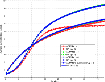
Figure 3: Differential feedback signaling with $q$-bit quantization.

VII User Admission

Overloaded initialization, in the sense that there are more active spatial data streams than available DoF, has been proposed in various publications as an efficient user admission design [2]. As a result of the transceiver iteration, the excess streams will be dropped, i.e., the corresponding beamformers will get zero power [2].

For static channels, the overloaded initialization can be used as a low complexity user allocation approach, particularly, for complex systems with a large number of users. This is not particularly convenient for time correlated channel models, where the channel conditions change in time. In such cases, it is more beneficial to dynamically change the user allocation to better reflect the changing channel conditions. However, reintroducing the dropped users is difficult as the priority weight factors of the reintroduced users should be proportional to the active users. Furthermore, once the spatial compatibility of the active streams is close to a local optima, it is difficult to reintroduce a stream to the system in such a way that the reintroduced streams potentially improve performance of the existing setup. In this case, it is likely that the reintroduced streams will be dropped, due to the spatial incompatibility.

To overcome the degraded beamformer compatibility in time correlated channels, we propose beamformer reinitialization after a given number of iterations. This effectively performs periodic user selection. The reinitialization has a significant impact on the system performance and has been numerically evaluated in Section VIII.

VII-A Varying beamformer signaling length

We can exploit the fact that the performance loss is caused by insufficient beamformer convergence. A straightforward approach is to make the beamformer signaling part of each frame longer. This gives more time for the beamformers to converge. However, this also increases the signaling overhead and, which may become excessive for the later iterations as the beamformers have already sufficiently converged and user selection has occurred.

We propose a varying length beamformer signaling among the frames, where the beamformer signaling interval is longer after each reinitialization point and shorter for the subsequent frames. This improves the inherent trade-off between the signaling overhead and beamformer convergence. This scheme has been illustrated in Fig. 4, where the number of signaling iterations is fixed to $\beta=10$ after each reinitialization frame and to $\beta=3$ for all the other frames. Varying the signaling lengths allows the algorithm to achieve most of the performance during the first frame while having most of the performance penalty in duration of one frame. This penalty is compensated during the subsequent frames with less beamformer signaling iterations.

Figure 4: An example of varying number beamformer signaling iterations with respect to the user reinitialization index.

VII-B Delayed beamformer indexing

Having a varying length beamformer training iterations depending on the frame index may require excessive planning in smaller (femto sized) systems as the TDD frame structure has to be globally identical in order to assure limited pilot signal contamination by the interfering transmissions. To this end, we propose a more flexible alternative method to improve the diminished system performance after each beamformer reinitialization.

For reasonably slow fading channels, we may assume that the changes in the channels between two consecutive frames is not overly drastic. Thus, the performance decrease for fixed beamformers between two frames is only minor. This assumption may be exploited with the beamformer reinitialization by delaying the beamformer indexing in the sense that, as the trained transmit/receive beamformers are reinitialized, the beamformers before the reinitialization are used for the actual data transmission until the trained beamformers have converged to sufficiently high performance.

Note that the receive beamformers can be always assumed to be up-to-date as the active transmit beamformers can be estimated directly from the demodulation pilots (see Fig. 2). Here, $\mathbf{m}(t_{i})$ denotes the active beamformers generated in the frame $t_{i}$. By delaying the beamformers for one iteration after the reset, the degradation in the achievable rate is significantly reduced. On the second frame after the reinitialization, the active beamformers have already converged to overcome most of the negative impact from the beamformer reset and can be switched as the active beamformers for the actual data transmission.

Figure 5: An illustration of delayed transmit beamformer indexing.

In the end, this technique utilizes two sets of beamformers. First set consists of the beamformers that are being trained and iteratively exchanged among the interfering transmitters using the bi-directional signaling portion of the frame structure. The second set of beamformers are the ones that used in the current frame to actually transmit the data.

VIII Numerical Examples

The simulations are carried out using a 7-cell wrap around model, where the distance between the BS is $600\text{m}$. The path loss exponent for the user terminals is fixed to $3$. The number of transmit and receive antennas are set to $N_{\text{T}}=4$ and $N_{\text{R}}=2$, respectively. There are $K_{b}=7$ user terminals that are evenly distributed on the cell edge around each BS. In total, there are $K=BK_{b}=49$ users in the network. We assume full cooperation, i.e., all users are coherently served by every BS in the system. In practice, practical constraints such as pilot contamination will limit the number of active users per-BS. The number of active spatial stream per users is limited to one. The simulation environment is illustrated in Fig. 6.

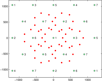
Figure 6: Base station and cell edge user terminal deployment in 7-cell wrap around model with $K_{b}=7$ in each cell.

The SNR is defined on the cell edge from the closest BS $b$, i.e, $\text{SNR}=\frac{g_{b,k}P_{b}}{\sigma_{k}^{2}}$, where $g_{b,k}$ denotes the corresponding path loss. The channels are generated with Jakes’ Doppler spectrum model. The channel coherence time is defined by normalized user terminal velocity $t_{\text{S}}f_{\text{D}}$, where $t_{\text{S}}$ and $f_{\text{D}}$ are the backhaul signaling rate and the maximum Doppler shift, respectively. Simulations are performed for two user velocity scenarios $t_{\text{S}}f_{\text{D}}=0.01$ and $t_{\text{S}}f_{\text{D}}=0.025$ that correspond to user velocities of $2.7$ km/h and $6.9$ km/h, respectively. The block fading model assumes that the channels remain constant during the transmission of each frame, and the changes occur in-between the frames. If not mentioned otherwise, the ADMM simulations are done with $\rho=3$ and BR simulations are performed with $\alpha=0.5$. Summary of the simulation parameters is listed in Table II.

TABLE II: Simulation parameters.

Parameter	Value
Number of UE ($K$)	$49$
Number of cells ($B$)	$7$
Number of UE per cell	$7$
BS antennas ($N_{\text{T}}$)	$2$
UE antennas ($N_{\text{R}}$)	$2$
Distance between adjacent BS	$600$ m
The path loss exponent	$3$
Signaling rate ($t_{S}$)	$2$ ms
Carrier frequency	$2$ GHz
UE velocities	$0$ km/h, $2.7$ km/h and $6.9$ km/h

The bi-directional signaling overhead is considered using coefficient $\gamma\in[0,1]$, so that the achievable rate is defined as $(1-\gamma)R$. The overhead coefficient $\gamma$ defines the fraction of the frame length, which is reserved for the signaling sequence. The number of UL/DL signaling iterations is denoted by BIT (bi-directional iterations). By this notation, the complete frame length is $2\gamma^{-1}\text{BIT}$. We assume that the UE feedback channels are slow in the sense that the stream specific weights $w_{k,l}\ \forall\ (k,l)$ can be exchanged only once per frame. That is, the bidirectional iteration, within a frame, only involves TDD based beamformer signaling.

VIII-A Stream Specific Estimation Methods

The proposed SSE methods from Section IV are compared in Fig. 7. The asymptotic performance of all of the proposed designs are comparable and the differences in performance are mostly related to the rate of convergence. It can be seen that the ADMM design provides the fastest initial convergence. However, the performance becomes comparable to the BR method after few initial iterations. The SG approach has slower rate of convergence. However, the step size normalization does help. When taking into account the lower complexity, the SG approach can be seen to be a viable alternative to the more complex decentralized methods.

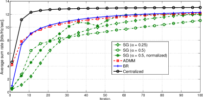
Figure 7: Average achievable sum rate per BS in static channel.

In Fig. 8, the SSE methods are compared using time correlated channels. The dashed lines show the performance for UE speed of $2.7$ km/h and the solid lines show the performance with UE speed of $6.9$ km/h. The time correlated indicates similar behavior to the static channel. The rate of convergence of the ADMM method is faster in the beginning, which results in good performance for the first, few iterations. However, the reduced rate of convergence for the later iterations, results in somewhat diminished capability to follow the channel changes. The BR design performs the best in the later phase. On the other hand, the SG based beamforming provides competitive performance, considering the greatly reduced computational complexity.

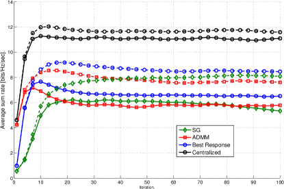
Figure 8: Average achievable sum rate per BS in time correlated channels with UE speeds $2.7$ km/h (dashed) and $6.9$ km/h (solid).

VIII-B Direct Estimation

Fig. 9 demonstrates the performance of the centralized DE and SSE as the length of the pilot training sequence is varied. Here, the SSE beamformer design is done with the same pilots as the DE, only ignoring the pilot cross-talk and estimation error. It is easy to confirm that DE has clear advantage, when the pilot contamination levels are high. On the other hand, it should be noted that with sufficiently long pilot sequences the pilots can be made fully orthogonal, which reduces the performance gap with large pilot lengths.

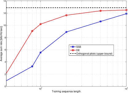
Figure 9: Centralized DE behavior for varying training sequence lengths in constant channel.

The impact of the pilot sequence length on the decentralized DE processing is shown in Fig.10. It DE-ADMM and DE-BR methods have clearly comparable performance. While the DE-SG design requires larger pilot lengths, to achieve comparable asymptotic performance. For the DE-SG, momentum and step-size normalization can be seen to significantly improve the performance.

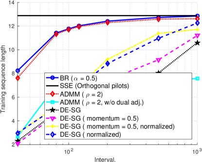
Figure 10: Comparison of the decentralized DE methods with varying training sequence lengths in constant channel.

Figs. 11 and 11 show the performance of the centralized DE in time correlated channel with UE speeds $2.7$km/h and $6.9$km/h, respectively. The time correlated behaviour is similar to the constant channel performance. As the UE speed grows, the gap between the SSE and DE methods diminishes. This is due the fact that both methods have similarly out-of-date CSI and beamforming gain is no longer available.

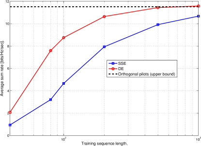
Figure 11: DE behavior for varying training sequence lengths in time correlated channels with UE speed $2.7$ km/h.

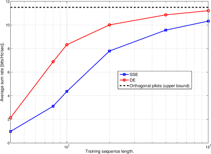
Figure 12: DE-BR behavior for varying training sequence lengths in time correlated channels with UE speed $6.9$ km/h.

VIII-B1 DE-BR

From Fig. 13, it is evident that the BR will convergence to match the SSE performance, given long enough pilot sequences. Also, the significance of the pilot sequence length diminishes when the pilot sequence length grows larger than the number of interfering streams in the system, i.e., when $S$ grows larger than $49$.

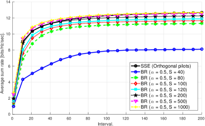
Figure 13: DE-BR performance for varying training sequence lengths in constant channel.

The behavior of the DE-BR in time correlated channels are shown in Figs. 14 and 12. Here, the orthogonal pilot allocation upper bound is generated by using the BR method from IV-A. Again, we can see that as $S$ grows larger that there are interfering stream, the difference in performance is neglectible.

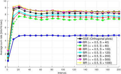
Figure 14: DE-BR behavior for varying training sequence lengths in time correlated channels with UE speed $2.7$ km/h.

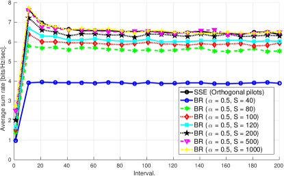
Figure 15: DE-BR behavior for varying training sequence lengths in time correlated channels with UE speed $6.9$ km/h.

VIII-B2 DE-ADMM

When not otherwise stated the dual updates 64 are done using $\beta=1/\rho$. Fig. 16 demonstrates the DE-ADMM method convergence behavior. Performance in time correlated channels is shown in Figs. 17 and 18. The performance can be seen to be nearly identical to the DE-ADMM approach.

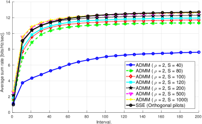
Figure 16: DE-ADMM performance for varying training sequence lengths in constant channel.

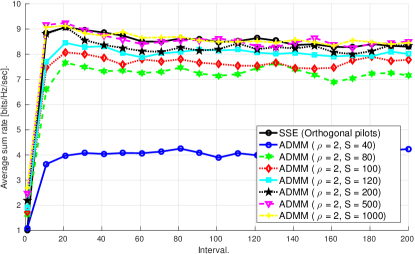
Figure 17: DE-ADMM behavior for varying training sequence lengths in time correlated channels with UE speed $2.7$ km/h.

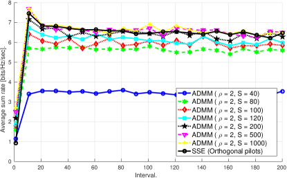
Figure 18: DE-ADMM behavior for varying training sequence lengths in time correlated channels with UE speed $6.9$ km/h.

VIII-B3 DE-SG

Fig. 19 shows the performance of the decentralized DE-SG method. The DE-SG design can be seen to approach the performance of SSE design without pilot contamination as the training sequence length becomes sufficiently large.

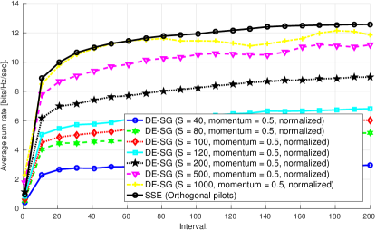
Figure 19: DE-SG performance for varying training sequence lengths in constant channel.

DE-SG performance in time correlated channels is show in Fig. 20 and Fig. 21. In comparison to DE-BR and DE-ADMM, we can see that the SG is more sensitive to the pilot sequence length.

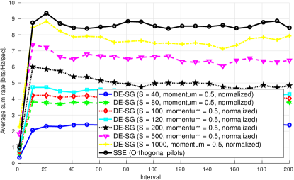
Figure 20: DE-SG behavior for varying training sequence lengths in time correlated channels with UE speed $2.7$ km/h.

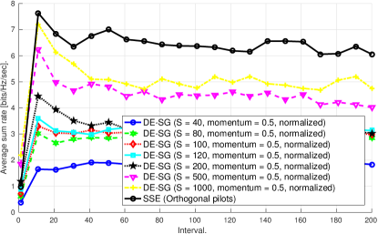
Figure 21: DE-SG behavior for varying training sequence lengths in time correlated channels with UE speed $6.9$ km/h.

VIII-C User Admission

For the user admission, we lower the number of transmit antennas to $N_{\text{T}}=2$. This makes the system overloaded in the sense that there are more initialized beamformers than there are available DoF. There are $K=49$ initialized streams, while there are only $BN_{\text{T}}=28$ degrees-of-freedom. As discussed in Section VII, the excess streams get dropped during the beamformer iteration, which effectively means that user selection is performed. The performance of the user admission methods is evaluated with the BR design.

In Fig. 22 and 23, the system performance is shown in time correlated channels. Before each reinitialization, the beamformers are stored for the delayed indexing. Clearly, as the channels change, the initial user selection becomes inefficient and periodically initializing the beamformers allows the user allocation to better adjust to the changing channel conditions. The delayed indexing significantly improves the performance while retraining the beamformers. The bi-directional signaling can be seen to improve the stability of the algorithm behavior as well as the convergence properties. As the channel changes more aggressively the performance of the delayed indexing beamformers is diminished.

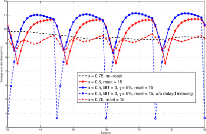
Figure 22: Average system performance using periodic reset with UE speed $2.7$ km/h and SNR $=20$dB.

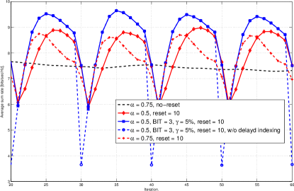
Figure 23: Average system performance using periodic reset with UE speed $6.9$ km/h and SNR $=20$dB.

From Fig. 24, we can observe two types of benefits from the varying length signaling iterations. First, the performance degradation after the beamformer reinitialization is reduced. Secondly, the performance of the following iterations is improved. This is due to the benefit of letting the beamformers convergence for 10 iterations during the first frame after the reinitialization, which results in higher improved spatial compatibility between the transmissions on the following iterations and leads to improved system performance.

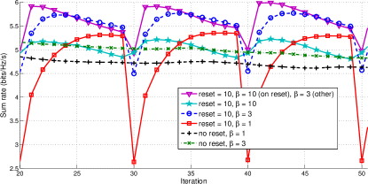
Figure 24: Average sum rate behavior of the varying length beamformer signaling with 10 frame reset interval, UE speed $6.9km/h$ and $\gamma=0.02$.

IX Conclusions

We have proposed decentralized transceiver designs for coherent CoMP WSRMax. We considered orthogonal pilot resource allocation without pilot estimation noise and scenarios with non-orthogonal and noise pilots. Along with low complexity and signaling overhead transceiver designs, we provided novel techniques for user admission and beamformer training. Numerical results indicated that our designs provide good performance and stability even with time correlated channel conditions.

Appendix A Simplification of (23)

To simplify expression (23), we can eliminate the auxiliary variables $s_{k,l,b,i,z}\ \forall\ (k,l,b,i,z)$ [36]. By solving the individual $s_{k,l,b,i,z}$ from (23), while keeping the other variables fixed, we have

$$s_{k,l,b,i,z}=a_{k,l,b,i,z}^{(n)}+\frac{\bar{s}_{k,l,i,z}}{|\mathcal{B}_{i}|}-\frac{\bar{\lambda}_{k,l,i,z}^{(n)}}{|\mathcal{B}_{i}|}-\frac{r_{k,l,i,z}}{|\mathcal{B}_{i}|}\text{,}$$ (72)

where $\bar{\lambda}_{k,l,i,z}^{(n)}=\sum_{g\in\mathcal{B}_{i}}\lambda_{k,l,g,i,z}^{(n)}$, $a_{k,l,b,i,z}^{(n)}=\lambda_{k,l,b,i,z}^{(n)}+\mathbf{u}_{k,l}^{\mbox{\scriptsize H}}\mathbf{H}_{b,k}\mathbf{m}_{b,i,z}$ and $r_{k,l,i,z}=\sum_{g\in\mathcal{B}_{i}}\sqrt{w_{k,l}}\mathbf{u}_{k,l}^{\mbox{\scriptsize H}}\mathbf{H}_{j,k}\mathbf{m}_{g,i,z}$. It is easy to see that (72) minimizes (23) and satisfies (21), as derived in the following

$$\begin{array}[]{rl}\displaystyle\sum_{b\in\mathcal{B}_{i}}s_{k,l,b,i,z}=& \displaystyle\sum_{b\in\mathcal{B}_{i}}a_{k,l,b,i,z}^{(n)}+\bar{s}_{k,l,i,z}-\bar{\lambda}_{k,l,i,z}^{(n)}-r_{k,l,i,z}\\ =&\displaystyle\bar{s}_{k,l,i,z}\text{.}\end{array}$$ (73)

When we substitute each $s_{k,l,b,i,z}$ in (23) with (72), the consensus constraints must hold as shown in (73). On the other hand, the penalty terms (20) reduce to

$$\begin{array}[]{rl}\displaystyle\Theta_{k,l}&=\displaystyle\sum_{i=1}^{K}\sum_{z=1}^{L_{i}}\sum_{b\in\mathcal{B}_{i}}\frac{\rho}{2}|\frac{r_{k,l,i,z}}{|\mathcal{B}_{i}|}-\frac{\bar{s}_{k,l,i,z}}{|\mathcal{B}_{i}|}+\frac{\bar{\lambda}_{k,l,i,z}^{(n)}}{|\mathcal{B}_{i}|}|^{2}\\ \displaystyle\hfil&=\displaystyle\sum_{i=1}^{K}\sum_{z=1}^{L_{i}}\sum_{b\in\mathcal{B}_{i}}\frac{\rho}{2|\mathcal{B}_{i}|}|r_{k,l,i,z}-\bar{s}_{k,l,i,z}+\bar{\lambda}_{k,l,i,z}^{(n)}|^{2}\text{.}\end{array}$$ (74)

Since, $\rho$ is an adjustable penalty constant, we can include the JP set sizes into it and, thus get

$$\Theta_{k,l}=\sum_{i=1}^{K}\sum_{z=1}^{L_{i}}\sum_{b\in\mathcal{B}_{i}}\frac{\rho}{2}|r_{k,l,i,z}-\bar{s}_{k,l,i,z}+\bar{\lambda}_{k,l,i,z}^{(n)}|^{2}\text{.}$$ (75)

Now, the same substitution for the dual update (24) and having the JP set sizes included into $\rho$, we have

$$\begin{array}[]{rl}\displaystyle\lambda_{k,l,b,i,z}^{(n+1)}&=\displaystyle\lambda_{k,l,b,i,z}^{(n)}+\sqrt{w_{k,l}}\mathbf{u}_{k,l}^{\mbox{\scriptsize H}}\mathbf{H}_{j,k}\mathbf{m}_{b,i,z}^{(n+1)}-s_{k,l,b,i,z}^{(n+1)}\\ &=\displaystyle\bar{s}_{k,l,i,z}-\bar{\lambda}_{k,l,i,z}^{(n)}-r_{k,l,i,z}\text{.}\end{array}$$ (76)

Since (76) does not depend on $b$, dual variables $\lambda_{k,l,b,i,z}\ \forall(k,l,i,z)$ are equivalent for all $b\in\mathcal{B}_{i}$. Thus, we can combine all dual variables for each $(k,l,i,z)$ and have (26).

References

- [1] E. Dahlman, S. Parkvall, and J. Sköld, 4G LTE / LTE-Advanced for Mobile Broadband. Academic Press, 2011.
- [2] Q. Shi, M. Razaviyayn, Z.-Q. Luo, and C. He, “An iteratively weighted MMSE approach to distributed sum-utility maximization for a MIMO interfering broadcast channel,” IEEE Trans. Signal Processing, vol. 59, no. 9, pp. 4331–4340, Sep. 2011.
- [3] P. Komulainen, A. Tolli, and M. Juntti, “Effective CSI Signaling and Decentralized Beam Coordination in TDD Multi-Cell MIMO Systems,” IEEE Trans. Signal Processing, vol. 61, no. 9, pp. 2204–2218, 2013.
- [4] A. Tölli, H. Pennanen, and P. Komulainen, “Decentralized minimum power multi-cell beamforming with limited backhaul signaling,” IEEE Trans. Wireless Commun., vol. 10, no. 2, pp. 570–580, Feb. 2011.
- [5] T. Bogale and L. Vandendorpe, “Weighted sum rate optimization for downlink multiuser MIMO coordinated base station systems: Centralized and distributed algorithms,” IEEE Trans. Signal Processing, Dec. 2011.
- [6] H. Pennanen, A. Tolli, and M. Latva-aho, “Decentralized Coordinated Downlink Beamforming via Primal Decomposition,” IEEE Signal Processing Lett., vol. 18, no. 11, pp. 647–650, Nov. 2011.
- [7] D. Gesbert, S. Hanly, H. Huang, S. Shamai Shitz, O. Simeone, and W. Yu, “Multi-Cell MIMO Cooperative Networks: A New Look at Interference,” IEEE J. Select. Areas Commun., vol. 28, no. 9, pp. 1380–1408, 2010.
- [8] S. Zhou, J. Gong, and Z. Niu, “Distributed Adaptation of Quantized Feedback for Downlink Network MIMO Systems,” IEEE Trans. Wireless Commun., vol. 10, no. 1, pp. 61–67, Jan. 2011.
- [9] D. Lee, H. Seo, B. Clerckx, E. Hardouin, D. Mazzarese, S. Nagata, and K. Sayana, “Coordinated multipoint transmission and reception in LTE-Advanced: deployment scenarios and operational challenges,” IEEE Commun. Mag., vol. 50, no. 2, pp. 148–155, Feb. 2012.
- [10] C. L. I, C. Rowell, S. Han, Z. Xu, G. Li, and Z. Pan, “Toward green and soft: a 5G perspective,” IEEE Commun. Mag., vol. 52, no. 2, pp. 66–73, Feb. 2014.
- [11] J. Zhang and J. Andrews, “Adaptive spatial intercell interference cancellation in multicell wireless networks,” IEEE J. Select. Areas Commun., vol. 28, no. 9, pp. 1455–1468, 2010.
- [12] S. Han, C. Yang, G. Wang, D. Zhu, and M. Lei, “Coordinated Multi-Point Transmission Strategies for TDD Systems with Non-Ideal Channel Reciprocity,” IEEE Trans. Commun., vol. 61, no. 10, pp. 4256–4270, Oct. 2013.
- [13] T. M. Kim, F. Sun, and A. Paulraj, “Low-Complexity MMSE Precoding for Coordinated Multipoint With Per-Antenna Power Constraint,” IEEE Signal Processing Lett., vol. 20, no. 4, pp. 395–398, 2013.
- [14] S. Shi, M. Schubert, and H. Boche, “Rate optimization for multiuser mimo systems with linear processing,” IEEE Trans. Signal Processing, vol. 56, no. 8, pp. 4020–4030, Aug. 2008.
- [15] M. Codreanu, A. Tölli, M. Juntti, and M. Latva-aho, “Joint design of Tx-Rx beamformers in MIMO downlink channel,” IEEE Trans. Signal Processing, vol. 55, no. 9, pp. 4639–4655, Sep. 2007.
- [16] S. S. Christensen, R. Agarwal, E. Carvalho, and J. Cioffi, “Weighted sum-rate maximization using weighted MMSE for MIMO-BC beamforming design,” IEEE Trans. Wireless Commun., vol. 7, no. 12, pp. 4792–4799, Dec. 2008.
- [17] G. Scutari, F. Facchinei, P. Song, D. Palomar, and J.-S. Pang, “Decomposition by partial linearization: Parallel optimization of multi-agent systems,” IEEE Trans. Signal Processing, vol. 62, no. 3, pp. 641–656, Feb. 2014.
- [18] J. Kaleva, A. Tölli, and M. Juntti, “Decentralized sum rate maximization with QoS constraints for interfering broadcast channel via successive convex approximation,” IEEE Trans. Signal Processing, vol. 64, no. 11, pp. 2788–2802, Jun. 2016.
- [19] M. Hong, R. Sun, H. Baligh, and Z.-Q. Luo, “Joint base station clustering and beamformer design for partial coordinated transmission in heterogeneous networks,” IEEE J. Select. Areas Commun., vol. 31, no. 2, pp. 226–240, Feb. 2013.
- [20] S. H. Park, O. Simeone, O. Sahin, and S. Shamai, “Joint precoding and multivariate backhaul compression for the downlink of cloud radio access networks,” IEEE Trans. Signal Processing, vol. 61, no. 22, pp. 5646–5658, Nov. 2013.
- [21] B. Dai and W. Yu, “Energy efficiency of downlink transmission strategies for cloud radio access networks,” IEEE J. Select. Areas Commun., vol. 34, no. 4, pp. 1037–1050, Apr. 2016.
- [22] F. Zhuang and V. Lau, “Backhaul limited asymmetric cooperation for MIMO cellular networks via semidefinite relaxation,” IEEE Trans. Signal Processing, vol. 62, no. 3, pp. 684–693, Feb. 2014.
- [23] W.-C. Liao, M. Hong, Y.-F. Liu, and Z.-Q. Luo, “Base station activation and linear transceiver design for optimal resource management in heterogeneous networks,” IEEE Trans. Signal Processing, vol. 62, no. 15, pp. 3939–3952, Aug. 2014.
- [24] J. Kaleva, M. Bande, A. Tölli, M. Juntti, and V. V. Veeravalli, “Sum Rate Maximizing Joint Processing with Limited Backhaul and Tree Topology Constraints,” in Proc. IEEE Works. on Sign. Proc. Adv. in Wirel. Comms., Edinburgh, UK, Jul. 2016.
- [25] S. H. Park, O. Simeone, O. Sahin, and S. Shamai, “Inter-cluster design of precoding and fronthaul compression for cloud radio access networks,” IEEE Commun. Lett., vol. 3, no. 4, pp. 369–372, Aug. 2014.
- [26] S. H. Park, O. Simeone, O. Sahin, and S. S. Shitz, “Fronthaul compression for cloud radio access networks: Signal processing advances inspired by network information theory,” IEEE Signal Processing Mag., vol. 31, no. 6, pp. 69–79, Nov. 2014.
- [27] C. Shen, T.-H. Chang, K.-Y. Wang, Z. Qiu, and C.-Y. Chi, “Distributed robust multicell coordinated beamforming with imperfect CSI: An ADMM approach,” IEEE Trans. Signal Processing, vol. 60, no. 6, pp. 2988–3003, Jun. 2012.
- [28] D. Kim, O.-S. Shin, I. Sohn, and K. B. Lee, “Channel Feedback Optimization for Network MIMO Systems,” IEEE Trans. Veh. Technol., vol. 61, no. 7, pp. 3315–3321, Sep. 2012.
- [29] D. Jaramillo-Ramírez, M. Kountouris, and E. Hardouin, “Coordinated multi-point transmission with imperfect CSI and other-cell interference,” IEEE Trans. Wireless Commun., vol. 14, no. 4, pp. 1882–1896, Apr. 2015.
- [30] J. Jose, A. Ashikhmin, T. L. Marzetta, and S. Vishwanath, “Pilot contamination and precoding in multi-cell tdd systems,” vol. 10, no. 8, pp. 2640–2651, Aug. 2011.
- [31] C. Shi, R. Berry, and M. Honig, “Bi-directional training for adaptive beamforming and power control in interference networks,” IEEE Trans. Signal Processing, vol. 62, no. 3, pp. 607–618, Feb. 2014.
- [32] M. Xu, D. Guo, and M. L. Honig, “Distributed bi-directional training of nonlinear precoders and receivers in cellular networks,” IEEE Trans. Signal Processing, vol. 63, no. 21, pp. 5597–5608, Nov. 2015.
- [33] J. Kaleva, R. Berry, M. Honig, A. Tolli, and M. Juntti, “Decentralized sum MSE minimization for coordinated multi-point transmission,” in Proc. IEEE Int. Conf. Acoust., Speech, Signal Processing, May 2014, pp. 469–473.
- [34] Z. Luo and S. Zhang, “Dynamic spectrum management: Complexity and duality,” IEEE J. Select. Areas Commun., vol. 2, no. 1, pp. 57–73, Feb. 2008.
- [35] S. Boyd and L. Vandenberghe, Convex Optimization. Cambridge, UK: Cambridge University Press, 2004.
- [36] S. Boyd, N. Parikh, E. Chu, B. Peleato, and J. Eckstein, “Distributed optimization and statistical learning via the alternating direction method of multipliers,” Foundations and Trends in Machine Learning, vol. 3, no. 1, pp. 1–122, 2010.
- [37] S. Boyd, “Primal and dual decomposition,” 2007, [Online]. Available: http://www.stanford.edu/class/ee364b/lectures/decomposition_slides.pdf.
- [38] Z. Q. Luo, T. N. Davidson, G. Giannakis, and K. M. Wong, “Transceiver optimization for block-based multiple access through ISI channels,” IEEE Trans. Signal Processing, vol. 52, no. 4, pp. 1037–1052, Apr. 2004.
- [39] M. Hong, Z.-Q. Luo, and M. Razaviyayn, “Convergence Analysis of Alternating Direction Method of Multipliers for a Family of Nonconvex Problems,” ArXiv e-prints, Oct. 2014.
- [40] S. Haykin, Adaptive Filter Theory, 3rd ed. Upper Saddle River, NJ, USA: Prentice Hall, 1996.