Emergence of chaos in a viscous solution of rods

Abstract

It is shown that the addition of small amounts of microscopic rods in a viscous fluid at low Reynolds number causes a significant increase of the flow resistance. Numerical simulations of the dynamics of the solution reveal that this phenomenon is associated to a transition from laminar to chaotic flow. Polymer stresses give rise to flow instabilities which, in turn, perturb the alignment of the rods. This coupled dynamics results in the activation of a wide range of scales, which enhances the mixing efficiency of viscous flows.

In a laminar flow the dispersion of substances occurs by molecular diffusion, which operates on extremely long time scales. Various strategies have therefore been developed, particularly in microfluidic applications, to accelerate mixing and dispersion at low fluid inertia SQ05 ; OW04 ; SSA04 . The available strategies are commonly divided into two classes, passive or active, according to whether the desired effect is obtained through the specific geometry of the flow or through an oscillatory forcing within the fluid SSA04 . An alternative method for improving the mixing properties of low-Reynolds-number flows was proposed by Groisman and Steinberg GS01 and consists in adding elastic polymers to the fluid. If the inertia of the fluid is low but the elasticity of polymers is large enough, elastic stresses give rise to instabilities that ultimately generate a chaotic regime known as “elastic turbulence” GS00 . In this regime the velocity field, although remaining smooth in space, becomes chaotic and develops a power-law energy spectrum, which enhances the mixing properties of the flow. While the use of elastic turbulence in microfluidics is now well established BSBGS04 ; JV11 ; PBCS12 ; TCT15 ; AWDP16 , new potential applications have recently emerged, namely in oil extraction from porous rocks Clarke16 .

In this Letter we propose a novel mechanism for generating chaotic flows at low Reynolds numbers that does not rely on elasticity. It is based on the addition of rigid rodlike polymers. At high Reynolds numbers, elastic- and rigid-polymer solutions exhibit remarkably similar macroscopic behavior (e.g., Refs. VSW97 ; PDDS04 ; BCLLP05 ; G08 ). In both cases the turbulent drag is considerably reduced compared to that of the solvent alone. In particular, when either type of polymer is added in sufficiently high concentrations to a turbulent channel flow of a Newtonian fluid, the velocity profile continues to depend logarithmically on the distance from the walls of the channel, but the mean velocity increases to a value known as maximum-drag-reduction asymptote. Here we study whether or not the similarity between elastic- and rigid-polymer solutions carries over to the low-Reynolds-number regime, i.e whether or not the addition of rigid polymers originates a regime similar to elastic turbulence.

We consider a dilute solution of inertialess rodlike polymers. The polymer phase is described by the symmetric unit-trace tensor field $\mathcal{R}(\bm{x},t)=\overline{n_{i}n_{j}}$, where $\bm{n}$ is the orientation of an individual polymer and the average is taken over the polymers contained in a volume element at position $\bm{x}$ at time $t$. The coupled evolution of $\mathcal{R}(\bm{x},t)$ and the incompressible velocity field $\bm{u}(\bm{x},t)$ is given by the following equations DE88 ; PLB08 (summation over repeated indices is implied):

$$\partial_{t}{u_{i}}+{u_{k}}\partial_{k}{u_{i}} =-\partial_{i}p+\nu\partial^{2}{u_{i}}+\partial_{k}{\sigma_{ik}}+{f_{i}}\,,$$ (1a)

$$\partial_{t}{\mathcal{R}_{ij}}+{u_{j}}\partial_{j}{\mathcal{R}_{ij}} =(\partial_{k}{u_{i}}){\mathcal{R}_{kj}}+{\mathcal{R}_{ik}}(\partial_{k}{u_{j}})-$$

$$\hskip 28.45274pt2\mathcal{R}_{ij}(\partial_{l}u_{k})\mathcal{R}_{kl},$$ (1b)

where $\partial_{k}=\partial/\partial x_{k}$, $p(\bm{x},t)$ is pressure, $\nu$ is the kinematic viscosity of the fluid, and $\bm{f}(\bm{x},t)$ is the body-force which sustains the flow. The polymer stress tensor takes the form $\sigma_{ij}=6\nu\eta_{\mathrm{p}}\mathcal{R}_{ij}(\partial_{l}u_{k})\mathcal{R}_{kl}$ DE88 . The intensity of the polymer feedback on the flow is determined by the polymer concentration, which is proportional to $\eta_{\mathrm{p}}$. This expression for the polymer stress tensor is based on a quadratic approximation proposed by Doi and Edwards DE88 . More sophisticated closures have been employed in the literature (see, e.g., Ref. MHJS11 and references therein); here we focus on the simplest model of rodlike-polymer solution that may display instabilities at low Reynolds number. In addition, we disregard Brownian rotations assuming that the orientation of polymers is mainly determined by the velocity gradients.

For large values of the Reynolds number, the system described by Eqs. (1) has been shown to reproduce the main features of drag reduction in turbulent solutions of rodlike polymers BCLLP05 ; BCDP08 ; PLB08 ; ABKLLP08 . Here we study the same system at small values of the Reynolds number. Equations (1) are solved over a two-dimensional $2\pi$-periodic box and $\bm{f}$ is taken to be the Kolmogorov force $\bm{f}(\bm{x})=(0,F\sin(x/L))$. For $\eta_{\mathrm{p}}=0$ the flow has the laminar solution $\bm{u}=(0,U_{0}\sin(x/L))$ with $U_{0}=FL^{2}/\nu$, which becomes unstable when the Reynolds number $\mathrm{Re}=U_{0}L/\nu$ exceeds the critical value $\mathrm{Re}_{\mathrm{c}}=\sqrt{2}$ and eventually turbulent when $\mathrm{Re}$ is increased further (e.g., Ref. MB14 ). Even in the turbulent regime, the mean flow has the sinusoidal form $\langle\bm{u}\rangle=(0,U\sin(x/L))$, where $\langle\bm{\cdot}\rangle$ denotes an average over the variable $y$ and over time. The Kolmogorov force has been previously used in the context of non-Newtonian fluid mechanics to study turbulent drag reduction BCM05 , the formation of low-$\mathrm{Re}$ instabilities in viscoelastic BCMPV05 ; BBCMPV07 and rheopectic fluids BMP13 , and elastic turbulence BBBCM08 ; BB10 .

Numerical simulations of Eqs. (1) are performed by using a dealiased pseudospectral method with $1024^{2}$ gridpoints. The time-integration uses a fourth-order Runge-Kutta scheme with implicit integration of the linear dissipative terms. The parameters of the simulations are set to keep $\mathrm{Re}=1$ fixed below $\mathrm{Re}_{\mathrm{c}}$ in the absence of polymer feedback ($\eta_{\mathrm{p}}=0$). The viscosity is set to $\nu=1$, the length scale of the forcing is either $L=1/4$ or $L=1/8$, and its amplitude is $F=\nu^{2}/L^{3}$. The feedback coefficient is varied from $\eta_{\mathrm{p}}=1$ to $\eta_{\mathrm{p}}=5$. The stiffness of the equations increases with $\eta_{\mathrm{p}}$, limiting the accessible range of parameters.

Initially the flow is a weak perturbation of the $\eta_{\mathrm{p}}=0$ stable solution, while the components of $\mathcal{R}$ are randomly distributed. When the feedback of the polymers is absent ($\eta_{\mathrm{p}}=0$) the initial perturbation decays and the polymers align with the direction of the mean shear flow. Conversely, at large $\eta_{\mathrm{p}}$ the flow is strongly modified by the presence of the rods. The streamlines wiggle over time and thin filaments appear in the vorticity field $\omega=|\bm{\nabla}\times\bm{u}|$ (see Fig. 1, left panel). These filaments correspond to appreciable localized perturbations of the tensor $\mathcal{R}$ away from the laminar fixed point (Fig. 1, right panel) and are due to the rods being unaligned with the shear direction. Notably, we find that the mean flow, obtained by means of long time averages, maintains the sinusoidal form $\langle\bm{u}\rangle=(0,U\sin(x/L))$ also in the presence of strong polymer feedback (Fig. 2).

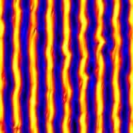
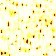
Figure 1: Left: Snapshot of the vorticity field $\omega$ for $\eta_{\mathrm{p}}=3$ and $L=1/8$. Black (white) represents negative (positive) vorticity. Right: Snapshot of the component $\mathcal{R}_{11}$. White represents 0, black represents 1.

Figure 2: Mean velocity profiles for $L=1/8$ and concentrations $\eta_{\mathrm{p}}=1$ (solid), $\eta_{\mathrm{p}}=3$ (dotted), and $\eta_{\mathrm{p}}=5$ (dashed).

The time series of the kinetic energy in Fig. 3 show that, in the case of a low concentration ($\eta_{\mathrm{p}}=1$), the system repetitively attempts but fails to escape the laminar regime in a quasiperiodic manner. The amount of kinetic energy is initially close to that in the laminar regime. After some time, the solution dissipates a small fraction of kinetic energy but quickly relaxes back towards the laminar regime until it restarts this cyclic pattern. In contrast, for higher concentrations the kinetic energy is significantly reduced and, after an initial transient, fluctuates around a constant value. We have observed that different initial conditions for $\mathcal{R}$ may give rise to longer transients that involve a quasiperiodic sequence of activations and relaxations comparable to that observed for low values of $\eta_{\mathrm{p}}$. Nevertheless, the statistically steady state achieved at later times is independent of the peculiar choice of initial conditions.

Figure 3: The kinetic energy $\mathcal{E}$ for $L=1/8$ and concentrations $\eta_{\mathrm{p}}=1$ (top, solid), $\eta_{\mathrm{p}}=3$ (middle, dotted), and $\eta_{\mathrm{p}}=5$ (bottom, dashed) divided by the kinetic energy $\mathcal{E}_{0}=F^{2}L^{4}/2\nu^{2}$ corresponding to $\eta_{\mathrm{p}}=0$ and the same value of the force $F$.

The reduction of the kinetic energy of the flow at fixed intensity of the external force reveals that the presence of the rods causes an increase in the flow resistance. This effect can be quantified by the ratio of the actual mean power $P=FU/2$ provided by the external force and the power $P_{\mathrm{lam}}=F_{0}U/2$ that would be required to sustain a laminar mean flow with the same amplitude $U$ in the absence of polymers. In the latter case, the force required would be $F_{0}=\nu U/L^{2}$ and the corresponding mean power would be $P_{\mathrm{lam}}=F_{0}U/2=\nu U^{2}/2L^{2}$. Figure 4 shows the ratio

$$\dfrac{P}{P_{\mathrm{lam}}}=\dfrac{F}{F_{0}}=\dfrac{FL^{2}}{\nu U}$$ (2)

as a function of $\eta_{\mathrm{p}}$ and indicates that more power is required to sustain the same mean flow in solutions with higher concentrations.

Figure 4: The normalized mean injected power $P/P_{\mathrm{lam}}$ as a function of $\eta_{\mathrm{p}}$. Inset: The amplitudes of the stresses $\Pi_{r}$ (brown $\square$), $\Pi_{\nu}$ (blue ${\bullet}$), and $\Pi_{p}$ (red $\times$) divided by the amplitude of the total stress $\Pi_{\mathrm{tot}}$ for $L=1/8$ and different values of $\eta_{\mathrm{p}}$ (see Table 1).

The analysis of the momentum budget confirms that the increased resistance is due to an increase of the amount of stress due to the polymers. In the steady state the momentum budget can be obtained by averaging Eq. (1a) over $y$ and time:

$$\partial_{x}\Pi_{r}=\partial_{x}(\Pi_{\nu}+\Pi_{p})+f_{y},$$ (3)

where $\Pi_{r}=\langle u_{x}u_{y}\rangle$, $\Pi_{\nu}=\nu\partial_{x}\langle u_{y}\rangle$, and $\Pi_{p}=\langle\sigma_{xy}\rangle$ are the Reynolds, viscous, and polymer stress, respectively. Remarkably we find that these profiles remain sinusoidal as in the $\eta_{\mathrm{p}}=0$ case, namely $\Pi_{\mathrm{r}}=-S\cos(x/L)$, $\Pi_{\nu}=\nu UL^{-1}\cos(x/L)$, and $\Pi_{p}=\Sigma\cos(x/L)$. Equation (3) then yields the following relation between the amplitudes of the different contributions to the stress:

$$S+\dfrac{\nu U}{L}+\Sigma=FL.$$ (4)

These contributions are reported in Table 1 and they are shown in the inset of Fig. 4.

$\eta_{\mathrm{p}}$	$L$	$\Pi_{r}/\Pi_{\mathrm{tot}}$	$\Pi_{\nu}/\Pi_{\mathrm{tot}}$	$\Pi_{p}/\Pi_{\mathrm{tot}}$
1	1/8	0.001	0.996	0.004
2	1/8	0.004	0.887	0.110
3	1/4	0.005	0.787	0.209
3	1/8	0.005	0.795	0.200
4	1/8	0.007	0.710	0.284
5	1/8	0.006	0.647	0.347

Table 1: Amplitude of the stresses $\Pi_{r}$, $\Pi_{\nu}$, and $\Pi_{p}$ divided by the amplitude of the total stress $\Pi_{\mathrm{tot}}=\Pi_{r}+\Pi_{\nu}+\Pi_{p}$ for different values of $\eta_{\mathrm{p}}$ and $L$.

The results confirm that the polymer contribution to the total stress increases with $\eta_{\mathrm{p}}$, whereas that of the viscous stress decreases. The contribution of the Reynolds stress is extremely small (less than $10^{-2}$), which demonstrates that inertial effects remain negligible as $\eta_{\mathrm{p}}$ is increased. Figures 3 and 4 also suggest the presence of a threshold concentration for the appearance of fluctuations.

Further insight into the dynamics of the solution is gained by examining the energy balance in wave-number space.

Figure 5: The kinetic energy spectrum $E(k)$ for $L=1/4$, $\eta_{\mathrm{p}}=3$ (solid red) and $L=1/8$, $\eta_{\mathrm{p}}=5$ (dashed blue). The two black dotted segments represent $k^{-4}$ and $k^{-5}$. Inset: The unsigned kinetic-energy dissipation spectrum $2\nu k^{2}E(k)$ (magenta $+$) and the polymer energy transfer (solid black) for $L=1/4$ and $\eta_{\mathrm{p}}=3$.

For sufficiently large values of $\eta_{\mathrm{p}}$, the kinetic-energy spectrum behaves as a power law $E(k)\sim k^{-\alpha}$, where the exponent $\alpha$ depends both on the concentration and on the scale of the force and varies between $4$ and $5$ (Fig. 5). A wide range of scales is therefore activated, and this results to an enhancement of the mixing properties of the flow. Furthermore, the energy transfer due to the fluid inertia is negligible, and the dynamics is characterized by a scale-by-scale balance between the polymer energy transfer and viscous dissipation (inset of Fig. 5).

The regime described here has properties comparable to those of elastic turbulence in viscoelastic fluids, namely the flow resistance is increased with the addition of rods and the kinetic-energy spectrum displays a power-law steeper than $k^{-3}$. In addition the Reynolds stress and the energy transfer due to the fluid inertia are negligible; hence the emergence of chaos is entirely attributable to polymer stresses. Our study establishes an analogy between the behavior of viscoelastic fluids and that of solutions of rodlike polymers, similar to what is observed at high Reynolds number. These results therefore demonstrate that elasticity is not essential to generate a chaotic behavior at low Reynolds numbers and indicate an alternative mechanism to enhance mixing in microfluidic flows. This mechanism presumably has the advantage of being less affected by the degradation observed in elastic turbulence GS04 , since there are experimental evidences that the degradation due to large strains is weaker for rodlike polymers than for elastic polymers PAS13 .

Experimental studies aimed at investigating the phenomenon proposed in this Letter would be very interesting. Open questions concern the dependence of the mixing properties of rigid-polymer solutions on the type of force and on the boundary conditions. Additional insight into the dynamics of these polymeric fluids would also come from a stability analysis of system (1), in the spirit of the approach taken for the study of low-Reynolds-number instabilities in viscoelastic BCMPV05 ; BBCMPV07 and rheopectic BMP13 fluids. Finally, the orientation and rotation statistics of microscopic rods in turbulent flows has recently attracted a lot of attention PW11 ; PCTV12 ; GEM14 ; GVP14 ; VS17 ; it would be interesting to investigate the dynamics of individual rods in the flow regime studied here.

- (1) J.M. Ottino and S. Wiggins, Phil. Trans. R. Soc. A 362, 923 (2004).
- (2) H.A. Stone, A.D. Stroock, and A. Ajdari, Ann. Rev. Fluid Mech. 36, 381 (2004).
- (3) T.M. Squires and S.R. Quake, Rev. Mod. Phys. 77, 977 (2005).
- (4) A. Groisman and V. Steinberg, Nature 410, 905 (2001).
- (5) A. Groisman and V. Steinberg, Nature 405, 53 (2000).
- (6) T. Burghelea, E. Segre, I. Bar-Joseph, A. Groisman, and V. Steinberg, Phys. Rev. E 69, 066305 (2004).
- (7) Y. Jun and V. Steinberg, Phys. Rev. E 84, 056325 (2011).
- (8) R.J. Poole, B. Budhiraja, A.R. Cain, and P.A. Scott, J. Non-Newtonian Fluid Mech. 177-178, 15 (2012).
- (9) B. Traore, C. Castelain, and T. Burghelea, J. Non-Newtonian Fluid Mech. 223, 62 (2015).
- (10) W.M. Abed, R.D. Whalley, D.J.C. Dennis, and R.J. Poole, J. Non-Newtonian Fluid Mech. 231, 68 (2016).
- (11) A. Clarke, A.M. Howe, J. Mitchell, J. Staniland, and L.A. Hawkes, SPE Journal 21, 0675 (2016).
- (12) P.S. Virk, D.C. Sherman, and D.L. Wagger, AIChE J. 43, 3257 (1997).
- (13) J.S. Paschkewitz, Y. Dubief, C.D. Dimitropoulos, and E.S.G. Shaqfeh, J. Fluid Mech. 518, 281 (2004).
- (14) R. Benzi, E.S.C Ching, T.S. Lo, V.S. L’vov, and I. Procaccia, Phys. Rev. E 72, 016305 (2005).
- (15) J.J.J. Gillissen, Phys. Rev. E 78, 046311 (2008).
- (16) M. Doi and S.F. Edwards, The Theory of Polymer Dynamics. Oxford Univ. Press, Oxford (1988).
- (17) I. Procaccia, V.S. L’vov, and R. Benzi, Rev. Mod. Phys. 80, 225 (2008).
- (18) S. Montgomery-Smith, W. He, D.A. Jack, and D.E. Smith, J. Fluid Mech. 680, 321 (2011).
- (19) R. Benzi, E.S.C. Ching, E. De Angelis, and I. Procaccia, Phys. Rev. E 77, 046309 (2008).
- (20) Y. Amarouchene, D. Bonn, H. Kellay, T.-S. Lo, V.S. L’vov, and I. Procaccia, Phys. Fluids 20, 065108 (2008).
- (21) S. Musacchio and G. Boffetta, Phys. Rev. E 89, 023004 (2014).
- (22) G. Boffetta, A. Celani, and A. Mazzino, Phys. Rev. E 71, 036307 (2005).
- (23) G. Boffetta, A. Celani, A. Mazzino, A. Puliafito, and M. Vergassola, J. Fluid Mech. 523, 161 (2005).
- (24) A. Bistagnino, G. Boffetta, A. Celani, A. Mazzino, A. Puliafito, and M. Vergassola, J. Fluid Mech. 590, 61 (2007).
- (25) S. Boi, A. Mazzino, and J.O. Pralits, Phys. Rev. E 88, 033007 (2013).
- (26) S. Berti, A. Bistagnino, G. Boffetta, A. Celani, and S. Musacchio, Phys. Rev. E 77, 055306(R) (2008).
- (27) S. Berti and G. Boffetta, Phys. Rev. E 82, 036314 (2010).
- (28) A. Groisman and V. Steinberg, New J. Phys. 6, 29 (2004).
- (29) A.S. Pereira, R.M. Andrade, and E.J. Soares, J. Non-Newt. Fluid Mech. 202, 72 (2013).
- (30) A. Pumir and M. Wilkinson, New J. Phys. 13, 093030 (2011).
- (31) S. Parsa, E. Calzavarini, F. Toschi, and G.A. Voth, Phys. Rev. Lett. 109, 134501 (2012).
- (32) K. Gustavsson, J. Einarsson, and B. Mehlig, Phys. Rev. Lett. 112, 014501 (2014).
- (33) A. Gupta, D. Vincenzi, and R. Pandit, Phys. Rev. E 89, 021001(R) (2014).
- (34) G. A. Voth and A. Soldati, Ann. Rev. Fluid Mech. 49, 249 (2017).