On the Maximum Crossing Number

Abstract

Research about crossings is typically about minimization. In this paper, we consider maximizing the number of crossings over all possible ways to draw a given graph in the plane. Alpert et al. [Electron. J. Combin., 2009] conjectured that any graph has a convex straight-line drawing, e.g., a drawing with vertices in convex position, that maximizes the number of edge crossings. We disprove this conjecture by constructing a planar graph on twelve vertices that allows a non-convex drawing with more crossings than any convex one. Bald et al. [Proc. COCOON, 2016] showed that it is NP-hard to compute the maximum number of crossings of a geometric graph and that the weighted geometric case is NP-hard to approximate. We strengthen these results by showing hardness of approximation even for the unweighted geometric case and prove that the unweighted topological case is NP-hard.

1 Introduction

While traditionally in graph drawing one wants to minimize the number of edge crossings, we are interested in the opposite problem. Specifically, given a graph $G$, what is the maximum number of edge crossings possible, and what do embeddings of $G$ that attain this maximum look like? Such questions have first been asked as early as in the 19th century [Bal85, Sta93]. Perhaps due to the counterintuitive nature of the problem (as illustrated by the disproved conjecture below) and due to the lack of established tools and concepts, little is known about maximizing the number of crossings.

Besides the theoretical appeal of the problem, motivation for this problem can be found in analyzing the worst-case scenario when edge crossings are undesirable but the placement of vertices and edges cannot be controlled.

There are three natural variants of the crossing maximization problem in the plane. In the topological setting, edges can be drawn as curves, so that any pair of edges crosses at most once, and incident edges do not cross. In the straight-line variant (known for historical reasons as the rectilinear setting), edges must be drawn as straight-line segments. If we insist that the vertices are placed in convex position (e.g., on the boundary of a disk or a convex polygon) and the edges must be routed in the interior of their convex hull, the topological and rectilinear settings are equivalent, inducing the same number of crossings: the number only depends on the order of the vertices along the boundary of the disk. In this convex setting, a pair of edges crosses if and only if its endpoints alternate along the boundary of the convex hull.

The topological setting.

The maximum crossing number was introduced by Ringel [Rin64] in 1963 and independently by Grünbaum [Grü72] in 1972.

Definition 1 ([Sch14]).

The maximum crossing number of a graph $G$, $\operatorname{max-cr}(G)$, is the largest number of crossings in any topological drawing of $G$ in which no three distinct edges cross in one point and every pair of edges has at most one point in common (a shared endpoint counts, touching points are forbidden).

In particular, $\operatorname{max-cr}(G)$ is the maximum number of crossings in the topological setting. Note that only independent pairs of edges, that is those edge pairs with no common endpoint, can cross. The number of independent pairs of edges in a graph $G=(V,E)$ is given by $M(G):={|E|\choose 2}-\sum_{v\in V}{\deg(v)\choose 2}$, a parameter introduced by Piazza et al. [PRS91]. For every graph $G$, we have $\operatorname{max-cr}(G)\leq M(G)$, and graphs for which equality holds are known as thrackles or thrackable [Woo71]. Conway’s Thrackle Conjecture [LPS97] states that thrackles are precisely the pseudoforests (graphs in which every connected component has at most one cycle) in which there is no cycle of length four and at most one odd cycle. Equivalently, this famous conjecture states that $\operatorname{max-cr}(G)=M(G)$ implies $|E(G)|\leq|V(G)|$ [Woo71].

Another famous open problem is the Subgraph Problem posed by Ringeisen et al. [RSP91]: Is it true that whenever $H$ is a subgraph or induced subgraph of $G$, then we have $\operatorname{max-cr}(H)\leq\operatorname{max-cr}(G)$?

Let us remark that allowing pairs of edges to only touch without properly crossing each other, would indeed change the problem. For example, the $4$-cycle $C_{4}$ has two pairs of independent edges, and $C_{4}$ can be drawn with one pair crossing and the other pair touching, but $C_{4}$ is not thrackable; it is impossible to draw $C_{4}$ with both pairs crossing, i.e., $\operatorname{max-cr}(C_{4})$ is $1$ and not $2$.

It is known that $\operatorname{max-cr}(K_{n})=\binom{n}{4}$ [Rin64] and that every tree is thrackable, i.e., $\operatorname{max-cr}(G)=M(G)$ whenever $G$ is a tree [PRS91]. We refer to Schaefer’s survey [Sch14] for further known results on the maximum crossing numbers of several graph classes.

The straight-line setting.

The maximum rectilinear crossing number was introduced by Grünbaum [Grü72]; see also [FK77].

Definition 2.

The maximum rectilinear crossing number of a graph $G$, $\operatorname{max-\overline{cr}}(G)$, is the largest number of crossings in any straight-line drawing of $G$.

For every graph $G$, we have $\operatorname{max-\overline{cr}}(G)\leq\operatorname{max-cr}(G)\leq M(G)$, where each inequality is strict for some graphs, while equality is possible for other graphs. For example, for the $n$-cycle $C_{n}$ we have $\operatorname{max-\overline{cr}}(C_{n})=\operatorname{max-cr}(C_{n})=M(C_{n})=n(n-3)/2$ for odd $n$ [Woo71], while $\operatorname{max-\overline{cr}}(C_{n})=M(C_{n})-n/2+1$ and $\operatorname{max-cr}(C_{n})=M(C_{n})$ for even $n$ different than four [Ste23, AFH09]. For further rectilinear crossing numbers of specific graphs we again refer to Schaefer’s survey [Sch14].

For several graph classes, such as trees, the maximum (topological) crossing number $\operatorname{max-cr}(G)$ is known exactly, while little is known about the rectilinear crossing number $\operatorname{max-\overline{cr}}(G)$. For planar graphs, Verbitsky [Ver08] studied what he called the obfuscation number. He defined $\operatorname{obf}(G)=\operatorname{max-\overline{cr}}(G)$ and showed that $\operatorname{obf}(G)<3|V(G)|^{2}$. Note that this holds only for planar graphs. For maximally planar graphs, that is, triangulations, Kang et al. [KPR⁺08] give a ($56/39-\varepsilon$)-approximation for computing $\operatorname{max-\overline{cr}}(G)$.

The convex setting.

It is easy to see that in the convex setting we may assume, without loss of generality, that all vertices are placed on a circle and edges are drawn as straight-line segments. In fact, if the vertices are in convex position and edges are routed in the interior of the convex hull of all vertices, then a pair of edges is crossing if and only if the vertices of the two edges alternate in the circular order along the convex hull.

Definition 3.

The maximum convex crossing number of a graph $G$, $\operatorname{max-cr^{\circ}}(G)$, is the largest number of crossings in any drawing of $G$ where the vertices lie on the boundary of a disk and the edges in the interior.

From the definitions we now have that, for every graph $G$,

$$\operatorname{max-cr^{\circ}}(G)\leq\operatorname{max-\overline{cr}}(G)\leq\operatorname{max-cr}(G)\leq M(G),$$ (1)

but this time it is not clear whether or not the first inequality can be strict. It is tempting (and rather intuitive) to say that in order to get many crossings in the rectilinear setting, all vertices should always be placed in convex position. In other words, this would mean that the maximum rectilinear crossing number and maximum convex crossing number always coincide. Indeed, this has been conjectured by Alpert et al. in 2009.

Conjecture 1 (Alpert et al. [AFH09]).

Any graph $G$ has a drawing with vertices in convex position that has $\operatorname{max-\overline{cr}}(G)$ crossings, that is, $\operatorname{max-\overline{cr}}(G)=\operatorname{max-cr^{\circ}}(G)$.

Our contribution.

Our main result is that Conjecture 1 is false. We provide several counterexamples in Section 3. There we first present a rather simple analysis for a counterexample with $37$ vertices. We then improve upon this by showing that the planar $12$-vertex graphs shown in the middle of Figure 5 are counterexamples as well. Before we get there, we discuss the four parameters in (1) and relations between them in more detail, and introduce some new problems in Section 2. Finally, in Section 4, we investigate the complexity and approximability of crossing maximization and show that the topological problem is NP-hard, while the rectilinear problem is even hard to approximate.

2 Preliminaries and Basic Observations

Here we discuss the chain of inequalities in (1) and extend it by several items. Recall that for a graph $G$, $M(G)$ denotes the number of independent pairs of edges in $G$. By (1) we have $\operatorname{max-cr^{\circ}}(G)\leq M(G)$. We next show that this inequality is tight up to a factor of $3$. The first part of the next lemma is due to Verbitsky [Ver08].

Lemma 1.

For every graph $G$, we have $M(G)/3\leq\operatorname{max-cr^{\circ}}(G)$. Moreover, if $G$ has chromatic number at most $3$, then $M(G)/2\leq\operatorname{max-cr^{\circ}}(G)$.

Proof.

First, let $G$ be any graph. We place the vertices of $G$ on a circle in a circular order chosen uniformly at random from the set of all their circular orders. Then each pair of independent edges of $G$ is crossing with probability $1/3$ and there must be an ordering witnessing $\operatorname{max-cr^{\circ}}(G)\geq M(G)/3$.

Second, assume that $G$ can be properly colored with at most three colors. In this case we place the vertices of $G$ on a circle in such a way that the three color classes occupy three pairwise disjoint arcs. In each color class, we order the vertices randomly, choosing each linear order with the same probability. Doing this independently for each color class, each pair of independent edges is crossing with probability $1/2$. Hence, there must be an ordering witnessing $\operatorname{max-cr^{\circ}}(G)\geq M(G)/2$. ∎

By Lemma 1 we can extend the chain of inequalities in (1) as follows: For every graph $G$, we have

$$M(G)/3\leq\operatorname{max-cr^{\circ}}(G)\leq\operatorname{max-\overline{cr}}(G)\leq\operatorname{max-cr}(G)\leq M(G).$$ (2)

The constant $1/3$ in the first inequality in (2) cannot be improved: Consider the six edges connecting a $4$-tuple of vertices in a rectilinear drawing of the complete graph $K_{n}$. There is exactly one crossing among them if the four vertices are in convex position, and there is no crossing among them otherwise. It follows that the rectilinear maximum crossing number of $K_{n}$ is attained if and only if the vertices are in convex position, and in this case there are $M(K_{n})/3=\binom{n}{4}$ crossings. Since Ringel [Rin64] proved $\operatorname{max-cr}(K_{n})=\binom{n}{4}$, we get $\operatorname{max-cr^{\circ}}(K_{n})=\operatorname{max-\overline{cr}}(K_{n})=\operatorname{max-cr}(K_{n})=M(K_{n})/3=\binom{n}{4}$.

We now introduce another item in the chain of inequalities (2). We say that a rectilinear drawing of a graph $G$ is separated if there is a line $\ell$ that intersects every edge of $G$. Clearly, this is only possible if $G$ is bipartite and in this case the line $\ell$ separates the vertices of the two color classes of $G$.

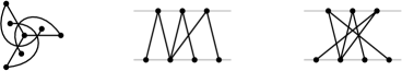
Fig. 1: The smallest tree $G$ that is not a caterpillar with a topological drawing with $\operatorname{max-cr}(G)=M(G)=9$ crossings (left), a $2$-layer drawing with $\operatorname{bcr}(G)=1$ crossings (middle) and a $2$-layer drawing with $\operatorname{max-\overline{cr}}(G)=M(G)-\operatorname{bcr}(G)=8$ crossings (right).

Particularly nice are separated convex drawings, i.e., separated drawings with vertices in convex position; see Fig. 1 for an example. Drawing bipartite graphs in the separated convex model is equivalent to the $2$-layer model where the vertices of the two color classes are required to be placed on two parallel lines. In this $2$-layer model, the crossing minimization of a bipartite graph $G$ has been studied under the name bipartite crossing number, denoted $\operatorname{bcr}(G)$.

Lemma 2.

For every bipartite graph $G$, the maximum number of crossings among all separated convex drawings of $G$ is exactly $M(G)-\operatorname{bcr}(G)$.

Proof.

Consider any separated convex drawing of any bipartite graph $G$. A pair of independent edges is crossing if and only if their endpoints alternate along the convex hull. So if $e_{1}=u_{1}v_{1}$ and $e_{2}=u_{2}v_{2}$ with $u_{1},u_{2}$ being above the separating line $\ell$ and $v_{1},v_{2}$ below, then $e_{1}$ and $e_{2}$ are crossing if in the circular order we see $u_{1}-u_{2}-v_{1}-v_{2}$, and non-crossing if we see $u_{1}-u_{2}-v_{2}-v_{1}$. In particular, reversing the order of all vertices below the separating line $\ell$ transforms crossings into non-crossings and vice versa. This shows that for a separated convex drawing with $k$ crossings, reversing results in exactly $M(G)-k$ crossings, which concludes the proof. ∎

Applying Lemma 2 to the chain of inequalities (2) shows that for every bipartite graph $G$ we have

$$M(G)/2\leq M(G)-\operatorname{bcr}(G)\leq\operatorname{max-cr^{\circ}}(G)\leq\operatorname{max-\overline{cr}}(G)\leq\operatorname{max-cr}(G)\leq M(G).$$ (3)

It remains open whether the new inequality $M(G)-\operatorname{bcr}(G)\leq\operatorname{max-cr^{\circ}}(G)$ in (3) is attained with equality for every bipartite graph $G$. For example, for a tree $G$ it is known, see e.g. [Woo71], that $\operatorname{max-cr}(G)=M(G)$, but it is not hard to see that $\operatorname{max-\overline{cr}}(G)=M(G)$ if and only if $G$ is a caterpillar. (Hence $\operatorname{max-\overline{cr}}(G)<\operatorname{max-cr}(G)$ holds for every tree which is not a caterpillar.) Moreover, it is equally easy to see that a tree $G$ has a crossing-free $2$-layer drawing if and only if $G$ is a caterpillar. Thus, for every tree $G$, we have that $M(G)-\operatorname{bcr}(G)=M(G)$ if and only if $\operatorname{max-\overline{cr}}(G)=M(G)$. We again refer to Fig. 1 for an illustration.

The expanded chain on inequalities (3), leads to two natural questions:

Problem 1.

Does every bipartite graph $G$ have a separated drawing with $\operatorname{max-\overline{cr}}(G)$ many crossings? Does every tree $G$ have a separated convex drawing with $\operatorname{max-\overline{cr}}(G)$ crossings, i.e., is $\operatorname{max-\overline{cr}}(G)=M(G)-\operatorname{bcr}(G)$?

Let us mention that Garey and Johnson [GJ83] have shown that bipartite crossing minimization is NP-hard. The problem remains NP-hard if the ordering of the vertices on one side is prescribed [EW94]. On trees, bipartite crossing minimization can be solved efficiently [SSSV01]. For the one-sided two-layer crossing minimization, Nagamochi [Nag05] gave an $1.47$-approximation algorithm, improving upon the well-known median heuristic, which yields a $3$-approximation [EW94]. The weighted case, which we define formally in Section 4, admits a 3-approximation algorithm [ÇEKS09].

3 Counterexamples for Conjecture 1

In this section we present counterexamples for the convexity conjecture. After some preliminary work we provide a counterexample $H(4)$ on $37$ vertices. To show that this graph is a counterexample, we need to analyze only two cases. (To show that $H(2)$ with $19$ vertices also is a counterexample would require more work. Instead, in Appendix A, we prove that a certain planar subgraph of $H(2)$ with only $12$ vertices and $16$ edges is already a counterexample.)

A set of vertices $X\subset V$ in a graph $G=(V,E)$ is a set of twins if all vertices of $X$ have the same neighborhood in $G$ (in particular $X$ is an independent set). A vertex split of vertex $v$ in $G$ consists in adding a new vertex $v^{\prime}$ to $G$ such that $v^{\prime}$ is a twin of $v$, that is, for any edge $vu$, there is an edge $v^{\prime}u$, and these are all the edges at $v^{\prime}$.

Lemma 3.

For any graph $G$ there is a convex drawing of $G$ maximizing the number of crossings among all convex drawings of $G$, such that each set of twins forms an interval of consecutive vertices along the convex hull of the drawing.

Proof.

Suppose $V_{1},\dots,V_{s}$ are the maximal sets of twins in $G$. Consider a convex drawing of $G$ maximizing the number of crossings. It clearly suffices to show that for any set $V_{i}$ we may move all the points of $V_{i}$ next to one of the points of $V_{i}$ without decreasing the number of crossings, since this procedure done iteratively $s$ times, once for each of the sets $V_{1},\dots,V_{s}$, results in a desired convex drawing of $G$.

We call a crossing $k$-rich if there are $k$ vertices of $V_{i}$ among the four vertices of the edges forming the crossing. Since $V_{i}$ is independent, $k$ is $0$, $1$ or $2$ for each crossing. If we move only vertices of $V_{i}$ then $0$-rich crossings remain in the drawing. If the vertices of $V_{i}$ appear in consecutive order along the convex hull of the drawing then the number of $2$-rich crossings is maximized due to the following argument. For any two vertices $u,v$ of $V_{i}$ and for any two neighbors $x,y$ of $V_{i}$, the $4$-cycle $uxvy$ is self-crossing which gives rise to a $2$-rich crossing. Since every $2$-rich crossing appears in a single $4$-cycle and every $4$-cycle can give rise to at most one crossing, the number of $2$-rich crossings is indeed maximized whenever the vertices of $V_{i}$ appear in consecutive order along the convex hull. It remains to show that there is a vertex $v$ in $V_{i}$ such that we can move the other vertices next to $v$ without decreasing the number of $1$-rich crossings. Each $1$-rich crossing involves exactly one vertex of $V_{i}$. The number of $1$-rich crossings involving a given vertex of $V_{i}$ is affected only by the position of that vertex and of the vertices of $V\setminus V_{i}$. Thus, if we choose $v$ as the vertex involved in the largest number of $1$-rich crossings and move all the other vertices of $V_{i}$ next to $v$, every vertex will be involved in at least as many $1$-rich crossings as it was before the vertices were moved. ∎

The construction of $H(k)$.

For the construction of our example graphs $H(k)$, we start with a 9-cycle on vertices $v_{0},\ldots,v_{8}$ with edges $v_{i},v_{i+1}$ where $i+1$ is to be taken modulo 9. Add a ‘central’ vertex $z$ adjacent to $v_{0},v_{3},v_{6}$. This graph on 10 vertices is the base graph $H$. The example graph $H(k)$ is obtained from $H$ by applying $k$ vertex splits to each of the nine cycle vertices $v_{i}$. The graph $H(k)$ thus consists of nine independent sets $V_{i}$ of size $k$ and the central vertex $z$. In total it has $9k+1$ vertices and $9k^{2}+3k$ edges. Figure 2 (left) shows a schematic drawing of $H(k)$, where each black edge represents a “bundle” of $k^{2}$ edges of $H(k)$ and each gray edge represents a set of $k$ edges. We will show that for $k\geq 4$ the drawing in Fig. 2 (right) has more crossings than any drawing with vertices in convex position.

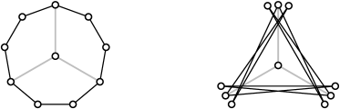
Fig. 2: Left: The graph $H(k)$. Each circle represents $k$ independent vertices, each black line segment represents a bundle of $k^{2}$ edges, each gray line segment represents $k$ edges. Right: A non-convex drawing of $H(k)$.

From Lemma 3 we know that, in convex drawings of $H(k)$ with many crossings, the twin pairs of vertices can be assumed to be next to each other. Drawings of $H(k)$ of this kind are essentially determined by the corresponding drawings of $H$, in which each set of twins is represented just by one representative; see Fig. 2. This justifies that later on we only look at convex drawings of $H$ with weighted crossings, and not of the full $H(k)$.

An independent set of edges of $H(k)$ is weak if the corresponding edges in the base graph $H$ are not independent; it is strong otherwise. The next lemma shows that our drawing of $H(k)$ realizes as many crossings on weak pairs of independent edges as possible. This allows us to focus on strong pairs in the subsequent analysis.

Lemma 4.

The drawing of $H(k)$ on the right side of Fig. 2 maximizes the number of crossings on weak pairs of independent edges.

Proof.

Each edge $v_{i},v_{i+1}$ of $H$ maps to a $K_{k,k}$ in $H(k)$. In the given drawing the $K_{k,k}$ is represented by a red edge. Since $V_{i}\cup V_{i+1}$ are in separated convex position the $K_{k,k}$ contributes $\binom{k}{2}^{2}$ crossing.

A pair of adjacent edges $v_{i-1},v_{i}$ and $v_{i},v_{i+1}$ in $H$ maps to a $K_{k,2k}$ in $H(k)$. We know that $\operatorname{max-\overline{cr}}(K_{k,2k})=\binom{k}{2}\binom{2k}{2}$ and this number of crossings is realized with separated convex position. In the drawing $V_{i}$ and $V_{i-1}\cup V_{i+1}$ are in separated convex position.

A pair of adjacent edges $v_{i},z$ and $v_{i},v_{i+1}$ in $H$ maps to a $K_{k,k+1}$ in $H(k)$. Now we have $\operatorname{max-\overline{cr}}(K_{k,k+1})=\binom{k}{2}\binom{k+1}{2}$, and this number of crossings is realized with separated convex position of the vertices. In the drawing $V_{i},V_{i+1}\cup\{z\}$ are in separated convex position. The case of adjacent edges $v_{i},z$ and $v_{i-1},v_{i}$ is identical. ∎

The remaining crossings of the drawing of $H(k)$ correspond to crossings of two independent edges of $H$. These are either two red edges or a red and a green edge of $H$. Red edges represent a bundle of $k^{2}$ edges of $H(k)$ and green edges a bundle of $k$ edges of $H(k)$. Hence a crossing of two red edges represents $k^{4}$ individual crossing pairs and a crossing of a red and a green edge represent $k^{3}$ individual crossing pairs. We devide by $k^{3}$ and speak about a crossing of two red edges as a crossing of weight $k$ and of a red green crossing as a crossing of weight 1. In the given drawing of $H(k)$ every pair of red edges is crossing but every red edge has a unique independent green edge which is not crossed. Hence, the weight of the independent not crossing pairs of edges of $H$ is 9. We summarize by saying that the given drawing has a weighted loss of 9.

The loss of convex drawings.

We now study the weighted loss of convex drawings of $H$. In a convex drawing every red edge splits the 7 non-incident cycle vertices into those on one side and those on the other side. The span of a red edge is the number of vertices on the smaller side. Hence, the span of an edge is one of 0, 1, 2, 3.

Let us consider the case where the 9-cycle is drawn with zero loss, i.e., each red edge has span 3 and contributes a crossing with 6 other red edges. The cyclic order of the cycle vertices is $v_{0},v_{2},v_{4},v_{6},v_{8},v_{1},v_{3},v_{5},v_{7}$. Any two neighbors of $z$ have the same distance in this cyclic order. Therefore, we may assume that $z$ is in the short interval spanned by $v_{0}$ and $v_{6}$. Every edge of the 9-cycle is disjoint from at least one of the two green edges $z,v_{0}$ and $z,v_{6}$ and the edge $v_{7},v_{8}$ is disjoint from both. This shows that the weighted loss of this drawing is at least 10.

A sequence of eight consecutive edges of span 3 forces the last edge to also have span 3. Hence, we have at least two red edges $e$ and $f$ of span at most 2. Each of these edges is disjoint from at least two independent red edges. Since the two edges may be disjoint they contribute a weighted loss of at least $3k$. For $k>4$ this exceeds the weighted loss of the drawing of Fig. 2.

4 Complexity

Very recently, Bald et al. [BJL16] showed, by reduction from MaxCut, that it is NP-hard to compute the maximum rectilinear crossing number $\operatorname{max-\overline{cr}}(G)$ of a given graph $G$. Their reduction also shows that it is hard to approximate the weighted case better than $\approx 0.878$ assuming the Unique Games Conjecture and better than $16/17$ assuming ${\cal P}\neq{\cal NP}$. In the convex case, one can “guess” the permutation; hence, this special case is in $\cal NP$. Bald et al. also stated that rectlinear crossing maximization is similar to rectilinear crossing minimization in the sense that the former “inherits” the membership in the class of the existential theory of the reals ($\exists\mathbb{R}$), and hence in PSPACE, from the latter. They also showed how to derandomize Verbitsky’s approximation algorithm [Ver08] for $\operatorname{max-\overline{cr}}$, turning the expected approximation ratio of $1/3$ into a deterministic one.

We now tighten the hardness results of Bald et al. by showing APX-hardness for the unweighted case. Recall that MaxCut is NP-hard to approximate beyond a factor of $16/17$ [Hås01]. Under the Unique Games Conjecture, MaxCut is hard to approximate even beyond a factor of $\approx\!0.878$ [KKMO07]—the approximation ratio of the famous semidefinite programming approach of Goemans and Williamson [GW95] for MaxCut. For a graph $G$, let $\operatorname{max-cut}(G)$ be the maximum number of edges crossing a cut, over all cuts of $G$.

Theorem 1.

Given a graph $G$, $\operatorname{max-\overline{cr}}(G)$ cannot be approximated better than MaxCut.

Proof.

As Bald et al., we reduce from MaxCut. In their reduction, they add a large-enough set $I$ of independent edges to the given graph $G$. They argue that $\operatorname{max-\overline{cr}}(G+I)$ is maximized if the edges in $I$ behave like a single edge with high weight that is crossed by as many edges of $G$ as possible. Indeed, suppose for a contradiction that, in a drawing with the maximum number of crossings, an edge $e\in I$ crosses fewer edges than another edge $e^{\prime}$ in $I$. Then $e$ can be drawn such that its endpoints are so close to the endpoints of $e^{\prime}$ that both edges cross the same edges—and each other. This would increase the number of crossings; a contradiction. W.l.o.g., we can make the “heavy edge” so long that its endpoints lie on the convex hull of the drawing. This means that the heavy edge induces a cut of $G$. The cut is maximum since the heavy edge can be made arbitrarily heavy.

Instead of adding a set $I$ of independent edges to $G$, we add a star $S_{t}$ with $t=\binom{m}{2}+1$ edges, where $m=|E(G)|$. Then, $\operatorname{max-\overline{cr}}(G)<t$. The advantage of the star is that all its edges are incident to the same vertex and, hence, cannot cross each other. Let $G^{\prime}=G+S_{t}$ be the resulting graph. Exactly as for the set $I$ above, we argue that all edges of $S_{t}$ must be crossed by the same number of edges of $G$, and must in fact form a cut of $G$. Hence, we get

$$t\cdot\operatorname{max-cut}(G)\leq\operatorname{max-\overline{cr}}(G^{\prime})\leq t\cdot\operatorname{max-cut}(G)+\operatorname{max-\overline{cr}}(G)<t\cdot(\operatorname{max-cut}(G)+1).$$

This yields $\operatorname{max-cut}(G)=\lfloor\operatorname{max-\overline{cr}}(G^{\prime})/t\rfloor$. Hence, any $\alpha$-approximation for maximum rectilinear crossing number yields an $\alpha$-approximation for MaxCut. ∎

With the same argument, we also obtain hardness of approximation for $\operatorname{max-cr^{\circ}}$, which was only shown NP-hard by Bald et al. [BJL16]. The reason is that in the convex setting, too, the “heavy obstacle” splits the vertex set into a “left” and a “right” side.

Corollary 1.

Given a graph $G$, $\operatorname{max-cr^{\circ}}(G)$ cannot be approximated better than MaxCut.

Next we consider the weighted topological case, which is formally is defined as follows. For a graph $G$ with positive edge weights $w\colon E\to\mathbb{Q}_{>0}$ and a drawing $D$ of $G$, let $\operatorname{max-wt-cr}(D)=\sum_{e\text{ crosses }e^{\prime}}w(e)\cdot w(e^{\prime})$ be the weighted maximum crossing number of $D$, and let $\operatorname{max-wt-cr}(G)$ be the maximum $\operatorname{max-wt-cr}(D)$ over all drawings $D$ of $G$ be the weighted maximum crossing number of $G$. Let MaxWtCrNmb be the problem of computing the weighted maximum crossing number of a given graph.

Compared to the rectilinear and the convex case above, the difficulty of the topological case is that an obstacle (such as the heavy star above) does not necessarily separate the vertices into “left” and a “right” groups any more. Instead, our new obstacle separates the vertices into an “inner” group and an “outer” group, which allows us to reduce from a cut-based problem.

Our new starting point is the NP-hard problem 3MaxCut [Yan78], which is the special case of MaxCut where the input graph is required to be 3-regular.

Theorem 2.

Given an edge-weighted graph $G$, computing $\operatorname{max-wt-cr}(G)$ is NP-complete.

Proof.

Clearly, topological crossing maximization is in $\cal NP$ since we can guess a rotation system for the given graph and, for each edge, the ordered subset of the other edges that cross it. In polynomial time, we can then check whether (a) the weights of the crossings sum up to the given threshold, and (b) the solution is feasible, simply by realizing the crossings via dummy vertices of degree 4 and testing for planarity of the so-modified graph.

To show NP-hardness, we reduce from 3MaxCut. Given an instance of 3MaxCut, that is, a 3-regular graph $G$, we construct an instance of topological crossing maximization, that is, a weighted graph $G^{\prime}$. Let $G^{\prime}$ be the disjoint union of $G$ with edges of weight 1 and a single triangle $T$ with edges of (large) weight $t$. Any edge of $G$ that connects a vertex in the interior of $T$ to a vertex in the exterior of $T$ can cross $T$ up to three times (that is, each edge of $T$ once). Any edge that connects two vertices in the interior (or two vertices in the exterior) of $T$ can cross $T$ at most twice. In any 3-regular graph $(V,E)$, it holds that $|E|=3/2\cdot|V|$. Due to the 3-regularity of $G$, we have that, for each vertex in $V$, at least two of its incident edges are in a maximum cut. Hence, $\operatorname{max-cut}(G)\geq 2/3\cdot m=n$, where $n$ and $m$ are the numbers of the vertices and edges of $G$. Let $C=(V_{1},V_{2})$ be any maximum cut of $G$. Since any vertex has at most one edge that does not cross $C$, the edges in $G[V_{1}]$ form a matching $M_{1}$ and the edges in $G[V_{2}]$ form a matching $M_{2}$.

Fig. 3: Given a 3-regular graph $G$, a drawing of $G^{\prime}=G+T$ with the maximum number of crossings yields a maximum cut of $G$ if the edges of the triangle $T$ have much larger weight than the edges of $G$. The edges (in the light blue region) that cross $T$ trice are in the cut.

Fig. 4: A crossing-maximal drawing of the complete tripartite graph $K_{k,k,k}$.

Consider a drawing of $G^{\prime}$ as in Fig. 4. For $i\in\{1,2\}$, partition the vertices in $V_{i}$ into a left subset $L_{i}$ and a right subset $R_{i}$ so that all edges in $M_{i}$ go from left to right. Each edge in the cut crosses all edges of $T$. Each edge in $M_{1}\cup M_{2}$ crosses exactly two edges of $T$. Clearly, $\operatorname{max-cr}(G)\leq\binom{m}{2}=\binom{3n/2}{2}<9/8\cdot n^{2}$. To ensure that one crossing of an edge of $T$ contributes more than this, we set $t=9/8\cdot n^{2}$. Since any edge of $G$ crosses triangle $T$ at least twice, we get the lower bound $\operatorname{max-wt-cr}(G^{\prime})\geq t(2m+\operatorname{max-cut}(G))$ and the upper bound $\operatorname{max-wt-cr}(G^{\prime})\leq 2mt+t\cdot\operatorname{max-cut}(G)+\operatorname{max-cr}(G)<t(2m+\operatorname{max-cut}(G)+1)$, which yields $\operatorname{max-cut}(G)=\lfloor\operatorname{max-wt-cr}(G^{\prime})/t\rfloor-2m$. ∎

In Appendix B we argue why it is unlikely that MaxWtCrNmb admits a PTAS.

We now set out to strengthen the result of Theorem 2; we want to show that even the unweighted maximum crossing number is hard to compute. Observe that in the above proof, the given graph $G$ from the 3MaxCut instance remained unweighted, but we required a heavily weighted additional triangle $T$. Our goal is now, essentially, to substitute $T$ with an unweighted structure that serves the same purpose. Unfortunately, due to the large number of crossings of this new structure, we cannot make any statement about non-approximability of the unweighted case. The naïve approach of simply adding multiple unweighted triangles does not easily work since already the entanglement of the triangles among each other is non-trivial to argue.

Theorem 3.

Given a graph $G$, $\operatorname{max-cr}(G)$ is NP-complete to compute.

Proof.

The membership in $\cal NP$ follows from Theorem 2. To argue hardness, given an instance $G$ of 3MaxCut, we construct an unweighted graph $G^{\prime}$—the instance for computing $\operatorname{max-cr}(G^{\prime})$—as the disjoint union of $G$ and a complete tripartite graph $K:=K_{k,k,k}$ with $k$ vertices per partition set, $k>\sqrt{9/8}\cdot n$. A result of Harborth [Har76] yields $\operatorname{max-cr}(K)=\binom{3k}{4}-3\binom{k}{4}-6k\binom{k}{3}\in\Theta(k^{4})$.

We first analyze a crossing-maximal drawing of $K$; see Fig. 4. Consider a straight-line drawing “on a regular hexagon $\mathcal{H}$”. Let $V_{1},V_{2},V_{3}$ be the partition sets of $K$ and label the edges of $\mathcal{H}$ cyclically $1,2,\ldots,6$. Place $V_{i}$, $1\leq i\leq 3$, along edge $2i$ of $\mathcal{H}$. We claim that $\operatorname{max-cr}(K)$ is achieved by this drawing. In fact, the arguments are analogous to the maximality of the naïve drawing for complete bipartite graphs on two layers: a 4-cycle can have at most one crossing. In the above drawing, every 4-cycle has a crossing. On the other hand, any crossing in any drawing of $K$ is contained in a 4-cycle.

Intuitively, when thinking about shrinking the sides $1,3,5$ in $\mathcal{H}$, we obtain a drawing akin to $T$ in the hardness proof for the weighted maximum crossing number. It remains to argue that there is an optimal drawing of full $G^{\prime}$ where $K$ is drawn as described. Consider a drawing realizing $\operatorname{max-cr}(G^{\prime})$ and note that any triangle in $K$ is formed by a vertex triple, with a vertex from each partition set. Pick a triple $\tau=(v_{1},v_{2},v_{3})\in V_{1}\times V_{2}\times V_{3}$ that induces a triangle $T_{\tau}$ with maximum number of crossings with $G$ among all such triangles. Now, redraw $K$ along $T_{\tau}$ according to the above drawing scheme such that, for $i=1,2,3$, it holds that (a) all vertices of $V_{i}$ are in a small neighborhood of $v_{i}$ and (b) any edge $(w_{i},w_{j})\in V_{i}\times V_{j}$ for some $j\neq i$ crosses exactly the same edges of $G$ as the edge $(v_{i},v_{j})$. Our new drawing retains the same crossings within $G^{\prime}$, achieves the maximum number of crossings within $K$, and does not decrease the number of crossings between $K$ and $G$; hence it is optimal. In this drawing, $K$ plays the role of the heavy triangle $T$ in the hardness proof of the weighted case, again yielding NP-hardness. ∎

5 Conclusions and Open Problems

We have considered the crossing maximization problem in the topological, rectilinear, and convex settings. In particular, we disproved a conjecture of Alpert et al. [AFH09] that the maximum crossing number in the latter two settings always coincide. On the other hand, we propose a new setting, the “separated drawing” setting, and ask whether for every bipartite graph the maximum rectilinear, maximum convex, maximum separated, and maximum separated convex crossing numbers coincide.

Concerning complexity, we have shown that the maximum rectilinear crossing number is APX-hard and the maximum topological crossing number is NP-hard. A natural question then is whether the maximum topological crossing number is also APX-hard. We have shown this to be true in the weighted topological case. It also remains open whether rectilinear crossing maximization is in $\cal NP$, which would have followed if the rectilinear and convex setting were equivalent as conjectured by Alpert et al.. A reviewer of an earlier version of this paper was wondering about the complexity of maximum crossing number for planar graphs. For planar graphs, MaxCut is tractable and our hardness arguments no longer apply, leaving open the question of the complexity of computing the maximum crossing number for this graph class.

Other intriguing crossing maximization problems remain open: apart from the two classic problems that we mentioned above—Conway’s Thrackle Conjecture and Ringeisen’s Subgraph Problem—we are interested in the separation of the rectilinear and the separated convex setting for bipartite graphs.

Acknowledgments.

Work on this problem started at the 2016 Bertinoro Workshop of Graph Drawing. We thank the organizers and other participants for discussions, in particular Michael Kaufmann. We also thank Marcus Schaefer, Gábor Tardos, and Manfred Scheucher.

Appendix

Appendix A Counterexamples with 12 Vertices

Here we provide three similar graphs with $12$ vertices and $16$ edges violating the convexity conjecture (Conjecture 1). Note that each graph is planar and has maximum degree $4$ or $5$. This shows that the convexity conjecture is false also for some natural graph classes such as planar graphs or graphs with maximum degree at most four. Our proof is based on a relatively long case-analysis. Manfred Scheucher independently verified by a computer search that these three graphs indeed violate the convexity conjecture. Moreover, his unsuccessful attempts to find a smaller counterexample with the use of computer search support our feeling that the convexity conjecture might hold for all graphs on at most $11$ vertices.

Let $H$ be the graph with $10$ vertices and $12$ edges from the previous subsections. We distinguish three types of vertices: $A$-vertices, $B$-vertices, and $C$-vertices. The central vertex is the only $A$-vertex. The three vertices $v_{0},v_{3},v_{6}$ of $H$ connected to the central vertex are the $B$-vertices and the six vertices in $H$ of degree two are $C$-vertices. The three edges adjacent to the $A$-vertex are called $\alpha$-edges, the six edges connecting a $B$-vertex with a $C$-vertex are called $\beta$-edges and the remaining three edges connecting independent pairs of $C$-vertices are called $\gamma$-edges. The nine $B$- and $C$-vertices are cycle vertices, and the nine $\beta$- and $\gamma$-edges forming a $9$-cycle are called cycle edges.

Fig. 5: The graph $H$ (left), the three possible graphs $H_{16}$ (middle), and the weighted graph $W_{14}$ (right).

We choose $H_{16}$ as a graph obtained from $H$ by selecting a pair of non-adjacent $C$-vertices and replacing each of them by a pair of independent vertices. Since the $C$-vertices have degree two in $H$, four edges of $H$ are replaced by a copy of $K_{1,2}$, thus the graph $H_{16}$ has $12$ vertices and $16$ edges. Up to isomorphism, $H_{16}$ is one of the three planar graphs depicted in the middle of Fig. 5. It corresponds to the weighted graph $W_{16}$ which is the graph $H$ with edge weights, where two of the $\beta$-edges have weight two, two of the $\gamma$-edges have weight two, and the remaining eight edges have weight one. Further, let $W_{14}$ be the same weighted graph with the exception that all the $\beta$-edges have weight one, see the right of Fig. 5. Thus, only two $\gamma$-edges have weight two, otherwise the edges in $W_{14}$ have weight one. The graph $W_{14}$ is, up to isomorphism, uniquely determined regardless of the graph $H_{16}$.

We now give two lemmas used in the proof that $H_{16}$ is a counterexample for the convexity conjecture.

Lemma 5.

In any drawing of $H$, any cycle edge avoids another edge.

Proof.

Let $e$ be a cycle edge. Then there is a $5$-cycle $Z$ consisting of edges non-adjacent to $e$. (The cycle $Z$ contains two $\alpha$-edges, two $\beta$-edges and one $\gamma$-edge.) There must be two consecutive vertices of $Z$ lying on the same side of the edge $e$ in the considered drawing. The edge connecting these two vertices is avoided by $e$. ∎

Lemma 6.

In any convex drawing of $H$, any cycle edge of span $s\in\{0,1,2\}$ avoids at least $6-2s$ cycle edges.

Proof.

Let $e$ be a cycle edge of span $s$. We first give an upper bound on the number of edges incident to $e$. The edge $e$ is incident to exactly one cycle edge at each of its two vertices. Since every cycle edge intersecting $e$ is incident to one of the $s$ cycle vertices of the “span interval” of $e$, at most $2s$ cycle edges intersect $e$. Altogether, at most $2+2s$ cycle edges different from $e$ have a point in common with $e$. Since there are eight cycle edges different from $e$, the edge $e$ avoids at least $8-(2+2s)=6-2s$ cycle edges. ∎

We now fix a convex drawing $D$ of $H_{16}$ maximizing the number of crossings and with twins placed next to each other. It gives a convex drawing of the weighted graph $W_{14}$ in the way described above. Since there is a non-convex drawing of $H_{16}$ with loss $13$, we need to show that the loss of the drawing $D$ of $H_{16}$ is at least $14$. From Lemma 5, applied on the drawing $D$, the loss of $H_{16}$ and the weighted loss of the corresponding drawing of $W_{14}$ differ by at least two. Thus, it suffices to show that the weighted loss of the drawing of $W_{14}$ given by the drawing $D$ is at least $12$. Before proving it, we fix some notation.

The nine $B$- and $C$-vertices of $W_{14}$ are denoted by $1,2,\dots,9$ in the counterclockwise order in which they appear in the drawing $D$. Without loss of generality we may assume that the $B$-vertices are $1$, $j$, $k$, where $1<j<k\leq 9$ and the vertex $A$ lies in the counterclockwise interval $(k,1)$. In other words, the three vertices $k,A,1$ appear in this counterclockwise order along the convex hull of the vertex set of $D$.

In the following, if a $\beta$-edge avoids a $\gamma$-edge in $D$, we say that there is a $\beta\gamma$-avoidance. Similarly we define $\beta\beta$-avoidances as avoidances of pairs of the $\beta$-edges, and $\gamma\gamma$-avoidances as avoidances of pairs of the $\gamma$-edges. Finally, $\alpha*$-avoidances are avoidances of pairs of edges that contain an $\alpha$-edge.

Lemma 7.

There are at least $2(k-2)$ $\alpha*$-avoidances.

Proof.

Let $X$ be the set of the $k-2$ vertices $2,3,\dots,k-1$. If a cycle edge connects two vertices of $X$ then it avoids the $\alpha$-edges $A1$ and $Ak$. If a cycle edge is incident to one of the vertices of $X$ then it avoids one of the $\alpha$-edges $A1$ and $Ak$. Thus, for each cycle edge $e$, the number of $\alpha$-edges avoided by $e$ is at least as big as the number of incidences of $e$ with $X$. Since the total number of incidences of the vertices in $X$ with the cycle edges is exactly $2|X|=2(k-2)$, the number of $\alpha*$-avoidances is at least $2(k-2)$. ∎

We now distinguish six cases.

Case 1: $k=3$ and there is no $\gamma\gamma$-avoidance.

In this case the $\beta$-vertices are $1$, $2$, $3$ and the three $\gamma$-edges are $47$, $58$, and $69$. Each of them has span $2$ and therefore, by Lemma 6, it avoids at least two of the $\beta$-edges. Since the total weight of the $\gamma$-edges is $5$, the $\beta\gamma$-avoidances have total weight at least $10$. Since there are at least two $\alpha*$-avoidances by Lemma 7, we get that the weighted loss of the drawing of $W_{14}$ (i.e., the total weighted number of avoidances) is at least $12$ in Case 1.

Case 2: $k=3$ and there is a $\gamma\gamma$-avoidance.

The $\beta$-edge $\beta_{4}$ containing the vertex $4$ has the five $C$-vertices $5$, $6$, $7$, $8$, $9$ on the same side and therefore avoids two $\gamma$-edges. Since any two $\gamma$-edges have total weight three or four, it follows that $\beta_{4}$ appears in $\beta\gamma$-avoidances of total weight at least three. By symmetry, $\beta_{9}$ also appears in $\beta\gamma$-avoidances of total weight at least three.

The edge $\beta_{5}$ has the four $C$-vertices $6$, $7$, $8$, $9$ on the same side and therefore avoids at least one $\gamma$-edge. By symmetry, $\beta_{8}$ also avoids at least one $\gamma$-edge.

Summarizing, the edges $\beta_{5},\beta_{6},\beta_{8},\beta_{9}$ appear in $\beta\gamma$-avoidances of total weight at least $3+1+1+3=8$. Additionally, there are two $\alpha*$-avoidances and there is a $\gamma\gamma$-avoidance which is necessarily of weight two or four. It follows that the avoidances have total weight at least $8+2+2=12$.

Case 3: $k=4$ and there is no $\gamma\gamma$-avoidance.

Without loss of generality, we assume that the $B$-vertices are $1,3,4$. Then the $\gamma$-edges are $27$, $58$, $69$. The edge $58$ avoids the $\beta$-edges $\beta_{2}$ and $\beta_{9}$. Similarly, the edge $69$ avoids the $\beta$-edges $\beta_{2}$ and $\beta_{5}$. Since the edges $58$ and $69$ have total weight three or four, they appear in $\beta\gamma$-avoidances of total weight at least $3\cdot 2=6$.

The edge $\beta_{2}$ avoids either the two $\beta$-edges incident to the $C$-vertex $1$ or the two $\beta$-edges incident to the $C$-vertex $4$. Thus, there are at least two $\beta\beta$-avoidances. Also, there are at least four $\alpha*$-avoidances by Lemma 7. Altogether, the avoidances have total weight at least $6+2+4=12$.

Case 4: $k=4$ and there is a $\gamma\gamma$-avoidance.

As in Case 3, we assume that the $B$-vertices are $1,3,4$. The edge $\beta_{2}$ avoids two of the three $\gamma$-edges, which gives two $\beta\gamma$-avoidances of total weight three or four. The edge $\beta_{2}$ also avoids at least one $\beta$-edge connecting one of the vertices $1$ and $4$ with one of the vertices in the interval $[5,9]$.

Since there is a $\gamma\gamma$-avoidance, the interval $[5,9]$ contains the vertices of a $\gamma$-edge $\gamma_{0}$ of span at most $1$. The edge $\gamma_{0}$ avoids at least one $\gamma$-edge and at least two $\beta$-edges different from $\beta_{2}$ (for example, if $\gamma_{0}$ connects vertices $6$ and $8$, it avoids the $\beta$-edges $\beta_{5}$ and $\beta_{9}$). The $\gamma\gamma$-avoidance has weight two or four, and the two $\beta\gamma$-avoidances have total weight at least two.

Summarizing, avoidances involving no $\alpha$-edge have total weight at least $3+1+2+2=8$. Since there are at least four $\alpha*$-avoidances by Lemma 7, all avoidances have total weight at least $8+4=12$.

Case 5: $k=5$.

The two $\beta$-edges with both vertices in the interval $[1,5]$ have span at most $2$, and therefore appear in at least four avoidances among cycle edges. There are at least six $\alpha*$-avoidances by Lemma 7. It follows that there are at least ten avoidances.

Since each of the two $\gamma$-edges of weight two avoids another edge, there are at least two avoidances of weight two or an avoidance of weight four. We conclude that all the avoidances have total weight at least $10+2=12$.

Case 6: $k\geq 6$.

Suppose first that all nine cycle edges have span three. Then the cycle edges form the cycle $162738495$, The $B$-vertices are $1$, $4$, $7$, the $\gamma$-edge $26$ avoids the two $\alpha$-edges $A1$ and $A7$, and each of the other eight cycle edges avoids exactly one of the $\alpha$-edges $A1$, $A4$, $A7$. Thus, there are ten $\alpha*$-avoidances. Since each of the two $\gamma$-edges of weight two appears in at least two avoidances, the total weight of avoidances is at least $10+2=12$.

Suppose now that there is a cycle edge with span smaller than three. Then this edge avoids at least two cycle edges. Additionally there are at least eight $\alpha*$-avoidances. Altogether there are at least $2+8=10$ avoidances. Since each of the two $\gamma$-edges of weight two appears in some avoidance, all the avoidances have total weight at least $10+2=12$.

Appendix B It is Unlikely that MaxWtCrNmb Admits a PTAS

Due to the additive term $2m$ in the lower and upper bound for $\operatorname{max-wt-cr}(G)$ (see the sequence of inequalities at the end of the proof of Theorem 2), the existence of a PTAS for MaxWtCrNmb does not directly imply a PTAS for 3MaxCut. A PTAS for MaxWtCrNmb would, however, give us a very good estimation of the quantity $q=2m+\operatorname{max-cut}(G)$. Since $G$ is 3-regular, we know that $2m/3\leq\operatorname{max-cut}(G)\leq m$. Hence, assuming a $(1-\varepsilon)$-approximation of $\operatorname{max-cut}(G)$, the ratio between the smallest and the largest possible value of $q$ is $(8m/3-\varepsilon)/(3m)=8/9-\varepsilon^{\prime}=0.\overline{8}-\varepsilon^{\prime}$. This would be the approximation ratio of an algorithm for 3MaxCut based on a hypothetical PTAS for MaxWtCrNmb. 3MaxCut is APX-hard; the best known inapproximability ratio is 0.997 [BK99], which is too large to yield a contradiction to the existence of a PTAS for MaxWtCrNmb. However, to the best of our knowledge, the best approximation algorithm for 3MaxCut is the semidefinite program of Goemans and Williamson [GW95] for general MaxCut. Its approximation ratio is $\approx 0.878$, and any improvement beyond this factor, even for the special case of 3-regular graphs, would be rather unexpected.

References

- [AFH09] Matthew Alpert, Elie Feder, and Heiko Harborth. The maximum of the maximum rectilinear crossing numbers of -regular graphs of order . Electron. J. Combin., 16(1), 2009. URL: http://www.combinatorics.org/ojs/index.php/eljc/article/view/v16i1r54/0.
- [Bal85] Richard Baltzer. Eine Erinnerung an Möbius und seinen Freund Weiske. Berichte über die Verhandlungen der Königlich Sächsischen Gesellschaft der Wissenschaften zu Leipzig. Mathematisch-Physische Classe, 37:1–6, 1885.
- [BJL16] Samuel Bald, Matthew Johnson, and Ou Liu. Approximating the maximum rectilinear crossing number. In T. N. Dinh and M. T. Thai, editors, Proc. 22nd Int. Comput. Combin. Conf. (COCOON’16), volume 9797 of LNCS, pages 455–467. Springer, 2016. doi:10.1007/978-3-319-42634-1_37.
- [BK99] Piotr Berman and Marek Karpinski. On some tighter inapproximability results. In J. Wiedermann, P. van Emde Boas, and M. Nielsen, editors, Proc. 26th Int. Colloq. Autom. Lang. Program. (ICALP’99), volume 1644 of LNCS, pages 200–209. Springer, 1999. doi:10.1007/3-540-48523-6_17.
- [ÇEKS09] Olca A. Çakiroglu, Cesim Erten, Ömer Karatas, and Melih Sözdinler. Crossing minimization in weighted bipartite graphs. J. Discrete Algorithms, 7(4):439–452, 2009. doi:10.1016/j.jda.2008.08.003.
- [EW94] Peter Eades and Nicholas C. Wormald. Edge crossings in drawings of bipartite graphs. Algorithmica, 11:379–403, 1994. doi:10.1007/BF01187020.
- [FK77] W.H. Furry and D.J. Kleitman. Maximal rectilinear crossing of cycles. Studies Appl. Math., 56(2):159–167, 1977. doi:10.1002/sapm1977562159.
- [GJ83] Michael R. Garey and David S. Johnson. Crossing number is NP-complete. SIAM J. Alg. Disc. Methods, 4:312–316, 1983. doi:10.1137/0604033.
- [Grü72] Branko Grünbaum. Arrangements and spreads. CBMS Regional Conf. Series in Math., 10:27, 1972. doi:10.1090/cbms/010.
- [GW95] Michel X. Goemans and David P. Williamson. Improved approximation algorithms for maximum cut and satisfiability problems using semidefinite programming. J. ACM, 42(6):1115–1145, 1995.
- [Har76] Heiko Harborth. Parity of numbers of crossings for complete -partite graphs. Mathematica Slovaca, 26(2):77–95, 1976. URL: https://eudml.org/doc/33976.
- [Hås01] Johan Håstad. Some optimal inapproximability results. J. ACM, 48(4):798–859, 2001. doi:10.1145/502090.502098.
- [KKMO07] Subhash Khot, Guy Kindler, Elchanan Mossel, and Ryan O’Donnell. Optimal inapproximability results for MAX-CUT and other 2-variable CSPs? SIAM J. Comput., 37(1):319–357, 2007. doi:10.1137/S0097539705447372.
- [KPR+08] Mihyun Kang, Oleg Pikhurko, Alexander Ravsky, Mathias Schacht, and Oleg Verbitsky. Obfuscated drawings of planar graphs. ArXiv, 2008. URL: arxiv.org/abs/0803.0858v3.
- [LPS97] László Lovász, János Pach, and Mario Szegedy. On Conway’s thrackle conjecture. Discrete Comput. Geom., 18(4):369–376, 1997. doi:10.1007/PL00009322.
- [Nag05] Hiroshi Nagamochi. An improved bound on the one-sided minimum crossing number in two-layered drawings. Discrete Comput. Geom., 33(4):569–591, 2005. doi:10.1007/s00454-005-1168-0.
- [PRS91] Barry L. Piazza, Richard D. Ringeisen, and Sam K. Stueckle. Properties of nonminimum crossings for some classes of graphs. In Yousef Alavi et al., editor, Proc. 6th Quadrennial Int. 1988 Kalamazoo Conf. Graph Theory Combin. Appl., volume 2, pages 975–989. Wiley, New York, 1991. URL: https://www.zentralblatt-math.org/ioport/en/?id=2845087&type=pdf.
- [Rin64] Gerhard Ringel. Extremal problems in the theory of graphs. In Proc. Theory of Graphs and its Applications (Smolenice 1963), pages 85–90, 1964.
- [RSP91] Richard D. Ringeisen, Sam K. Stueckle, and Barry L. Piazza. Subgraphs and bounds on maximum crossings. Bull. Inst. Combin. Appl, 2:9–27, 1991.
- [Sch14] Marcus Schaefer. The graph crossing number and its variants: A survey. Electron. J. Combin., Dynamic Surveys(#DS21):100 pages, 2014. URL: http://www.combinatorics.org/ojs/index.php/eljc/article/view/DS21.
- [SSSV01] Farhad Shahrokhi, Ondrej Sýkora, László A. Székely, and Imrich Vrt’o. On bipartite drawings and the linear arrangement problem. SIAM J. Comput., 30:1773–1789, 2001. doi:10.1137/S0097539797331671.
- [Sta93] Hans Staudacher. Lehrbuch der Kombinatorik: Ausführliche Darstellung der Lehre von den kombinatorischen Operationen (Permutieren, Kombinieren, Variieren). J. Maier, Stuttgart, 1893. URL: https://archive.org/details/lehrbuchderkomb00staugoog.
- [Ste23] Ernst Steinitz. Über die Maximalzahl der Doppelpunkte bei ebenen Polygonen von gerader Seitenzahl. Mathematische Zeitschrift, 17(1):116–129, 1923. URL: https://eudml.org/doc/167730.
- [Ver08] Oleg Verbitsky. On the obfuscation complexity of planar graphs. Theoret. Comput. Sci., 396(1):294–300, 2008. doi:10.1016/j.tcs.2008.02.032.
- [Woo71] Douglas R. Woodall. Thrackles and deadlock. In D. Welsh, editor, Proc. Combinatorial Mathematics and its Applications, pages 335–347. Academic Press, 1971.
- [Yan78] Mihalis Yannakakis. Node- and edge-deletion NP-complete problems. In Proc. 10th Annu. ACM Symp. Theory Comput. (STOC’78), pages 253–264, 1978. doi:10.1145/800133.804355.