Dynamical patterns in active nematics on a sphere

Abstract

Using agent-based simulations of self-propelled particles subject to short-range repulsion and nematic alignment we explore the dynamical phases of a dense active material confined to the surface of a sphere. We map the dynamical phase diagram as a function of curvature, alignment strength and activity and reproduce phases seen in recent experiments on active microtubules moving on the surfaces of vesicles. At low driving, we recover the equilibrium nematic ground state with four $+1/2$ defects. As the driving is increased, geodesic forces drive the transition to a band of polar matter wrapping around an equator, with large bald spots corresponding to two $+1$ defects at the poles. Finally, bands fold onto themselves, followed by the system moving into a turbulent state marked by active proliferation of pairs of topological defects. We highlight the role of nematic persistence length and time for pattern formation in these confined systems with finite curvature.

I Introduction

Active matter consists of self-driven agents that individually dissipate energy and organise in collective self-sustained motion. Active systems are maintained out of equilibrium by a drive that acts independently on each agent, breaking time reversal symmetry locally, rather than globally as in more familiar condensed matter systems driven out of equilibrium by external fields or boundary forces. Realisations span many scales, both in the living and non-living world, from bird flocks to bacterial suspensions, epithelial cell layers and synthetic microswimmers Marchetti et al. (2013); Ramaswamy (2010).

Active particles are often elongated and form active liquid crystal phases, with either polar or nematic symmetry, and emergent patterns controlled by the interplay of orientational order and active flows. Novel effects predicted and observed in simulations and experiments include long-range order in two dimensions Vicsek et al. (1995), spontaneous laminar flow Voituriez et al. (2005), giant number fluctuations Simha and Ramaswamy (2002); Narayan et al. (2007); Chaté et al. (2006), novel rheology Hatwalne et al. (2004); Marchetti (2012), and active turbulence accompanied by the proliferation of topological defects that drive the self-sustained dynamics Sanchez et al. (2012). Very recently, topological defects have also been shown to affect cell death and extrusion in nematically ordered epithelia Saw et al. (2017) and neural progenitor cell cultures Kawaguchi et al. (2017). Much of this rich behaviour is captured well by active hydrodynamics.

Even more surprises arise when active systems are confined by bounding surfaces or to geometries that require defects in the orientational order. When confined to a box, active particles accumulate at the boundary, with the strongest accumulation at corners, demonstrating the dramatic effects of wall curvature Yang et al. (2014); Fily et al. (2016). When constrained to move on curved surfaces, as realised for instance when cells migrate in the gut epithelium Sato et al. (2009) or on the surface of the growing cornea Collinson et al. (2002), the interplay of activity and curvature can drive novel dynamical structures. Keber et al.  Keber et al. (2014) have studied this interplay under controlled conditions in active vesicles obtained by confining an active nematic suspension of kinesin-microtubule bundles to the surface of a lipid vesicle. Topological defects are unavoidable when a nematic liquid crystal is confined to the surface of a sphere, where the net topological charge must be $2$. In equilibrium the lowest energy configuration consists of four $+1/2$ disclinations arranged at the corner of a tetrahedron inscribed in the sphere Nelson (2002); Shin et al. (2008). In the active vesicles of Ref. Keber et al. (2014), this four-defect configuration oscillates at a well defined rate controlled by the concentration of ATP between the tetrahedral configuration and a planar one, with the four defects on an equator. A minimal model of $+1/2$ active defects as self-propelled particles Giomi et al. (2013), subsequent hydrodynamic descriptions Khoromskaia and Alexander (2016) and a particle-based extensile nematic simulation Alaimo et al. (2017) reproduce the oscillatory behaviour, but are inadequate to describe the rich succession of dynamical states observed when decreasing the size of the vesicles, including defect-driven protrusions, and two $+1$ aster defects at the poles with spontaneously folding nematic bands.

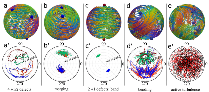
Figure 1: Active nematic patterns formed by agents self-propelled at speed $v_{0}$ on a sphere of radius $R$. Individual agents randomly reverse their direction of self propulsion at rate $\tau_{\text{flip}}^{-1}$ and align nematically with neighbours at rate $J$. Activity (quantified by $v_{0}$) increases from left to right (see also supplementary movies M1-M5). Top row: Nematic patterns and defect positions. Individual agents are represented by bars, coloured by the x-component of their director. Defects are represented by dots, coloured by charge (dark blue: $+1/2$, tan: $-1/2$, red: $+1$). Polarisation sorting and the formation of lanes traveling in opposite directions is evident in (d) and (e). Bottom row: Stereographic projections of defect trajectories in the corresponding states (see also Fig. S3 for the corresponding tracks). Here $+1/2$ / $-\!1/2$ defects are represented by black/red dots, $+1$ defects are green dots, and where possible, we have tracked defect trajectories in different colours. All images are for $\tau_{\mathrm{flip}}=100$ and $R=30$, except for (e) where $R=50$. (a, a’) Four $+1/2$ defects for $v_{0}=0.4$ and $J=1$; (b, b’) merging defect state for $v_{0}=1$, $J=5$ (b) and $v_{0}=1.2$ and $J=2$ (b’); (c, c’) band state for $v_{0}=1$, $J=0.1$ (c) and $v_{0}=1.2$ and $J=0.1$ (c’); (d, d’) bending bands for $v_{0}=2$, $J=0.1$ (d) and $v_{0}=2.5$ and $J=0.1$ (d’); (e, e’) active turbulence for $v_{0}=4$ , $J=1$ (e) and $v_{0}=5$ and $J=5$ (e’).

In this paper, we examine the rich dynamics of active nematics on a sphere by considering a model of soft self-propelled active agents with nematic alignment. The model reproduces a number of the curvature and activity induced dynamical structures observed in the experiments of Ref. Keber et al. (2014), including the oscillating state of four $+1/2$ disclinations, an equatorial nematic band, a state where the band folds on itself, and eventually the transition to turbulence with proliferation on unbound defect pairs. This rich succession of states obtained with increasing activity is shown in Fig. 1.

Circulating band states have also been reported by two of us in a simulation of soft self-propelled agents on a sphere, but with polar alignment Sknepnek and Henkes (2015). Recent work by one of us has additionally demonstrated that band formation on a sphere is a universal feature of the Toner-Tu equations for polar flocks  Shankar et al. (2017). It was also recently shown that on ellipsoids, the band localises to the low-curvature region Ehrig et al. (2016). Here we show that active nematics also exhibit band states arising from the interplay of active motion and curvature. Our work shows that the formation of the band state is a generic property of active systems, independent of their symmetry and that it arises from the intrinsic tendency of active particles to move along geodesics on curved surfaces. The identification of this key mechanism for driving pattern formation on curved topologies is an important result of our work.

A second, more subtle, finding concerns the emergence of hydrodynamics from agent-based models. Derivations of hydrodynamic equations from microscopic dynamics can be carried out at low density Marchetti et al. (2013), but become challenging in the dense limit Gao et al. (2015). In particular, although our system behaves like a nematic fluid at long times and large length scales, it also exhibits a substantial amount of short range polar order and local flocking at intermediate time scales, suggesting that a suitable continuum model may require inclusion of a polarisation field in conjunction to a nematic order parameter. A similar result was reported for a related model in the plane Shi and Ma (2013), hence is not the result of curvature. This behaviour is also reminiscent of that of collections of self-propelled rods Bertin et al. (2015) - polar active agents that exhibit nematic order at large scales. This local polar order becomes important in confined geometries like a sphere when the persistence length of the motion becomes comparable to the sphere radius and drives polarity sorting and leads to the folding band regime shown in Fig. 8. In the experiments of Ref. Keber et al. (2014) similar structures occur when the length of the microtubule bundles is comparable to the size of the vesicle.

The paper is organised as follows. In Sec. II we introduce the model of soft active agents moving on the surface of a 2-sphere. In Sec. III, we outline methods used to analyse behaviour of the system, followed by a detailed characterisation of the five distinct dynamical patterns that we have observed presented in Sec. IV. Finally, we conclude in Sec. V. In Appendix A we introduce the algorithms used for identifying and tracking defects.

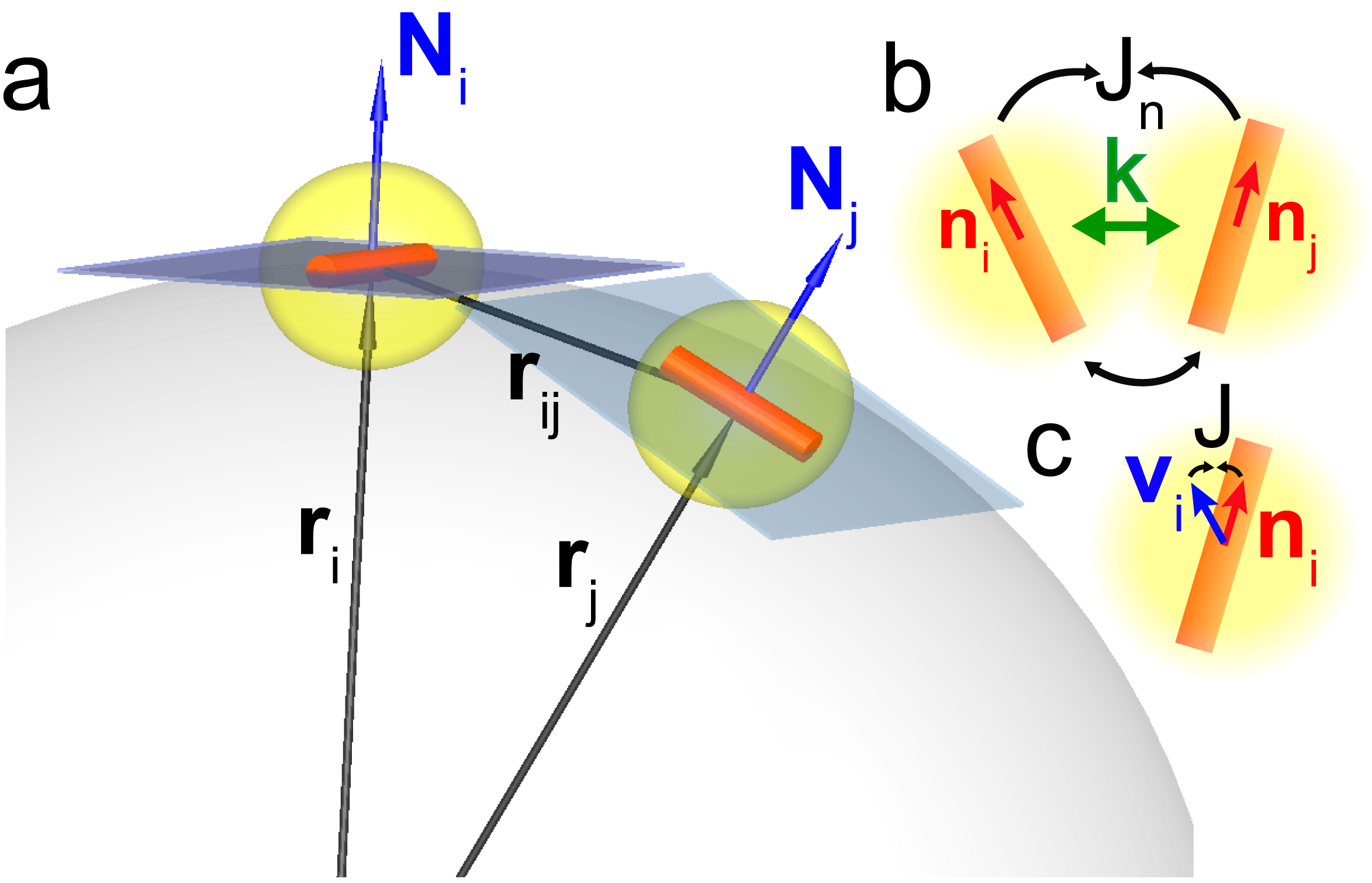
Figure 2: (Colour online) (a) Self-propelled agents are constrained to the surface of a sphere of radius $R$. Agents have an internal degree of freedom, the director $\mathbf{n}_{i}$ (red/dark cylinders). The position of each agent is given by $\mathbf{r}_{i}$, measured from the centre of the sphere. Distances between agents, $r_{ij}=\left|\mathbf{r}_{i}-\mathbf{r}_{j}\right|$, are calculated as the Euclidean distance in $\mathbb{R}^{3}$ space. (b) Agents are subject to a soft-core repulsion and experience torque which nematically aligns them to their immediate neighbours. (c) Additionally, each agent has a preference to align its director to the direction of its motion.

II Model: Soft active agents on a sphere

Active particles move through a medium that mediates long-range hydrodynamic interactions. Here we consider the dry limit, where the damping from the medium dominates over hydrodynamic interactions and the fluid only provides single-particle friction. Our system consists of $N$ self-propelled soft spherical agents of radius $\sigma$ confined to move on the surface of a 2-sphere of radius $R$ (Fig. 2 ). Each agent is characterised by its position $\mathbf{r}_{i}$ and a unit vector $\mathbf{n}_{i}$ or director denoting the direction of self-propulsion. Although confinement to the surface of a sphere implies that agent positions are parametrised by just two coordinates, e.g. azimuthal and polar angles, in numerical simulations it is more convenient to work in three-dimensional Euclidean space and explicitly impose the sphere constraint at each time step. This is accomplished through projection operators. The coupled equations for translational and rotational motion are then given by

$$\dot{\mathbf{r}}_{i} = \mathbf{P}^{T}_{i}\big{[}v_{0}\kappa_{i}(t)\mathbf{n}_{i}+\mu\sum\nolimits_{j}\mathbf{F}_{ij}\big{]}\;,$$ (1a)

$$\dot{\mathbf{n}}_{i} = \text{P}^{N}_{i}\big{[}-2J_{n}\sum\nolimits_{j}(\mathbf{n}_{i}\cdot\mathbf{n}_{j})(\mathbf{n}_{i}\times\mathbf{n}_{j})$$ (1b)

$$- 2J_{v}(\mathbf{v}_{i}\cdot\mathbf{n}_{i})(\mathbf{v}_{i}\times\mathbf{n}_{i})\big{]}(\hat{\mathbf{N}}_{i}\times\mathbf{n}_{i})\;,$$

where $\mathbf{P}^{T}_{i}[\mathbf{a}]=\mathbf{a}-(\hat{\mathbf{N}}_{i}\cdot\mathbf{a})\hat{\mathbf{N}}_{i}$ and $\text{P}^{N}_{i}[\mathbf{a}]=(\mathbf{a}\cdot\hat{\mathbf{N}}_{i})$ project any three-dimensional vector $\mathbf{a}$ onto the tangent plane and the surface normal to the sphere, respectively, with the local surface normal given by $\mathbf{\hat{N}}_{i}=\mathbf{r}_{i}/r_{i}$ Sknepnek and Henkes (2015).

The first term on the right hand side of Eq. (1a) describes self-propulsion at speed $v_{0}$. The nematic symmetry is implemented by reversing the direction of self propulsion at time intervals drawn from a Poisson distribution of mean $1/\tau_{\text{flip}}$ through a zero average bimodal noise $\kappa_{i}(t)=\pm 1$ Chaté et al. (2006). The second term in Eq. (1a) describes soft pairwise repulsive forces of stiffness $k$, $\mathbf{F}_{ij}=-k\left(2\sigma-r_{ij}\right)\frac{\mathbf{r}_{ij}}{r_{ij}}$, with $\mathbf{r}_{ij}=\mathbf{r}_{j}-\mathbf{r}_{i}$ and $r_{ij}=|\mathbf{r}_{ij}|$, for $r_{ij}<2\sigma$ and $\mathbf{F}_{ij}=0$ otherwise (Fig. 2b), and $\mu$ the mobility. Here $r_{ij}$ is the Euclidean distance computed in $\mathbb{R}^{3}$. The rotational dynamics of $\mathbf{n}_{i}$ is governed by Eq. (1b). It contains two contributions to the torque: (i) nematic alignment of neighbouring directors at rate $J_{n}$, with the sum extending over all neighbours within a radius $r_{c}=2.4\sigma$; and (ii) alignment of the director $\mathbf{n}_{i}$ with the direction of its own velocity, $\mathbf{v}_{i}=\dot{\mathbf{r}}_{i}$, at rate $J_{v}$.

In the absence of interactions, the mean-square displacement of a single agent is diffusive at long times with effective diffusion constant $D_{0}=v_{0}^{2}\tau_{\text{flip}}/4$. The random flips serve the same function as rotational noise in Active Brownian Particle models Cates and Tailleur (2015) and we therefore neglect rotational noise in Eq. (1b). Additionally we neglect Brownian noise in the translational dynamics because we focus on the high density regime of a sphere with packing fraction $\phi=N\sigma^{2}/4R^{2}=1$, where the dynamics is dominated by steric repulsion and noise is negligible compared to the effects of collisions.

To make contact with more familiar forms of the equations of motion for active nematic agents, we note that in the local tangent plane at position $\mathbf{r}_{i}$ we can write $\mathbf{n}_{i}=\left(\cos\theta_{i},\sin\theta_{i}\right)$, where $\theta_{i}$ is the angle with the local $x-$axis. Then the $J_{n}$-term yields a torque proportional to $\sin 2(\theta_{j}-\theta_{i})$ (up to correction terms of order $2\sigma/R$ due to parallel transport), which is the nematic coupling used in previous literature Chaté et al. (2006). In the same coordinate system the second term on the right-hand-side in Eq. (1b) takes the form $J_{v}\sin 2(\theta^{v}_{i}-\theta_{i})$, where $\theta^{v}_{i}$ is the angle of the velocity vector with the local $x$ axis in the tangent plane, hence it tends to align the director with the particle’s velocity Szabó et al. (2006); Henkes et al. (2011). This term is required to ensure torque transfer between orientational and translational degrees of freedom, since for spherical agents changes in the direction of motion are not directly coupled to the director $\mathbf{n}_{i}$. It is needed to drive the nucleation of defect pairs. In models with anisotropic agents, such coupling arises naturally from steric interactions that are anisotropic and transfer torque, “stirring” the local structure when an agent changes its direction. For simplicity, in the following we set $J_{v}=J_{n}\equiv J$.

To date, three other microscopic models of active nematics that fully include steric effects have been investigated with large-scale simulations. In planar geometry, DeCamp, et al. DeCamp et al. (2015) simulated a collection of elongated rod-like particles whose length grows at a steady rate, directly producing an extensile stress, until at a critical length a rod splits into two while two other rods merge to maintain number conservation. This model exhibits an active nematic state with somewhat different defect symmetries than observed in the experiment of Keber, et al. Keber et al. (2014). Shi and Ma Shi and Ma (2013) studied a model of self-propelled ellipsoids with reversal of the direction of self propulsion similar to the one employed in the present study. They focused on the regime of very short $\tau_{\mathrm{flip}}$ and found very weakly extensile forces in this region of parameters, together with very slowly moving $+1/2$ defects. As we will show below, our results confirm the observations of Shi and Ma that defects are only very weakly motile and the dynamics is dominated by strongly fluctuating locally polar flows (see Fig. S2). Very recent work by Alaimo et al. Alaimo et al. (2017) on spheres and ellipsoids introduces a model with the same steric components as ours, but with a directly extensile forcing instead of self-propulsion. This leads to a locally extensile material with an oscillating defect phase, but in contrast no band phase was reported.

Here we focus on reversing self-propelled systems where reversal is slow compared to the particle collision time, i.e., $\tau_{\text{flip}}\gg(\mu k)^{-1}$, where $(\mu k)^{-1}$ is the time scale of the interaction. This choice results in persistent dynamics on length scales $\xi=v_{0}\tau_{\text{flip}}$ that at large activity $v_{0}$ can become comparable to the size of the sphere. This is indeed the regime relevant to the experiments of Keber et al. Keber et al. (2014), where kinesin motors “walk” persistently along the microtubules that have lengths comparable to the radius of the vesicles. Finally, in the following we measure time in units of $\mu k$ and lengths in units of $\sigma$ and set $\tau_{\mathrm{flip}}=100$ (except where stated otherwise).

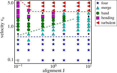
Figure 3: Phase diagram at high $\tau_{\mathrm{flip}}=100$ as a function of coupling $J$ and of active driving $v_{0}$. We observe a low $v_{0}$ phase with four $+1/2$ defects (blue stars, pale blue stars) which gives way to an intermediate set of band states with either merging defects (turquoise upright triangles) or $+1/2$ defects fully merged into two $+1$ defects at low $J$ (green circles). This phase is succeeded by turbulence above a threshold $v_{0}$ (red sideways triangles). At low $J$, a folding instability in the band shapes appears as driving increases (purple squares). Some states defied classification (black dots). The coloured lines are guides to the eye representing the phase boundaries.

III Characterising dynamical patterns and defect structures

In this section we briefly outline the methods used to analyse the results of our Brownian dynamics simulations. A summary of our method for identifying and tracking defects using a tessellation method in the presence of density fluctuations is given in Appendix A.

III.1 Mean-square displacements

To compute the mean squared displacement (MSD) of the defects, we used geodesic distances, i.e. the minimal distance along the great circle connecting the two positions in question. For two arbitrary points $\mathbf{r}_{i}$ and $\mathbf{r}_{j}$ on the $2-$sphere, we have

$$d_{ij}=R\arccos\left(\frac{\mathbf{r}_{i}}{R}\cdot\frac{\mathbf{r}_{j}}{R}\right).$$ (2)

Then the MSD is computed as

$$\text{MSD}(\delta t)=\langle d(t+\delta t)d(t)\rangle_{t,\text{defects}}.$$ (3)

Tracking was not always successful, especially at larger $v_{0}$, and we excluded trajectories with too many outliers from the MSD computations. For smaller numbers of outliers, we employed an error-correction algorithm that interpolates the outlier position from the previous and next correctly tracked points. The scaling of the MSD as MSD $\sim t^{\alpha}$ allowed us to identify diffusive ($\alpha=1$) and persistent $(\alpha>1$) regimes, and to compute the diffusion coefficients of defect motion (Fig. 4).

III.2 Pair angles

We define the pair angle between defects located at $\mathbf{r}_{i}$ and $\mathbf{r}_{j}$ as

$$\theta_{ij}=\arccos\left(\frac{\mathbf{r}_{i}}{R}\cdot\frac{\mathbf{r}_{j}}{R}\right).$$ (4)

For the tetrahedron the pair angles are all $\theta_{ij}=109.47^{\circ}$, while in an alternative flat configuration seen in Ref. Keber et al. (2014), four $90^{\circ}$ defects and two $180^{\circ}$ defects emerge, giving a mean pair angle $\langle\theta_{ij}\rangle=120^{\circ}$. We used $\langle\theta_{ij}\rangle$ to identify oscillations in Fig. 5. The $+1$ defects of the band state are nearly separated by $180^{\circ}$, and in the merging state, pairs of $+1/2$ defects approach each other. Pair defect angle distributions are shown in Fig. 6a, c.

III.3 Angular profiles

In the band state, a density profile emerges with bald spots at the poles and greater density at the equator. In parallel, the director field shows a systematic inclination towards the equator. Both effects are due to curvature-induced forces Sknepnek and Henkes (2015). We reoriented configurations with the pole axis along $\mathbf{z}$ as follows. We first computed an estimate $\mathbf{z}_{\text{Ine}}$ of the axis $\mathbf{z}$ from the eigenvector associated to the smallest eigenvalue of the inertial tensor $\hat{I}=\sum_{i}\mathbf{r}_{i}\times\mathbf{r}_{i}$. Then we determined a $\pm 1$ orientation for each velocity vector $\mathbf{v}_{i}$ on the basis that $\mathbf{r}_{i}\times\mathbf{v}_{i}$ is largely either parallel or antiparallel to $\mathbf{z}_{\text{Ine}}$, and finally computed

$$\mathbf{z}=\sum_{i}\mathbf{r}_{i}\times\text{orient}(\mathbf{v}_{i})$$ (5)

and normalised it. The density profiles in Fig. 6b, d and the orientation profile of the director $\alpha_{i}=\arccos(\mathbf{n}_{i}\cdot e_{\phi})$ in Fig. 6a have been averaged over all snapshots of several runs.

IV Results

We have studied spherical vesicles of radii $R=5-50$ for packing fraction $\phi=1$, corresponding to full coverage of the sphere and $10^{2}-10^{4}$ agents. Results reported here are for $R=30$, unless stated otherwise. All our simulations are in a steady-state, in the sense that they have relaxed from an initial random configuration. We study both the fast dynamics that immediately follows the relaxation to the steady state by integrating Eqs. (1) for a total of $1.5\times 10^{3}$ time units with time step $\delta t=10^{-3}$ using a standard Euler algorithm, and the dynamics at long times with $\delta t=0.05$ for a total integration time of up to $10^{5}$ time units.

In Fig. 1, we show the succession of states obtained with increasing activity $v_{0}$. As required by the Poincaré-Hopf theorem Frankel (2011), a nematic field on the surface of a sphere always contains topological defects with total charge $2$. This can be satisfied by two $+1$ defects at the poles of the sphere, or four $+1/2$ defects at the corners of a tetrahedron, or else by a turbulent state with many defects of both positive and negative charges, but adding up to a net charge of $+2$. The tetrahedral arrangement is the ground state configuration for a nematic with equal bend and splay Frank constants Nelson (2002); Shin et al. (2008). In the presence of activity the rules governing conservation of topological charge are of course unchanged, but defects often become dynamical entities that move with actively driven flows. At low activity $v_{0}$ we obtained a texture of four well-separated $+1/2$ disclinations, as shown in Fig. 1a. The four defects, however, are not static, but move either diffusively or, at long times, in an oscillatory fashion. At larger values of activity, pairs of $+1/2$ defects are pushed towards opposite poles (Fig. 1b) and eventually merge resulting in a configuration of two $+1$ defects at the poles, with a band of nematic wrapping around a great circle (Fig. 1c). Agents move within the band, with approximately equal fractions moving in clockwise and counterclockwise directions, so that nematic order is maintained with no mean flow. The “bald spots” at the poles can be interpreted as the cores of very large defects. The width of the band increases when lowering the alignment coupling $J$, as observed in polar systems Sknepnek and Henkes (2015). At even higher activity and sufficiently low alignment $J$, the band becomes unstable to bend deformations (Fig. 1d and Fig. 8) and one observes a complex folding dynamics, associated with sorting of particles into unidirectional lanes. Finally, upon further increase of $v_{0}$ the system exhibits turbulent-like flows with proliferation of topological defects (Fig. 1e), akin to that observed in planar systems.

We proceed to classify the various dynamical states depicted in Fig. 1 using the tools and methods discussed in previous section and the defect tracking algorithm outlined in Appendix A. By combining all of these results, we are able to map the complex dynamical states observed in the simulations in the phase diagram shown in Fig. 3.

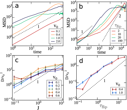
Figure 4: Mean square displacements (MSDs) of defects, and diffusion coefficients. (a) Four representative MSD trajectories of $+1/2$ defects as a function of $v_{0}$ for $J=1.0$ and $\tau_{\mathrm{flip}}=100$. From bottom to top: diffusive motion at low $v_{0}$ becomes superdiffusive in regions with oscillations, then subdiffusive in the merging state, and close to diffusive again in the folding state. (b) The long-time MSD for oscillating systems at $J=0.1$ and $v_{0}=0.4$ becomes nearly persistent at different $\tau_{\text{flip}}$. (c) Diffusion coefficient $D$ obtained from fits to the MSD, as a function of $J$ and scaled by $v_{0}^{2}$ for $\tau_{\mathrm{flip}}=100$. (d) Scaled diffusion coefficient $D/v_{0}^{2}$ as a function of $\tau_{\mathrm{flip}}$.

IV.1 Four-defect state

The four defects are generally motile on the sphere, as shown in Fig. 1 that displays the stereographic projections of their trajectories, with the only exception of the region of very low $v_{0}$ and $J$ where the system is effectively jammed (pale blue stars in the phase diagram Fig. 3 in a state akin to the one reported by Fily, et al. Fily et al. (2014) and by Janssen, et al. on the sphere Janssen et al. (2016)). To analyse the defect configuration and their dynamics we have examined the histogram of the angles $\theta_{ij}$ of defect pairs (Fig. 6a) and their mean-square-displacements (Fig. 4). We uncover two distinct regimes. At intermediate times, but long after settling into a long-lived steady state, the pair angle distribution is unimodal and peaked around $\theta=109^{\circ}$ corresponding to a tetrahedral configuration. In this regime, the MSD of the defects is diffusive (Fig.  4a) with a diffusion coefficient that scales as $D\sim v_{0}^{2}\tau_{\text{flip}}$ as expected for particles self-propelled at speed $v_{0}$ with noisy flips of their direction of self-propulsion at rate $\tau_{\text{flip}}$. The diffusion rate also grows linearly with the alignment rate $J$, suggesting a scaling $D=v_{0}^{2}\tau_{\text{flip}}f(J\mu k)$, with $f(x)\sim x$ at small $x$. We note that in this regime the local flow and pressure fields are dominated by fluctuations (see Fig. S2 in SI ), and we conjecture that the diffusive defect dynamics arises because defects are carried along by the strongly fluctuating flows. With increasing activity the distribution of pair angle broadens, but remains unimodal, and the MSD begins to cross over to superdiffusive behaviour at long times. Similar superdiffusive scaling was obtained by Shi and Ma for tapered rods Shi and Ma (2013) in the plane.

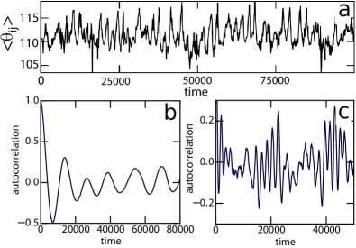
Figure 5: Oscillations of the defects at long times, for $v_{0}=1.0$, $J=0.1$ and $\tau_{\text{flip}}=1.0$: (a) mean pair angle $\langle\theta_{ij}\rangle$; (b) autocorrelation function of individual defect trajectories, showing a single oscillation period of $T\approx 10000$; (c) autocorrelation function of the mean pair angle, showing a superposition of several frequencies, with the fastest mode characterised by a period $T_{m}\approx 2000$.

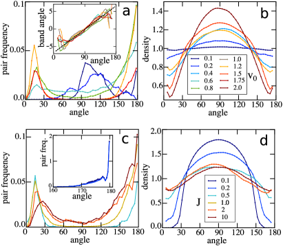
Figure 6: Emergence of the band state as seen from the distribution of defect pair angles (a-c) and the density profile (b-d). (a) At $J=1$, with increasing $v_{0}$, the pair angle distribution evolves form unimodal with a single central peak ($v_{0}=0.1$) to bimodal with growing peaks close to $0^{\circ}$ and $180^{\circ}$ ($v_{0}=0.6-1.5$). The inset shows the inclination of the direction of self-propulsion given by the director field $\mathbf{n}$ relative to the equator as a function of latitude. The black dashed line has a slope of $0.07$. (b) The corresponding density profiles evolve from homogeneous to banded. (c) For $J=0.5-10$, at $v_{0}=1.0$, the distribution peaks of the merging state shift inwards. Inset: For $J=0.1-0.2$, the two $+1$ defects are nearly at opposite poles. (d) In the corresponding density profile the bald spots at the poles disappear.

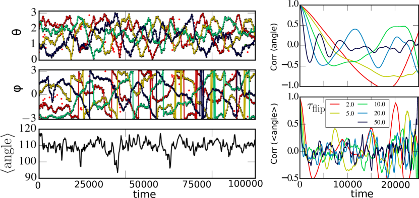
Figure S4: Oscillations at larger flip times $\tau_{\text{flip}}=2-50$ for $v=0.4$ and $J=0.1$ compared to Fig. 5 of the main text. In the left three panels, we show the defect trajectories in polar coordinates (top two panels), and the mean angle $\langle\theta_{ij}\rangle$ (bottom panel) for $\tau=50$. The right two panels show the defect trajectory autocorrelations (top) and the mean angle autocorrelations (bottom). The oscillations frequency increases with $\tau_{\text{flip}}$ in the range shown.

At very long times the defect dynamics becomes superdiffusive with a largest exponent of approximately $\alpha\approx 1.5$, and we observe oscillations akin to those reported in the experiments of Keber,et al. Keber et al. (2014), albeit only for specific parameter combinations. In Fig. 4b, we show the MSD trajectories over the full simulation time range in such a regime (corresponding to Fig. S4 of SI ). We analyse the oscillations in Fig. 5 (see also supplementary movie M1). The mean pair defect angle (panel a) oscillates between approximately $109^{\circ}$ and $115^{\circ}$ and the oscillations are less regular than those reported in the experiment of Keber et al. and in analytical Khoromskaia and Alexander (2016) and numerical Alaimo et al. (2017) treatments, where the mean angle oscillates between $109^{\circ}$ and $120^{\circ}$, clearly reflecting oscillations between tetrahedral and planar defect configurations. To quantify the angular periodicity we have evaluated the autocorrelation function of individual defect trajectories (panel b) and of the mean pair angle (panel c). Both display clear oscillatory behaviour, but the individual defect dynamics has a single oscillation period of $T\approx 20000$, while the mean angular dynamics is faster and controlled by several superimposed modes, with the fastest one oscillating at $T_{m}\approx 2000$. For $v_{0}=1.0$, $T$ increases with $\tau_{\mathrm{flip}}$ in the range sandwiched between frozen and band states. In Fig. S4 in SI , we show a corresponding analysis for $v=0.4$, where oscillations appear at much higher values of $\tau_{\mathrm{flip}}=10-50$. It is worth noting that we did not observe oscillations at any $J>0.1$, and we speculate that for larger $J$ the relaxation time $1/J$ of the director field is too fast for the flow field to coherently respond to it, so that again fluctuations dominate the dynamics.

IV.2 Band formation and merging defects

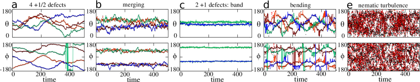
Figure S3: Defect tracks as a function of time for the same simulation runs as the stereographic projections in Fig. 1 of the main text. a: Four defects for $v_{0}=0.4$ and $J=1$, b: merging defects for $v_{0}=1.2$ and $J=2$, c: band state for $v_{0}=1.2$ and $J=0.1$, d: bending bands for $v_{0}=2.5$ and $J=0.1$, e: active turbulence for $v_{0}=5$ and $J=5$.

As $v_{0}$ increases,we observe the emergence of a nematic band wrapped around an equator that is chosen through spontaneous symmetry breaking (see Fig. 1b,c). The four $+1/2$ defects are pushed towards the poles, where they either form two nearly stationary trapped defect pairs (Fig. 1b’ and Fig. S3b) or merge into two fully stationary $+1$ defects (Fig. 1c’ and Fig. S3c). This configuration has also been seen in the experiments of Ref. Keber et al. (2014). The band state strongly resembles the band found in polar systems Sknepnek and Henkes (2015). It occurs because active particles are driven by curvature to move along geodesics, corresponding to great circles on a sphere. This effect is counterbalanced by repulsive interactions, resulting in the emergence of a finite-width band. Recent work by one of us Shankar et al. (2017) has also shown that the spontaneous emergence of bands wrapping around the equator is a generic properties of active polar fluids that arises from the interplay spontaneous flow and curvature. In our nematic system the band forms only for sufficiently long $\tau_{\text{flip}}$ ($\tau_{\mathrm{flip}}\geq 50$) when the system can support long-lived local polar flows that break the symmetry. Note that such bands are indeed seen in microtubule suspensions, where the defect structure shows clear nematic symmetry. In Fig. 6 we examine the emergence of the band by looking at the evolution of the defect pair angle distribution (Fig. 6a) and the density profile (Fig. 6b) with increasing $v_{0}$. The distribution of pair angles evolves from unimodal for $v_{0}=0.1-0.2$ corresponding to a fluctuating tetrahedral arrangement of four defects smeared-out by increasing diffusive motion to a bimodal one with peaks close to the location of opposing poles when the defects merge and the band state emerges. Meanwhile the density profile (Fig. 6b) evolves from practically uniform to a distinct peak that continuously grows with $v_{0}$, because the curvature-induced force that drives band formation is proportional to $v_{0}$ Sknepnek and Henkes (2015). A similar behaviour is obtained by decreasing $J$ for fixed $v_{0}$ (Fig. 6c,d). For low $J=0.1-0.2$, we always observe a band state with two $+1$ defects (inset to Fig. 6c), and a very peaked density profile appears, with bald spots at the poles. At higher $J$, this gradually gives way to a nematic band with unmerged pairs of defects at the poles and the first peak position gradually shifts to larger angles and the whole distribution broadens (Fig. 6c). We can explain this in part by noting that the defect core energy scales $\sim J$ when approximated by a single-constant Frank free energy Chaikin and Lubensky (2000) and so merging two $+1/2$ defects to form a $+1$ costs more energy at higher $J$. We see only slightly peaked density profiles for $J\geq 0.5$ (Fig. 6d). The tendency of active agents to move along geodesics is confirmed by examining the angle between the direction $\mathbf{n}$ of self-propulsion relative to the equator Sknepnek and Henkes (2015). The angle profile across a set of bands as a function of latitude is shown in the inset of Fig. 6c. The slope $\approx 0.07$ for the growth of the inclination of $\mathbf{n}$ with latitude is much shallower than in the polar case for the same $J$, consistent with the suppressed appearance of nematic bands as compared to polar ones at high $v_{0}$. Finally, in Sknepnek and Henkes (2015) we derived an effective profile for the polar band density. We show in SI that this also provides a good fit for the density profile of nematic bands.

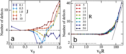
Figure 7: (a) Number of defects of any charge as a function of $v_{0}$ and $J$ for $R=30$. At low $v_{0}$, all curves converge to the equilibrium ground state with four $+1/2$ defects. As the driving is increased, the low $J$ systems develop a band state with two $+1$ defects. At the highest driving, the systems transition to a turbulent nematic state; lower $J$ delays onset of turbulence. (b) Defect scaling as a function of sphere radius for $J=10$. The onset of turbulence scales as $v_{0}R$. The dashed diagonal line has a slope of 2.

IV.3 Transition to turbulence

As even larger activity $v_{0}$, the system transitions to an active turbulent state, where pairs of $\pm 1/2$ defects are spontaneously created (Fig. 1e’ and Fig. S3e). In Fig. 7 we show the mean number of defects $N$ on the sphere regardless of their charges. We identify $N>4$ as the onset of turbulence.

The turbulent regime displays strong patterns of polar flow, consisting of lanes of particles moving in the same direction, as evident from Fig. 1e. We estimate that in our confined system the transition to turbulence occurs when the spacing $l_{\alpha}$ between defects becomes comparable to the sphere radius $R$. In hydrodynamic models in two spatial dimensions, the spacing between defects in the turbulent regime is expected to scale with the active stress $\alpha$ as $l_{\alpha}\sim\alpha^{-1/2}$ Giomi et al. (2013). By symmetry nematic activity is controlled by $v_{0}^{2}$. Assuming that the nematic stiffness is proportional to $J$, we estimate $\alpha\sim v_{0}^{2}J$. We then estimate that the transition to turbulence will occur when we can accommodate $N$ defects of mean separation $\ell_{\alpha}$ on the surface of the sphere, i.e., $N=4\pi R^{2}/l_{\alpha}^{2}$. This gives a prediction for the transition to turbulence as

$$N\sim(Rv_{0})^{2}J>4\;.$$ (6)

This form gives a very good scaling collapse of the observed number of defects for $J=10$ where there is no band state (Fig. 7b).

IV.4 The bending state

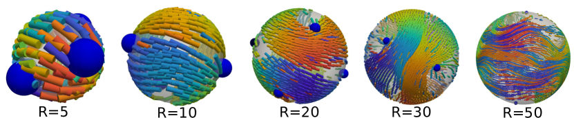
Figure S5: Bending states as a function of system size. This is an intermittent state which appears for only some of the simulation runs / part of a simulation run. For $\tau_{\text{flip}}=100$, the bending state disappears for $R\geq 50$. All systems are at $J=0.1$, and we have $v_{0}=1.0$ for $R=5$, and $v_{0}=3.0$ for $R=10-50$.

At low values of $J$, as already noted, the transition to turbulence is delayed. Instead, we observe an intriguing state, where the band that forms at intermediate $v_{0}$ develop a bending instability (Fig. 1d and Fig. 8). This is indeed seen in the experiments of Keber,et al. Keber et al. (2014) and we have also observed it in the polar case Sknepnek and Henkes . It is tempting to speculate that on a sphere this “bending of the bands” may provide a generic route to the spatiotemporal chaos of the turbulent state, but a more quantitative analysis beyond the scope of the present work will be required to substantiate this idea. Like in the experiment, the bending is intermittent: it is not seen in all runs for a given set of parameters, and it can both appear and disappear in a given simulation. The instability occurs via the mechanism described pictorially in Fig. 8. It is energetically favourable for the two $+1$ defects that sit at the poles in the band state to split into four $+1/2$ defects Shin et al. (2008) because by doing so they can lower the total core energy of the configuration. At low $J$, the elastic energy for bending a circulating band is low, and a bending instability can be triggered by the finite size of the sphere. This occurs when the persistence length of the nematic, $\xi=v_{0}\tau_{\mathrm{flip}}$, is comparable to the sphere circumference, so that agents can perform a full directed circulation around the sphere before reversing, resulting in lane formation and polar flows (see Fig. S2 in SI ). The interplay between curvature, polar flow and steric effects then drives such an instability, similar to a Rossby wave or a garden hose instability Batchelor (2000). The lowest mode of oscillation of the “bent band” at maximum amplitude is compatible with the tetrahedral defect state of the nematic, as the large meander of the band includes one $+1/2$ defect in every bend, resulting in a configuration with opposing streams touching at the front and the back of the sphere, as sketched out in Fig. 8. In Fig. S5 in SI , we show the evolution of the bending state with sphere radius $R$. Like in experiment, bending is observed only for sufficiently small systems where $v_{0}\tau_{\mathrm{flip}}\geq R$.

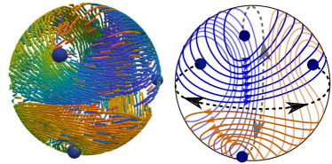
Figure 8: Bending of the band at high activity and low alignment. The high persistence lengths favour polarity sorting, leading to one-directional polar flow. The $+1$ defects of the band split into pairs of $+1/2$ defects that are gradually pushed to the vertices of a tetrahedron. Left: Simulation snapshot at $J=0.1$, $v_{0}=3.0$. Right: Schematic drawing of the topological state.

V Conclusions

In this paper we presented results of detailed numerical simulations of a model of self-propelled agents with nematic alignment confined to move on the surface of a sphere. We developed algorithms for automatic detection and tracking of topological defects, which allowed us to characterise a series of emergent collective motion patterns and construct a detailed phase diagram. The onset of these patterns can be understood using ideas from liquid crystal theory, topology, and the study of active nematics in flat space. Our work provides a systematic framework for the experimental results of Keber, et al. Keber et al. (2014). Most of the states observed here have been seen in the experiment at different sphere radii $R$ and ATP concentrations. We believe that our phase diagram Fig. 3 will be especially useful. In contrast to the two existing hydrodynamic models Keber et al. (2014); Khoromskaia and Alexander (2016), we can access high-activity states with large density fluctuations, which are highly experimentally relevant as bands form there.

A full continuum analytical theory of this system is lacking at present. Taking the proper hydrodynamic limit of agent-based active nematic models at high densities is complex Gao et al. (2015). Continuum active nematic theories rely on the presence of extensile or contractile active stresses, but the origin of such stresses is unclear in particle-based models where activity is most naturally introduced as self-propulsion. In order to obtain nematic behaviour one has to introduce a flipping time scale $\tau_{\mathrm{flip}}$ of the director. As we showed here, the onset of most collective motion patterns is sensitive to this time scale. Furthermore, we showed that while the behaviour predicted by continuum theory emerges at large scales, there is an intermediate scale in which the non-universal microscopic details of the model cannot be ignored and can actually dominate the physics. An important consequence is that defect motion in self-propelled active nematics, as shown here and in Shi and Ma (2013), is very slow, only mildly superdiffusive, and dominated by local fluctuations. In contrast, in locally extensile systems such as DeCamp et al. (2015); Alaimo et al. (2017) a local flow field does seem to naturally emerge. Despite these limitations, we argue that agent-based models can provide valuable insight into the behaviour of active nematics.

One other hurdle to a direct comparison with experiment is that we have simulated disks, not polymers. Recent planar simulations of active polymer melts by two of us show that hairpin bends in the filaments (which are also apparent in experiment) are strongly implicated in the defect dynamics Prathyusha et al. (2016). In the future, for greater experimental relevance, we plan to directly simulate active polymers with an extensile activity mechanism. Preliminary results show that defect motion and oscillations dominate the motion, but only if all locally polar parts of the dynamics are suppressed. Finally, it would be desirable to move away from the dry limit and explicitly include hydrodynamic effects.

VI Acknowledgements

The authors would like to acknowledge many valuable discussions with Mark Bowick, Daniel L. Barton, and Prathyusha K. R. This collaboration was made possible by a travel grant from the Northern Research Partnership (NRP) Fund. RS acknowledge support by UK BBRSC (grant BB/N009789/1) and SH acknowledges support by the UK BBSRC (grant BB/N009150/1). MCM was supported by the US National Science Foundation through awards DMR-1609208 and DGE-1068780 and by the Syracuse Soft Matter Program.

Appendix A Identifying and tracking topological defects

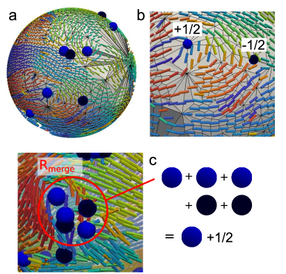
Figure 9: (a) Example of the contact network and its dual (grey polygons) on a sphere with substantial density fluctuations. We use the same colour convention for the discrete director field as in Fig. 1. (b) Zoom-in onto a pair of a positive and a negative $1/2$ defects. (c) Illustration of the merging technique for spots with local disorder. The five $\pm 1/2$ defects within $R_{\text{merge}}$ combine into one $+1/2$ defect.

We begin by discussing the algorithm used to identify and track topological defects. The identification of the defects is not completely straightforward due to large density fluctuations that accompany some of the collective motion patterns, where one has to distinguish between a defect and a bald spot. In order to discriminate between the two, we implemented a generalised computation of the winding number. For each agent we constructed a network of all of its neighbours within a cutoff distance, i.e. the contact network. For systems with large density fluctuations it is not practical to impose a predefined cutoff, and instead we iteratively adjusted the cutoff distance until each agent had at least three neighbours. We then used the contact network to construct a polygonal tessellation of the sphere. Finally, we connected geometric centres of each of those polygons to construct the dual lattice. Compared to, e.g., a Voronoi diagram and its dual Delaunay triangulation, our method has the advantage that it generalises to any orientable surface. As a result of this construction, each vertex of the dual lattice is in the centre of a polygonal loop with the nematic director, $\mathbf{n}$, or velocity, $\mathbf{v}$, assigned to each of its corners. Each loop then acts as a discrete integration path for $\mathbf{n}$ or $\mathbf{v}$. Finally, we projected the field vectors onto the local tangent plane (plane of the polygonal loop), and integrated angle differences between two consecutive vertices in the counterclockwise direction around the contour, giving us the half-integer values of the topological charges for each loop centre. In Fig. 9a-b we show examples of $\mathbf{n}$-fields, tessellations and defects. Defects together with their charges are shown in Fig. 1 and Fig. 8. Determining the total number of defects allows us to easily identify the transition to turbulence (Fig. 7).

We then tracked defects between consecutive snapshots of a simulation by matching defects of a given charge with the nearest defect with the same charge in the previous frame. To reduce spurious tracking errors due to proliferation of defect clusters at spots with local disorder, we first merges all defect charges within a radius $R_{\text{merge}}=5\sigma$, as shown in Fig. 9c. We were able to track $+1/2$ defects in the four defect, merging and bending states, and $+1$ defects in the band state. We did not attempt to track $-1/2$ defects, or defects in the turbulent state. Using spherical coordinate system, position of each defect was identified by a unique $\theta$ and $\phi$. Fig. 1 shows the stereographic projections of representative defect trajectories for the various states with the defects tracked in different colours. The corresponding trajectories in the sphere are shown in Fig S2 of SI .

Dynamical patterns in active nematics on a sphere: Supplementary information

Band profiles

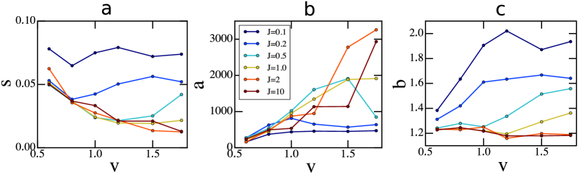
Figure S1: Results of the fits of the angle and density profiles to the polar band theory.

In Ref. [23] of the main text, we derived an effective equation for the band density

$$\rho(\theta)=a\left[(\sin s\theta\!-\!\sin s\theta_{m})\right]+b,\quad\theta\in[\theta_{m},\pi-\theta_{m}]$$ (S1)

$$\rho(\theta)=0\quad\text{otherwise,}$$

where $a=\frac{1}{2R}\left[\frac{R}{2\sigma}\right]\frac{v_{0}}{\mu ks}$ and $b/a=\frac{2\sigma}{R}s\cos s\theta_{m}+\frac{1}{a}$ for the polar case (note that in [23] , we chose $\theta=0$ at the equator). Eq. (S1) describes a sine profile symmetric about the equator between two band edges located at $\theta_{m}$ and $\pi-\theta_{m}$. Here $s$ is the effective coupling strength between the active force direction $\mathbf{n}$ and the angle from the equator. It can be measured as the slope of the $\mathbf{n}$-angle profiles $\alpha(\theta)$. An example of such a profile in the full band state at $J=0.1$ is in the inset of Fig. 6a of the main text. The slope is clearly visible, though much shallower than in the polar case. The large deviations are in the edge regions where the density drops to zero.

In Figure S1, we fit equation S1 to the nematic bands. In panel a, we show the $s$ from fits to the slope in the middle parts of the profiles. Like in the polar case, $s$ decreases with $J$ from a maximum of $s=0.07$ at $J=0.1$ until it reaches a plateau at $s\approx 0.03$ for $J\geq 0.5$. This is consistent with the scaling of the density profiles shown in Fig. 6b-d of the main text. The low values of $s$ are also consistent with the delayed appearance of the band state in the nematic system compared to the polar one. We also notice that unlike for the polar case, for the nematic case $s$ depends on $v_{0}$: After an initial peak that coincides with the first appearance of the bands, $s$ decreases until it hits a $J$-dependent plateau value. Finally, in panel b and c we show the values of $a$ and $b$ extracted from fits to eq. S1 using the $s$ from panel a. Consistent with the polar case and the increasingly peaked density profiles that we observe, $a$ increases with $v_{0}$, though not in the linear fashion of the analytical prediction.

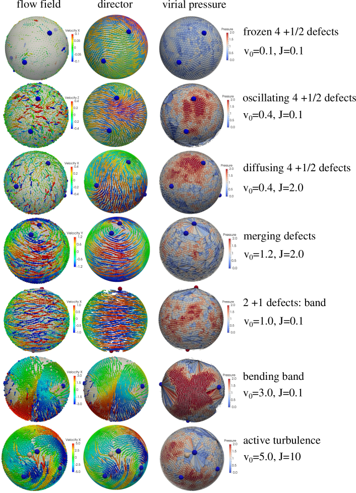
Figure S2: Flow fields (left), nematic director fields (middle) and pressure (right) in the different dynamical patterns that we observe. Here both flow field and nematic field have been colored by the same component of motion as indicated in the caption for the velocity. The limits on the velocity color bars correspond to $(-v_{0},v_{0})$. For the virial pressure, we compute $p_{i}=\sum_{j}\mathbf{r}_{ij}\cdot\mathbf{F}_{ij}/A_{i}$ for each agent. Here the sum runs over the contact neighbors $j$ of $i$, and $A_{i}$ is the area of the tile belonging to $i$ computed from the dual to the contact network. On the image, each tile has been colored by its pressure. As in Fig. 1 of the main text, $+1/2$ defects are blue, $-1/2$ defects are tan, and $+1$ defects are red.

References

- Marchetti et al. (2013) M. Marchetti, J. Joanny, S. Ramaswamy, T. Liverpool, J. Prost, M. Rao, and R. A. Simha, Rev. Mod. Phys. 85, 1143 (2013).
- Ramaswamy (2010) S. Ramaswamy, The Mechanics and Statistics of Active Matter 1, 323 (2010).
- Vicsek et al. (1995) T. Vicsek, A. Czirók, E. Ben-Jacob, I. Cohen, and O. Shochet, Phys. Rev. Lett. 75, 1226 (1995).
- Voituriez et al. (2005) R. Voituriez, J.-F. Joanny, and J. Prost, EPL (Europhysics Letters) 70, 404 (2005).
- Simha and Ramaswamy (2002) R. A. Simha and S. Ramaswamy, Physical review letters 89, 058101 (2002).
- Narayan et al. (2007) V. Narayan, S. Ramaswamy, and N. Menon, Science 317, 105 (2007).
- Chaté et al. (2006) H. Chaté, F. Ginelli, and R. Montagne, Phys. Rev. Lett. 96, 180602 (2006).
- Hatwalne et al. (2004) Y. Hatwalne, S. Ramaswamy, M. Rao, and R. A. Simha, Physical review letters 92, 118101 (2004).
- Marchetti (2012) M. C. Marchetti, Nature 491, 340 (2012).
- Sanchez et al. (2012) T. Sanchez, D. T. Chen, S. J. DeCamp, M. Heymann, and Z. Dogić, Nature 491, 431 (2012).
- Saw et al. (2017) T. B. Saw, A. Doostmohammadi, V. Nier, L. Kocgozlu, S. Thampi, Y. Toyama, P. Marcq, C. T. Lim, J. M. Yeomans, and B. Ladoux, Nature 544, 212 (2017).
- Kawaguchi et al. (2017) K. Kawaguchi, R. Kageyama, and M. Sano, Nature (2017).
- Yang et al. (2014) X. Yang, D. Marenduzzo, and M. Marchetti, Physical Review E 89, 012711 (2014).
- Fily et al. (2016) Y. Fily, A. Baskaran, and M. F. Hagan, arXiv preprint arXiv:1601.00324 (2016).
- Sato et al. (2009) T. Sato, R. G. Vries, H. J. Snippert, M. Van de Wetering, N. Barker, D. E. Stange, J. H. Van Es, A. Abo, P. Kujala, P. J. Peters, et al., Nature 459, 262 (2009).
- Collinson et al. (2002) J. M. Collinson, L. Morris, A. I. Reid, T. Ramaesh, M. A. Keighren, J. H. Flockhart, R. E. Hill, S.-S. Tan, K. Ramaesh, B. Dhillon, and J. D. West, Dev. Dyn. 224, 432 (2002).
- Keber et al. (2014) F. C. Keber, E. Loiseau, T. Sanchez, S. J. DeCamp, L. Giomi, M. J. Bowick, M. C. Marchetti, Z. Dogic, and A. R. Bausch, Science 345, 1135 (2014).
- Nelson (2002) D. R. Nelson, Nano Letters 2, 1125 (2002).
- Shin et al. (2008) H. Shin, M. J. Bowick, and X. Xing, Physical review letters 101, 037802 (2008).
- Giomi et al. (2013) L. Giomi, M. J. Bowick, X. Ma, and M. C. Marchetti, Phys. Rev. Lett. 110, 228101 (2013).
- Khoromskaia and Alexander (2016) D. Khoromskaia and G. P. Alexander, arXiv preprint arXiv:1608.02813 (2016).
- Alaimo et al. (2017) F. Alaimo, C. Köhler, and A. Voigt, arXiv preprint arXiv:1703.03707 (2017).
- Sknepnek and Henkes (2015) R. Sknepnek and S. Henkes, Phys. Rev. E 91, 022306 (2015).
- Shankar et al. (2017) S. Shankar, M. J. Bowick, and M. C. Marchetti, arXiv preprint arXiv:1704.05424 (2017).
- Ehrig et al. (2016) S. Ehrig, J. Ferracci, R. Weinkamer, and J. W. Dunlop, arXiv preprint arXiv:1610.05987 (2016).
- Gao et al. (2015) T. Gao, R. Blackwell, M. A. Glaser, M. Betterton, and M. J. Shelley, Physical review letters 114, 048101 (2015).
- Shi and Ma (2013) X.-q. Shi and Y.-q. Ma, Nature communications 4 (2013).
- Bertin et al. (2015) E. Bertin, A. Baskaran, H. Chaté, and M. C. Marchetti, Physical Review E 92, 042141 (2015).
- Cates and Tailleur (2015) M. E. Cates and J. Tailleur, Annu. Rev. Condens. Matter Phys. 6, 219 (2015).
- Szabó et al. (2006) B. Szabó, G. Szöllösi, B. Gönci, Z. Jurányi, D. Selmeczi, and T. Vicsek, Phys. Rev. E 74, 061908 (2006).
- Henkes et al. (2011) S. Henkes, Y. Fily, and M. C. Marchetti, Phys. Rev. E 84, 040301 (2011).
- DeCamp et al. (2015) S. J. DeCamp, G. S. Redner, A. Baskaran, M. F. Hagan, and Z. Dogic, Nature materials 14, 1110 (2015).
- Frankel (2011) T. Frankel, The geometry of physics: an introduction (Cambridge University Press, 2011).
- Fily et al. (2014) Y. Fily, S. Henkes, and M. C. Marchetti, Soft matter 10, 2132 (2014).
- Janssen et al. (2016) L. Janssen, A. Kaiser, and H. Löwen, arXiv preprint arXiv:1611.03528 (2016).
- (36) “See supplemental material at [url will be inserted by publisher] for movies of the motion patterns.” .
- Chaikin and Lubensky (2000) P. Chaikin and T. Lubensky, Principles of Condensed Matter Physics (Cambridge University Press, 2000).
- (38) R. Sknepnek and S. Henkes, “Polar and nematic fields on orientable surfaces, in preparation,” .
- Batchelor (2000) G. K. Batchelor, An introduction to fluid dynamics (Cambridge university press, 2000).
- Prathyusha et al. (2016) K. Prathyusha, S. Henkes, and R. Sknepnek, arXiv preprint arXiv:1608.03305 (2016).