Sensitivity of directed networks to the addition and pruning of edges and vertices.

Abstract

We study the sensitivity of directed complex networks to the addition and pruning of edges and vertices and introduce the susceptibility, which quantifies this sensitivity. We show that topologically different parts of a directed network have different sensitivity to the addition and pruning of edges and vertices and, therefore, they are characterized by different susceptibilities. These susceptibilities diverge at the critical point of the directed percolation transition, signaling the appearance (or disappearance) of the giant strongly connected component in the infinite size limit. We demonstrate this behavior in randomly damaged real and synthetic directed complex networks, such as the World Wide Web, Twitter, the Caenorhabditis elegans neural network, directed Erdős-Rényi graphs, and others. We reveal a non-monotonous dependence of the sensitivity to random pruning of edges or vertices in the case of Caenorhabditis elegans and Twitter that manifests specific structural peculiarities of these networks. We propose the measurements of the susceptibilities during the addition or pruning of edges and vertices as a new method for studying structural peculiarities of directed networks.

I Introduction

Many real-world complex systems can be represented by directed complex networks. In this kind of network every edge between two interacting subjects can be directed, i.e., it goes in only one direction, and bidirected, i.e., it goes in both directions. Well-known examples are the World Wide Web (WWW) Broder et al. (2000), neuronal and metabolic networks Sporns et al. (2004); Barabási and Oltvai (2004), gene regulatory networks Lee et al. (2002); Liu et al. (2015), social networks, such as Twitter Kwak et al. (2010), the control network of transnational corporations Vitali et al. (2011), and many other complex systems Newman (2003); Dorogovtsev and Mendes (2002). A common feature of these complex systems is that they are developing by means of the addition of directed edges and vertices while diseases, injuries, random or targeted damages lead to the degradation of the network structure due to pruning of edges or vertices. For example, in the brain, neurogenesis (the creation of new nerve cells) and the formation of new synaptic connections, as well as the opposite process – pruning of synapses or neurons, are important mechanisms for the brain development Sporns et al. (2004); Bullmore and Sporns (2012), learning and memory Chklovskii et al. (2004); Brunel (2016), and sex-specific circuit development Oren-Suissa et al. (2016); Portman (2016), and for other brain functions. In contrast to neurogenesis, neurodegenerative diseases are accompanied by the loss of neurons or synapses and degradation of the brain networks Stephan et al. (2006); Palop and Mucke (2010); Benes et al. (2001). Twitter, a social network, is developing in a similar way, growing due to addition of new users and the formation of new connections Kwak et al. (2010). The structure of these directed networks plays a very important role in their functioning. The structure of a directed network is much more subtle and richer than the structure of its undirected version Broder et al. (2000); Newman et al. (2001); Dorogovtsev et al. (2001); Timár et al. (2017). In general, a directed graph consists of the giant strongly connected component $G_{S}$, which is a central core of the network, the sets $IN$ and $OUT$ of vertices playing the role of the incoming and outgoing terminals for $G_{S}$. There are also finite directed components $F$ (tendrils, tubes, and disconnected finite clusters). If in the initial state a network consists of isolated vertices and disconnected finite clusters, then the addition of directed edges leads to the appearance of $G_{S}$ at the critical point of the directed percolation transition. Edges can be added at random, as in the case of ordinary percolation, or by exploiting some optimization principle, for example, the Achlioptas process, as in the case of explosive percolation Achlioptas et al. (2009); Squires et al. (2013). In networks subjected to pruning of edges or vertices, $G_{S}$ disappears at the critical point below which the network disintegrates into a set of finite directed components and disconnected clusters. Taking into account the crucial role of $G_{S}$ in dynamics, functioning, and the propagation of information in directed complex networks, it is very important to develop methods that quantify the sensitivity of the networks to structural changes and signal the approaching of the critical transition. In physics, the sensitivity of a system to an applied field is quantified by the susceptibility, which characterizes the sensitivity of the order parameter to an applied field (see, for example, Stanley (1971)). The susceptibility diverges in the infinite size limit when a system under consideration approaches the critical point of a continuous phase transition. Thus the susceptibility not only quantifies the response of a system to an applied field but also signals the approaching of the phase transition. The generalized susceptibility was already discussed in the case of ordinary percolation Stauffer and Aharony (1994) and explosive percolation da Costa et al. (2010, 2014) in undirected complex networks. In the case of directed complex networks, the susceptibility was recently introduced in Timár et al. (2017). However, a relation between the susceptibility and the sensitivity of directed networks to the addition and pruning of edges or vertices was not yet studied. Since different network parts ($G_{S}$, $IN$, $OUT$, and $F$) have different topological properties, one can assume that these parts also differ in the sensitivity to the addition and pruning of edges or vertices and, therefore, they must be characterized by different susceptibilities. This problem has not yet been discussed in the literature.

In this paper, we study the response of directed networks to the addition and pruning of edges and vertices. We show that topologically different network parts ($IN$, $OUT$, $G_{S}$, and $F$) have different sensitivities to this kind of impact on the networks. These sensitivities are quantified by the different susceptibilities, which can be found by use of the two-point connectivity function characterizing whether any two vertices are connected by a directed path or not. Alternatively, we find the susceptibilities by analyzing statistics of individual out-components and in-components of vertices in $IN$, $OUT$, $G_{S}$, and $F$. We use these local characteristics for quantifying the response of the giant component $G_{S}$, $IN$, $OUT$, and the finite network components $F$ to the addition and pruning of edges or vertices. Using the generating function method, we find analytically the susceptibilities of uncorrelated random directed complex networks in the infinite size limit and demonstrate that the susceptibilities diverge at the critical point, signaling the percolation transition in these networks. Finally, we study numerically the susceptibilities of some real and synthetic directed complex networks subjected to random damage and show that these susceptibilities characterize the sensitivity of even small directed networks to damage and depend strongly on structural peculiarities of the directed networks.

II Structure of directed networks

In order to find the response of a directed network to the addition or removal of edges or vertices, we first need to know its structure. In this section we describe the common structural properties of directed graphs revealed in Broder et al. (2000); Newman et al. (2001); Dorogovtsev et al. (2001); Schwartz et al. (2002); Boguñá and Serrano (2005); Bianconi et al. (2008); Timár et al. (2017).

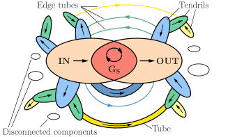
Figure 1: (Color online) Schematic view of the structure of a directed network. There are the giant strongly connected component $G_{S}$ (the core of the network), the sets $IN$ and $OUT$, the finite directed components $F$ [tendrils and tubes shown as domains of different colors, and disconnected finite clusters (open ovals)]. The union of these parts is the giant weakly connected component $G_{W}$. Tendrils belonging to the same layer have the same color. Edge tubes of different layers are shown in corresponding colors. Only three tendril layers are shown.

Directed networks have a hierarchical organization Broder et al. (2000); Newman et al. (2001); Dorogovtsev et al. (2001); Timár et al. (2017) and can be partitioned into topologically different parts (see Fig. 1): (i) the giant strongly connected component ($G_{S}$), which is a central core of the directed network, (ii) sets of vertices called $IN$ and $OUT$ that are connected to $G_{S}$, (iii) hierarchically organized finite directed components (tendrils and tubes) that are only connected to $IN$ and $OUT$ but not to $G_{S}$, and (iv) disconnected finite clusters. These parts have different topological properties. The definitions of these network parts were given in Broder et al. (2000); Newman et al. (2001); Dorogovtsev et al. (2001); Timár et al. (2017). Let us briefly review them. The giant strongly connected component $G_{S}$ is a subgraph in which every vertex can be reached from every other vertex by following directed edges. $OUT$ is a set of vertices that can be reached from the $G_{S}$ by following directed edges, but from which it is not possible to reach the $G_{S}$. $IN$ is a set of vertices from which the strongly connected component $G_{S}$ can be reached by following directed edges, but which can not be reached from the strongly connected component by following directed edges. Note that $IN$ and $OUT$ may appear only when $G_{S}$ appears. In some real directed complex networks, such as the neural network of Caenorhabditis elegans (C. elegans) Jarrell et al. (2012), the giant strongly connected component $G_{S}$ includes almost all vertices of the considered network (492 vertices among 495 vertices in C. elegans, see Sec. VII for more details), as a condition of its normal functioning Timár et al. (2017).

The union of the sets $G_{S}$ and $OUT$ is the giant out-component $G_{out}$ Dorogovtsev et al. (2001), i.e.,

$$G_{out}=G_{S}\cup OUT.$$ (1)

In turn, the union of $G_{S}$ and $IN$ is the giant in-component $G_{in}$ Dorogovtsev et al. (2001), i.e.,

$$G_{in}=G_{S}\cup IN.$$ (2)

The remaining part ($F$) of the graph $\mathcal{G}$ is the union of finite components including finite directed components $T$ (tendrils and tubes) and finite disconnected clusters $C$, i.e.,

$$F=T\cup C=\mathcal{G}\setminus(G_{S}\cup IN\cup OUT).$$ (3)

Tendrils and tubes in $T$ have a hierarchical, multilayer organization around $IN$ and $OUT$ Timár et al. (2017). They can exist only when $IN$ and $OUT$ are present in the network. The set of vertices $C$ is the union of all finite disconnected clusters $C_{\alpha}$, $\alpha=1,2,3,\dots$, i.e., ($C=C_{1}\cup C_{2}\cup C_{3}\dots$).

The giant weakly connected component $G_{W}$ is the union of $G_{S}$, $IN$, $OUT$, tendrils, and tubes, i.e.,

$$G_{W}=G_{S}\cup IN\cup OUT\cup T=\mathcal{G}\setminus C.$$ (4)

If we neglect the edge directedness, we find that the subgraph $G_{W}$ is the giant connected component of the undirected version of the graph $\mathcal{G}$. Note that $G_{W}$ can exist even if $G_{S}$, $IN$, and $OUT$ are absent in the network.

We also introduce a subgraph $G_{IO}$ as the union

$$G_{IO}\equiv G_{S}\cup IN\cup OUT=\mathcal{G}\setminus F.$$ (5)

We suggest that the size of $G_{IO}$ is the order parameter for the percolation transition in directed networks Timár et al. (2017). Note that in undirected networks, the size of the giant connected component (the undirected version of $G_{W}$) is the order parameter for the ordinary percolation. There are similarities between the topological structure of the order parameters $G_{IO}$ and the giant connected component (the undirected version of $G_{W}$) of an undirected network. The latter consists of the 2-core, i.e., the largest subgraph whose vertices have degree at least 2, and finite branches attached to this 2-core Dorogovtsev et al. (2008). In directed networks, $G_{IO}$ includes the subgraph $G_{S}$, whose vertices also have degree at least two (at least one incoming edge and at least one outgoing edge with vertices within the subgraph $G_{S}$). Vertices in $IN$ and $OUT$ form directed incoming and outgoing branches, respectively, attached to the $G_{S}$.

In the general case, any directed graph $\mathcal{G}$ can be written as the following union:

$$\mathcal{G}=G_{IO}\cup F=G_{W}\cup C=G_{S}\cup IN\cup OUT\cup T\cup C.$$ (6)

If there is no giant component $G_{S}$, the graph $\mathcal{G}$ consists of only finite directed components and finite disconnected clusters, i.e., $\mathcal{G}=F$.

If a directed network consists of only disconnected finite clusters then the addition of new directed edges results at first in the ordinary percolation transition into state in which the undirected version of this directed network has a nonzero giant connected component. Then, adding more directed edges, the network undergoes the directed percolation transition into a state with a nonzero giant strongly connected component $G_{S}$.

Let us characterize the network parts, i.e., $G_{S}$, $IN$, $OUT$, and the finite directed components, using the sizes of the individual in- and out-components of vertices $i$ Newman et al. (2001); Dorogovtsev et al. (2001); Timár et al. (2017). By definition, the in-component and out-component of vertex $i$ are the sets of vertices reachable by following edges either backwards or forwards from $i$, respectively. If vertex $i$ belongs to $F=T\cup C$ then it has finite in- and out-components, i.e., their sizes are of the order of $O(1)$ [i.e., $s_{in}(i),s_{out}(i)\propto O(1)]$. Vertices belonging to $G_{S}$ have equal sizes of in-components and equal sizes of out-components, namely, $s_{in}(i)=N(G_{in})-1$ and $s_{out}(i)=N(G_{out})-1$ for any $i\in G_{S}$. These individual components are giant, i.e., $s_{in}(i),s_{out}(i)\propto O(N)$. If $i\in IN$ then $s_{in}(i)\propto O(1)$ while $s_{out}(i)\propto O(N)$. If $i\in OUT$ then $s_{in}(i)\propto O(N)$ while $s_{out}(i)\propto O(1)$. Note that in general $s_{in}(i)$, as well as $s_{out}(i)$, are different for different $i$ in both $IN$ and $OUT$.

In Secs. V - VII we will study how the addition and pruning of edges and vertices affect the components of directed networks and their sensitivity to damage both below and above the directed percolation transition.

III Two-point connectivity function

Let us consider an arbitrary directed graph $\mathcal{G}$ of size $N(\mathcal{G})\equiv N$. In order to characterize the connectivity of the graph, we introduce a two-point connectivity function $C(i\rightarrow j)$ of vertices $i$ and $j$ as follow: (i) $C(i\rightarrow i)=1$; (ii) $C(i\rightarrow j)=1$ if there is a directed path from $i$ to $j$ (note that there can be more than one path). Otherwise, $C(i\rightarrow j)=0$. In general $C(i\rightarrow j)$ is asymmetric, $C(i\rightarrow j)\neq C(j\rightarrow i)$, since a directed path from $j$ to $i$ can be present while a directed path from $i$ to $j$ can be absent, and vice versa. The function $C(i\rightarrow j)$ is the generalization of the two-point correlation function of the one-state Potts model in undirected networks Wu (1982) to the case of directed networks. The two-point connectivity function $C(i\rightarrow j)$ is determined by the adjacency matrix $A_{ij}$. This relation can be written in the form

$$C(i\rightarrow j)=\Theta(\sum_{n=1}^{\infty}(A^{n})_{ij}),$$ (7)

at $i\neq j$. The theta-function $\Theta(x)$ is 1 if $x>0$ and zero otherwise. Let us also introduce the function,

$$C(i,j)\equiv C(i\rightarrow j)+C(j\rightarrow i)-C(i\rightarrow j)C(j\rightarrow i),$$ (8)

which is symmetric, i.e., $C(i,j)=C(j,i)$. Furthermore, $C(i,i)=1$ and $C(i,j)=1$ if there is a directed path from $i$ to $j$ or from $j$ to $i$, or in both directions. Otherwise, $C(i,j)=0$.

Using the function $C(i\rightarrow j)$, we can find the individual in- and out-components of every vertex $i$, which are defined as the sets of vertices reachable by following edges either backwards or forwards from $i$, respectively. The sizes $s_{in}(i)$ and $s_{out}(i)$ of these components are

$$s_{in}(i) = \sum_{j\in\mathcal{G}\backslash i}C(j\rightarrow i),$$ (9)

$$s_{out}(i) = \sum_{j\in\mathcal{G}\backslash i}C(i\rightarrow j),$$ (10)

$$s_{t}(i) = \sum_{j\in\mathcal{G}\backslash i}C(i,j),$$ (11)

where the sum is over all vertices $j\in\mathcal{G}$ except $i$. Here, $s_{t}(i)$ is the total number of vertices reachable by following edges both backwards and forwards from $i$. Using Eqs. (9) and (10), we find that the mean sizes $\langle s_{in}\rangle$ and $\langle s_{out}\rangle$ of the individual in- and out-components of a randomly chosen vertex are equal to each other:

$$\langle s_{in}\rangle \equiv \frac{1}{N(\mathcal{G})}\sum_{i\in\mathcal{G}}s_{in}(i)=\frac{1}{N(\mathcal{G})}\sum_{i\neq j\in\mathcal{G}}C(j\rightarrow i)$$ (12)

$$= \frac{1}{N(\mathcal{G})}\sum_{j\in\mathcal{G}}s_{out}(j)=\langle s_{out}\rangle.$$

In the general case we have $s_{t}(i)\leq s_{in}(i)+s_{out}(i)$ for vertices $i\in\mathcal{G}$ because there might be vertices that belong simultaneously to in- and out-components of vertex $i$ due to loops and bidirectional edges.

If we neglect the edge directness then the function $C(i\rightarrow j)$ becomes symmetric, $C(i\rightarrow j)=C(j\rightarrow i)=C(i,j)$. Note that in this case $C(i,j)=1$ if $i$ and $j$ belong to the same cluster $C_{\alpha}$. Therefore, according to Eq. (9), the total number $s_{t}(i)$ of vertices reachable from vertex $i$ equals $N(C_{\alpha})-1$ where $N(C_{\alpha})$ is the size the cluster $C_{\alpha}$ to which $i$ belongs.

Below we show that the two-point connectivity function $C(i\rightarrow j)$ is a very useful mathematical object for quantifying the response of a network to the addition and pruning of edge and vertices.

IV Susceptibility of directed networks

It is well known that the one-state Potts model is equivalent to the ordinary percolation model Stauffer and Aharony (1994) in undirected networks Kasteleyn and Fortuin (1969); Wu (1982). The Ising model is a particular case of the two-state Potts model. In the Ising model, the susceptibility, $\chi=dM/dH$, quantifies the sensitivity of the magnetization $M$ to an applied magnetic field $H$. The susceptibility is related with the irreducible two-spin correlation function $C(i,j)$ as follows:

$$\chi = \frac{1}{N}\sum_{i,j}C(i,j),$$ (13)

$$C(i,j) = \langle\sigma_{i}\sigma_{j}\rangle_{T}-\langle\sigma_{i}\rangle_{T}\langle\sigma_{j}\rangle_{T},$$ (14)

where $\langle\sigma_{i}\rangle_{T}$ stands for the averaging of spin $\sigma_{i}$ over the Gibbs ensemble (see, for example, in Parisi (1988)). The local magnetization is nonzero (i.e., $\langle\sigma_{i}\rangle_{T}\neq 0$) in the ordered phase at zero magnetic field. The zero-field susceptibility diverges at the critical point signaling a continous phase transition into the ordered phase.

In directed networks there are two connectivity functions, $C(i\rightarrow j)$ and $C(i,j)$, defined in Sec. III. Using the equivalence of the percolation model to the one-state Potts model, we introduce two susceptibilities $\chi_{d}$ and $\chi_{t}$,

$$\chi_{d} \equiv \frac{1}{N(F)}\sum_{i,j\in F}C(i\rightarrow j),$$ (15)

$$\chi_{t} = \frac{1}{N(F)}\sum_{i,j\in F}C(i,j),$$ (16)

where $N(F)$ is the number of vertices in the finite components $F$. In these equations the sum is only over vertices belonging to $F$. Vertices belonging to the giant component $G_{IO}$, which is the order parameter for the directed percolation, are not present in the sum similar to the subtraction of the order parameter in the susceptibility $\chi$ of the Ising model. If the giant components are absent then $F=\mathcal{G}$ and the sum in Eqs. (15) and (16) is over all vertices in the considered network $\mathcal{G}$. In Sec. V, we will show that the susceptibilities $\chi_{d}$ and $\chi_{t}$ quantify the response of directed networks to the addition and pruning of directed and bidirectional edges and vertices. Their divergence signals directed percolation phase transition, i.e., the appearance (or disappearance) of the giant component $G_{S}$.

Using Eqs. (9)-(11), we can write $\chi_{d}$ and $\chi_{t}$ in a form

$$\chi_{d} = \frac{1}{N(F)}\sum_{i\in F}[1+s_{out}^{(F)}(i)]=1+\langle s_{out}^{(F)}\rangle$$ (17)

$$= \frac{1}{N(F)}\sum_{i\in F}[1+s_{in}^{(F)}(i)]=1+\langle s_{in}^{(F)}\rangle,$$

$$\chi_{t} = \frac{1}{N(F)}\sum_{i\in F}[1+s_{t}^{(F)}(i)]=1+\langle s_{t}^{(F)}\rangle,$$ (18)

where the quantities

$$s_{in}^{(F)}(i) = \sum_{j\in F\backslash i}C(j\rightarrow i),$$

$$s_{out}^{(F)}(i) = \sum_{j\in F\backslash i}C(i\rightarrow j),$$

$$s_{t}^{(F)}(i) = \sum_{j\in F\backslash i}C(i,j),$$ (19)

are the sizes of the individual in-component, out-component, and the total component, respectively, of vertex $i$ in $F$. Note that in Eq. (19) only vertices $j$, which are reachable from $i$ and which belong to $F$, are taken into account. In the general case, the individual in- or out-component of vertex $i\in F$ can have a nonzero intersection with either $IN$ or $OUT$ as one can see in Fig. 3(b). These intersections are excluded from the summation in Eq. (19). The quantities $\langle s_{in}^{(F)}\rangle$, $\langle s_{out}^{(F)}\rangle$, and $\langle s_{t}^{(F)}\rangle$ are their mean values,

$$\langle s_{in(out)}^{(F)}\rangle \equiv \frac{1}{N(F)}\sum_{i\in F}s_{in(out)}^{(F)}(i),$$

$$\langle s_{t}^{(F)}\rangle \equiv \frac{1}{N(F)}\sum_{i\in F}s_{t}^{(F)}(i).$$ (20)

According to Eqs. (17) and (18), $\chi_{d}$ equals the mean size of the in-component (or out-component) of a randomly chosen vertex in $F$, also including this vertex but excluding an intersection with $IN$ or $OUT$. $\chi_{t}$ is the mean total size of the in- and out-components of a randomly chosen vertex $F$, including this vertex but excluding an intersection with $IN$ or $OUT$. Using Eq. (8), we obtain a relation between $\chi_{d}$ and $\chi_{t}$,

$$\chi_{t}=2\chi_{d}-\frac{1}{N(F)}\sum_{i,j\in F}C(i\rightarrow j)C(j\rightarrow i).$$ (21)

Equations (17) and (18) show that the susceptibilities $\chi_{d}$ and $\chi_{t}$ are determined by mean sizes of the in- and out-components of vertices. These parameters characterize local properties of vertices, while Eqs. (15) and (16) relate $\chi_{d}$ and $\chi_{t}$ with the two-point connectivity function, which contains global information about the network connectivity.

Let us introduce the susceptibilities

$$\chi_{in}^{(S)} \equiv \frac{1}{N(IN)}\sum_{i,l\in IN}C(i\rightarrow l)$$

$$= 1+\langle s_{in}^{(IN)}\rangle,$$

$$\chi_{out}^{(S)} \equiv \frac{1}{N(OUT)}\sum_{i,l\in OUT}C(l\rightarrow i)$$

$$= 1+\langle s_{out}^{(OUT)}\rangle,$$

where $\langle s_{in}^{(IN)}\rangle$ and $\langle s_{out}^{(OUT)}\rangle$ are the mean sizes of the individual in- and out-components of a randomly chosen vertex in the $IN$ and $OUT$, respectively. Note that $\langle s_{in}^{(IN)}\rangle$ and $\langle s_{out}^{(OUT)}\rangle$ are finite in contrast to $\langle s_{out}^{(IN)}\rangle$ and $\langle s_{in}^{(OUT)}\rangle$ that are giant, i.e., of the order of $O(N)$ in the large size limit (see Sec. III). In Sec. V we show that $\chi_{in}^{(S)}$ and $\chi_{out}^{(S)}$ quantify the response of $IN$, $OUT$, and $G_{S}$ to the addition or pruning of edges,

We also introduce the probability distribution functions $\Pi_{in}^{(F)}(s)$ and $\Pi_{out}^{(F)}(s)$ of the individual in- and out-components $s_{in}^{(F)}(i)$ and $s_{out}^{(F)}(i)$ given by Eq. (19),

$$\Pi_{in(out)}^{(F)}(s)\equiv\frac{1}{N(F)}\sum_{i\in F}\delta_{s,s_{in(out)}^{(F)}(i)},$$ (24)

where $\delta_{s,s^{\prime}}$ is the Kronecker delta. The normalization condition is $\sum_{s=0}^{\infty}\Pi_{in(out)}^{(F)}(s)=1$. Thus, we can write

$$\chi_{d} = 1+\sum_{s=1}^{\infty}s\Pi_{in}^{(F)}(s),$$ (25)

$$= 1+\sum_{s=1}^{\infty}s\Pi_{out}^{(F)}(s).$$

This equation shows that the divergence of $\chi_{d}$ is due to the divergence of the first moments of $\Pi_{in}^{(F)}(s)$ and $\Pi_{out}^{(F)}(s)$ at the critical point. In Sec. VI we will show that in uncorrelated random directed networks the distribution functions $\Pi_{in}^{(F)}(s)$ and $\Pi_{out}^{(F)}(s)$ have a power law behavior, $\Pi_{in}^{(F)}(s),\Pi_{out}^{(F)}(s)\propto 1/s^{3/2}$, at the critical point. In a similar way we introduce the probability distribution function $\Pi_{t}^{(F)}(s)$ of the total size $s_{t}(i)$ of the individual in- and out-components of vertices $i\in F$, excluding an intersection with $IN$ or $OUT$.

In the case of undirected networks, there is only one susceptibility $\chi=\chi_{d}=\chi_{t}$. The sum over vertices $i$ and $j$ in Eqs. (15) and (16) can be written as the sum over all finite disconnected clusters $C_{\alpha}$ in $\mathcal{G}$, except the giant connected component (i.e., except the undirected version of $G_{W}$),

$$\chi=\frac{1}{N(C)}\sum_{\alpha}\sum_{i,j\in C_{\alpha}}C(i,j)=\frac{1}{N(C)}\sum_{\alpha}S_{\alpha}^{2}.$$ (26)

Here $N(C)$ is the total number of vertices belonging to finite disconnected clusters $C$, i.e., $N(C)=\sum_{\alpha}S_{\alpha}=N(\mathcal{G})-N(G_{W})$ where $S_{\alpha}\equiv N(C_{\alpha})$ is the size of a finite cluster $C_{\alpha}$. According to Eq. (26) the susceptibility $\chi$ of an undirected network is the mean size of a finite cluster to which a randomly chosen vertex belongs. This result is consistent with Stauffer and Aharony (1994).

V Network response to the addition and pruning

In this section we consider the response of directed networks having the structure shown in Fig. 1 to the addition and pruning of edges and vertices. Actually, we mainly consider the addition of edges. Pruning of edges is the process inverse to the edge addition in the following sense. Structural changes caused by the random pruning of edges are inverse to structural changes caused by the addition of edges at random. The addition and pruning of vertices can be considered in the same way as the addition and pruning of edges. We show that a sensitivity of the different parts of directed networks is quantified by the susceptibilities introduced in Sec. IV. Finally, we find analytically behavior of the susceptibilities of uncorrelated random directed networks, when vertices (or edges) are removed at random.

V.1 Response to edge addition below the percolation point

First let us consider structural changes caused by the addition of edges to a directed network $\mathcal{G}$ when the network has no giant strongly connected component and there are only finite directed components and finite disconnected clusters, i.e., $F=\mathcal{G}$. In this case, the individual in- and out-components, $s_{in}(i)$ and $s_{out}(i)$, of any vertex $i\in\mathcal{G}$ are finite. The addition of new edges increases the individual in- and out-components of vertices. This is the process that leads to the appearance of $G_{S}$ at the critical percolation point.

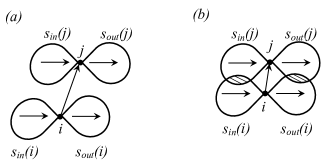
Figure 2: The addition of the edge $(i\rightarrow j)$ directed from vertex $i$ to vertex $j$ increases the out-component $s_{out}(i)$ of $i$ by an amount $s_{out}(j)$ and also increases the in-component $s_{in}(j)$ of $j$ by an amount $s_{in}(i)$. (a) In- and out-components of $i$ and $j$ do not intersect each other. (b) There are intersections between the in-and out-components.

Let us choose at random two vertices $i$ and $j$ and add a directed edge $(i\rightarrow j)$ from $i$ to $j$ (see Fig. 2). If $j$ does not belong to the out-component of $i$, or $i$ does not belong to the in-component of $j$, then this edge increases the out-component of vertex $i$ and the in-component of vertex $j$ by values

$$\Delta s_{out}(i) {=} 1{+}s_{out}(j){-}N(s_{out}(i)\cap s_{out}(j)),$$

$$\Delta s_{in}(j) {=} 1{+}s_{in}(i){-}N(s_{in}(i)\cap s_{in}(j)),$$ (27)

respectively. Here the number of vertices lying in the intersections of the out- and in-components of vertices $i$ and $j$ is subtracted,

$$N(s_{out}(i)\cap s_{out}(j)) = \sum_{k}C(j\rightarrow k)C(i\rightarrow k),$$

$$N(s_{in}(i)\cap s_{in}(j)) = \sum_{k}C(k\rightarrow i)C(k\rightarrow j).$$ (28)

The mean values of $\Delta s_{out}(i)$ and $\Delta s_{in}(j)$, averaged over pairs of vertices $i$ and $j$, are

$$\langle\Delta s_{out}\rangle {=} \frac{1}{N^{2}}\sum_{i,j\in\mathcal{G}}\Delta s_{out}(i)$$

$${=} \frac{1}{N^{2}}\sum_{i,j,k\in\mathcal{G}}[1{-}C(i{\rightarrow}j)]C(j{\rightarrow}k)[1{-}C(i{\rightarrow}k)],$$

$$\langle\Delta s_{in}\rangle {=} \frac{1}{N^{2}}\sum_{i,j\in\mathcal{G}}\Delta s_{in}(j)$$ (29)

$${=} \frac{1}{N^{2}}\!\!\!\sum_{i,j,k\in\mathcal{G}}\!\!\![1{-}C(i{\rightarrow}j)]C(k{\rightarrow}j)[1{-}C(k{\rightarrow}i)].$$

The multiplier $1{-}C(i{\rightarrow}j)$ in these equations takes into account the fact that if $j$ belongs to the out-component of $i$ (or equivalently $i$ belongs to the in-component of $j$), then the edge addition gives no contribution to $\Delta s_{out}(i)$ and $\Delta s_{in}(j)$. Assuming that all moments of the probability distribution functions $\Pi_{in}(s)$ and $\Pi_{out}(s)$ are finite, we find that the intersections between the in- and out-components give a contribution of order $O(1/N)$ to $\langle\Delta s_{in}\rangle$ and $\langle\Delta s_{out}\rangle$. Thus, in the infinite size limit $N\rightarrow\infty$, we obtain

$$\langle\Delta s_{in}\rangle=\langle\Delta s_{out}\rangle=1{+}\langle s_{in}\rangle=1{+}\langle s_{out}\rangle=\chi_{d}$$ (30)

This equation shows that the susceptibility $\chi_{d}$ determines an increase of the individual in- and out-components of vertices due to the addition of one edge at random. The larger $\chi_{d}$ the stronger the network response to edge addition.

Let us add a bidirectional edge between a randomly chosen vertices $i$ and $j$. If $i$ does not belong to the individual total component of vertex $j$, and vice versa, then the addition of this edge increases the total size of the in- and out-components of $i$ and $j$ by values

$$\Delta s_{t}(i) {=} 1{+}s_{t}(j)-\sum_{k}C(j,k)C(i,k),$$

$$\Delta s_{t}(j) {=} 1{+}s_{t}(i)-\sum_{k}C(j,k)C(i,k).$$ (31)

Here, the intersections of the in- and out-components of $i$ and $j$ are subtracted. Assuming that all moments of the probability distribution function $\Pi_{t}(s)$ are finite in the infinite size limit $N\rightarrow\infty$, we find

$$\langle\Delta s_{t}\rangle=1+\langle s_{t}\rangle=\chi_{t}.$$ (32)

Therefore, the susceptibility $\chi_{t}$ quantifies the response to the addition of a bidirectional edge at random.

V.2 Response to edge addition above the percolation point

If a directed network $\mathcal{G}$ has nonempty $G_{S}$, $IN$, and $OUT$, then the result of the addition of new edges between two vertices depends on the properties of the network parts to which these vertices belong. The addition of edges between two vertices in $F$ is described by Eq. (29) where we must sum over pairs of vertices $(i,j)\in F$. This process leads to the response Eq. (30) determined by the susceptibility $\chi_{d}$, Eq. (17). Below we only consider some particular cases of the addition of edges in order to demonstrate that a response of the network is quantified by the susceptibilities. A detailed analysis of the impact of edge pruning on the sizes of $G_{S}$, $IN$, $OUT$, and $F$ can be performed for a directed uncorrelated random network (see Sec. VI).

V.2.1 Impact on $IN$ and $OUT$

The addition of edges between pairs of vertices $(i,j)\in IN$ or $(i,j)\in OUT$ does not change the sizes of $IN$ and $OUT$. Let us choose randomly a vertex $i\in G_{out}=OUT\cup G_{S}$ and a vertex $j$ in the finite component $F$ (tendrils, tubes, and finite disconnected clusters). We add an edge $(i\rightarrow j)$ directed from $i$ to $j$ (see Fig. 3). As a result, all vertices in the out-component $s_{out}(j)$ of $j$ become a part of $OUT$ because now there is a directed path from vertices in $G_{S}$ through $i$ to any vertex in $s_{out}(j)$. Vertices belonging the intersections between $s_{out}(j)$ and $OUT$ (the shaded regions in Fig. 3 (b)) already belong to $OUT$ and should not be considered. Thus, $OUT$ increases by the value,

$$\Delta N(OUT)=\frac{1}{N(F)}\sum_{j,k\in F}C(j\rightarrow k)=\chi_{d},$$ (33)

where we used the definition Eq. (15). Note that the edge $(j\rightarrow i)$ does not change the size of $OUT$.

In the same way, we find the response of $IN$ to the addition of an edge $(j\rightarrow i)$ directed from vertex $j\in F$ to vertex $i\in IN\cup G_{S}$ chosen at random. In this case

$$\Delta N(IN)=\frac{1}{N(F)}\sum_{j,k\in F}C(k\rightarrow j)=\chi_{d}.$$ (34)

Therefore the susceptibility $\chi_{d}$ quantifies the response of $IN$ and $OUT$ to the addition of edges between vertices in $IN$ and $OUT$ and vertices in $F$.

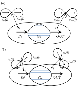
Figure 3: Addition of the edge ($i\rightarrow j$) from vertex $i\in OUT$ (or $G_{S}$) to vertex $j\in F$ and the edge ($j\rightarrow i$) from vertex $j\in F$ to vertex $i\in IN$ (or $G_{S}$). (a) There are no intersections between the in- and out-component of vertex $j\in F$ and $IN$ and $OUT$. (b) The in- and out-components of vertex $j$ intersect $IN$ and $OUT$ (the shaded regions).

V.2.2 Impact on $G_{S}$

The addition of edges between pairs of vertices $i$ and $j$ belonging to the giant strongly connected component $G_{S}$ does not change its size. Let us choose at random two vertices, one vertex $i$ in $IN$ ($i\in IN$) and the other vertex $j$ in $G_{S}$ ($j\in G_{S}$), and make a directed link ($j\rightarrow i$) from $j$ to $i$ (see Fig. 4). One can see that all vertices $l\in IN$ for which $C(i\rightarrow l)=1$ become a part of $G_{S}$ because they satisfy the criterion formulated in Sec. II, i.e., these vertices can now reach any vertex in $G_{S}$ by following edges either backwards or forwards [see Fig. 4(a)]. Thus the size $N(G_{S})$ of $G_{S}$ increases by a value $\sum_{l\in IN}C(i\rightarrow l)$. On average, this value per one added edge is

$$\Delta N(G_{S})=\frac{1}{N(IN)}\sum_{i,l\in IN}C(i\rightarrow l)=\chi_{in}^{(S)},$$ (35)

where we used Eq. (IV). Note that the addition of a directed edge ($i\rightarrow j$) does not change $G_{S}$.

Let us add a directed edge ($i\rightarrow j$) from vertex $i\in OUT$ to vertex $j\in G_{S}$. Then all vertices $l\in OUT$ for which $C(l\rightarrow i)=1$ will belong to $G_{S}$ [see Fig. 4(b)]. In this case, the size $N(G_{S})$ of $G_{S}$ increases by a value

$$\Delta N(G_{S})=\frac{1}{N(OUT)}\sum_{l\in OUT}C(l\rightarrow i)=\chi_{out}^{(S)},$$ (36)

where we used Eq. (IV). The addition of a directed edge ($j\rightarrow i$) does not change the size of $G_{S}$. One can also increase $G_{S}$ by adding an edge $(j\rightarrow i)$ directed from vertex $j\in OUT$ to vertex $i\in IN$ (see Fig. 5). On average, the addition of this edge increases the size of $G_{S}$ by the value $\chi_{in}^{(S)}+\chi_{out}^{(S)}$ per one added edge while the addition of the edge $(i\rightarrow j)$ does not change $G_{S}$. This edge is an edge-tube. Note that the addition of edges represented in Figs. 4 and 5 results in the formation new feedback loops in the modified $G_{S}$.

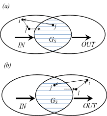
Figure 4: (Color online) (a) The addition of an edge directed from vertex $j\in G_{S}$ to vertex $i\in IN$ increases the size of the giant strongly connected component $G_{S}$ due to vertices $l\in IN$ reachable from $i$. (b) The addition of an edge directed from vertex $i\in OUT$ to vertex $j\in G_{S}$ increases $G_{S}$ due to vertices $l\in OUT$ from which $i$ can be reached.

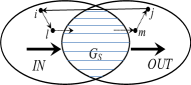
Figure 5: (Color online) The addition of an edge directed from vertex $j\in OUT$ to vertex $i\in IN$ increases the size of the giant strongly connected component $G_{S}$ at the expense of vertices $l\in IN$ reachable from $i$ and vertices $m\in OUT$ which can reach $j$ by following edge directions.

One can increase the size of the giant strongly connected component $G_{S}$ by choosing at random a vertex $j$ belonging to $F$ and connecting it by a bidirectional edge with any vertex $i\in G_{S}$. $G_{S}$ increases on average by the value

$$\Delta N(G_{S})=\frac{1}{N(F)}\sum_{j\in F}[1+s^{(F)}_{t}(j)]=\chi_{t}.$$ (37)

The susceptibilities $\chi_{in}^{(S)}$ and $\chi_{out}^{(S)}$ quantify the sensitivity of the giant strongly connected component $G_{S}$ to the addition of one edge at random. According to Eqs. (IV) and (IV), these susceptibilities are determined by the statistics of the individual finite in- and out- components of vertices in $IN$ and $OUT$, respectively. The susceptibilities are related with the probability distribution functions $\Pi_{in}^{(G)}(s)$ and $\Pi_{out}^{(G)}(s)$ of $s_{in}(IN)$ and $s_{out}(OUT)$ in $IN$ and $OUT$, respectively, similarly to Eq. (25). The susceptibilities $\chi_{in}^{(S)}$ and $\chi_{out}^{(S)}$ have no analogy in undirected networks. They exist only in the phase with the giant strongly connected component $G_{S}$. Below we will show that $\chi_{in}^{(S)}$ and $\chi_{out}^{(S)}$ diverge at the critical percolation point. This divergence is due to the divergence of $\langle s_{in}^{(IN)}\rangle$ and $\langle s_{out}^{(OUT)}\rangle$.

V.2.3 Addition of a directed edge at random

Let us add a directed edge between two randomly chosen vertices $i$ and $j$ in $\mathcal{G}$ and find how it changes sizes of $F$, $IN$, $OUT$, and $G_{S}$. The edge can be directed with the probability $1/2$ either from $i$ to $j$ or from $j$ and $i$. The processes in Figs. 3-5 give

$$\Delta N(F) = -\frac{1}{2}\chi_{d}S_{F}(S_{S}+S_{IN})-\frac{1}{2}\chi_{d}S_{F}(S_{S}+S_{OUT}),$$

$$\Delta N(IN) = \frac{1}{2}\chi_{d}S_{F}(S_{S}+S_{IN})-\frac{1}{2}\chi_{IN}^{(S)}S_{S}S_{IN}$$

$$- \frac{1}{2}[\chi_{in}^{(S)}+\chi_{out}^{(S)}]S_{OUT}S_{IN},$$

$$\Delta N(OUT) = \frac{1}{2}\chi_{d}S_{F}(S_{S}+S_{OUT})-\frac{1}{2}\chi_{OUT}^{(S)}S_{S}S_{OUT}$$

$$- \frac{1}{2}[\chi_{in}^{(S)}+\chi_{out}^{(S)}]S_{OUT}S_{IN},$$

$$\Delta N(G_{S}) = \frac{1}{2}\chi_{in}^{(S)}S_{IN}S_{S}+\frac{1}{2}\chi_{out}^{(S)}S_{OUT}S_{S}$$ (38)

$$+ \frac{1}{2}[\chi_{in}^{(S)}+\chi_{out}^{(S)}]S_{OUT}S_{IN}.$$

where $S_{F}\equiv N(F)/N$, $S_{IN}\equiv N(IN)/N$, $S_{OUT}\equiv N(OUT)/N$, and $S_{S}\equiv N(G_{S})/N$ are the fraction of vertices belonging to $F$, $IN$, $OUT$, and $G_{S}$. Therefore, at $p>p_{c}$ the addition of an edge at random decreases the size of $F$ due to the processes in Fig. 3 while the size of $G_{S}$ increases due to the processes in Figs. 4 and 5. The sizes of $IN$ and $OUT$ can both increase and decrease in dependence on the values of the negative contribution from the processes in Figs. 4 and 5 and the positive contribution from the processes in Fig. 3. One can see this behavior in Figs. 7 and 8 displaying results of our simulations for some real and synthetic directed complex networks.

VI Susceptibility of randomly damaged uncorrelated directed networks

In the previous section we introduced the susceptibility quantifying the sensitivity of different parts of directed networks to damage. In this section we find analytically the susceptibility of randomly damaged uncorrelated random directed complex networks. In this kind of complex networks, degree-degree correlations between different vertices are absent. Moreover, such complex networks have locally tree-like structure.

Let us consider the case of a randomly damaged uncorrelated directed network $\mathcal{G}$ and $p$ is the occupation probability of vertices in this network. In other wards, vertices are removed with the probability $1-p$ and remain in the network with the probability $p$. With increasing the fraction of removed vertices (this corresponds to decreasing the occupation probability $p$) the giant strongly connected component $G_{S}$ decreases while the finite directed components $F$ grow. The network undergoes the percolation phase transition at the critical point $p_{c}$ at which $G_{S}$ disappears. At $p<p_{c}$ there are only finite directed components. Structural changes caused by random removal of vertices or edges in the directed network can be described analytically by use of the generating function method Newman et al. (2001); Dorogovtsev et al. (2001); Schwartz et al. (2002); Boguñá and Serrano (2005), which gives exact results for uncorrelated random complex networks in the infinite size limit. Note that the same generating function method can be used for analyzing edge pruning. Real directed networks are correlated and have a finite size and a large clustering coefficient Fagiolo (2007); Bianconi et al. (2008). Nevertheless, we expect that even in this case one can use the results obtained by the generating function methods. These results provide a qualitatively correct though approximate description of structural changes caused by damage.

VI.1 Susceptibility $\chi_{d}$

Let us find the susceptibilities $\chi_{d}$ and $\chi_{t}$ [see Eqs. (17), (18)] of randomly damaged uncorrelated directed networks. On-site correlations between in- and out-degrees are characterized by a function $P(q_{i},q_{o})$, which is the probability that a randomly chosen vertex has in-degree $q_{i}$ and out-degree $q_{o}$. The mean in- and out-degrees are $\langle q_{i}\rangle\equiv\sum_{q_{i},q_{o}}q_{i}P(q_{i},q_{o})$ and $\langle q_{o}\rangle\equiv\sum_{q_{i},q_{o}}q_{o}P(q_{i},q_{o})$, respectively. Note that $\langle q_{i}\rangle=\langle q_{o}\rangle$ in any directed network. First we consider the case when all edges are directed and there are no bidirectional edges. The case when there are both directed and bidirectional edges will be considered in Sec. C. Due to the tree-like structure, the total size $s_{t}^{(F)}(i)$ of the in- and out-components of vertex $i\in F$ in Eq. (11) is the sum $s_{in}^{(F)}(i)+s_{out}^{(F)}(i)$ because $s_{in}^{(F)}(i)$ and $s_{out}^{(F)}(i)$ do not intersect each other. Equation (21) gives

$$\chi_{t}=2\chi_{d}-1.$$ (39)

According to Eq. (17), the susceptibility $\chi_{d}$ is determined by the mean size of the individual in- or out-components ($\langle s_{in}^{(F)}\rangle$ or $\langle s_{out}^{(F)}\rangle$) of vertices belonging to $F$. In order to find these parameters we use the generating function method described in Appendix A. Using Eqs. (66), (67), (76), and (77), we find explicitly the susceptibility $\chi_{d}$ in uncorrelated random directed complex networks at $p\leq p_{c}$,

$$\chi_{d}=1+\frac{\langle q_{o}\rangle pp_{c}}{p_{c}-p},$$ (40)

where $p_{c}=\langle q_{o}\rangle/\langle q_{i}q_{o}\rangle$, see Eq. (49). Using Eqs. (61), (62), (75), and (76) in Appendices A and B, we find $\langle s_{out}^{(F)}\rangle$ and the critical behavior of susceptibility $\chi_{d}$ above the critical point ($p>p_{c}$),

$$\chi_{d}\approx\frac{\langle q_{o}\rangle pp_{c}}{3(p-p_{c})}.$$ (41)

Thus, according to Eqs. (40) and (41), the susceptibility $\chi_{d}$ diverges as $A_{\chi}/|p-p_{c}|$ when the directed network approaches the critical percolation point $p_{c}$ both from below and above. The difference is only in the amplitude $A_{\chi}$, which is three times smaller at $p>p_{c}$ in comparison with the one at $p\leq p_{c}$, i.e.,

$$\frac{\chi_{d}(p\rightarrow p_{c}-0)}{\chi_{d}(p\rightarrow p_{c}+0)}=3$$ (42)

Our numerical simulations in Sec. VII confirm the analytical results. Note that in the framework of the phenomenological Landau theory of continuous phase transitions (see, for example, Goltsev et al. (2003)), the ratio $\chi(p\rightarrow p_{c}-0)/\chi(p\rightarrow p_{c}+0)$ is 1 for the percolation transition in contrast to 3 in Eq. (42). For comparison, $\chi(T\rightarrow T_{c}-0)/\chi(T\rightarrow T_{c}+0)=2$ for the ferromagnetic transition within the mean-field theory.

Based on Eqs. (40), (41), and (64), we conclude that in uncorrelated random directed networks the susceptibility $\chi_{d}$ and the order parameter $S_{IO}$ demonstrate the critical behavior: $\chi_{d}\propto|p-p_{c}|^{-\gamma}$ and $S_{IO}\propto(p-p_{c})^{\beta}$ with the standard critical exponents $\gamma=1$ and $\beta=1$. We find the same critical behavior in the uncorrelated random directed networks with bidirectional edges (see Appendix C).

VI.2 Susceptibilities $\chi_{in}^{(S)}$ and $\chi_{out}^{(S)}$

Let us find the susceptibilities $\chi_{in}^{(S)}$ and $\chi_{out}^{(S)}$ quantifying the sensitivity of $G_{S}$ to the addition of edges in directed random uncorrelated networks. According to Eqs. (IV) and (IV), $\chi_{in}^{(S)}$ and $\chi_{out}^{(S)}$ are determined by the mean size of the individual in- and out-components, $\langle s_{in}^{(IN)}\rangle$ and $\langle s_{out}^{(OUT)}\rangle$ of vertices in $IN$ and $OUT$, respectively. Using Eqs. (61), (62), and (68), in the leading order of $(p-p_{c})/p_{c}$ at $p>p_{c}$, we find the critical behavior

$$\chi_{in}^{(S)}{\approx}\chi_{out}^{(S)}{\approx}\frac{\langle q_{i}q_{o}\rangle}{\langle q_{i}\rangle}\frac{p_{c}^{2}}{p-p_{c}},$$ (43)

(see Eqs. (78) and (79)). Using Eqs. (41) and (43), at $p$ near $p_{c}$ we find the ratio

$$\frac{\chi_{in}^{(S)}}{\chi_{d}}=\frac{3\langle q_{i}q_{o}\rangle}{\langle q_{i}\rangle\langle q_{o}\rangle}.$$ (44)

In Sec. VII we analyze numerically the critical behavior of $\chi_{in}^{(S)}$ and $\chi_{out}^{(S)}$ in real and synthetic directed networks.

VI.3 Statistics of the in- and out-components of vertices

In the case of uncorrelated random complex networks, the distribution functions $\Pi_{in}^{(F)}(s)$ and $\Pi_{out}^{(F)}(s)$ [see Eq. (24)] are related with the generating functions Eqs. (70) and (71) in Appendix B. Using the analytical method developed in Newman et al. (2001), we find that these distribution functions have the following asymptotic behavior:

$$\Pi_{out}^{(F)}(s)\propto Y_{in}^{(F)}(s)\propto\frac{1}{s^{3/2}}e^{-s/s^{*}}$$ (45)

both below and above $p_{c}$. The parameter $s^{*}$ behaves as $s^{*}\propto(p-p_{c})^{-2}$. At $p$ below $p_{c}$ the asymptotic behavior Eq. (45) was found in Schwartz et al. (2002). The distribution functions $\Pi_{in}^{(F)}(s)$ and $\Pi_{out}^{(F)}(s)$ have the power-law behavior $s^{-3/2}$ at the critical point $p_{c}$. We find the same asymptotic behavior Eq. (45) for the probability distribution functions $\Pi_{in}^{(IN)}(s)$ and $\Pi_{out}^{(OUT)}(s)$ of the in-component $s_{in}^{(IN)}(i)$ and the out-component $s_{out}^{(OUT)}(i)$ of vertices $i\in OUT$ and $i\in OUT$, respectively.

VII Susceptibility of real and synthetic directed networks

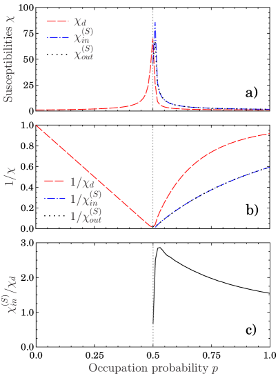
Figure 6: (Color online). (a) Susceptibilities $\chi_{d}$, $\chi_{in}^{(S)}$, and $\chi_{out}^{(S)}$ versus the occupation probability $p$ in an Erdős-Rényi network of size $N=10^{6}$ and the mean in- and out degrees $\langle q_{i}\rangle=\langle q_{o}\rangle=2$. (b) Reciprocal susceptibilities: $1/\chi_{d}$, $1/\chi_{in}^{(S)}$, and $1/\chi_{out}^{(S)}$ versus $p$. (c) The ratio $\chi_{in}^{(S)}/\chi_{d}$ above $p_{c}$. 100 network realizations were used for each value of p, and in each realization $10\%$ of the vertices were sampled randomly.

In this section we discuss the results of our numerical simulations of the susceptibilities $\chi_{d}$, $\chi^{(S)}_{in}$ , and $\chi^{(S)}_{out}$ in randomly damaged real and synthetic networks. In Sec. IV we showed that these susceptibilities are determined by the two-point connectivity function $C(i\rightarrow j)$ [see Eqs. (15), (IV) and (IV)]. Unfortunately, it is computationally inefficient to explicitly find $C(i\rightarrow j)$. An alternative numerical method for finding these susceptibilities is to use the fact that, according to Eqs. (17), (IV) and (IV), the susceptibilities are determined by the mean size of the finite individual in- and out- components of vertices in the network parts $F$, $IN$, and $OUT$ (see Fig. 1). Thus, the statistical analysis of the individual in- and out-components of randomly chosen vertices allows us to find numerically the susceptibilities both above and below the percolation transition. In the simulations, the networks under consideration were randomly damaged, i.e., edges were removed with a probability $1{-}p$ and were retained with an occupation probability $p$. We found $F$, $IN$, $OUT$, and $G_{S}$ of the damaged networks. Note that since the networks studied in the simulations have a finite size, we considered the largest strongly connected component as $G_{S}$. Then we chose a sample subset of vertices uniformly at random from $F$, $IN$, and $OUT$, and determined the sizes of the individual in- and out components of vertices in these components [see Eqs. (9)-(12), (IV) and (IV)]. These sizes were averaged over the vertices in the chosen subset, and over many realizations of the damage, to arrive at estimates for the susceptibilities [see Eqs. (17), (IV) and (IV)]. Figure 6 represents results of our simulations for the Erdős-Rényi networks with uncorrelated in- and out-degrees. The susceptibilities $\chi_{d}$, $\chi^{(S)}_{in}$, and $\chi^{(S)}_{out}$ demonstrate a sharp maximum that signals the percolation transition. Equation (49) predicts that the critical point of the Erdős-Rényi network is $p_{c}=\langle q_{i}\rangle/\langle q_{i}q_{o}\rangle=1/\langle q_{i}\rangle$. In the simulations we studied networks with the mean in- and out degrees $\langle q_{i}\rangle=\langle q_{o}\rangle=2$, i.e., $p_{c}=0.5$. In this case, equation (40) gives $1/\chi_{d}=(p_{c}-p)/p_{c}=1-2p$ in the region $0\leq p\leq p_{c}$ where there are only finite directed components and disconnected clusters. This theoretical prediction is in complete agreement with our simulations in Fig. 6(b) (see the red dashed line at $0\leq p\leq 0.5$). The critical behavior of $\chi^{(S)}_{in}$ and $\chi^{(S)}_{out}$ is shown in Fig. 6(a) and 6(b). Studying networks of different size $N$, we observed that the maxima of $\chi_{d}$, $\chi^{(S)}_{in}$, and $\chi^{(S)}_{out}$ increase with increasing $N$ showing the tendency for the divergence in the limit $N\rightarrow\infty$. Results in Fig. 6(b) also show that the susceptibility $\chi_{d}$ has different slopes at $p$ above and below $p_{c}$, in agreement with Eqs. (41) and (42), which predict $p_{c}/[(p_{c}-p)\chi_{d}]=1$ at $p\leq p_{c}$ and $p_{c}/[(p-p_{c})\chi_{d}]=3$ at $p>p_{c}$. At $p>p_{c}$ the reciprocal susceptibilities $\chi^{(S)}_{in}$ and $\chi^{(S)}_{out}$ behave as follows: $1/\chi^{(S)}_{in}=1/\chi^{(S)}_{out}\approx(p-p_{c})/p_{c}=2p-1$ in agreement with Eq. (43) [see the blue dot-dashed line in Fig. 6(b)]. Figure 6(c) displays the ratio $\chi^{(S)}_{in}/\chi_{d}$. One can see that this ratio tends to 3 at $p\rightarrow p_{c}$ in agreement with Eq. (44). $\chi^{(S)}_{in}$ achieves a maximum at $p_{max}$ slightly above $p_{c}$. This shift of $p_{max}$ from $p_{c}$ is due to a finite-size effect. It becomes smaller and smaller with increasing $N$.

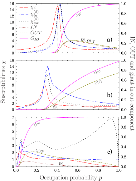
Figure 7: (Color online) Susceptibilities $\chi_{d}$, $\chi^{(S)}_{in}$, and $\chi^{(S)}_{out}$, and the relative sizes of $IN$, $OUT$ and $G_{IO}$ versus the occupation probability $p$: (a) an Erdős-Rényi network of size $N=10^{4}$; (b) the Gnutella p2p file sharing network ($N=62586,\langle q_{tot}\rangle=4.726$ kon (2016a); Ripeanu et al. (2002)); (c) the neural network of C. elegans ($N=495,\langle q_{tot}\rangle=32.073$ Jarrell et al. (2012)). The vertical dashed lines correspond to $p_{c}$ determined by the message passing method of Timár et al. (2017).

We found a similar critical behavior of the susceptibilities in the Gnutella p2p filesharing network kon (2016a); Ripeanu et al. (2002) and the neural network of C. elegans Jarrell et al. (2012) (see Fig. 7 where an Erdős-Rényi network is also displayed for comparison). Our analysis of data Jarrell et al. (2012) showed that that the main body of the male C. elegans consists of 495 vertices wired by both chemical and electrical synapses. There are 492 nodes in the $G_{S}$, 1 node in $IN$ and 2 nodes in $OUT$. In Fig. 7 we show the behavior of the relative sizes of $IN$, $OUT$, and the order parameter $G_{IO}$, which is the union $G_{IO}=G_{S}\cup IN\cup OUT$ [Eq. (5)], as functions of the occupation probability $p$. The maximum of $\chi_{d}$ signals the percolation transition. The position of the maximum agrees very well with $p_{c}$ predicted by the message passing algorithm of [19]. Notice that the maxima of the susceptibilities $\chi^{(S)}_{in}$ and $\chi^{(S)}_{out}$ are slightly shifted, compared to the maximum of $\chi_{d}$. This shift is due to a finite size effect similar to the one in the Erdős-Rényi network in Fig. 6 (a). In the Erdős-Rényi network, the sizes of $IN$ and $OUT$ achieve a maximum and then decrease with increasing $p$, in contrast to the strictly monotonic increase of $G_{IO}$. This feature is shared by the C. elegans network. However the size of $OUT$ in the Gnutella network increases monotonically, without producing a maximum. The susceptibilities $\chi_{d}$, $\chi^{(S)}_{in}$, and $\chi^{(S)}_{out}$ of the Gnutella network, after their peak at $p_{c}$ decrease monotonically, similarly to their behavior in the Erdős-Rényi network. A striking exception from this rule is the susceptibility $\chi^{(S)}_{out}$ in the C. elegans network, which exhibits a strongly non-monotonic behavior [two additional broad maxima above $p_{c}$, apart from the sharp maximum at $p_{c}\approx 0.04$ in Fig. 7 (c), dotted line]. This unusual behavior is due to the structural peculiarities of the C. elegans network. We suggest that the maximum at $p\approx 0.92$ is due to the chains of bodywall muscle neurons, which all have exactly $2$ outgoing connections (to their neighbors on either side), and multiple in-coming ones. Pruning of some connections between these neurons in the chain increases significantly the $OUT$ and, in turn, increases $\chi^{(S)}_{out}$ even at small damage. The origin of the maximum at the intermediate $p$ ($p\approx 0.2$), is unclear and needs a more detailed analysis of the impact of pruning on the C. elegans network.

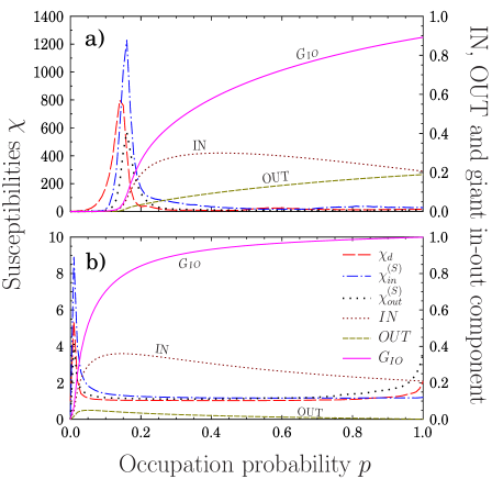
Figure 8: (Color online). Susceptibilities $\chi_{d}$, $\chi^{(S)}_{in}$, and $\chi^{(S)}_{out}$, and the relative sizes of $IN$, $OUT$ and $G_{IO}$ versus the occupation probability $p$: (a) a sample of the World Wide Web ($N=875713,\langle q_{in}\rangle=5.83$ kon (2016b); Leskovec et al. (2008)), (b) a sample of Twitter ($N=456631,\langle q_{in}\rangle=32.53$ Kwak et al. (2010)).

In Figs. 8 (a) and (b) we present results of our simulations for samples of two well-known, inherently directed networks, the World Wide Web kon (2016b); Leskovec et al. (2008) and Twitter Kwak et al. (2010). Note that in the WWW a directed link from $i$ to $j$ means that there is a hyperlink from site $i$ pointing to site $j$. In Twitter, a directed link from $i$ to $j$ means that $i$ follows $j$. Both networks have similar wide in-degree distributions, rapidly decaying out-degree distributions, and similar sizes. In both networks, $IN$ is larger than $OUT$. This is especially apparent in Twitter. An interesting observation is that the susceptibilities in the WWW are, especially near their maximum, much higher than those of Twitter. The difference is a striking two orders of magnitude! We suggest that such high susceptibilities in the WWW are due to the highly modular structure of the network. This modular structure results in very large sizes of the in- and out-components of vertices either in $IN$, $OUT$ or $F$ in the undamaged samples of the WWW network. More specifically, the undamaged WWW has $12874$ nontrivial strongly connected components (SCCs), i.e., ones of size at least 2. There are $19$ SCCs with sizes greater than $100$. The size of the second largest SCC is $968$. The mean size of SCCs, excluding the giant (largest) SCC, is $6.37$. In contrast, the Twitter sample has only $3854$ nontrivial SCCs, none of which are larger than $100$ vertices. The second largest SCC has only $17$ vertices. The mean size of SCCs , excluding the giant (largest) SCC, is $2.23$. The susceptibilities $\chi_{d}$ and $\chi_{out}^{(S)}$ of the Twitter network in Fig. 8 (b) demonstrate non-monotonous behavior as a function of $p$ similar to the one in the C. elegans network. Apart from the peak at $p_{c}$ there is a peak at $p=1$ in contrast to $\chi_{in}^{(S)}$, which decreases monotonously at $p>p_{c}$. The origin of this behavior is unclear. Further investigations are required to explain our numerical findings in detail, but based on the results presented above one can see how a simple and straightforward analysis of the susceptibility of directed networks can reveal their structural peculiarities, such as those found in the C. elegans, WWW, and Twitter.

VIII Conclusion

In this paper, we studied the sensitivity of directed networks with both directed and bidirectional edges to the addition and pruning of edges and vertices. We demonstrated that different network parts [the giant strongly connected component $G_{S}$, which is a central core of the network, the sets $IN$ and $OUT$ playing the role of the incoming and outgoing terminals for $G_{S}$, and the finite components $F$ including tendrils, tubes, and disconnected finite clusters (see Fig. 1)] have different sensitivities to the addition and pruning of edges and vertices since these parts have different topological properties. It is not surprising that the sensitivities of the network parts to the addition and pruning of edges and vertices are quantified by different susceptibilities. We introduced the susceptibilities, using a relation between the percolation problem and the Potts model. For this purpose we introduced the two-point connectivity function, which characterizes whether any two vertices are connected by a directed path or not. This two-point connectivity function allowed us to find explicitly the susceptibilities of the network parts. Since it is computationally inefficient to find this function in a large network, we also proposed an alternative method for finding the susceptibilities. Our method is based on the fact that, according to Eqs. (17), (IV) and (IV), the susceptibilities are determined explicitly by the mean size of the finite individual in- and out- components of vertices in the corresponding network parts, i.e., $IN$, $OUT$, and $F$. We found analytically the susceptibilities in directed uncorrelated random networks by use of the generating function method. We showed that the susceptibilities diverge at the critical point of the directed percolation transition, signaling the appearance (or disappearance) of the giant strongly connected component in the infinite size limit. In finite networks due to the finite size effect, the susceptibilities demonstrate a sharp peak at the percolation point. We performed numerically the statistical analysis of the individual in- and out-components of vertices and found the susceptibilities of randomly damaged real and synthetic directed complex networks, such as the World Wide Web, Twitter, the neural network of Caenorhabditis elegans, the Gnutella p2p filesharing network, and directed Erdős-Rényi graphs. Our analysis revealed a non-monotonous dependence of the sensitivity of $OUT$ to random pruning of edges or vertices in Caenorhabditis elegans and Twitter. This behavior manifests specific structural peculiarities of these networks. Our preliminary analysis pointed out the possible role of chain-like motives in the observed effects. Comparing the susceptibility of $OUT$ in the WWW and Twitter we made the interesting observation that the former, especially near their maximum, is two orders of magnitude higher than the latter. We suggest that such high susceptibility of the WWW is due to the modular structure of the network. Further investigations are necessary to explain our numerical findings in detail. We believe that measurements of the sensitivity of different parts of directed networks to the addition or pruning of edges and vertices can be an effective method for studying structural peculiarities of the networks.

IX Acknowledgements

This work was supported by the grant PEST UID/CTM/50025/2013.

Appendix A Generating function technique

Let us consider directed uncorrelated random complex networks. On-site correlations between in- and out-degrees are characterized by a function $P(q_{i},q_{o})$, which is the probability that a randomly chosen vertex has in-degree $q_{i}$ and out-degree $q_{o}$. These complex network have locally tree-like structure that enables us to use the generating function technique Newman et al. (2001); Dorogovtsev et al. (2001) in order to find the size of the giant strongly connected component and statistics of finite directed components. We consider the case of a randomly damaged network and $p$ is the occupation probability of vertices in the considered network.

Let us first consider the following process in a graph $\mathcal{G}$. Choose at random an edge and move along this edge forwards. We define $Y_{out}(s)$ as the probability to reach $s$ vertices by following edges forwards. We also define the probability $Y_{in}(s)$ to reach $s$ vertices by following edges backwards. We introduce generating functions,

$$H_{out}(x) = \sum_{s=0}^{\infty}x^{s}Y_{out}(s),$$

$$H_{in}(x) = \sum_{s=0}^{\infty}x^{s}Y_{in}(s),$$ (46)

which are determined by the following self-consistency equations Newman et al. (2001); Dorogovtsev et al. (2001):

$$H_{out}(x) {=} 1{-}p{+}\frac{px}{\langle q_{i}\rangle}\sum_{q_{i},q_{o}}q_{i}P(q_{i},q_{o})[H_{out}(x)]^{q_{o}},$$ (47)

$$H_{in}(x) {=} 1{-}p{+}\frac{px}{\langle q_{o}\rangle}\sum_{q_{i},q_{o}}q_{o}P(q_{i},q_{o})[H_{in}(x)]^{q_{i}}.$$ (48)

There is a critical point

$$p_{c}=\frac{\langle q_{o}\rangle}{\langle q_{i}q_{o}\rangle}$$ (49)

below which, i.e., at $p<p_{c}$, equations (47) and (48) have the only one solution corresponding to $H_{in}(1)=H_{out}(1)=1$. At $p>p_{c}$, another solution corresponding to $H_{in}(1)\equiv x_{c}<1$ and $H_{out}(1)\equiv y_{c}<1$ appears. $y_{c}$ is the probability that choosing an edge at random and moving along its direction we will reach a finite number of vertices while $x_{c}$ is the probability that choosing an edge at random and moving against its direction we will reach a finite number of vertices.

The total number of remaining vertices in the damaged network is $Np$. Let us define parameters $S_{S}$, $S_{IN}$, $S_{OUT}$, and $S_{F}$ as the probabilities that a vertex chosen at random among the remaining $Np$ vertices belongs to $G_{S}$, $IN$, $OUT$, and $F$, respectively. The sizes of $G_{S}$, $IN$, $OUT$, and $F$ are $NpS_{S}$, $NpS_{IN}$, $NpS_{OUT}$, and $NpS_{F}$, respectively. In turn, the fraction $S_{S}$ of vertices belonging to $G_{S}$ ($S_{S}=N(G_{S})/Np$) is the probability that a randomly chosen vertex has at least one in-coming edge from $G_{S}$ and at least one outgoing edge leading to $G_{S}$. Using this relation, we find

$$S_{S}=\sum_{q_{i},q_{o}}(1-x_{c}^{q_{i}})(1-y_{c}^{q_{o}})P(q_{i},q_{o}).$$ (50)

The fraction $S_{IN}$ of vertices belonging $IN$ is the probability that a randomly chosen vertex has no in-coming edge from $G_{S}$ but at least one outgoing edge leading to $G_{S}$:

$$S_{IN}=\sum_{q_{i},q_{o}}x_{c}^{q_{i}}(1-y_{c}^{q_{o}})P(q_{i},q_{o}).$$ (51)

The fraction $S_{OUT}$ is the probability that a randomly chosen vertex has at least one incoming edge from $G_{S}$ but no outgoing edge leading to $G_{S}$

$$S_{OUT}=\sum_{q_{i},q_{o}}(1-x_{c}^{q_{i}})y_{c}^{q_{o}}P(q_{i},q_{o}).$$ (52)

The fraction $S_{F}$ of vertices belonging to $F$ is the probability that a vertex chosen at random has no incoming and no outgoing edges coming from or leading to $G_{S}$,

$$S_{F}=\sum_{q_{i},q_{o}}x_{c}^{q_{i}}y_{c}^{q_{o}}P(q_{i},q_{o}).$$ (53)

Introducing a generating function

$$\Phi(x,y)\equiv\sum_{q_{i},q_{o}}x^{q_{i}}y^{q_{o}}P(q_{i},q_{o}),$$ (54)

we can write the fractions of vertices in $G_{S}$, $IN$, $OUT$, $F$, and $G_{IO}$ in the following form,

$$S_{S} = 1-\Phi(x_{c},1)-\Phi(1,y_{c})+\Phi(x_{c},y_{c}),$$ (55)

$$S_{IN} = \Phi(x_{c},1)-\Phi(x_{c},y_{c}),$$ (56)

$$S_{OUT} = \Phi(1,y_{c})-\Phi(x_{c},y_{c}),$$ (57)

$$S_{F} = \Phi(x_{c},y_{c}),$$ (58)

$$S_{IO} = S_{S}+S_{IN}+S_{OUT}=1-S_{F},$$ (59)

$$1 = S_{S}+S_{IN}+S_{OUT}+S_{F},$$ (60)

Solving Eqs. (47) at $0<p-p_{c}\ll p_{c}$ in the leading order in $(p-p_{c})/p_{c}$, we find

$$x_{c}\approx 1-\frac{2\langle q_{o}\rangle(p-p_{c})}{p_{c}^{2}\langle q_{o}q_{i}(q_{i}-1)\rangle},$$ (61)

$$y_{c}\approx 1-\frac{2\langle q_{i}\rangle(p-p_{c})}{p_{c}^{2}\langle q_{o}q_{i}(q_{o}-1)\rangle}.$$ (62)

Substituting this result into Eqs. (55)–(59) gives the critical behavior

$$S_{S}\propto\Bigl{(}\frac{p-p_{c}}{p_{c}}\Bigr{)}^{2},$$ (63)

$$S_{IO},S_{IN},S_{OUT}\propto\frac{p-p_{c}}{p_{c}},$$ (64)

$$S_{F}\approx 1-O\Bigl{(}\frac{p-p_{c}}{p_{c}}\Bigr{)}.$$ (65)

The derivatives $dH_{out}(x)/dx|_{x=1}$ and $dH_{in}(x)/dx|_{x=1}$ can be found from Eqs. (47) and (48):

$$\frac{dH_{out}(x)}{dx}\Big{|}_{x=1}=\frac{\frac{p}{\langle q_{i}\rangle}\sum_{q_{i},q_{o}}q_{i}P(q_{i},q_{o})y^{q_{o}}_{c}}{1-\frac{p}{\langle q_{i}\rangle}\sum_{q_{i},q_{o}}q_{i}q_{o}P(q_{i},q_{o})y^{q_{o}-1}_{c}},$$

$$\frac{dH_{in}(x)}{dx}\Big{|}_{x=1}=\frac{\frac{p}{\langle q_{o}\rangle}\sum_{q_{i},q_{o}}q_{o}P(q_{i},q_{o})x^{q_{i}}_{c}}{1-\frac{p}{\langle q_{o}\rangle}\sum_{q_{i},q_{o}}q_{i}q_{o}P(q_{i},q_{o})x^{q_{i}-1}_{c}}.$$

(66)

These derivatives are positive both below and above $p_{c}$. They diverge at the critical point $p=p_{c}$. At $p<p_{c}$ we find the explicit result for the derivatives Eq. (66):

$$\frac{dH_{out}(x)}{dx}\Big{|}_{x=1}=\frac{dH_{in}(x)}{dx}\Big{|}_{x=1}=\frac{pp_{c}}{p_{c}-p}$$ (67)

At $p>p_{c}$, substituting Eqs. (61) and (62) into Eq. (66), we obtain the following critical behavior in the leading order in $(p-p_{c})/p_{c}\ll 1$:

$$\frac{dH_{out}(x)}{dx}\Big{|}_{x=1}\approx\frac{dH_{in}(x)}{dx}\Big{|}_{x=1}\approx\frac{pp_{c}}{p-p_{c}}$$ (68)

Appendix B Generating functions for finite components above $p_{c}$

The generating functions $H_{out}(x)$ and $H_{in}(x)$, Eqs. (47) and (48), do not allow us to find statistics of individual finite in- and out-components of vertices in the finite component $F$ above the percolation threshold. For this purpose we introduce other generating functions as follows. Choose at random an edge and move along this edge forwards. We define $Y_{out}^{(F)}(s)$ as the probability to reach $s$ vertices, which have no incoming edges by which one can reach $G_{S}$, moving backwards. Then, choose at random an edge and move backwards. We define $Y_{in}^{(F)}(s)$ as the probability to reach $s$ vertices (moving backwards), which have no outgoing edges by which one can reach $G_{S}$, moving forwards. These probabilities determine the following generating functions:

$$\widetilde{H}_{out}(x) = \sum_{s=0}^{\infty}x^{s}Y_{out}^{(F)}(s),$$

$$\widetilde{H}_{in}(x) = \sum_{s=0}^{\infty}x^{s}Y_{in}^{(F)}(s).$$ (69)

Note that $\widetilde{H}_{in}(1)$ and $\widetilde{H}_{out}(1)$ are the probabilities to reach a finite number of vertices, which have no outgoing or incoming edges from $G_{S}$, when we go against or along the edge directions, respectively. We find that in uncorrelated random directed complex networks, the generating functions $\widetilde{H}_{out}(x)$ and $\widetilde{H}_{in}(x)$ are determined by the following self-consistency equations:

$$\widetilde{H}_{out}(x) = 1{-}p{+}p\sum_{q_{i},q_{o}}\frac{q_{i}}{\langle q_{i}\rangle}(1-x_{c}^{q_{i}-1})P(q_{i},q_{o})y_{c}^{q_{o}}+$$ (70)

$$px\sum_{q_{i},q_{o}}\frac{q_{i}}{\langle q_{i}\rangle}x_{c}^{q_{i}-1}P(q_{i},q_{o})[\widetilde{H}_{out}(x)]^{q_{o}},$$

$$\widetilde{H}_{in}(x) = 1{-}p{+}p\sum_{q_{i},q_{o}}x_{c}^{q_{i}}P(q_{i},q_{o})\frac{q_{o}}{\langle q_{o}\rangle}(1-y_{c}^{q_{o}-1})+$$ (71)

$$px\sum_{q_{i},q_{o}}[\widetilde{H}_{in}(x)]^{q_{i}}P(q_{i},q_{o})\frac{q_{o}}{\langle q_{o}\rangle}y_{c}^{q_{o}-1},$$

where the parameter $x_{c}$ and $y_{c}$ are determined by Eqs. (47) and (48). The first term $1-p$ in Eqs. (70) and (71) is the probability that a vertex at the end of an edge, along which we move, is removed. The second term is the probability that a vertex at the end of an edge, along which we move, has at least one incoming edge by which one can reach $G_{S}$, moving backwards among $q_{i}-1$ incoming edges (note that one more incoming edge is the edge along which we arrive at this vertex). The second term in Eq. (71) is the probability that a vertex at the end of an edge, along which we arrived moving backwards, has at least one outgoing edge by which one can reach $G_{S}$, moving forwards among $q_{o}-1$ outgoing edges (note that one more outgoing edge is the edge along which we arrived moving backwards). At $x=1$ we have a solution $\widetilde{H}_{out}(1)=y_{c}$ and $\widetilde{H}_{in}(1)=x_{c}$. At $p<p_{c}$, we have $x_{c}=y_{c}=1$ and Eqs. (70) and (71) are reduced to Eqs. (47) and (48). It is easy to show that the probabilities $Y_{out}^{(F)}(s)$ and $Y_{in}^{(F)}(s)$ defined above, are related with the solution of Eqs. (70) and (71) as follows:

$$\frac{d^{s}\widetilde{H}_{out}(x)}{s!d^{s}x}\Big{|}_{x=0}=Y_{out}^{(F)}(s),$$

$$\frac{d^{s}\widetilde{H}_{in}(x)}{s!d^{s}x}\Big{|}_{x=0}=Y_{in}^{(F)}(s).$$ (72)

The first derivatives of $\widetilde{H}_{out}(x)$ and $\widetilde{H}_{in}(x)$ at $x=1$,

$$d\widetilde{H}_{out}(x)/dx|_{x=1}=\sum_{s=0}^{\infty}sY_{out}^{(F)}(s),$$

$$d\widetilde{H}_{in}(x)/dx|_{x=1}=\sum_{s=0}^{\infty}sY_{in}^{(F)}(s),$$ (73)

give the mean number of vertices, which are reachable by following edges either forwards or backwards and which have either no incoming or no outgoing edges with $G_{S}$, respectively. Differentiating Eqs. (70) and (71) with respect to $x$, we find

$$\frac{d\widetilde{H}_{out}(x)}{dx}\Big{|}_{x{=}1} {=} \frac{\frac{p}{\langle q_{i}\rangle}\sum_{q_{i},q_{o}}q_{i}P(q_{i},q_{o})x^{q_{i}-1}_{c}y^{q_{o}}_{c}}{1{-}\frac{p}{\langle q_{i}\rangle}\sum_{q_{i},q_{o}}q_{i}q_{o}P(q_{i},q_{o})x^{q_{i}-1}_{c}y^{q_{o}-1}_{c}},$$

$$\frac{d\widetilde{H}_{in}(x)}{dx}\Big{|}_{x{=}1} {=} \frac{\frac{p}{\langle q_{o}\rangle}\sum_{q_{i},q_{o}}q_{o}P(q_{i},q_{o})x^{q_{i}}_{c}y^{q_{o}-1}_{c}}{1{-}\frac{p}{\langle q_{o}\rangle}\sum_{q_{i},q_{o}}q_{i}q_{o}P(q_{i},q_{o})x^{q_{i}-1}_{c}y^{q_{o}-1}_{c}}.$$

Using Eqs. (61) and (62), we find that these derivatives diverge when $p$ tends to $p_{c}$ from above:

$$\frac{d\widetilde{H}_{out}(x)}{dx}\Big{|}_{x=1}\approx\frac{d\widetilde{H}_{in}(x)}{dx}\Big{|}_{x=1}\approx\frac{pp_{c}}{3(p-p_{c})},$$ (75)

The individual in- and out-components of vertex in $F$ are the sum of the number of vertices reachable by following $q_{i}$ and $q_{o}$ edges backwards or forwards, respectively, but intersections with $IN$ and $OUT$ must be excluded [see Eq. (19)]. The mean values of the individual in- and out-components can be found by use of the functions $\widetilde{H}_{out}(x)$, $\widetilde{H}_{out}(x)$, and $\Phi(x,y)$,

$$\langle s_{out}^{(F)}\rangle {=} \frac{d\Phi(x_{c},\widetilde{H}_{out}(x))}{S_{F}dx}\Big{|}_{x=1}$$ (76)

$${=} \sum_{q_{i},q_{o}}P(q_{i},q_{o})q_{o}x^{q_{i}}_{c}y^{q_{o}{-}1}_{c}\frac{d\widetilde{H}_{out}(x)}{S_{F}dx}\Big{|}_{x=1},$$

$$\langle s_{in}^{(F)}\rangle {=} \frac{d\Phi(\widetilde{H}_{in}(x)),y_{c})}{S_{F}dx}\Big{|}_{x=1}$$ (77)

$${=} \sum_{q_{i},q_{o}}P(q_{i},q_{o})q_{i}x^{q_{i}{-}1}_{c}y^{q_{o}}_{c}\frac{d\widetilde{H}_{in}(x)}{S_{F}dx}\Big{|}_{x=1}.$$

Here the derivatives are given by Eq. (LABEL:eq:_A19). At $p<p_{c}$ we have $x_{c}=y_{c}=1$ and $S_{F}=1$ since $F=\mathcal{G}$.

The mean size of the individual in-component of vertices belonging to $IN$ and the mean size of the individual out-component of vertices belonging to $OUT$ can be found by use of the generating functions $H_{in}(x)$ and $H_{out}(x)$ [see Eqs. (47) and (48)], respectively. We replace $x_{c}$ to $H_{in}(x)$ in Eq. (56) and $y_{c}$ to $H_{out}(x)$ in (57). Differentiating the obtained functions with respect to $x$, we find

$$\!\!\!\!\!\!\!\!\!\!\!\!\!\!\!\!\!\!\!\langle s_{out}^{(OUT)}\rangle {=} \frac{d[\Phi(1,H_{out}(x)){-}\Phi(x_{c},H_{out}(x))]}{S_{OUT}dx}\Big{|}_{x{=}1},$$ (78)

$$\langle s_{in}^{(IN)}\rangle {=} \frac{d[\Phi(H_{in}(x),1){-}\Phi(H_{in}(x),y_{c})]}{S_{IN}dx}\Big{|}_{x{=}1}.$$ (79)

Appendix C Susceptibility of networks with directed and bidirectional edges below $p_{c}$

The percolation transition in random complex networks with directed and bidirectional edges was studied in Boguñá and Serrano (2005). These networks are described by the probability $P(q_{i},q_{o},q_{b})$ that a vertex has $q_{i}$ incoming edges, $q_{o}$ outgoing edges, and $q_{o}$ bidirectional edges. This joint degree distribution must satisfy the condition $\langle q_{i}\rangle=\langle q_{o}\rangle$. In this section we use the generating function technique to find the susceptibilities $\chi_{d}$ and $\chi_{t}$ [Eqs. (17) and (18)] in uncorrelated random directed networks with directed and bidirectional edges.

Let us consider randomly damaged network and $p$ is the occupation probability. We will only consider the case $p<p_{c}$ for simplicity. At $p<p_{c}$ we introduce three generating functions $H_{in}(x)$, $H_{out}(x)$, and $H_{b}(x)$. They are determined by the following equations:

$$H_{out}(x) = 1{-}p{+}\frac{px}{\langle q_{i}\rangle}\sum_{q_{i},q_{o},q_{b}}q_{i}P(q_{i},q_{o},q_{b})\times$$

$$[H_{out}(x)]^{q_{o}}[H_{b}(x)]^{q_{b}},$$

$$H_{in}(x) = 1{-}p{+}\frac{px}{\langle q_{o}\rangle}\sum_{q_{i},q_{o},q_{b}}q_{o}P(q_{i},q_{o},q_{b})\times$$

$$[H_{in}(x)]^{q_{i}}[H_{b}(x)]^{q_{b}},$$

$$H_{b}(x) = 1{-}p{+}\frac{px}{\langle q_{b}\rangle}\sum_{q_{i},q_{o},q_{b}}q_{b}P(q_{i},q_{o},q_{b})\times$$ (80)

$$[H_{out}(x)]^{q_{o}}[H_{b}(x)]^{q_{b}-1},$$

These equations have a solution with $H_{in}(1)=H_{out}(1)=H_{b}(1)=1$ at $p<p_{c}$. A solution with $H_{in}(1),H_{out}(1),H_{b}(1)<1$ appears at $p>p_{c}$. The critical point $p_{c}$ is given by a quadratic equation:

$$0 {=} p_{c}^{2}\Bigr{[}\langle q_{i}q_{o}\rangle\langle q_{b}(q_{b}{-}1)\rangle{-}\langle q_{i}q_{b}\rangle\langle q_{o}q_{b}\rangle\Bigl{]}{-}$$ (81)

$$p_{c}\Bigr{[}\langle q_{i}q_{o}\rangle\langle q_{b}\rangle{+}\langle q_{b}(q_{b}{-}1)\rangle\langle q_{i}\rangle\Bigl{]}{+}\langle q_{i}\rangle\langle q_{b}\rangle.$$

The first derivatives of the functions $H_{in}(x)$, $H_{out}(x)$, and $H_{b}(x)$ at $x=1$ diverge at the critical point $p=p_{c}$:

$$\frac{dH_{out}(x)}{dx}\Big{|}_{x=1},\frac{dH_{out}(x)}{dx}\Big{|}_{x=1},\frac{dH_{b}(x)}{dx}\Big{|}_{x=1}\propto\frac{p}{(p_{c}-p)}.$$ (82)

Introducing the generating function

$$\Phi(x,y,z)\equiv\sum_{q_{i},q_{o},q_{b}}x^{q_{i}}y^{q_{o}}z^{q_{b}}P(q_{i},q_{o},q_{b}),$$ (83)

we find the mean sizes of the in- and out-components of vertices at $p\leq p_{c}$

$$\langle s_{out}\rangle = \frac{d\Phi(1,H_{out}(x),H_{b}(x))}{dx}\Big{|}_{x=1}$$ (84)

$$\langle s_{in}\rangle = \frac{d\Phi(H_{in}(x),1,H_{b}(x)}{dx}\Big{|}_{x=1}$$ (85)

Using Eq. (82), we find that $\langle s_{out}\rangle$ and $\langle s_{in}\rangle$ diverge as $p_{c}/|p-p_{c}|$ when $p$ tends to $p_{c}$. Therefore, the susceptibilities $\chi_{d}$ and $\chi_{t}$ also diverge, $\chi_{d},\chi_{t}\propto 1/(p-p_{c})$, signaling the percolation phase transition.

References

- Broder et al. (2000) A. Broder, R. Kumar, F. Maghoul, P. Raghavan, S. Rajagopalan, R. Stata, A. Tomkins, and J. Wiener, Comput. Networks 33, 309 (2000).
- Sporns et al. (2004) O. Sporns, D. R. Chialvo, M. Kaiser, and C. C. Hilgetag, Trends Cogn. Sci. 8, 418 (2004).
- Barabási and Oltvai (2004) A.-L. Barabási and Z. N. Oltvai, Nat. Rev. Genet. 5, 101 (2004).
- Lee et al. (2002) T. I. Lee, N. J. Rinaldi, F. Robert, D. T. Odom, Z. Bar-Joseph, G. K. Gerber, N. M. Hannett, C. T. Harbison, C. M. Thompson, I. Simon, et al., Science 298, 799 (2002).
- Liu et al. (2015) Z.-P. Liu, C. Wu, H. Miao, and H. Wu, Database 2015, bav095 (2015).
- Kwak et al. (2010) H. Kwak, C. Lee, H. Park, and S. Moon, in Proceedings of the 19th international conference on World wide web (ACM, 2010) pp. 591–600.
- Vitali et al. (2011) S. Vitali, J. B. Glattfelder, and S. Battiston, PloS one 6, e25995 (2011).
- Newman (2003) M. E. J. Newman, SIAM review 45, 167 (2003).
- Dorogovtsev and Mendes (2002) S. N. Dorogovtsev and J. F. F. Mendes, Adv. Phys. 51, 1079 (2002).
- Bullmore and Sporns (2012) E. Bullmore and O. Sporns, Nat. Rev. Neurosci. 13, 336 (2012).
- Chklovskii et al. (2004) D. B. Chklovskii, B. Mel, and K. Svoboda, Nature 431, 782 (2004).
- Brunel (2016) N. Brunel, Nat. Neurosci. 19, 749 (2016).
- Oren-Suissa et al. (2016) M. Oren-Suissa, E. A. Bayer, and O. Hobert, Nature (2016).
- Portman (2016) D. S. Portman, Nature 533, 188 (2016).
- Stephan et al. (2006) K. E. Stephan, T. Baldeweg, and K. J. Friston, Biol. Psychiatry 59, 929 (2006).
- Palop and Mucke (2010) J. J. Palop and L. Mucke, Nature Neurosci. 13, 812 (2010).
- Benes et al. (2001) F. M. Benes, S. L. Vincent, and M. Todtenkopf, Biol. Psychiatry 50, 395 (2001).
- Newman et al. (2001) M. E. J. Newman, S. H. Strogatz, and D. J. Watts, Phys. Rev. E 64, 026118 (2001).
- Dorogovtsev et al. (2001) S. N. Dorogovtsev, J. F. F. Mendes, and A. N. Samukhin, Phys. Rev. E 64, 025101 (2001).
- Timár et al. (2017) G. Timár, A. V. Goltsev, S. N. Dorogovtsev, and J. F. F. Mendes, Phys. Rev. Lett. 118, 078301 (2017).
- Achlioptas et al. (2009) D. Achlioptas, R. M. D’Souza, and J. Spencer, Science 323, 1453 (2009).
- Squires et al. (2013) S. Squires, K. Sytwu, D. Alcala, T. M. Antonsen, E. Ott, and M. Girvan, Phys. Rev. E 87, 052127 (2013).
- Stanley (1971) H. Stanley, Introduction to phase transitions and critical phenomena (Oxford University Press, 1971).
- Stauffer and Aharony (1994) D. Stauffer and A. Aharony, Introduction to Percolation Theory (CRC Press, 1994).
- da Costa et al. (2010) R. A. da Costa, S. N. Dorogovtsev, A. V. Goltsev, and J. F. F. Mendes, Phys. Rev. Lett. 105, 255701 (2010).
- da Costa et al. (2014) R. A. da Costa, S. N. Dorogovtsev, A. V. Goltsev, and J. F. F. Mendes, Phys. Rev. E 90, 022145 (2014).
- Schwartz et al. (2002) N. Schwartz, R. Cohen, D. Ben-Avraham, A.-L. Barabási, and S. Havlin, Phys. Rev. E 66, 015104 (2002).
- Boguñá and Serrano (2005) M. Boguñá and M. Á. Serrano, Phys. Rev. E 72, 016106 (2005).
- Bianconi et al. (2008) G. Bianconi, N. Gulbahce, and A. E. Motter, Phys. Rev. Letters 100, 118701 (2008).
- Jarrell et al. (2012) T. A. Jarrell, Y. Wang, A. E. Bloniarz, C. A. Brittin, M. Xu, J. N. Thomson, D. G. Albertson, D. H. Hall, and S. W. Emmons, Science 337, 437 (2012).
- Dorogovtsev et al. (2008) S. N. Dorogovtsev, A. V. Goltsev, and J. F. Mendes, Rev. Mod. Phys. 80, 1275 (2008).
- Wu (1982) F.-Y. Wu, Rev. Mod. Phys. 54, 235 (1982).
- Kasteleyn and Fortuin (1969) P. W. Kasteleyn and C. M. Fortuin, in J. Phys. Soc. Jpn. Suppl., Vol. 26 (1969) p. 11.
- Parisi (1988) G. Parisi, Statistical field theory (Addison-Wesley, 1988).
- Fagiolo (2007) G. Fagiolo, Phys. Rev. E 76, 026107 (2007).
- Goltsev et al. (2003) A. Goltsev, S. Dorogovtsev, and J. Mendes, Physical Review E 67, 026123 (2003).
- kon (2016a) “Gnutella network dataset – KONECT, http://konect.uni-koblenz.de/networks/p2p-Gnutella31,” (2016a).
- Ripeanu et al. (2002) M. Ripeanu, I. Foster, and A. Iamnitchi, IEEE Internet Computing J. 6 (2002).
- kon (2016b) “Google network dataset – KONECT, http://konect.uni-koblenz.de/networks/web-Google,” (2016b).
- Leskovec et al. (2008) J. Leskovec, K. J. Lang, A. Dasgupta, and M. W. Mahoney, in Proc. Int. World Wide Web Conf. (2008) p. 695.