Mechanical entanglement detection in an optomechanical system

Abstract

We propose here a setup to generate and evaluate the entanglement between two mechanical resonators in a cavity optomechanical setting. As in previous proposals, our scheme includes two driving pumps allowing for the generation of two-mode mechanical squeezing. In addition, we include here four additional probing tones, which allow for the separate evaluation of the collective mechanical quadratures required to estimate the Duan quantity, thus allowing us to infer whether the mechanical resonators are entangled.

Since the early years of quantum mechanics, it was realised that some of the consequences borne from its fundamental principles are in stark contradiction with an intuitive picture of reality deriving from our daily experience of the world. Arguably, one of its most unsettling aspects–yet potentially useful in the manipulation of information at the quantum level– is represented by entanglement, which is a form of correlation inherent to quantum mechanical systems. One of the prototypical examples of entangled systems was discussed as early as 1935 by Einstein Podolsky and Rosen Einstein et al. (1935), in the attempt to prove the incompleteness of quantum mechanics. In their paper the authors discuss a gedankenexperiment in which they show how the measurement of position or momentum on a quantum system can affect the state of a second system causally disconnected from the first one. While in the decades following the paper by Einstein Podolsky and Rosen, the reality of entanglement has been demonstrated in the context of quantum optics (see e.g. Aspect et al. (1982); Reid and Walls (1986); Pan et al. (2003)), the realisation of the experiment involving the position and momentum of a (macroscopic) material system, much along the lines of the original proposal discussed in Einstein et al. (1935), has not been carried out.

In the recent years the progress in the physics of optomechanical systems Milburn and Woolley (2012); Aspelmeyer et al. (2014) has opened the prospect of entangling the mechanical degrees of freedom of two macroscopic mechanical oscillators Mancini et al. (2002); Pinard et al. (2005); Pirandola et al. (2006); Schmidt et al. (2012); Abdi et al. (2012); Tan et al. (2013); Wang and Clerk (2013); Woolley and Clerk (2014); Szorkovszky et al. (2014), following the experimental realisation entanglement between a mechanical oscillator with a microwave field Palomaki et al. (2013) and the backaction-evading measurement of collective mechanical modes Ockeloen-Korppi et al. (2016). In particular in Wang and Clerk (2013); Woolley and Clerk (2014); Li et al. (2015) it has been proposed to use a common optical cavity with an appropriate optical drive in order to entangle the degrees of freedom of two mechanical resonators. While the realisation of such a setup is within reach of the current experimental capabilities Massel et al. (2012); Ockeloen-Korppi et al. (2016), a reliable characterisation of the entanglement properties between mechanical resonators, considering the limitations imposed by the current experimental parameters range, is lacking. In particular, in the theoretical proposals based on a one-cavity/two-mechanical resonators concept, the most severe limitation is represented by the impossibility, in the current experimental settings, of separately addressing the two mechanical modes. The separate addressability of the mechanical modes, which, in principle, could be realised by engineering mechanical resonators of sufficiently different frequency, would open up the prospective of state tomography for the two mechanical resonators Vanner et al. (2015) and thus provide a different route to the characterisation of the entanglement properties of the two mechanical resonators.

In this article, we propose a detection scheme for currently available one-cavity/two-resonators setups related to the concept of backaction-evading measurement Caves et al. (1980); Braginsky et al. (1980); Clerk et al. (2008, 2010); Hertzberg et al. (2010); Suh et al. (2014); Ockeloen-Korppi et al. (2016), in a system constituted by one resonant cavity coupled to two mechanical resonators by radiation pressure force (see Fig. 1). The scheme proposed here, based on a novel pump/probe setup, allows us to verify the entanglement between the two mechanical resonators.

As previously noted in the literature Woolley and Clerk (2014), it is possible to induce two-mode squeezing Walls and Milburn (2008) on the mechanical degrees of freedom by suitably driving the cavity with two coherent tones. While this two-mode squeezing represents the key element in the definition of the entanglement between the two mechanical operators, the direct observation of entanglement between the mechanical resonators has proven elusive. Here we discuss how, in order to gain access to the different quadratures of the collective modes needed to determine the entanglement between mechanical resonators, 4 extra probes are required. More specifically, the setup proposed here allows us to infer the value of the Duan quantity Duan et al. (2000) for the collective quadratures associated with the dynamics of the two mechanical resonators from the noise spectrum of the output field.

We evaluate here the Duan quantity and the ensuing Duan bound Duan et al. (2000), which represent a possible inseparability criterion for a bipartite system and have been previously considered in the context of entanglement between mechanica resonators in cavity optomechanics Pinard et al. (2005); Woolley and Clerk (2014); Li et al. (2015).

The Duan bound is expressed in terms of an upper bound to the total variance of EPR-like observables. For instance, for two mechanical resonators, the Duan criterion could be expressed as

$$\braket{\Delta X_{\Sigma}^{2}}+\braket{\Delta Y_{\Delta}^{2}}\leq 1$$

where $X_{\Sigma}=X_{1}+X_{2}$ and $Y_{\Delta}=Y_{1}-Y_{2}$, with $X_{1,2}$ and $Y_{1,2}$ representing two orthogonal quadrature operators( e.g. the position and momentum operators) associated with the dynamics of subsystem $1$ and $2$ respectively.

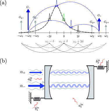
Figure 1: System setup. (a) Sidebands generated by the pump setup discussed in the article (pictorial view) (b) Pumping scheme. The two pumps (blue), generate sidebands at $\pm\delta$ ($\omega_{\mathrm{c}}$ and $\omega_{\mathrm{c}}+2\delta$ in the original frame), while the two probes (grey) generate sidebands respectively at $-2\delta$ and $0$ ($\omega_{\mathrm{c}}-\delta$ and $0$ in the original frame), and at $0$ and $2\delta$ ($\omega_{\mathrm{c}}+\delta$ and $\omega_{\mathrm{c}}+3\delta$ in the original frame). In this work we will focus on the peak generated at $0$( panel (a), green peak).

Setup and equations of motion–

The setup considered here consists of two mechanical resonators dispersively coupled to a single optical cavity. The general Hamiltonian of the (isolated) system can be written as

$$H=\omega_{\mathrm{c}}a^{\dagger}a+ \omega_{1}b_{1}^{\dagger}b_{1}+\omega_{2}b_{2}^{\dagger}b_{2}$$

$$+ g_{0}a^{\dagger}a\left[\left(b_{1}^{\dagger}+b_{1}\right)+\left(b_{2}^{\dagger}+b_{2}\right)\right]$$ (1)

where $a$, $b_{1}$ and $b_{2}$, along with their hermitian conjugates, represent the field operators associated with the cavity and the two mechanical resonators, with resonant frequencies $\omega_{\mathrm{c}}$, $\omega_{1}$ and $\omega_{2}$ respectively. Furthermore, we have assumed that each mechanical resonator is coupled through a radiation-pressure coupling term of strength $g_{0}$. In our scheme the system is strongly driven at frequencies $\omega_{\mathrm{c}}+\omega_{1}$ with a coherent pumping tone of amplitude $\alpha_{+}$ and $\omega_{\mathrm{c}}-\omega_{2}$ with amplitude $\alpha_{-}$ ($G_{\pm}=g_{0}\alpha_{\pm}$). In addition to the driving at $\omega_{\mathrm{c}}\pm\omega_{1,2}$, the cavity driving scheme proposed here comprises four extra detection tones at frequencies $\omega_{\mathrm{c}}+\omega_{1}\pm\delta$ and $\omega_{\mathrm{c}}-\omega_{2}\pm\delta$, with $\delta=\left(\omega_{1}-\omega_{2}\right)/2$ (see Fig. 1).

In the appropriate frame ($\omega_{\mathrm{c}}+\delta$ and $\omega_{\Sigma}=(\omega_{1}+\omega_{2})/2$ for cavity and mechanics respectively), after linearisation around the pumping tones, and neglecting terms rotating at frequencies $\omega\simeq 2\omega_{\Sigma}$ since we assume $\omega_{\Sigma}\gg\kappa$ (rotating-wave approximation), the Hamiltonian can be written as

$$H= -\delta a^{\dagger}a+2\delta\left(b^{\dagger}_{1}b_{1}-b^{\dagger}_{2}b_{2}\right)$$

$$+ \left[G_{+}a^{\dagger}\left(b^{\dagger}_{1}+b^{\dagger}_{2}\right)+G_{-}a^{\dagger}\left(b_{1}+b_{2}\right)+\text{h.c.}\right.$$

$$+ G_{p+}e^{i\delta t}a^{\dagger}\left(b^{\dagger}_{1}+b^{\dagger}_{2}\right)+G_{p-}e^{i\delta t}a^{\dagger}\left(b_{1}+b_{2}\right)+\text{h.c.}$$

$$+ \left.G_{q+}e^{-i\delta t}a^{\dagger}\left(b^{\dagger}_{1}+b^{\dagger}_{2}\right)+G_{q-}e^{-i\delta t}a^{\dagger}\left(b_{1}+b_{2}\right)+\text{h.c.}\right]$$ (2)

with $G_{p,q\pm}=g_{0}\alpha_{p,q\pm}$.

Choosing $G_{+}/G_{-}=G_{p+}/G_{p-}=G_{q+}/G_{q-}$, we can write the quantum Langevin equations (QLEs) associated with the linearized system Hamiltonian (2), in the Fourier domain, as (see A)

$$\chi^{-1}_{\mathrm{c}}\left(\omega+\delta\right)a_{\omega\phantom{,1}}= -i\mathcal{G}\left[\beta_{1\,\omega}+\beta_{2\,\omega}\right]$$

$$-i\mathcal{G}_{\Delta 1}\left[\beta_{1\,\omega-\delta}+\beta_{2\,\omega-\delta}\right]$$

$$-i\mathcal{G}_{\Delta 2}\left[\beta_{1\,\omega+\delta}+\beta_{2\,\omega+\delta}\right]+\sqrt{\kappa}a^{\mathrm{in}}_{\omega}$$

$$\chi^{-1}_{\mathrm{m}}\left(\omega-\delta\right)\beta_{\omega,1}= -i\mathcal{G}^{*}a_{\omega}-i\mathcal{G}^{*}_{\Delta 1}a_{\omega-\delta}$$

$$-i\mathcal{G}^{*}_{\Delta 2}a_{\omega+\delta}+\sqrt{\gamma}\beta^{\mathrm{in}}_{1\,\omega}$$

$$\chi^{-1}_{\mathrm{m}}\left(\omega+\delta\right)\beta_{2\,\omega}= -i\mathcal{G}^{*}a_{\omega}-i\mathcal{G}^{*}_{\Delta 1}a_{\omega-\delta}$$

$$-i\mathcal{G}^{*}_{\Delta 2}a_{\omega+\delta}+\sqrt{\gamma}\beta^{\mathrm{in}}_{2\,\omega}$$ (3)

where $\mathcal{G}=\sqrt{\left|G_{-}\right|^{2}-\left|G_{+}\right|^{2}}$, $\mathcal{G}_{\Delta 1}=\left[G_{-}G_{p-}^{*}-G_{+}G_{p+}^{*}\right]/\mathcal{G}$, $\mathcal{G}_{\Delta 2}=\left[G_{-}G_{q-}^{*}-G_{+}G_{q+}^{*}\right]/\mathcal{G}$ and $\chi_{\mathrm{x}}(\omega)^{-1}=\gamma_{\mathrm{x}}/2-i\omega$ ($\mathrm{x}=1,2$, $\gamma_{1}=\gamma$,$\gamma_{2}=\kappa$). The input field introduced in (3) include contributions both from internal and external noise (see Fig. 1)

$$\sqrt{\kappa}a^{\mathrm{in}}_{\omega}=\sqrt{\kappa_{\mathrm{i}}}a^{\mathrm{in}}_{\mathrm{i}\,\omega}+\sqrt{\kappa_{\mathrm{e}}}a^{\mathrm{in}}_{\mathrm{e}\,\omega}.$$

Most importantly, the mechanical operators

$$\beta_{1\,\omega}=ub_{1\,\omega}+vb_{2\,-\omega}^{\dagger},$$

$$\beta_{2\,\omega}=ub_{2\,\omega}+vb_{1\,-\omega}^{\dagger},$$ (4)

where $u=G_{+}/\sqrt{G_{+}^{2}-G_{-}^{2}}$, $v=G_{-}/\sqrt{G_{+}^{2}-G_{-}^{2}}$, can be regarded as being generated by the action of the two-mode squeezing operator

$$S(r)=\exp\left(r\,b_{\omega,1}b_{\omega,2}-\mathrm{h.c.}\right)$$

with $r=\operatorname{arccosh}u$. $S(r)$ can be shown to give rise to quantum correlations between the mechanical modes, analogously to the situation encountered in the context of quantum optics, e.g. in the case of non-degenerate parametric amplification Walls and Milburn (2008) and thus represents the key ingredient for entanglement generation in the present setup Woolley and Clerk (2014).

Our strategy in the solution of the problem in the presence of both pumping and probing tones, consists now in assuming that $\left|\mathcal{G}\right|\gg\left|\mathcal{G}_{\Delta 1}\right|,\left|\mathcal{G}_{\Delta 2}\right|$, and $\gamma\ll\delta$, treating the probing tones as a perturbation with respect to the driving tones (see B). These conditions allow us to solve for the dynamics of the mechanical resonators as if it was determined by the pumping tone only and independently for each mode.

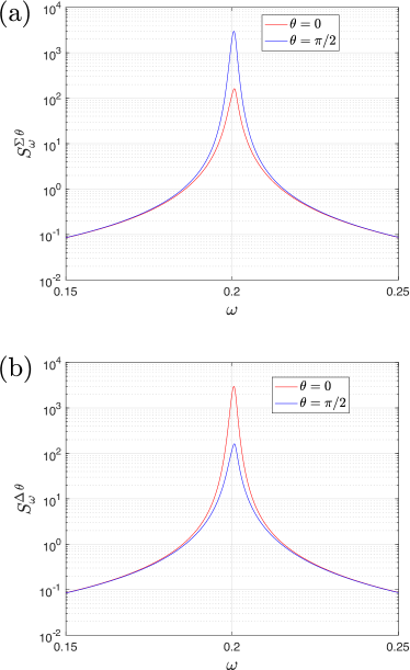
Figure 2: Mechanical spectrum. (a) Spectrum for the symmetrical mechanical quadratures $S_{\omega}^{\Sigma\,\theta}$, for $\theta=0$, (red) and $\theta=\pi/2$ (blue). (b) Spectrum for the antisymmetrical mechanical quadratures $S_{\omega}^{\Delta\,\theta}$ $\theta=0$, (red) and $\theta=\pi/2$ (blue). System parameters: $\delta=0.2$, $G_{-}=4.8\cdot 10^{-2}$, $G_{+}=4.0\cdot 10^{-2}$, $\gamma=1\cdot 10^{-5}$, $n_{\mathbf{m}}=10$, $n_{\mathbf{c}}^{\mathrm{I}}=n_{\mathbf{c}}^{\mathrm{E}}=0.1$, all energies in units of $\kappa$.

In Fig. 2, we have depicted the mechanical noise spectrum, with the following definitions

$$S_{\omega}^{\Sigma\,\theta}=\frac{1}{2}\braket{\left\{\braket{X_{-\omega}^{\Sigma\,\theta},X_{\omega}^{\Sigma\,\theta}}\right\}}$$

$$S_{\omega}^{\Delta\,\theta}=\frac{1}{2}\braket{\left\{\braket{X_{-\omega}^{\Delta\,\theta},X_{\omega}^{\Delta\,\theta}}\right\}}$$ (5)

and

$$X^{\Sigma}_{\omega}\doteq X_{1\,\omega}+X_{2\,\omega}$$

$$X^{\Delta}_{\omega}\doteq X_{1\,\omega}-X_{2\,\omega}$$ (6)

The spectra in Fig. 2 are obtained in the presence of thermal noise both for the cavity ( $\braket{a^{\mathrm{in}}_{\mathrm{I}\,\omega}{a^{in}_{\mathrm{I}\,\omega^{\prime}}}^{\dagger}}=\left(n_{\mathrm{i}}+1\right)\delta_{\omega,\omega^{\prime}}$, $\braket{a^{\mathrm{in}}_{\mathrm{E}\,\omega}{a^{in}_{\mathrm{E}\,\omega^{\prime}}}^{\dagger}}=\left(n_{\mathrm{e}}+1\right)\delta_{\omega,\omega^{\prime}}$), and the mechanical bath ($\braket{b^{\mathrm{in}}_{\mathrm{x}\,\omega}{b^{in}_{\mathrm{x}\,\omega^{\prime}}}^{\dagger}}=\left(n_{\mathrm{m}}+1\right)\delta_{\omega,\omega^{\prime}}$, $\mathrm{x}=1,2$).

The solution of the equations of motion for the mechanical degrees of freedom determines the dynamics of the cavity field, giving rise to the appearance five peaks in the cavity (and output) spectrum. Due to the small value of the mechanical linewidth, it is possible to consider separately each peak induced in the cavity field by the mechanical resonators. In our analysis, we are interested in particular in the peak at $\omega=0$ ($\omega=\omega_{\mathrm{c}}+\delta$ in the original frame), which comprises contributions from the dynamics of both mechanical resonators and, as we will show, contains all the information needed to evaluate the Duan bound. Since for $\omega\simeq 0$ the mechanical contributions to the cavity field are predominantly provided by $\mathcal{G}_{\Delta 1}\beta_{\omega-\delta,2}$ and $\mathcal{G}_{\Delta 2}\beta_{\omega+\delta,1}$, due to the resonance condition in the mechanical equations of motion: for $\omega\simeq 0$, $\beta_{\omega,1}$ is resonant at $\omega+\delta$ and $\beta_{\omega,2}$ at $\omega-\delta$.

Output spectrum–

If homodyne detection is performed on the fluctuations, from Eq. (8), expressing $\beta_{1}$ and $\beta_{2}$ in terms of $b_{1}$ and $b_{2}$, it is possible to monitor the dynamics of the collective mechanical modes through the measurement of the quadratures of the output field, namely (for $\omega\simeq 0$, $\delta\ll\kappa$)

$$X_{\omega}^{\mathrm{out}} \doteq\left(a^{\dagger}e^{i\theta}+ae^{-i\theta}\right)/\sqrt{2}=$$

$$\sqrt{\kappa} \left|\chi_{\mathrm{c}}\left(\omega+\delta\right)\right|\mathcal{G}_{D}\Big{[}(u+v)\cos\theta\left(\cos\varphi\bar{X}^{\Sigma}_{\omega}-\sin\varphi\bar{Y}^{\Delta}_{\omega}\right)$$

$$+(u-v) \sin\theta\left(\cos\varphi\bar{Y}^{\Delta}_{\omega}+\sin\varphi\bar{X}^{\Delta}_{\omega}\right)\Big{]}+\left[\kappa\chi_{\mathrm{c}}\left(\omega+\delta\right)-1\right]X^{\mathrm{in}}_{\omega}$$ (7)

where the dynamics of the collective mechanical modes is encoded in the frequency-shifted quadrature operators $\bar{X}^{\Sigma}_{\omega}$, $\bar{Y}^{\Sigma}_{\omega}$ and $\bar{X}^{\Delta}_{\omega}$, $\bar{Y}^{\Delta}_{\omega}$ defined by

$$\bar{X}^{\Sigma}_{\omega}\doteq\bar{X}_{1\,\omega}+\bar{X}_{2\,\omega}$$

$$\bar{X}^{\Delta}_{\omega}\doteq\bar{X}_{1\,\omega}-\bar{X}_{2\,\omega}$$ (8)

with

$$\bar{X}_{\mathrm{1}\,\omega} \doteq\left(b^{\dagger}_{\mathrm{1}\,-\omega+\delta}+b_{\mathrm{1}\,\omega+\delta}\right)/\sqrt{2}$$

$$\bar{X}_{\mathrm{2}\,\omega} \doteq\left(b^{\dagger}_{\mathrm{2}\,-\omega-\delta}+b_{\mathrm{2}\,\omega-\delta}\right)/\sqrt{2},$$ (9)

with analogous definitions holding for the quadratures $\bar{Y}_{1\,\omega}$ and $\bar{Y}_{2\,\omega}$. Note that the frequency-shifted quadrature operators defined above, do not directly correspond to the usual quadrature operators. In the time domain, the operators defined in (9) acquire a nontrivial time dependence, for instance we have that

$$\bar{X}_{1\,t}=b_{\mathrm{t}}e^{i\delta t}+b^{\dagger}_{\mathrm{t}}e^{-i\delta t}$$

and thus correspond to the mechanical quadratures for $\delta=0$ only. While one cannot directly relate the frequency-shifted quadrature operators to the regular ones, for each pair of orthogonal quadratures, the uncertainties associated with the collective quadratures of the mechanical motion, fulfil the following relation

$$\braket{\Delta\bar{X}_{\Sigma}^{2}}+\braket{\Delta\bar{Y}_{\Delta}^{2}}=\braket{\Delta X_{\Sigma}^{2}}+\braket{\Delta Y_{\Delta}^{2}},$$ (10)

which, crucially, allows us to establish the link between the output spectrum and the spectrum of the collective mechanical quadratures. Therefore, the knowledge of one pair of orthogonal frequency-shifted mechanical quadratures allows one to deduce the value of the corresponding pair of regular quadratures and, consequently, to infer the value of the Duan quantity from the spectrum of the output field.

In the derivation of Eq. (7), we have chosen the average phase of the detection tones as the phase reference with respect to which both the phases of the probing tones $\mathcal{G}_{\Delta_{1}}$ and $\mathcal{G}_{\Delta_{2}}$ ($\pm\varphi$) as well as the homodyne detection phase $\theta$ are referred. From Eq. (7), it is possible to relate the output spectrum $S^{\mathrm{out}\,\theta}_{\omega}$ to the spectrum of the frequency-shifted mechanical quadratures as

$$S^{\mathrm{out}\,\theta}_{\omega}=\mathcal{G}^{2}_{D}\left|\chi_{\mathrm{c}}(\delta)\right|^{2}$$ (11)

$$\left\{\left(u+v\right)^{2}\left[\left(\cos\theta\cos\varphi\right)^{2}\bar{S}_{\omega}^{\Sigma\,0}+\left(\cos\theta\sin\varphi\right)^{2}\bar{S}_{\omega}^{\Delta\,\pi/2}\right]\right.$$

$$\left.+\left(u-v\right)^{2}\left[\left(\sin\theta\cos\varphi\right)^{2}\bar{S}_{\omega}^{\Sigma\,\pi/2}+\left(\sin\theta\sin\varphi\right)^{2}\bar{S}_{\omega}^{\Delta\,0}\right]\right\}$$

$$+B^{\mathrm{in}}+C_{\omega}^{\mathrm{in}}\cos\left[2\phi\right]$$ (12)

(see the C for the derivation of the output noise spectrum $S^{\mathrm{out}\,\theta}_{\omega}$, and the definitions of $B^{\mathrm{in}}$ and $C_{\omega}^{\mathrm{in}}$).

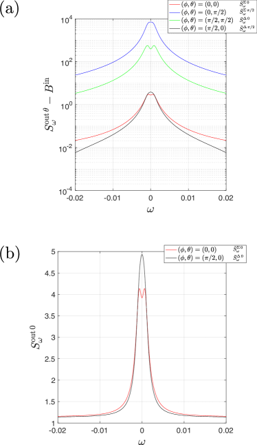
Figure 3: Output spectrum. (a) Spectrum for the output field for the four relevant combinations of $\left(\phi,\theta\right)$. Note the two-mode squeezing effect, indicated by the difference in the noise spectra for $\left(0,0\right)$ and $\left(0,\pi/2\right)$, and $\left(\pi/2,0\right)$ and $\left(\pi/2,\pi/2\right)$, respectively. (b) Same as in (a) focus on the spectra for $\left(\phi,\theta\right)=(0,0)$ and $\left(\phi,\theta\right)=(\pi/2,0)$ –note here the linear scale;the base level corresponds to the pure cavity response. For each value of the pair $\left(\phi,\theta\right)$, we have indicated the corresponding shifted mechanical noise spectrum. Physical parameters same as in Fig. 2.

Eq. (8) expresses the possibility to access the collective mechanical noise spectra $\bar{S}_{\omega}^{\Sigma\,0}$, $\bar{S}_{\omega}^{\Sigma\,\pi/2}$, $\bar{S}_{\omega}^{\Delta\,0}$, $\bar{S}_{\omega}^{\Delta\,\pi/2}$, by changing the relative phase of the detection tones $\varphi$ and the phase of the homodyne detector $\theta$.

The measurement strategy leading to the determination of the Duan quantity consists in the measurement of the output spectrum for four different values of $\left(\theta,\varphi\right)=\left(0,0\right)$, $\left(0,\pi/2\right)$, $\left(\pi/2,0\right)$, $\left(\pi/2,\pi/2\right)$, yielding

$$\left.S^{\mathrm{out}\,0}_{\omega}\right|_{\varphi=0} = \left(u+v\right)\bar{S}_{\omega}^{\Sigma\,0}+C_{\omega}^{\mathrm{in}}$$

$$\left.S^{\mathrm{out}\,0}_{\omega}\right|_{\varphi=\pi/2} = \left(u+v\right)\bar{S}_{\omega}^{\Delta\,\pi/2}-C_{\omega}^{\mathrm{in}}$$

$$\left.S^{\mathrm{out}\,\pi/2}_{\omega}\right|_{\varphi=0} = \left(u-v\right)\bar{S}_{\omega}^{\Sigma\,\pi/2}+C_{\omega}^{\mathrm{in}}$$

$$\left.S^{\mathrm{out}\,\pi/2}_{\omega}\right|_{\varphi=\pi/2} = \left(u-v\right)\bar{S}_{\omega}^{\Delta\,0}-C_{\omega}^{\mathrm{in}}.$$ (13)

Having in mind the relation established by Eq. (10) The Duan quantity can then be determined as the sum of the appropriate output quadrature spectra as determined in Eqs. (13). The output spectrum therefore provides a measurement of the collective mechanical quadratures induced by the pumping tones $\alpha_{\pm}$, disregarding higher-order effects induced by the detection tones. As detailed in B, for $\omega\simeq 0$ the correction to the dynamics of the mechanical resonators due to the detection tones is of the order $\left(\mathcal{G}_{D}/\mathcal{G}\right)^{2}$, and thus can be safely neglected for a suitable choice of readout tones.

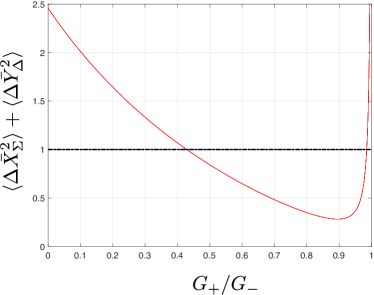
Figure 4: Duan quantity as obtained from the shifted mechanical operators as a function of the ratio $G_{+}/G_{-}$, (with $G_{-}$ kept fixed), showing that for a ratio $G_{+}/G_{-}$ between $\simeq 0.45$ and $\simeq 0.99$, the mechanical resonators are entangled . Other physical parameters same as in Fig. 2

.

In the limit $\kappa\gg\delta,\mathcal{G}\gg\gamma$, the quantity given in Eq. (10) can be written as

$$\braket{\Delta\bar{X}_{\Sigma}^{2}}+\braket{\Delta\bar{Y}_{\Delta}^{2}}=$$

$$\left[\gamma\kappa\left(n_{\mathrm{m}}+\frac{1}{2}\right)+4\left(G_{-}^{2}+G_{+}^{2}\right)\left(n_{\mathrm{c}}+\frac{1}{2}\right)\right]/\left[2(G_{-}^{2}-G_{+}^{2})\right]$$ (14)

(see C for the full exact expression), which corresponds to the approximate formula given in Woolley and Clerk (2014) for the Duan quantity in the adiabatic limit.

The detection scheme proposed here represents a somewhat idealised setup. A first apporximation in our approach is represented by the rotating-wave approximation. Considering that that discarded terms in performing the rotating wave approximation are of the order on $\sim\left(\kappa/\omega_{\mathrm{m}}\right)^{2}$, reaching a range of experimental parameters in which this approximation does not seem to represent an insurmountable experimental challenge (see e.g. Pirkkalainen et al. (2015), where $\kappa/\omega_{\mathrm{m}}\simeq 0.05$).

The most relevant source of non-ideality is probably represented by the presence of parametric modulation terms to the dynamics of the cavity. This effect was observed in the context of the optomechanical generation and detection of mechanical squeezing Wollman et al. (2015); Pirkkalainen et al. (2015) and is likely to affect the detection of mechanical entanglement as well.

Among other non-idealities likely encountered in the specific experimental realisation of the detection scheme discussed here, it is worth mentioning that the two mechanical resonators are inevitably not identical and the thermal baths to which they are coupled are not necessarily at the same temperature. The most severe constraint posed by the difference between the two mechanical resonators seems to be posed by the different value of the bare optomechanical coupling $g_{0}$, which however can be compensated by a suitably engineered pumping scheme (see e.g. Woolley and Clerk (2014)).

We have proposed here a potential scheme for the detection of entanglement between mechanical resonators coupled to a common optical cavity, establishing a straightforward setup for the quantification of such entanglement in terms of the Duan quantity. Its feasibility is within the framework of current experimental capabilities.

The author would like to thank Mika Sillanpää and Tero Heikkilä for useful discussions. This work was supported by the Academy of Finland (Contract No. 27545).

Appendix A Derivation of the equations of motion

In the appropriate frame ($\omega_{\mathrm{c}}+\delta$ and $\omega_{\Sigma}=(\omega_{1}+\omega_{2})/2$ for cavity and mechanics respectively), and invoking the rotating-wave approximation, the Hamiltonian given in Eq. (2) of the main text can be written as

$$H= -\delta a^{\dagger}a+\delta\left(b^{\dagger}_{1}b_{1}-b^{\dagger}_{2}b_{2}\right)$$

$$+ \left[G_{+}a^{\dagger}\left(b^{\dagger}_{1}+b^{\dagger}_{2}\right)+G_{-}a^{\dagger}\left(b_{1}+b_{2}\right)+\text{h.c.}\right.$$

$$+ G_{p+}e^{i\delta t}a^{\dagger}\left(b^{\dagger}_{1}+b^{\dagger}_{2}\right)+G_{p-}e^{i\delta t}a^{\dagger}\left(b_{1}+b_{2}\right)+\text{h.c.}$$

$$+ \left.G_{q+}e^{-i\delta t}a^{\dagger}\left(b^{\dagger}_{1}+b^{\dagger}_{2}\right)+G_{q-}e^{-i\delta t}a^{\dagger}\left(b_{1}+b_{2}\right)+\text{h.c.}\right]$$ (15)

with $\delta=\left(\omega_{1}-\omega_{2}\right)/2$. From the Hamiltonian (15), it is possible to write down the quantum Langevin equations for cavity and mechanical degrees of freedom as

$$\dot{a}= -i\delta a-i\sqrt{2}\left[\left(G_{+}b^{\dagger}_{\Sigma}+G_{-}b_{\Sigma}\right)\right.$$

$$\hphantom{-i\delta a-i\sqrt{2}}+\left(G_{p+}e^{i\delta t}b_{\Sigma}^{\dagger}+G_{p-}e^{i\delta t}b_{\Sigma}\right)$$

$$\hphantom{-i\delta a-i\sqrt{2}}\left.+\left(G_{q+}e^{i\delta t}b_{\Sigma}^{\dagger}+G_{q-}e^{i\delta t}b_{\Sigma}\right)\right]$$

$$\dot{b}_{\Sigma}= -i\delta b_{\Delta}-i\sqrt{2}\left[\left(G_{+}a^{\dagger}+G^{*}_{-}a\right)\right.$$

$$\hphantom{-i\delta b_{\Delta}-i\sqrt{2}}+\left(G_{p+}e^{i\delta t}a^{\dagger}+G^{*}_{p-}e^{-i\delta t}a\right)$$

$$\hphantom{-i\delta b_{\Delta}-i\sqrt{2}}\left.+\left(G_{q+}e^{-i\delta t}a^{\dagger}+G^{*}_{q-}e^{i\delta t}a\right)\right]$$

$$\dot{b}_{\Delta}= -i\delta b_{\Sigma}$$ (16)

where we have defined $b_{\Sigma}=\left(b_{1}+b_{2}\right)/\sqrt{2}$, $b_{\Delta}=\left(b_{1}-b_{2}\right)/\sqrt{2}$. If we now write the EOM for the linear combination $\left(G_{-}b_{\Sigma,\Delta}+G_{+}b_{\Sigma,\Delta}^{\dagger}\right)$, from Eq. (16) we can write

$$\left(G_{-}\dot{b}_{\Sigma}+G_{+}\dot{b}_{\Sigma}^{\dagger}\right)=$$

$$-i\delta\left(G_{-}b_{\Delta}-G_{+}b_{\Delta}^{\dagger}\right)$$

$$-i\sqrt{2}\left[\left(\left|G_{-}\right|^{2}a-\left|G_{+}\right|^{2}a+\cancel{G_{-}G_{+}a^{\dagger}}-\cancel{G_{-}G_{+}a^{\dagger}}\right)\right.$$

$$\hphantom{-i\sqrt{2}\Big{[}}+\left(G_{-}G_{p-}^{*}e^{-i\delta t}a-G_{+}G_{p+}e^{-i\delta t}a\right.$$

$$\hphantom{-i\sqrt{2}\Big{[}\Big{[}\Big{[}}\left.+\cancel{G_{-}G_{p+}e^{i\delta t}a^{\dagger}}-\cancel{G_{+}G_{p-}e^{i\delta t}a^{\dagger}}\right)$$

$$\hphantom{-i\sqrt{2}\Big{[}}+\left(G_{-}G_{q-}^{*}e^{i\delta t}a-G_{+}G_{q+}e^{i\delta t}a\right.$$

$$\hphantom{-i\sqrt{2}\Big{[}\Big{[}\Big{[}}\left.\left.+\cancel{G_{-}G_{q+}e^{-i\delta t}a^{\dagger}}-\cancel{G_{+}G_{q-}e^{-i\delta t}a^{\dagger}}\right)\right].$$ (17)

and, analogously,

$$\left(G_{-}\dot{b}_{\Delta}-G_{+}\dot{b}_{\Delta}^{\dagger}\right)=-i\delta\left(G_{-}b_{\Sigma}+G_{+}b_{\Sigma}^{\dagger}\right)$$ (18)

The cancellations on the second and third line of Eq. (17), needed to recast the problem in terms of Bogolyubov modes, occur only if $G_{p+}/G_{p-}=G_{q+}/G_{q\,-}=G_{+}/G_{-}$. In this case,

$$\dot{a}= -i\delta a$$

$$-i\sqrt{2}\left[\mathcal{G}^{*}+\mathcal{G}^{*}_{\Delta 1}e^{i\delta t}+\mathcal{G}^{*}_{\Delta 2}e^{-i\delta t}\right]\beta_{\Sigma}$$

$$\dot{\beta}_{\Sigma}= -i\delta\beta_{\Delta}$$

$$-i\sqrt{2}\left[\mathcal{G}+\mathcal{G}_{\Delta 1}e^{-i\delta t}+\mathcal{G}_{\Delta 2}e^{i\delta t}\right]a$$

$$\dot{\beta}_{\Delta}= -i\delta\beta_{\Sigma}$$ (19)

where we have adopted the definitions

$$\beta_{\Sigma}=ub_{\Sigma}+v{b_{\Sigma}}^{\dagger}$$

$$\beta_{\Delta}=ub_{\Delta}-v{b_{\Delta}}^{\dagger}$$

$$\mathcal{G}=\sqrt{\left|G_{-}\right|^{2}-\left|G_{+}\right|^{2}}$$

$$\mathcal{G}_{\Delta 1}=\left[G_{-}G_{p-}^{*}-G_{+}G_{p+}^{*}\right]/\mathcal{G}$$

$$\mathcal{G}_{\Delta 2}=\left[G_{-}G_{q-}^{*}-G_{+}G_{q+}^{*}\right]/\mathcal{G}.$$ (20)

In order to ensure that the mechanical operators on the rhs of Eq. (16) can be all expressed in terms of the same Bogolyubov operator, we have to verify under what conditions the following three (in principle different) transformations

$$G_{-}b_{\Sigma}+G_{+}b^{\dagger}_{\Sigma}=\mathcal{G}\left(ub_{\Sigma}+vb^{\dagger}_{\Sigma}\right)$$

$$G_{p-}b_{\Sigma}+G_{p+}b^{\dagger}_{\Sigma}=\mathcal{G}_{\Delta 1}\left(u^{\prime}b_{\Sigma}+v^{\prime}b^{\dagger}_{\Sigma}\right)$$

$$G_{q-}b_{\Sigma}+G_{q+}b^{\dagger}_{\Sigma}=\mathcal{G}_{\Delta 2}\left(u^{\prime\prime}b_{\Sigma}+v^{\prime\prime}b^{\dagger}_{\Sigma}\right)$$

coincide, having set

$$u\hphantom{{}^{\prime\prime}}=\frac{G_{-}}{\mathcal{G}}, v\hphantom{{}^{\prime\prime}}=\frac{G_{+}}{\mathcal{G}}$$

$$u^{\prime}\hphantom{{}^{\prime}}=\frac{G_{p-}}{\mathcal{G}_{\Delta 1}}, v^{\prime}\hphantom{{}^{\prime}}=\frac{G_{p+}}{\mathcal{G}_{\Delta 1}}$$

$$u^{\prime\prime}=\frac{G_{q-}}{\mathcal{G}_{\Delta 2}}, v^{\prime\prime}=\frac{G_{q+}}{\mathcal{G}_{\Delta 2}}.$$ (22)

It turns out that the condition $G_{p+}/G_{p-}=G_{q+}/G_{q\,-}=G_{+}/G_{-}$ is a sufficient condition to determine $u=u^{\prime}=u^{\prime\prime}$ and $v=v^{\prime}=v^{\prime\prime}$. In our analysis we have set the reference phase to be given by the pump tones $G_{+}$ and $G_{-}$. Focusing on $u^{\prime}$, we have

$$\frac{\mathcal{G}^{2}}{\left|G_{+}\right|} =\left|G_{+}-G_{-}\frac{G_{-}^{*}}{G_{+}^{*}}\right|=\left|G_{+}-G_{-}\frac{G_{p-}^{*}}{G_{p+}^{*}}\right|$$

$$=\left|\frac{G_{+}G^{*}_{p+}-G_{-}G^{*}_{p-}}{G_{p+}^{*}}\right|$$

$$=\left|\frac{\mathcal{G}_{\Delta 1}}{G_{p+}^{*}}\right|\implies u=u^{\prime}$$ (23)

and analogously for $v^{\prime}$, $u^{\prime\prime}$ and $v^{\prime\prime}$. Defining

$$\beta_{1}= \frac{\beta_{\Sigma}+\beta_{\Delta}}{\sqrt{2}}=ub_{1}+vb_{2}^{\dagger}$$

$$\beta_{2}= \frac{\beta_{\Sigma}-\beta_{\Delta}}{\sqrt{2}}=ub_{2}+vb_{1}^{\dagger},$$ (24)

we can write the quantum Langevin equations of motion induced by the Hamiltonian (15) in the Fourier domain as

$${\left(\chi^{\mathrm{c}}_{\omega+\delta}\right)}^{-1}a_{\omega}=-i\mathcal{G}\left[\beta_{1\,\omega}+\beta_{2\,\omega}\right]$$

$$\hphantom{{(\chi^{\mathrm{c}}_{\omega+\delta})}^{-1}a_{\omega}=}-i\mathcal{G}_{\Delta 1}\left[\beta_{1\,\omega-\delta}+\beta_{2\,\omega-\delta}\right]$$

$$\hphantom{{(\chi^{\mathrm{c}}_{\omega+\delta})}^{-1}a_{\omega}=}-i\mathcal{G}_{\Delta 2}\left[\beta_{2\,\omega+\delta}+\beta_{2\,\omega+\delta}\right]$$

$$\hphantom{{(\chi^{\mathrm{c}}_{\omega+\delta})}^{-1}a_{\omega}=}+\sqrt{\kappa_{\mathrm{e}}}a^{\mathrm{in}}_{\mathrm{E}\,\omega}+\sqrt{\kappa_{\mathrm{i}}}a^{\mathrm{in}}_{\mathrm{I}\,\omega}$$

$${\left(\chi^{\mathrm{m}}_{\omega-\delta}\right)}^{-1}\beta_{1\,\omega}=-i\mathcal{G}^{*}a_{\omega}$$

$$\hphantom{{\left(\chi^{\mathrm{m}}_{\omega+\delta}\right)}^{-1}\beta_{2\,\omega}=}-i\mathcal{G}^{*}_{\Delta 1}a_{\omega-\delta}-i\mathcal{G}^{*}_{\Delta 2}a_{\omega+\delta}+\sqrt{\gamma}\beta^{\mathrm{in}}_{1\,\omega}$$

$${\left(\chi^{\mathrm{m}}_{\omega+\delta}\right)}^{-1}\beta_{2\,\omega}=-i\mathcal{G}^{*}a_{\omega}$$

$$\hphantom{{\left(\chi^{\mathrm{m}}_{\omega+\delta}\right)}^{-1}\beta_{2\,\omega}=}-i\mathcal{G}^{*}_{\Delta 1}a_{\omega-\delta}-i\mathcal{G}^{*}_{\Delta 2}a_{\omega+\delta}+\sqrt{\gamma}\beta^{\mathrm{in}}_{2\,\omega}$$ (25)

which correspond to Eq. (3) of the main text.

Appendix B Equations of motion: perturbative solution

In the following we derive the solution of the equations of motion around $\omega\simeq 0$, treating the probing tones $\mathcal{G}_{\Delta 1}$ and $\mathcal{G}_{\Delta 2}$ perturbatively. The solution that we obtain for the output field is then used to determine the output noise spectrum, from which, in turn, it is possible to deduce the mechanical modes dynamics. The solution of the equations of motion (25), considering that $\mathcal{G}\ll\left|\mathcal{G}_{\Delta 1}\right|=\left|\mathcal{G}_{\Delta 2}\right|$, can be obtained with the aid of perturbation theory. Defining

$$\mathcal{G}_{\Delta 1}=\lambda e^{\phi_{1}}\mathcal{G}_{D}$$

$$\mathcal{G}_{\Delta 2}=\lambda e^{\phi_{2}}\mathcal{G}_{D}$$

we can formally write the solution for $a_{\omega}$, $\beta_{1\,\omega}$, $\beta_{2\,\omega}$ as

$$a_{\omega}=a_{\omega}^{(0)}+\lambda a_{\omega}^{(1)}+\lambda^{2}a_{\omega}^{(2)}+O(\lambda^{3})$$

$$\beta_{\omega,1}=\beta_{\omega,1}^{(0)}+\lambda\beta_{1\,\omega}^{(1)}+\lambda^{2}\beta_{1\,\omega}^{(2)}+O(\lambda^{3})$$

$$\beta_{2\,\omega}=\beta_{2\,\omega}^{(0)}+\lambda\beta_{2\,\omega}^{(1)}+\lambda^{2}\beta_{2\,\omega}^{(2)}+O(\lambda^{3}).$$ (26)

Substituting the perturbative expression given by Eq. (26), Eqs. (25) can be solved order-by-order in $\lambda$,

$${\left(\chi^{\mathrm{c}}_{\omega+\delta}\right)}^{-1}a^{(n)}_{\omega}=-i\mathcal{G}\left[\beta^{(n)}_{1\,\omega}+\beta^{(n)}_{2\,\omega}\right]-i\lambda\mathcal{G}_{D}\left\{e^{i\phi 1}\left[\beta^{(n-1)}_{1\,\omega-\delta}+\beta^{(n-1)}_{2\,\omega-\delta}\right]+e^{i\phi 2}\left[\beta^{(n-1)}_{1\,\omega+\delta}+\beta^{(n-1)}_{2\,\omega+\delta}\right]\right\}+\sqrt{\kappa_{\mathrm{e}}}a^{\mathrm{in}}_{\mathrm{E}\,\omega}+\sqrt{\kappa_{\mathrm{i}}}a^{\mathrm{in}}_{\mathrm{I}\,\omega}$$

$${\left(\chi^{\mathrm{m}}_{\omega-\delta}\right)}^{-1}\beta^{(n)}_{1\omega}=-i\mathcal{G}^{*}a^{(n)}_{\omega}+i\lambda\mathcal{G}_{D}\left[e^{-i\phi 1}a^{(n-1)}_{\omega-\delta}+e^{-i\phi 2}a^{(n-1)}_{\omega+\delta}\right]+\sqrt{\gamma}\beta^{\mathrm{in}}_{1\,\omega}$$

$${\left(\chi^{\mathrm{m}}_{\omega+\delta}\right)}^{-1}\beta^{(n)}_{2\omega}=-i\mathcal{G}^{*}a^{(n)}_{\omega}+i\lambda\mathcal{G}_{D}\left[e^{-i\phi 1}a^{(n-1)}_{\omega-\delta}+e^{-i\phi 2}a^{(n-1)}_{\omega+\delta}\right]+\sqrt{\gamma}\beta^{\mathrm{in}}_{2\,\omega}.$$ (27)

The $0$-th order term of Eq. (27) is represented by the equations governing the 2-pump driving scheme, in the absence of detection tones which can be readily solved to give

$$a_{\omega}^{(0)}=\chi^{\mathrm{c}}_{\omega+\delta}\left[-i\mathcal{G}\left(\beta_{\omega,1}^{(0)}+\beta_{\omega,2}^{(0)}\right)+\sqrt{\kappa_{\mathrm{e}}}a^{\mathrm{in}}_{\mathrm{E}\,\omega}+\sqrt{\kappa_{\mathrm{i}}}a^{\mathrm{in}}_{\mathrm{I}\,\omega}\right]$$

$$\beta^{(0)}_{1\,\omega}=\chi_{\omega}^{\mathrm{e}1}\sqrt{\gamma}\beta^{\mathrm{in}}_{1\,\omega}-i\mathcal{G}\chi_{\omega}^{\mathrm{x}1}\left(\sqrt{\kappa_{\mathrm{e}}}a^{\mathrm{in}}_{\mathrm{E}\,\omega}+\sqrt{\kappa_{\mathrm{i}}}a^{\mathrm{in}}_{\mathrm{I}\,\omega}\right)$$

$$\beta^{(0)}_{2\,\omega}=\chi_{\omega}^{\mathrm{e}2}\sqrt{\gamma}\beta^{\mathrm{in}}_{2\,\omega}-i\mathcal{G}\chi_{\omega}^{\mathrm{x}2}\left(\sqrt{\kappa_{\mathrm{e}}}a^{\mathrm{in}}_{\mathrm{E}\,\omega}+\sqrt{\kappa_{\mathrm{i}}}a^{\mathrm{in}}_{\mathrm{I}\,\omega}\right)$$ (28)

where

$$\chi^{\mathrm{e}1}_{\omega}= \frac{\chi^{\mathrm{m}}_{\omega-\delta}}{1+\mathcal{G}^{2}\chi^{\mathrm{c}}_{\omega+\delta}\chi^{\mathrm{m}}_{\omega-\delta}}$$

$$\chi^{\mathrm{e}2}_{\omega}= \frac{\chi^{\mathrm{m}}_{\omega+\delta}}{1+\mathcal{G}^{2}\chi^{\mathrm{c}}_{\omega+\delta}\chi^{\mathrm{m}}_{\omega+\delta}}$$

$$\chi^{x1}_{\omega}= \frac{\chi^{\mathrm{c}}_{\omega+\delta}\chi^{\mathrm{m}}_{\omega-\delta}}{1+\mathcal{G}^{2}\chi^{\mathrm{c}}_{\omega+\delta}\chi^{\mathrm{m}}_{\omega-\delta}}$$

$$\chi^{\mathrm{x}2}_{\omega}= \frac{\chi^{\mathrm{c}}_{\omega+\delta}\chi^{\mathrm{m}}_{\omega+\delta}}{1+\mathcal{G}^{2}\chi^{\mathrm{c}}_{\omega+\delta}\chi^{\mathrm{m}}_{\omega+\delta}}$$ (29)

The assumption $\gamma\ll\delta$ allows us to recognise that $\beta^{0}_{1\,\omega}$ and $\beta^{0}_{2\,\omega}$ are peaked around $\omega\simeq\delta$ and $\omega\simeq-\delta$ respectively, while $a_{\omega}^{0}$ exhibits a double-peak structure for $\omega\simeq\pm\delta$.

The solution given by (28), allows us to write the first-order approximation of the system equations of motion ($n=1$ in Eq. (27)). The considerations concerning the peak structure of the $0$-th order equations - essentially because $\chi_{\mathrm{m}}\left(\omega\right)\sim\delta_{\omega}$ –, allow us to write the first order approximation for the cavity field and the mechanics as

1. $\omega\simeq 0$

   $$a_{\omega}^{1}=-i\lambda\mathcal{G}_{D}\chi^{\mathrm{c}}_{\omega+\delta}\left[e^{i\phi 1}\beta_{\omega-\delta,2}^{0}+e^{i\phi 2}\beta_{\omega+\delta,1}^{0}\right]$$

   $$\beta^{1}_{1\,\omega}=0$$

   $$\beta^{1}_{2\,\omega}=0$$

   The value of the first-order correction to the cavity field, can be expressed in terms of the input field

   $$a_{\omega}^{(1)}=-i\lambda\mathcal{G}_{D}\chi^{\mathrm{c}}_{\omega+\delta}\left[e^{i\phi 1}\left\{\chi_{\omega-\delta}^{\mathrm{e}2}\sqrt{\gamma}\beta^{\mathrm{in}}_{\omega-\delta,2}-i\mathcal{G}\chi_{\omega-\delta}^{\mathrm{x}2}\left(\sqrt{\kappa_{i}}a^{\mathrm{in}}_{\mathrm{I}\,\omega-\delta}+\sqrt{\kappa_{e}}a^{\mathrm{in}}_{\mathrm{E}\,\omega-\delta}\right)\right\}\right.+$$

   $$\hphantom{a_{\omega}^{(1)}=-i\lambda\mathcal{G}_{D}\chi^{\mathrm{c}}_{\omega+\delta}\big{[}}\left.e^{i\phi 2}\left\{\chi_{\omega+\delta}^{\mathrm{e}1}\sqrt{\gamma}\beta^{\mathrm{in}}_{\omega+\delta,1}-i\mathcal{G}\chi_{\omega+\delta}^{\mathrm{x}1}\left(\sqrt{\kappa_{i}}a^{\mathrm{in}}_{\mathrm{I}\,\omega+\delta}+\sqrt{\kappa_{e}}a^{\mathrm{in}}_{\mathrm{E}\,\omega+\delta}\right)\right\}\right].$$ (31)

   On the other hand, Eq. (LABEL:eq:4x) can be shown to encode the relevant information about the mechanical quadratures

   $$a_{\omega}^{(1)}= -i\lambda\mathcal{G}_{D}\chi^{\mathrm{c}}_{\omega+\delta}\frac{e^{i\Phi}}{\sqrt{2}}$$

   $$\left\{\left(u+v\right)\left[\cos\varphi\left(\bar{X}_{1\,\omega}+\bar{X}_{2\,\omega}\right)\right.\right.$$

   $$\left.\hphantom{(u+v)}-\sin\varphi\left(\bar{Y}_{1\,\omega}-\bar{Y}_{2\,\omega}\right)\right]$$

   $$+\left(u-v\right)\left[\cos\varphi\left(\bar{Y}_{2\,\omega}+\bar{Y}_{2\,\omega}\right)\right.$$

   $$\left.\left.\hphantom{(u-v)}+\sin\varphi\left(\bar{X}_{1\,\omega}-\bar{X}_{2\,\omega}\right)\right]\right\}$$ (32)

   where $\Phi=\phi_{1}+\phi_{2}$ and $\varphi=\phi_{1}-\phi_{2}$.

   From Eq. (1) it is possible to notice that $a_{\omega}^{1}$ does not depend on the value of the input fields at $\omega=0$, implying that the backaction term, to this order, will not give rise to any interference contribution with the zeroth-order cavity field.

2. $\omega\simeq\delta$

   $$a_{\omega}^{(1)}=-\lambda\mathcal{G}_{D}\frac{\mathcal{G}\chi^{\mathrm{c}}_{\omega+\delta}\chi^{\mathrm{m}}_{\omega-\delta}}{1+\mathcal{G}^{2}\chi^{\mathrm{c}}_{\omega+\delta}\chi^{\mathrm{m}}_{\omega-\delta}}\left(e^{-i\phi_{1}}a_{\omega-\delta}^{(0)}+e^{-i\phi_{2}}a_{\omega+\delta}^{(0)}\right)$$

   $$\beta^{(1)}_{1\,\omega}=-i\lambda\mathcal{G}_{D}^{*}\chi^{\mathrm{m}}_{\omega-\delta}\left[1-\frac{\mathcal{G}^{2}\chi^{\mathrm{c}}_{\omega+\delta}\chi^{\mathrm{m}}_{\omega-\delta}}{1+\mathcal{G}^{2}\chi^{\mathrm{c}}_{\omega+\delta}\chi^{\mathrm{m}}_{\omega-\delta}}\right]\left(e^{-i\phi_{1}}a_{\omega-\delta}^{(0)}+e^{-i\phi_{2}}a_{\omega+\delta}^{(0)}\right)$$

   $$\beta^{(1)}_{2\,\omega}=0$$

3. $\omega\simeq-\delta$

   $$a_{\omega}^{(1)}=-\lambda\mathcal{G}_{D}\frac{\mathcal{G}\chi^{\mathrm{c}}_{\omega+\delta}\chi^{\mathrm{m}}_{\omega+\delta}}{1+\mathcal{G}^{2}\chi^{\mathrm{c}}_{\omega+\delta}\chi^{\mathrm{m}}_{\omega+\delta}}\left(e^{-i\phi_{1}}a_{\omega-\delta}^{(0)}+e^{-i\phi_{2}}a_{\omega+\delta}^{(0)}\right)$$

   $$\beta^{(1)}_{1\,\omega}=0$$

   $$\beta^{(1)}_{2\,\omega}=-i\lambda\mathcal{G}_{D}^{*}\chi^{\mathrm{m}}_{\omega+\delta}\left[1-\frac{\mathcal{G}^{2}\chi^{\mathrm{c}}_{\omega+\delta}\chi^{\mathrm{m}}_{\omega+\delta}}{1+\mathcal{G}^{2}\chi^{\mathrm{c}}_{\omega+\delta}\chi^{\mathrm{m}}_{\omega+\delta}}\right]\left(e^{-i\phi_{1}}a_{\omega-\delta}^{(0)}+e^{-i\phi_{2}}a_{\omega+\delta}^{(0)}\right)$$

The same strategy can be applied to determine the second-order approximation to the cavity field around $\omega\simeq 0$ ($n=2$ in Eq. (27)), giving

$$a_{\omega}^{(2)}=-i\lambda\mathcal{G}_{D}\chi^{\mathrm{c}}_{\omega+\delta}\left(e^{i\phi_{1}}\beta_{2\,\omega-\delta}^{(1)}+e^{i\phi_{2}}\beta_{1\,\omega+\delta}^{(1)}\right)$$ (35)

and, in terms of $0$-th order approximation,

$$a_{\omega}^{(2)}=-\lambda^{2}\mathcal{G}_{D}^{2}\chi^{\mathrm{m}}_{\omega} \left\{\left[1-\frac{\mathcal{G}^{2}\chi^{\mathrm{c}}_{\omega}\chi^{\mathrm{m}}_{\omega}}{1+\mathcal{G}^{2}\chi^{\mathrm{c}}_{\omega}\chi^{\mathrm{m}}_{\omega}}\right]\left(a_{\omega-2\delta}^{(0)}+e^{i(\phi_{1}-\phi_{2})}a_{\omega}^{(0)}\right)\right.$$

$$+ \hphantom{\Bigg{[}}\left.\left[1-\frac{\mathcal{G}^{2}\chi^{\mathrm{c}}_{\omega+2\delta}\chi^{\mathrm{m}}_{\omega}}{1+\mathcal{G}^{2}\chi^{\mathrm{c}}_{\omega+2\delta}\chi^{\mathrm{m}}_{\omega}}\right]\left(e^{i(\phi_{2}-\phi_{1})}a_{\omega}^{(0)}+a_{\omega+2\delta}^{(0)}\right)\right\}.$$ (36)

As previously discussed, due to the structure of the mechanical response, the $0$-th order cavity response will be peaked around $w\simeq\pm\delta$, implying that the terms appearing in Eq. (36), for $\omega\simeq 0$ are almost solely determined by the input fields, allowing us to approximate

$$a_{\omega}^{(2)}=-\lambda^{2}\mathcal{G}_{D}^{2}\chi^{\mathrm{m}}_{\omega} \left\{\left[1-\frac{\mathcal{G}^{2}\chi^{\mathrm{c}}_{\omega}\chi^{\mathrm{m}}_{\omega}}{1+\mathcal{G}^{2}\chi^{\mathrm{c}}_{\omega}\chi^{\mathrm{m}}_{\omega}}\right]\left[\chi^{\mathrm{c}}_{\omega-\delta}\left(\sqrt{\kappa_{\mathrm{e}}}a^{\mathrm{in}}_{\mathrm{E}\,\omega-2\delta}+\sqrt{\kappa_{\mathrm{i}}}a^{\mathrm{in}}_{\mathrm{I}\,\omega-2\delta}\right)+\right.\right.$$

$$\hphantom{\Big{\{}\big{[}\left[1-\frac{\mathcal{G}^{2}\chi^{\mathrm{c}}_{\omega}\chi^{\mathrm{m}}_{\omega}}{1+\mathcal{G}^{2}\chi^{\mathrm{c}}_{\omega}\chi^{\mathrm{m}}_{\omega}}\right]}\left.\chi^{\mathrm{c}}_{\omega+\delta}e^{i(\phi_{1}-\phi_{2})}\left(\sqrt{\kappa_{\mathrm{e}}}a^{\mathrm{in}}_{\mathrm{E}\,\omega}+\sqrt{\kappa_{\mathrm{i}}}a^{\mathrm{in}}_{\mathrm{I}\,\omega}\right)\right]+$$

$$\hphantom{\Bigg{[}}\left[1-\frac{\mathcal{G}^{2}\chi^{\mathrm{c}}_{\omega+2\delta}\chi^{\mathrm{m}}_{\omega}}{1+\mathcal{G}^{2}\chi^{\mathrm{c}}_{\omega+2\delta}\chi^{\mathrm{m}}_{\omega}}\right]\left[\chi^{\mathrm{c}}_{\omega+\delta}e^{i(\phi_{2}-\phi_{1})}\left(\sqrt{\kappa_{\mathrm{e}}}a^{\mathrm{in}}_{\mathrm{E}\,\omega}+\sqrt{\kappa_{\mathrm{i}}}a^{\mathrm{in}}_{\mathrm{I}\,\omega}\right)+\right.$$

$$\hphantom{\Bigg{[}\left[1-\frac{\mathcal{G}^{2}\chi^{\mathrm{c}}_{\omega+2\delta}\chi^{\mathrm{m}}_{\omega}}{1+\mathcal{G}^{2}\chi^{\mathrm{c}}_{\omega+2\delta}\chi^{\mathrm{m}}_{\omega}}\right]\big{[}}\left.\left.\chi^{\mathrm{c}}_{\omega+3\delta}\left(\sqrt{\kappa_{\mathrm{e}}}a^{\mathrm{in}}_{\mathrm{E}\,\omega+2\delta}+\sqrt{\kappa_{\mathrm{i}}}a^{\mathrm{in}}_{\mathrm{I}\,\omega+2\delta}\right)\right]\right\}.$$ (37)

In Eq. (37), contrary to first-order case, the term $a^{\mathrm{in}}_{\mathrm{E}\,\omega}$ can give rise to a non-vanishing interference contribution. Focusing only on the terms proportional to $a^{\mathrm{in}}_{\mathrm{I}\,\omega}$, and assuming that $\delta\ll\kappa$,Eq. (37) can be further approximated to give

$$a_{\omega}^{(2)}\simeq -2\lambda^{2}\mathcal{G}_{D}^{2}\chi^{\mathrm{c}}_{\omega+\delta}\chi^{\mathrm{m}}_{\omega}\left[1-\frac{\mathcal{G}^{2}\chi^{\mathrm{c}}_{\omega+\delta}\chi^{\mathrm{m}}_{\omega}}{1+\mathcal{G}^{2}\chi^{\mathrm{c}}_{\omega+\delta}\chi^{\mathrm{m}}_{\omega}}\right]$$

$$\cos\left[\phi_{2}-\phi_{1}\right]\left(\sqrt{\kappa_{\mathrm{e}}}a^{\mathrm{in}}_{\mathrm{E}\,\omega}+\sqrt{\kappa_{\mathrm{i}}}a^{\mathrm{in}}_{\mathrm{I}\,\omega}\right).$$ (38)

From Eqs. (28), (LABEL:eq:4x),(37), it is thus possible to evaluate the output field quadratures (up to second order in the perturbative expansion discussed above). Setting $\lambda=1$ we have

$$X_{\omega}^{\mathrm{out\,\theta}} =\left[a_{\omega}^{\mathrm{out\,(0)}}+\sqrt{\kappa_{\mathrm{e}}}\left(a_{\omega}^{(1)}+a_{\omega}^{(2)}\right)\right]e^{i\theta}+\mathrm{h.c.},\omega\to-\omega$$

$$\doteq X_{\omega}^{(0)\,\mathrm{out\,\theta}}+\sqrt{\kappa_{\mathrm{e}}}\left(X_{\omega}^{(1)\,\theta}+X_{\omega}^{(2)\,\theta}\right)$$ (39)

with

$$a_{\omega}^{(0)\,\mathrm{out}}=\sqrt{\kappa_{\mathrm{e}}}a_{\omega}^{0}-a_{\omega}^{\mathrm{in}}$$

$$X_{\omega}^{(0)\,\mathrm{out\,\theta}}=\left(a_{\omega}^{(0)\,\mathrm{out}}e^{-i\theta}+a_{\omega}^{(0)\,\mathrm{out}\,\dagger}e^{i\theta}\right)/\sqrt{2}$$

$$X_{\omega}^{(1)\,\theta}=\left(a_{\omega}^{(1)}e^{-i\theta}+a_{\omega}^{(1)\,\dagger}e^{i\theta}\right)/\sqrt{2}$$

$$X_{\omega}^{(2)\,\theta}=\left(a_{\omega}^{(2)}e^{-i\theta}+a_{\omega}^{(2)\,\dagger}e^{i\theta}\right)/\sqrt{2}$$

and analogously for the higher-order mechanical quadrature operators $X_{\omega 1}^{\mathrm{\theta}}$ and $X_{\omega 2}^{\mathrm{\theta}}$.

Considering the thermal input discussed in the main text, and defining the spectrum for the output field as

$$S_{\omega}^{\mathrm{out}\,\theta}=\frac{1}{2}\left[\braket{X_{-\omega}^{\mathrm{out\,\theta}}X_{\omega}^{\mathrm{out\,\theta}}}+\braket{X_{\omega}^{\mathrm{out\,\theta}}X_{-\omega}^{\mathrm{out\,\theta}}}\right],$$ (41)

with analogous definitions for each perturbative order, the relations given by Eq. (LABEL:eq:9x) allow us to write, up to second order in the detection tone amplitude and for $\omega\simeq 0$, the spectrum of the output noise as

$$S_{\omega}^{\mathrm{out}\,\theta} =S_{\omega}^{(0)\,\mathrm{out\,\theta}}+\kappa_{\mathrm{e}}S_{\omega}^{\mathrm{(1)}\,\theta}$$

$$+\sqrt{\kappa_{\mathrm{e}}}\left(\braket{X_{-\omega}^{(0)\,\mathrm{out}\,\theta}X_{\omega}^{(2)\,\mathrm{\theta}}}+\braket{X_{-\omega}^{(2)\,\mathrm{\theta}}X_{\omega}^{(0)\,\mathrm{out}\,\theta}}\right).$$ (42)

With the definitions given by Eqs.(28,LABEL:eq:4x, 37), Eq. (42) can be written as

$$S_{\omega}^{\mathrm{out}\,\theta}= \frac{1}{2}\left[\braket{a_{\omega}^{(0)\,\mathrm{out}\,\dagger}a_{\omega}^{(0)\,\mathrm{out}}}+\braket{a_{-\omega}^{(0)\,\mathrm{out}}a_{-\omega}^{(0)\,\mathrm{out}\,\dagger}}\right.$$

$$+\kappa_{\mathrm{e}}\braket{X_{-\omega}^{\mathrm{(1)}\,\theta}X_{\omega}^{\mathrm{(1)}\,\theta}}$$

$$+\frac{\sqrt{\kappa_{\mathrm{e}}}}{2}\left(\braket{a_{\omega}^{(0)\,\mathrm{out}\,\dagger}a_{\omega}^{(2)}}+\braket{a_{-\omega}^{(2)}a_{-\omega}^{(0)\,\mathrm{out}\,\dagger}}+\right.$$

$$\left.\left.\hphantom{\frac{\sqrt{\kappa_{\mathrm{e}}}}{2}\big{(}+}\braket{a_{\omega}^{(2)\,\dagger}a_{\omega}^{(0)\,\mathrm{out}}}+\braket{a_{-\omega}^{(0)\,\mathrm{out}}a_{-\omega}^{(2)\,\dagger}}\right)+\right.$$

$$\left.\hphantom{\frac{\sqrt{\kappa_{\mathrm{e}}}}{2}\big{(}+}\omega\to-\omega\right]$$ (43)

For $\omega\simeq 0$, we have that the $0$-th order term corresponds to the pure cavity response

$$B^{\mathrm{in}} =\frac{1}{2}\left(\braket{a_{\omega}^{(0)\,\mathrm{out}\,\dagger}a_{\omega}^{(0)\,\mathrm{out}}}+\braket{a_{-\omega}^{(0)\,\mathrm{out}}a_{-\omega}^{(0)\,\mathrm{out}\,\dagger}}\right)$$

$$\simeq\left|\chi_{\delta}^{\mathrm{c}}-1\right|^{2}\left(n_{\mathrm{E}}+\frac{1}{2}\right)+\kappa_{\mathrm{e}}\kappa_{\mathrm{i}}\left|\chi_{\delta}^{\mathrm{c}}\right|^{2}\left(n_{\mathrm{i}}+\frac{1}{2}\right)$$ (44)

while the terms appearing the third and fourth line of Eq. (43) can be written as

$$C_{\omega}^{\mathrm{in}}\cos\left[2\varphi\right]=\frac{\sqrt{\kappa_{\mathrm{e}}}}{2} \left(\braket{a_{\omega}^{(0)\,\mathrm{out}\,\dagger}a_{\omega}^{(2)}}+\braket{a_{-\omega}^{(2)}a_{-\omega}^{(0)\,\mathrm{out}\,\dagger}}+\braket{a_{\omega}^{(2)\,\dagger}a_{\omega}^{(0)\,\mathrm{out}}}+\braket{a_{-\omega}^{(0)\,\mathrm{out}}a_{-\omega}^{(2)\,\dagger}}\right)=$$

$$\hphantom{+\braket{a_{-\omega}^{(2)}a_{-\omega}^{(0)\,\mathrm{out}\,\dagger}}}\cos 2\varphi\left\{\operatorname{Re}\left[\left(\chi_{-\omega+\delta}^{\mathrm{c}}-1\right)A_{-\omega}^{(2)}\right]\kappa_{\mathrm{e}}\left(n_{\mathrm{e}}+1\right)+\operatorname{Re}\left[\left(\chi_{\omega+\delta}^{\mathrm{c}}-1\right)A_{\omega}^{(2)}\right]\kappa_{\mathrm{e}}n_{\mathrm{e}}\right.$$ (45)

$$\hphantom{\cos 2\varphi+\braket{a_{-\omega}^{(2)}a_{-\omega}^{(0)\,\mathrm{out}\,\dagger}}}\left.+\operatorname{Re}\left[\chi_{-\omega+\delta}^{\mathrm{c}}A_{-\omega}^{(2)}\right]\sqrt{\kappa_{\mathrm{e}}\kappa_{\mathrm{i}}}\left(n_{\mathrm{i}}+1\right)+\operatorname{Re}\left[\chi_{\omega+\delta}^{\mathrm{c}}A_{\omega}^{(2)}\right]\sqrt{\kappa_{\mathrm{e}}\kappa_{\mathrm{i}}}n_{\mathrm{i}}\right\}$$ (46)

where we have defined

$$A_{\omega}^{(2)}=-2\mathcal{G}_{D}^{2}\chi^{\mathrm{c}}_{\omega+\delta}\chi^{\mathrm{m}}_{\omega}\left[1-\frac{\mathcal{G}^{2}\chi^{\mathrm{c}}_{\omega+\delta}\chi^{\mathrm{m}}_{\omega}}{1+\mathcal{G}^{2}\chi^{\mathrm{c}}_{\omega+\delta}\chi^{\mathrm{m}}_{\omega}}\right].$$ (47)

The contribution to the output field noise spectrum given by $\kappa_{\mathrm{e}}\braket{X_{-\omega}^{(1)\,\mathrm{\theta}}X_{\omega}^{(1)\,\mathrm{\theta}}}$ can be shown to encode the relevant information about the mechanical quadratures. Again for $\omega\simeq 0$, from (32) we have that

$$S_{\omega}^{\mathrm{(1)}\,\theta}\simeq\mathcal{G}^{2}_{D}\left|\chi_{\mathrm{c}}(\delta)\right|^{2} \left\{\left(u+v\right)^{2}\left[\left(\cos\theta\cos\varphi\right)^{2}\bar{S}_{\omega}^{\Sigma\,0}+\left(\cos\theta\sin\varphi\right)^{2}\bar{S}_{\omega}^{\Delta\,\pi/2}\right]\right.$$

$$\left.+\left(u-v\right)^{2}\left[\left(\sin\theta\cos\varphi\right)^{2}\bar{S}_{\omega}^{\Sigma\,\pi/2}+\left(\sin\theta\sin\varphi\right)^{2}\bar{S}_{\omega}^{\Delta\,0}\right]\right\}$$ (48)

where

$$\bar{S}_{\omega}^{\Sigma\,0}=\frac{1}{2}\left[\braket{\bar{X}_{-\omega}^{\Sigma}\bar{X}_{\omega}^{\Sigma}}+\braket{\bar{X}_{\omega}^{\Sigma}\bar{X}_{-\omega}^{\Sigma}}\right]$$

$$\bar{S}_{\omega}^{\Sigma\,\pi/2}=\frac{1}{2}\left[\braket{\bar{Y}_{-\omega}^{\Sigma}\bar{Y}_{\omega}^{\Sigma}}+\braket{\bar{Y}_{\omega}^{\Sigma}\bar{Y}_{-\omega}^{\Sigma}}\right]$$

$$\bar{S}_{\omega}^{\Delta\,0}=\frac{1}{2}\left[\braket{\bar{X}_{-\omega}^{\Delta}\bar{X}_{\omega}^{\Delta}}+\braket{\bar{X}_{\omega}^{\Delta}\bar{X}_{-\omega}^{\Delta}}\right]$$

$$\bar{S}_{\omega}^{\Delta\,\pi/2}=\frac{1}{2}\left[\braket{\bar{Y}_{-\omega}^{\Delta}\bar{Y}_{\omega}^{\Delta}}+\braket{\bar{Y}_{\omega}^{\Delta}\bar{Y}_{-\omega}^{\Delta}}\right]$$ (49)

Appendix C Duan quantity

From the QLEs equations for the mechanical Bogoliubov modes, we evaluate here $\braket{\Delta\bar{X}_{\Sigma}^{2}}+\braket{\Delta\bar{Y}_{\Delta}^{2}}$, which, as we will discuss in the next section, can be shown to correspond to the Duan quantity. From Eqs. (25) (Eqs. (3) of the main text), in the appropriate frame for each mode, we can write the I/O relations for $\beta_{1}$ and $\beta_{2}$ as

$$\beta_{\omega,1}= \chi^{e1}_{\omega-\delta}\sqrt{\gamma}\beta_{1}^{\mathrm{in}}-i\mathcal{G}\chi^{x1}_{\omega-\delta}\left(\sqrt{\kappa_{\mathrm{i}}}a_{I}^{\mathrm{in}}+\sqrt{\kappa_{\mathrm{e}}}a_{E}^{\mathrm{in}}\right)$$

$$\beta_{\omega,2}= \chi^{e2}_{\omega+\delta}\sqrt{\gamma}\beta_{2}^{\mathrm{in}}-i\mathcal{G}\chi^{x2}_{\omega+\delta}\left(\sqrt{\kappa_{\mathrm{i}}}a_{I}^{\mathrm{in}}+\sqrt{\kappa_{\mathrm{e}}}a_{E}^{\mathrm{in}}\right)$$ (50)

Through Eqs. (4) of the main text, Eqs. (50) can be expressed in terms of mechanical quadrature operators

$$\bar{X}_{\omega}^{\Sigma\,\Delta}=\left.\bar{X}_{\omega}^{\theta,\Sigma\,\Delta}\right|_{\theta=0}$$

$$\bar{Y}_{\omega}^{\Sigma\,\Delta}=\left.\bar{X}_{\omega}^{\theta,\Sigma\,\Delta}\right|_{\theta=\pi/2}$$ (51)

and input operators $b_{1\,\mathrm{in}}^{(\dagger)}$, $b_{2\,\mathrm{in}}^{(\dagger)}$, $a_{\mathrm{in}}^{(\dagger)}$ as

$$\bar{X}_{\omega}^{\theta,\Sigma\,\Delta}=\frac{1}{\sqrt{2}} \left(A^{\Sigma\,\Delta}_{1\,\omega}b_{1\,\mathrm{in}}+A^{\Sigma\,\Delta}_{2\,\omega}b_{2\,\mathrm{in}}+C^{\Sigma,\Delta}_{\omega}a_{\mathrm{in}}+\right.$$

$$\left.\mathrm{h.c.},\,\omega\to-\omega\right)$$ (52)

with

$$A^{\Sigma\,\Delta}_{1\,\omega} =\sqrt{\gamma}\left[\eta^{\theta}_{\pm}u\chi^{\mathrm{e1}}_{\omega}\pm{\eta^{\theta}_{\pm}}^{*}v\chi^{\mathrm{e2*}}_{-\omega}\right]$$

$$A^{\Sigma\,\Delta}_{2\,\omega} =\pm\sqrt{\gamma}\left[\eta^{\theta}_{\pm}u\chi^{\mathrm{e2}}_{\omega}\pm{\eta^{\theta}_{\pm}}^{*}v\chi^{\mathrm{e1*}}_{-\omega}\right]$$

$$C^{\Sigma,\Delta}_{\omega} =-i\sqrt{k}\mathrm{G}\left[\eta^{\theta}_{\pm}\left(\chi^{\mathrm{x1}}_{\omega}\pm\chi^{\mathrm{x2}}_{\omega}\right)\right]$$ (53)

where $\eta^{\theta}_{\pm}=ue^{-i\theta}\mp ve^{i\theta}$. From Eqs. (52) and (53), and assuming $\braket{b^{\dagger}_{1}b_{1}}=\braket{b^{\dagger}_{2}b_{2}}=n_{\mathrm{m}}$, we can evaluate the quadrature variances for the symmetric and antisymmetric modes

$$\braket{\Delta\bar{X}_{\Sigma,\Delta}^{\theta\,2}}\int\frac{d\omega}{2\pi}S_{\omega}^{\Sigma,\Delta\,\theta}$$ (54)

as

$$\braket{\Delta\bar{X}_{\Sigma,\Delta}^{\theta\,2}}_{\mathrm{m}} =\gamma\left\{\left|\eta^{\theta}_{\pm}\right|^{2}\left(u^{2}+v^{2}\right)\left(\int\frac{d\omega}{2\pi}\left|\chi^{\mathrm{e1}}_{\omega}\right|^{2}+\int\frac{d\omega}{2\pi}\left|\chi^{\mathrm{e2}}_{\omega}\right|^{2}\right)\pm 4uv\operatorname{Re}\left[{\eta^{\theta}_{\pm}}^{2}\int\frac{d\omega}{2\pi}\chi^{\mathrm{e1}}_{\omega}\chi^{\mathrm{e2}}_{\omega}\right]\right\}\left(n_{\mathrm{m}}+\frac{1}{2}\right)$$

$$\braket{\Delta\bar{X}_{\Sigma,\Delta}^{\theta\,2}}_{\mathrm{o}} =\kappa\mathcal{G}^{2}\left|\eta^{\theta}_{\pm}\right|^{2}\left\{\left|\eta^{\theta}_{\pm}\right|^{2}\int\frac{d\omega}{2\pi}\left|\chi^{\mathrm{x1}}_{\omega}\right|^{2}+\int\frac{d\omega}{2\pi}\left|\chi^{\mathrm{x2}}_{\omega}\right|^{2}\pm 2\operatorname{Re}\left[{\eta^{\theta}_{\pm}}^{2}\int\frac{d\omega}{2\pi}\chi^{\mathrm{x1}}_{\omega}\chi^{\mathrm{x2}}_{\omega}\right]\right\}\left(n_{\mathrm{c}}+\frac{1}{2}\right)$$ (55)

where we have separated the contributions that can be ascribed to the mechanical $\braket{\cdot}_{\mathrm{m}}$ and the optical $\braket{\cdot}_{\mathrm{c}}$ thermal bath. The response integrals can be evaluated analytically, giving (in the limit $\gamma\ll\delta$)

$$\braket{\Delta\bar{X}_{\Sigma}^{2}}_{\mathrm{m}}=\braket{\Delta{\bar{Y}_{\Sigma}}^{2}}_{\mathrm{m}}=\frac{\gamma\left(u-v\right)^{2}\left(8\delta^{2}+4G^{2}+\kappa^{2}\right)}{2G^{2}\kappa}\left[\left(u^{2}+v^{2}\right)+\frac{\kappa^{2}}{2\left(\delta^{2}+\kappa^{2}/4\right)}uv\right](n_{\mathrm{m}}+\frac{1}{2})$$ (56)

and

$$\braket{\Delta\bar{X}_{\Sigma}^{2}}_{\mathrm{o}}=\braket{\Delta{\bar{Y}_{\Sigma}}^{2}}_{\mathrm{o}}=\left(u-v\right)^{2}\left(n_{\mathrm{c}}+\frac{1}{2}\right)$$ (57)

which, for $\delta\ll\kappa$, allows us to recover the result given in Eq. (14) of the main text.

Appendix D Frequency-shifted quadratures and Duan bound

In order to confirm the presence entanglement between the mechanical resonators, we have to show that the variances of symmetric and antisymmetric quadratures satisfy the Duan bound, which can be expressed in the following form

$$\braket{\Delta{X^{\theta}_{\Sigma}}^{2}}+\braket{\Delta{X^{\theta+\pi/2}_{\Delta}}^{2}}\leq 1.$$ (58)

where

$$\braket{\Delta{X^{\theta}_{\Sigma}}^{2}}=\int\frac{d\omega}{2\pi}S_{\omega}^{\Sigma\,\theta}$$

$$\braket{\Delta{X^{\theta}_{\Delta}}^{2}}=\int\frac{d\omega}{2\pi}S_{\omega}^{\Sigma\,\theta+\pi/2}$$ (59)

with

$$X^{\theta}_{\Sigma,\Delta}=X^{\theta}_{\omega,1}\pm X^{\theta}_{\omega,2}$$ (60)

where the upper (lower) sign corresponds to $X_{\omega}^{\theta,\Sigma}$ ($X_{\omega}^{\theta,\Delta}$) and

$$X^{\theta}_{\omega,1}=\left(b^{\dagger}_{-\omega,1}e^{i\theta}+b_{\omega,1}e^{-i\theta}\right)/\sqrt{2}$$

$$X^{\theta}_{\omega,2}=\left(b^{\dagger}_{-\omega,2}e^{i\theta}+b_{\omega,2}e^{-i\theta}\right)\sqrt{2}.$$ (61)

While the quadratures given in eq. (60) cannot be directly related to the mechanical contribution to the output spectrum, given by $\bar{X}^{\theta}_{\omega,1}$ and $\bar{X}^{\theta}_{\omega,2}$ (see Eq. (9) of the main text), it is possible to show that the following identity holds

$$\int\frac{d\omega}{2\pi}\left[\bar{S}_{\omega}^{\Sigma\,\theta}+\bar{S}_{\omega}^{\Delta\,\theta+\pi/2}\right]=\int\frac{d\omega}{2\pi}\left[S_{\omega}^{\Sigma\,\theta}+S_{\omega}^{\Delta\,\theta+\pi/2}\right].$$ (62)

In order to prove Eq. (62), we consider, without loss of generality the case $\theta=0$. The argument of the integral in Eq. (62) can be written in terms of the definitions given in eq. (19) as

$$\braket{\left(\bar{X}_{-\omega,1}+\bar{X}_{-\omega,2}\right)\left(\bar{X}_{\omega,1}+\bar{X}_{\omega,2}\right)}$$

$$+\braket{\left(\bar{Y}_{-\omega,1}-\bar{Y}_{-\omega,2}\right)\left(\bar{Y}_{\omega,1}-\bar{Y}_{\omega,2}\right)}=$$

$$\bigg{(}\braket{b^{\dagger}_{\omega+\delta,1}b^{\dagger}_{\omega+\delta,1}}+\braket{b_{-\omega+\delta,1}b^{\dagger}_{-\omega+\delta,1}}+\braket{b^{\dagger}_{\omega+\delta,1}b^{\dagger}_{-\omega-\delta,2}}+$$

$$\braket{b_{-\omega+\delta,1}b_{-\omega-\delta,1}}+\braket{b^{\dagger}_{\omega-\delta,2}b^{\dagger}_{-\omega+\delta,1}}+\braket{b_{-\omega-\delta,2}b_{\omega+\delta,2}}\bigg{)}.$$ (63)

Since the integration has to be performed over the whole frequency domain, upon integration, the frequency in each term can be shifted by the appropriate amount (either $\omega\to\omega+\delta$ or $\omega\to\omega-\delta$), reproducing the result that would be obtained directly evaluating the integral appearing on the rhs of Eq. (62). It is thus clear that the evaluation of the output field spectrum given in Eq. (9) of the main text allows us to determine $S_{\omega}^{\Sigma\,\theta}$, $S_{\omega}^{\Sigma\theta}$, and consequently, the Duan quantity, therefore representing a measure of the degree of entanglement between the mechanical resonators.

References

Einstein et al. (1935)
A. Einstein,
B. Podolsky, and
N. Rosen,
Phys. Rev. 47,
777 (1935).
Aspect et al. (1982)
A. Aspect,
P. Grangier, and
G. Roger,
Phys. Rev. Lett. 49,
91 (1982).
Reid and Walls (1986)
M. D. Reid and
D. F. Walls,
Phys. Rev. A 34,
1260 (1986).
Pan et al. (2003)
J.-W. Pan, et al.,
Nature 423,
417 (2003).
Milburn and Woolley (2012)
G. J. Milburn and
M. J. Woolley,
Acta Physica Slovaca. Reviews and Tutorials
61, 483 (2012).
Aspelmeyer et al. (2014)
M. Aspelmeyer,
T. J. Kippenberg,
and
F. Marquardt,
Rev. Mod. Phys. 86,
1391 (2014).
Mancini et al. (2002)
S. Mancini,
et al., Phys. Rev. Lett.
88, 120401
(2002).
Pinard et al. (2005)
M. Pinard, et al.,
Epl-Europhys Lett 72,
747 (2005).
Pirandola et al. (2006)
S. Pirandola,
et al., Phys. Rev. Lett.
97, 150403
(2006).
Schmidt et al. (2012)
M. Schmidt,
M. Ludwig, and
F. Marquardt,
New J Phys 14,
125005 (2012).
Abdi et al. (2012)
M. Abdi, et al.,
Phys. Rev. Lett. 109,
143601 (2012).
Tan et al. (2013)
H. Tan, et al.,
Phys. Rev. A 87,
022318 (2013).
Wang and Clerk (2013)
Y.-D. Wang and
A. A. Clerk,
Phys. Rev. Lett. 110,
253601 (2013).
Woolley and Clerk (2014)
M. J. Woolley and
A. A. Clerk,
Phys. Rev. A 89,
063805 (2014).
Szorkovszky et al. (2014)
A. Szorkovszky,
et al., New J Phys
16, 063043
(2014).
Palomaki et al. (2013)
T. A. Palomaki,
et al., Science
342, 710 (2013).
Ockeloen-Korppi
et al. (2016)
C. F. Ockeloen-Korppi,
et al., Phys. Rev. Lett.
117, 140401
(2016).
Li et al. (2015)
J. Li, et al.,
New J Phys 17,
103037 (2015).
Massel et al. (2012)
F. Massel, et al.,
Nat Commun 3,
987 (2012).
Vanner et al. (2015)
M. R. Vanner,
I. Pikovski, and
M. S. Kim,
Ann. Phys. 527,
15 (2015).
Caves et al. (1980)
C. M. Caves,
et al., Rev. Mod. Phys.
52, 341 (1980).
Braginsky et al. (1980)
V. B. Braginsky,
Y. I. Vorontsov,
and K. S.
Thorne, Science
209, 547 (1980).
Clerk et al. (2008)
A. A. Clerk,
F. Marquardt,
and K. Jacobs,
New J Phys 10,
095010 (2008).
Clerk et al. (2010)
A. A. Clerk,
et al., Rev. Mod. Phys.
82, 1155 (2010).
Hertzberg et al. (2010)
J. B. Hertzberg,
et al., Nat. Phys.
6, 213 (2010).
Suh et al. (2014)
J. Suh, et al.,
Science 344,
1262 (2014).
Walls and Milburn (2008)
D. F. Walls and
G. J. Milburn,
Quantum optics (Springer Berlin
Heidelberg, Berlin, Heidelberg, 2008).
Duan et al. (2000)
L.-M. Duan,
et al., Phys. Rev. Lett.
84, 2722 (2000).
Pirkkalainen et al. (2015)
J. M. Pirkkalainen,
et al., Phys. Rev. Lett.
115, 243601
(2015).
Wollman et al. (2015)
E. E. Wollman,
et al., Science
349, 952 (2015).