Extended T-process Regression Models

Zhanfeng Wang Department of Statistics and Finance, University of Science and Technology of China, Hefei, China Jian Qing Shi Correspondence to: Dr J. Q. Shi, School of Mathematics & Statistics, Newcastle University, UK, j.q.shi@ncl.ac.uk. School of Mathematics and Statistics, Newcastle University, Newcastle, UK Youngjo Lee Department of Statistics, Seoul National University, Seoul, Korea
Abstract

Gaussian process regression (GPR) model has been widely used to fit data when the regression function is unknown and its nice properties have been well established. In this article, we introduce an extended t-process regression (eTPR) model, a nonlinear model which allows a robust best linear unbiased predictor (BLUP). Owing to its succinct construction, it inherits many attractive properties from the GPR model, such as having closed forms of marginal and predictive distributions to give an explicit form for robust procedures, and easy to cope with large dimensional covariates with an efficient implementation. Properties of the robustness are studied. Simulation studies and real data applications show that the eTPR model gives a robust fit in the presence of outliers in both input and output spaces and has a good performance in prediction, compared with other existed methods.

keywords:
Gaussian process regression, selective shrinkage , robustness , extended $t$ process regression , functional data
journal: Journal of Statistical Planning and Inference

1 Introduction

Consider a concurrent functional regression model

$$y_{ij}=f_{0i}(\mbox{\boldmath${x}$}_{ij})+\epsilon_{ij},~{}~{}i=1,...,m,j=1,...,n_{i},$$ (1)

where $m$ is number of functional curves, $n_{i}$ is number of observed data points for the $i$-th curve, $f_{0i}(\mbox{\boldmath${x}$}_{ij})$ is the value of unknown function $f_{0i}(\cdot)$ at the $p\times 1$ observed covariate $\mbox{{\boldmath${x}$}${}_{ij}$}\in\mathcal{X}=R^{p}$ and $\epsilon_{ij}$ is an error term. To fit unknown functions $f_{0i},$ we may consider a process regression model

$$y_{i}(\mbox{\boldmath${x}$})=f_{i}(\mbox{\boldmath${x}$})+\epsilon_{i}(\mbox{\boldmath${x}$}),~{}~{}i=1,...,m,$$ (2)

where $f_{i}(\mbox{\boldmath${x}$})$ is a random function and $\epsilon_{i}(\mbox{\boldmath${x}$})$ is an error process for $\mbox{\boldmath${x}$}\in\mathcal{X}$. A GPR model assumes a Gaussian process (GP) for the random function $f_{i}(\cdot)$. It has been widely used to fit data when the regression function is unknown: for detailed descriptions see Rasmussen and Williams (2006), and Shi and Choi (2011) and references therein. GPR has many good features, for example, it can model nonlinear relationship nonparametrically between a response and a set of large dimensional covariates with efficient implementation procedure. In this paper we introduce an eTPR model and investigate advantages in using an extended t-process (ETP).

BLUP procedures in linear mixed model are widely used (Robinson, 1991) and extended to Poisson-gamma models (Lee and Nelder, 1996) and Tweedie models (Ma and Jorgensen, 2007). Efficient BLUP algorithms have been developed for genetics data (Zhou and Stephens, 2012) and spatial data (Dutta and Mondal, 2015). In this paper, we show that BLUP procedures can be extended to GPR models. However, GPR does not give a robust inference against outliers in output space ($y_{ij}$). Locally weighted scatterplot smoothing (LOESS) method (Cleveland and Devlin, 1988) has been developed for a robust inference against such outliers. However, it requires fairly large densely sampled data set to produce good models and does not produce a regression function that is easily represented by a mathematical formula. For models with many covariates, it is inevitable to have sparsely sampled regions. Wauthier and Jordan (2010) showed that the GPR model tends to give an overfit for data points in the sparsely sampled regions (outliers in the input space, $\mbox{\boldmath${x}$}_{ij}$). Thus, it is important to develop a method which produces robust fits for sparsely sampled regions as well as densely sampled regions. Wauthier and Jordan (2010) proposed to use a heavy-tailed process. However, their copula method does not lead to a close form for prediction of $f_{i}(\mbox{\boldmath${x}$}).$ As an alternative to generate a heavy-tailed process, various forms of student $t$-process have been developed: see for example Yu et al. (2007), Zhang and Yeung (2010), Archambeau and Bach (2010) and Xu et al. (2011). However, Shah et al. (2014) noted that the $t$-distribution is not closed under addition to maintain nice properties in Gaussian models.

In this paper, we use the idea in Lee and Nelder (2006) for double hierarchical generalized linear models to extend Gaussian process regression to a t-process regression model. This leads to a specific eTPR model which retains almost all favorable properties of GPR models, for example marginal and predictive distributions are in closed forms. The proposed eTPR model includes Shah et al. (2014)’s t-process model as a special case. We study the extended t-process and its robust BLUP procedure against outliers in both input and output spaces. Properties of the robustness and consistency are also investigated. In addition, we want to emphasize the following two points: (1) the proposed eTPR model provides a very general model. Particularly, when $m>1$, the parameter associated with the degrees of freedom in $t$ process can be estimated. (2) We correct the statement made in Shah et al. (2014) and clarify which covariance functions can result in different predictions in GPR and eTPR (see the detailed discussion in Section 3.2).

The remainder of the paper is organized as follows. Section 2 presents an ETP and its properties. Section 3 proposes eTPR models and discuss as the inference and implementation procedures. Robustness properties and information consistency are shown in Section 4. Numerical studies and real examples are presented in Section 5, followed by concluding remarks in Section 6. All the proofs are in Appendix.

2 Extended $t$-process

Refer to caption
Figure 1: Predictions in the presence of outlier at data point 2.0 which is disturbed by additional error generated from $N(0,\sigma^{2})$, where circles represent the observed data, dotted line is the true function, and solid and dashed lines stand for predicted curves and their 95% point-wise confidence intervals from the LOESS, GPR and eTPR methods respectively.

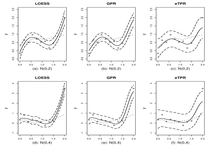
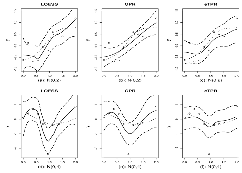
As a motivating example, we generated two data sets with $m=1$ and sample size of $n_{1}=10$ where $x_{1j}$’s are evenly spaced in [0, 1.5] for the first $n_{1}-1$ data points and the remaining point is at 2.0. Thus, this point is a sparse one, meaning it is far away from the other data points in the input space. In addition, we make the data point 2.0 to be an outlier in output space by adding an extra error from either $N(0,2)$ or $N(0,4)$. To fit the simulated data, covariance kernel takes a combination of squared exponential kernel and Mat$\acute{e}$rn kernel (see the detailed discussion in Section 3.2). Prediction curves, the observed data, the true function and their 95% point-wise confidence intervals, are plotted in Figure 1. It shows that the predictions obtained from LOESS and GPR are very similar but the predictions from eTPR shrinks heavily in the area near the data point 2.0, i.e. selective shrinkage occurs. Another example with an outlier in the middle of the interval is presented in Figure D.6 and shows a similar phenomenon. This shows the robustness of eTPR. However, in some other numerical studies, we found that the difference between GPR and eTPR is ignorable. This motivates us to study the eTPR models carefully and comprehensively in both theory and implementation.

Denote the observed data set by $\mbox{{\boldmath${{\mathcal{D}}}$}${}_{n}$}=\{\mbox{{\boldmath${X}$}${}_{i}$},\mbox{{\boldmath${y}$}${}_{i}$},i=1,...,m\}$ where $\mbox{{\boldmath${y}$}${}_{i}$}=(y_{i1},...,y_{in_{i}})^{T}$ and $\mbox{{\boldmath${X}$}${}_{i}$}=(\mbox{{\boldmath${x}$}${}_{i1}$},...,\mbox{{\boldmath${x}$}${}_{in_{i}}$})^{T}$. For a random component $f_{i}(\mbox{\boldmath${u}$})$ at a new point $\mbox{\boldmath${u}$}\in\mathcal{X}$, the best unbiased predictor is $E(f_{i}(\mbox{\boldmath${u}$})|\mbox{{\boldmath${{\mathcal{D}}}$}${}_{n}$}).$ It is called a BLUP if it is linear in {$\mbox{{\boldmath${y}$}${}_{i}$},i=1,...,m$}. Its standard error can be estimated with $Var(f_{i}(\mbox{\boldmath${u}$})|\mbox{{\boldmath${{\mathcal{D}}}$}${}_{n}$}).$ To have an efficient implementation procedure, it is useful to have explicit forms for the predictive distribution $p(f_{i}(\mbox{\boldmath${u}$})|\mbox{{\boldmath${{\mathcal{D}}}$}${}_{n}$}),$ and the first two moments $E(f_{i}(\mbox{\boldmath${u}$})|\mbox{{\boldmath${{\mathcal{D}}}$}${}_{n}$})$ and $Var(f_{i}(\mbox{\boldmath${u}$})|\mbox{{\boldmath${{\mathcal{D}}}$}${}_{n}$})$.

Let $f$ be a real-valued random function such that $f:{\mathcal{X}}\rightarrow R$. In this paper, we extend a Gaussian process to a t-process using the idea in Lee and Nelder (2006):

$$f|r\sim GP(h,rk),~{}~{}~{}~{}r\sim\mathrm{IG}(\nu,\omega),$$

where $GP(h,rk)$ stands for a GP with mean function $h$ and covariance function $rk$, and $\mathrm{IG}(\nu,\omega)$ stands for an inverse gamma distribution. Then, $f$ follows an ETP $f\sim ETP(\nu,\omega,h,k),$ implying that for any collection of points $\mbox{\boldmath${X}$}=(\mbox{{\boldmath${x}$}${}_{1}$},...,\mbox{{\boldmath${x}$}${}_{n}$})^{T},\mbox{{\boldmath${x}$}${}_{i}$}\in{\mathcal{X}}$, we have

$$\mbox{{\boldmath${f}$}${}_{n}$}=f(\mbox{{\boldmath${X}$}$$})=(f(\mbox{{\boldmath${x}$}${}_{1}$}),...,f(\mbox{{\boldmath${x}$}${}_{n}$}))^{T}\sim EMTD(\nu,\omega,\mbox{{\boldmath${h}$}${}_{n}$},\mbox{{\boldmath${K}$}${}_{n}$}),$$

meaning that ${f}$n has an extended multivariate $t$-distribution (EMTD) with the density function,

$$p(z)=|2\pi\omega\mbox{{\boldmath${K}$}${}_{n}$}|^{-1/2}\frac{\Gamma(n/2+\nu)}{\Gamma(\nu)}\left(1+\frac{(z-\mbox{{\boldmath${h}$}${}_{n}$})^{T}\mbox{{\boldmath${K}$}${}_{n}^{-1}$}(z-\mbox{{\boldmath${h}$}${}_{n}$})}{2\omega}\right)^{-(n/2+\nu)},$$

$\mbox{{\boldmath${h}$}${}_{n}$}=(h(\mbox{{\boldmath${x}$}${}_{1}$}),...,h(\mbox{{\boldmath${x}$}${}_{n}$}))^{T}$, $\mbox{{\boldmath${K}$}${}_{n}$}=(k_{ij})_{n\times n}$ and $k_{ij}=k(\mbox{{\boldmath${x}$}${}_{i}$},\mbox{{\boldmath${x}$}${}_{j}$})$ for some mean function $h(\cdot):{\mathcal{X}}\rightarrow R$ and covariance kernel $k(\cdot,\cdot):{\mathcal{X}}\times{\mathcal{X}}\rightarrow R.$

It follows that at any collection of finite points ETP has an analytically representable EMTD density being similar to GP having multivariate normal density. Note that $E(\mbox{{\boldmath${f}$}${}_{n}$})=\mbox{{\boldmath${h}$}${}_{n}$}$ is defined when $\nu>1/2$ and $Cov(\mbox{{\boldmath${f}$}${}_{n}$})=\omega\mbox{{\boldmath${K}$}${}_{n}$}/(\nu-1)$ is defined when $\nu>1$. When $\nu=\omega=\alpha/2$, ${f}$n becomes the multivariate $t$-distribution of Lange et al. (1989). When $\nu=\alpha/2$ and $\omega=\beta/2$, ${f}$n becomes the generalized multivariate $t$-distribution of Arellano-Valle and Bolfarine (1995). For $f\sim ETP(\nu,\omega,0,k)$ it easily obtains that $E(f(\mbox{\boldmath${x}$}))=0,~{}~{}Var(f(\mbox{\boldmath${x}$}))={\omega}k(\mbox{\boldmath${x}$},\mbox{\boldmath${x}$})/{(\nu-1)}$, and

$\displaystyle Skewness(f(\mbox{\boldmath${x}$}))=\frac{E(f^{3}(\mbox{\boldmath${x}$}))}{(E(f^{2}(\mbox{\boldmath${x}$})))^{3/2}}=0,$
$\displaystyle Kurtosis(f(\mbox{\boldmath${x}$}))=\frac{E(f^{4}(\mbox{\boldmath${x}$}))}{(E(f^{2}(\mbox{\boldmath${x}$})))^{2}}=\frac{3}{\nu-2}+3\geq 3\text{ when }\nu>2.$

Thus, we may say that the $ETP(\nu,\omega,0,k)$ has a heavier tail than the $GP(0,k)$.

Proposition 1 Let $f\sim ETP(\nu,\omega,h,k).$

  • (i)

    When $\omega/\nu\rightarrow\lambda$ as $\nu\rightarrow\infty$, we have $\lim_{\nu\rightarrow\infty}ETP(\nu,\omega,h,k)=GP(h,\lambda k).$

  • (ii)

    Let $\mbox{\boldmath${Z}$}\in\mathcal{X}$ be a p$\times 1$ random vector such that $\mbox{\boldmath${Z}$}\sim EMTD(\nu,\omega,\mbox{{\boldmath${\mu}$}${}_{z}$},\mbox{{\boldmath${\Sigma}$}${}_{z}$})$. For a linear system $f(\mbox{\boldmath${x}$})=\mbox{{\boldmath${x}$}${}^{T}$}\mbox{\boldmath${Z}$}$ with $\mbox{\boldmath${x}$}\in\mathcal{X}$, we have $f\sim ETP(\nu,\omega,h,k)$ with $h(\mbox{\boldmath${x}$})=\mbox{{\boldmath${x}$}${}^{T}$}\mbox{{\boldmath${\mu}$}${}_{z}$}$ and $k(\mbox{{\boldmath${x}$}${}_{i}$},\mbox{{\boldmath${x}$}${}_{j}$})=\mbox{{\boldmath${x}$}${}_{i}^{T}$}\mbox{{\boldmath${\Sigma}$}${}_{z}$}\mbox{{\boldmath${x}$}${}_{j}$}$ .

  • (iii)

    Let $\mbox{\boldmath${u}$}\in\mathcal{X}$ be a new data point and $\mbox{{\boldmath${k}$}${}_{u}$}=(k(\mbox{\boldmath${u}$},\mbox{{\boldmath${x}$}${}_{1}$}),...,k(\mbox{\boldmath${u}$},\mbox{{\boldmath${x}$}${}_{n}$}))^{T}.$ Then, $f|\mbox{{\boldmath${f}$}${}_{n}$}\sim ETP(\nu^{\ast},\omega^{\ast},h^{\ast},k^{\ast})$ with $\nu^{\ast}=\nu+n/2,$ $\omega^{\ast}=\omega+n/2$,

    $\displaystyle h^{\ast}(\mbox{\boldmath${u}$})=\mbox{{\boldmath${k}$}${}_{u}^{T}$}\mbox{{\boldmath${K}$}${}_{n}^{{-1}}$}(\mbox{{\boldmath${f}$}${}_{n}$}-\mbox{{\boldmath${h}$}${}_{n}$})+h(\mbox{\boldmath${u}$}),$
    $\displaystyle\mathit{k^{\ast}(\mbox{\boldmath${u}$},\mbox{\boldmath${v}$})}=\frac{{2\omega+(\mbox{{\boldmath${f}$}${}_{n}$}-\mbox{{\boldmath${h}$}${}_{n}$})^{T}\mbox{{\boldmath${K}$}${}_{n}^{{-1}}$}(\mbox{{\boldmath${f}$}${}_{n}$}-\mbox{{\boldmath${h}$}${}_{n}$})}}{{2\omega+n}}\ \left(k(\mbox{\boldmath${u}$},\mbox{\boldmath${v}$})-\mbox{{\boldmath${k}$}${}_{u}^{T}$}\mbox{{\boldmath${K}$}${}_{n}^{{-1}}$}\mbox{{\boldmath${k}$}${}_{v}$}\right),$

    for $\mbox{\boldmath${v}$}\in\mathcal{X}$.

Even if the mean and covariance functions of $f\sim ETP(\nu,\omega,h,k)$ can not be defined when $\nu<0.5$, from Proposition 1(iii), the mean and covariance functions of the conditional process $f|\mbox{{\boldmath${f}$}${}_{n}$}$ do always exist if $n\geq 2$. Also from Proposition 1(iii), the conditional process $ETP(\nu^{\ast},\omega^{\ast},h^{\ast},k^{\ast})$ converges to a GP, as either $\nu$ or $n$ tends to $\infty$. Thus, if the sample size $n$ is large enough, the ETP behaves like a GP.

For a new point ${u}$, we have $f(\mbox{\boldmath${u}$})|\mbox{{\boldmath${f}$}${}_{n}$}\sim EMTD(\nu^{\ast},\omega^{\ast},h^{\ast}(\mbox{\boldmath${u}$}),k^{\ast}(\mbox{\boldmath${u}$},\mbox{\boldmath${u}$}))$, where

$\displaystyle h^{\ast}(\mbox{\boldmath${u}$})=E(f(\mbox{\boldmath${u}$})|\mbox{{\boldmath${f}$}${}_{n}$})=\mbox{{\boldmath${k}$}${}_{u}^{T}$}\mbox{{\boldmath${K}$}${}_{n}^{{-1}}$}(\mbox{{\boldmath${f}$}${}_{n}$}-\mbox{{\boldmath${h}$}${}_{n}$})+h(\mbox{\boldmath${u}$}),$
$\displaystyle Var(f(\mbox{\boldmath${u}$})|\mbox{{\boldmath${f}$}${}_{n}$})=\frac{\omega^{\ast}}{\nu^{\ast}-1}k^{\ast}(\mbox{\boldmath${u}$},\mbox{\boldmath${u}$})=s~{}\{k(\mbox{\boldmath${u}$},\mbox{\boldmath${u}$})-\mbox{{\boldmath${k}$}${}_{u}^{T}$}\mbox{{\boldmath${K}$}${}_{n}^{{-1}}$}\mbox{{\boldmath${k}$}${}_{u}$}\},$

and $s=({2\omega+(\mbox{{\boldmath${f}$}${}_{n}$}-\mbox{{\boldmath${h}$}${}_{n}$})^{T}\mbox{{\boldmath${K}$}${}_{n}^{{-1}}$}(\mbox{{\boldmath${f}$}${}_{n}$}-\mbox{{\boldmath${h}$}${}_{n}$})})/({2\nu+n-2})$. Note that from Lemma 2(iv) in Appendix A, $s=E(r|\mbox{{\boldmath${f}$}${}_{n}$})$.

Under various combinations of $\nu$ and $\omega$, the ETP generates various $t$-processes proposed in the literature. For example, $ETP(\alpha/2,\alpha/2-1,h,k)$ is the $t$-process of Shah et al. (2014). They showed that if covariance function ${\Sigma}$ follows an inverse Wishart process with parameter $\alpha=2\nu$ and kernel function $k$, and $f|\mbox{\boldmath${\Sigma}$}\sim GP(h,(\alpha-2)\mbox{\boldmath${\Sigma}$})$, then $f$ has an extended $t$-process $ETP(\alpha/2,\alpha/2-1,h,k)$. $ETP(\alpha/2,\alpha/2,h,k)$ is the Student’s $t$-process of Rasmussen and Williams (2006) and $ETP(\nu,1/2,h,k)$ is the model discussed in Zhang and Yeung (2010).

3 eTPR models

For the process regression model (2), this paper assumes that $(f_{i},\epsilon_{i}),i=1,...,m$, are independent, and $f_{i}$ and $\epsilon_{i}$ have a joint ETP process,

$$\left(\begin{array}[]{c}f_{i}\\ \epsilon_{i}\end{array}\right)\sim ETP\left(\nu,\omega,\left(\begin{array}[]{c}h_{i}\\ 0\end{array}\right),\left(\begin{array}[]{cc}k_{i}&0\\ 0&k_{\epsilon}\end{array}\right)\right),$$ (3)

where $h_{i}$ and $k_{i}$ are mean and kernel functions, $k_{\epsilon}(\mbox{\boldmath${u}$},\mbox{\boldmath${v}$})=\phi I(\mbox{\boldmath${u}$}=\mbox{\boldmath${v}$})$ and $I(\cdot)$ is an indicator function. We can construct the ETP (3) hierarchically as

$$\left(\begin{array}[]{c}f_{i}\\ \epsilon_{i}\end{array}\right)\Big{|}r_{i}\sim GP\left(\left(\begin{array}[]{c}h_{i}\\ 0\end{array}\right),r_{i}\left(\begin{array}[]{cc}k_{i}&0\\ 0&k_{\epsilon}\end{array}\right)\right){\mbox{~{} and~{} }}r_{i}\sim\mathrm{{IG}(\nu,\omega)},$$

which implies that $f_{i}+\epsilon_{i}|r_{i}\sim GP(h_{i},r_{i}(k_{i}+k_{\epsilon}))$ and $r_{i}\sim\mathrm{{IG}(\nu,\omega)}$ results in $y_{i}\sim ETP(\nu,\omega,h_{i},k_{i}+k_{\epsilon}).$ We call the above model as an extended t-process regression model (eTPR). Hence, additivity property of the GPR and many other properties hold conditionally and marginally for the eTPR. When $r_{i}=1$, the eTPR model becomes a GPR model. Without loss of generality, let $n_{1}=\cdots=n_{m}=n$. For observed data $\mbox{{\boldmath${{\mathcal{D}}}$}${}_{n}$}=\{\mbox{{\boldmath${X}$}${}_{i}$},\mbox{{\boldmath${y}$}${}_{i}$},i=1,...,m\}$ with $\mbox{{\boldmath${y}$}${}_{i}$}=(y_{i1},...,y_{in})^{T}$ and $\mbox{{\boldmath${X}$}${}_{i}$}=(\mbox{{\boldmath${x}$}${}_{i1}$},...,\mbox{{\boldmath${x}$}${}_{in}$})^{T}$, the model can be expressed as

$\displaystyle f_{i}(\mbox{{\boldmath${X}$}${}_{i}$})|\mbox{{\boldmath${X}$}${}_{i}$}\sim EMTD(\nu,\omega,\mbox{{\boldmath${h}$}${}_{in}$},\mbox{{\boldmath${K}$}${}_{in}$}),$
$\displaystyle\mbox{{\boldmath${y}$}${}_{i}$}|f_{i},\mbox{{\boldmath${X}$}${}_{i}$}\sim EMTD(\nu,\omega,f_{i}(\mbox{{\boldmath${X}$}${}_{i}$}),\phi\mbox{{\boldmath${I}$}${}_{n}$}),$
$\displaystyle\mbox{{\boldmath${y}$}${}_{i}$}|\mbox{{\boldmath${X}$}${}_{i}$}\sim EMTD(\nu,\omega,\mbox{{\boldmath${h}$}${}_{in}$},\mbox{{\boldmath${\Sigma}$}${}_{in}$}),$

where $\mbox{{\boldmath${h}$}${}_{in}$}=(h_{i}(\mbox{{\boldmath${x}$}${}_{i1}$}),...,h_{i}(\mbox{{\boldmath${x}$}${}_{in}$}))^{T}$, $\mbox{{\boldmath${K}$}${}_{in}$}=(k_{ijl})_{n\times n}$, $k_{ijl}=k_{i}(\mbox{{\boldmath${x}$}${}_{ij}$},\mbox{{\boldmath${x}$}${}_{il}$})$, and $\mbox{{\boldmath${\Sigma}$}${}_{in}$}=\mbox{{\boldmath${K}$}${}_{in}$}+\phi\mbox{{\boldmath${I}$}${}_{n}$}$.

Consider a linear mixed model

$$y_{1j}=\mbox{{\boldmath${w}$}${}_{j}^{T}$}\mbox{\boldmath${\delta}$}+\mbox{{\boldmath${v}$}${}_{j}^{T}$}\mbox{\boldmath${b}$}+\epsilon_{1j},~{}~{}j=1,...,n,$$

where ${w}$j is the design matrix for fixed effects ${\delta}$, ${v}$j is the design matrix for random effect $\mbox{\boldmath${b}$}\thicksim N(0,\theta\mbox{{\boldmath${I}$}${}_{p}$})$ and $\epsilon_{1j}\thicksim N(0,\phi)$ is a white noise. Suppose that $\mbox{{\boldmath${X}$}${}_{1}$}=(\mbox{{\boldmath${W}$}${}_{n}$},\mbox{{\boldmath${V}$}${}_{n}$})$, $\ f_{1}(\mbox{{\boldmath${X}$}${}_{1}$})=\mbox{{\boldmath${W}$}${}_{n}^{T}$}\mbox{\boldmath${\delta}$}+\mbox{{\boldmath${V}$}${}_{n}^{T}$}\mbox{\boldmath${b}$}$, $\mbox{{\boldmath${h}$}${}_{1n}$}=\mbox{{\boldmath${W}$}${}_{n}^{T}$}\mbox{\boldmath${\delta}$}$ and $\mbox{{\boldmath${K}$}${}_{1n}$}=\theta\mbox{{\boldmath${V}$}${}_{n}$}\mbox{{\boldmath${V}$}${}_{n}^{T}$}$ with $\mbox{{\boldmath${W}$}${}_{n}$}=(\mbox{{\boldmath${w}$}${}_{1}$},...,\mbox{{\boldmath${w}$}${}_{n}$})^{T}$ and $\mbox{{\boldmath${V}$}${}_{n}$}=(\mbox{{\boldmath${v}$}${}_{1}$},...,\mbox{{\boldmath${v}$}${}_{n}$})^{T}$. Then, the linear mixed model becomes the functional regression model with

$\displaystyle f_{1}(\mbox{{\boldmath${X}$}${}_{1}$})|\mbox{{\boldmath${X}$}${}_{1}$}=\mbox{{\boldmath${W}$}${}_{n}^{T}$}\mbox{\boldmath${\delta}$}+\mbox{{\boldmath${V}$}${}_{n}^{T}$}\mbox{\boldmath${b}$}|\mbox{{\boldmath${X}$}${}_{1}$}\sim N(\mbox{{\boldmath${W}$}${}_{n}^{T}$}\mbox{\boldmath${\delta}$},\mbox{{\boldmath${K}$}${}_{1n}$}),$
$\displaystyle\mbox{{\boldmath${y}$}${}_{1}$}|f_{1},\mbox{{\boldmath${X}$}${}_{1}$}=\mbox{{\boldmath${y}$}${}_{1}$}|\mbox{\boldmath${b}$},\mbox{{\boldmath${X}$}${}_{1}$}\sim N(\mbox{{\boldmath${W}$}${}_{n}^{T}$}\mbox{\boldmath${\delta}$}+\mbox{{\boldmath${V}$}${}_{n}^{T}$}\mbox{\boldmath${b}$},\phi\mbox{{\boldmath${I}$}${}_{n}$}),$
$\displaystyle\mbox{{\boldmath${y}$}${}_{1}$}|\mbox{{\boldmath${X}$}${}_{1}$}\sim N(\mbox{{\boldmath${W}$}${}_{n}^{T}$}\mbox{\boldmath${\delta}$},\mbox{{\boldmath${\Sigma}$}${}_{1n}$}).$

This shows that the eTPR model extends the conventional normal linear mixed models to a nonlinear concurrent functional regression. Contrary to LOESS, this also shows that the eTPR method can produce a regression function, easily represented by a mathematical formula.

3.1 Parameter estimation

So far we have assumed that the covariance kernel $k_{i}(\cdot,\cdot)$ is given. To fit the eTPR model, we need to choose $k_{i}(\cdot,\cdot)$. A way is to estimate the covariance kernel nonparametrically; see e.g. Hall et al. (2008). However, this method is very difficult to be applied to problems with multivariate covariates. Thus, we choose a covariance kernel from a covariance function family such as a squared exponential kernel and Matérn class kernel.

Let $\mbox{\boldmath${\beta}$}=(\phi,\mbox{\boldmath${\theta}$}_{1},...,\mbox{\boldmath${\theta}$}_{m})$, where $\phi$ is a parameter for $\epsilon(\mbox{\boldmath${x}$})$ and $\mbox{\boldmath${\theta}$}_{i}$ are those for $f_{i}(\mbox{{\boldmath${x}$}})$ (parameters involved in the kernel $k_{i}$), $i=1,...,m$. Because $\mbox{{\boldmath${y}$}${}_{i}$}|\mbox{{\boldmath${X}$}${}_{i}$}\sim EMTD(\nu,\omega,0,\mbox{{\boldmath${\Sigma}$}${}_{in}$})$, the maximum likelihood (ML) estimator for ${\beta}$ can be obtained by solving

$$\sum_{i=1}^{m}\frac{\partial\log p{{}_{\beta}(\mbox{{\boldmath${y}$}${}_{i}$}|\mbox{{\boldmath${X}$}${}_{i}$})}}{\partial\beta_{k}}=\frac{1}{2}\sum_{i=1}^{m}Tr\left(\Big{(}s_{1i}\mbox{\boldmath${\alpha}_{i}$}\mbox{{\boldmath${\alpha}_{i}$}${}^{T}$}-\mbox{{\boldmath${{\Sigma}}$}${}_{in}^{-1}$}\Big{)}\frac{\partial\mbox{{\boldmath${{\Sigma}}$}${}_{in}$}}{\partial\beta_{k}}\right)=0,$$ (4)

where $\beta_{k}$ is the $k$th element of ${\beta}$, $\mbox{\boldmath${\alpha}_{i}$}=\mbox{{\boldmath${{\Sigma}}$}${}_{in}^{-1}$}\mbox{{\boldmath${y}$}${}_{i}$}$, $s_{1i}=({n+2\nu})/({2\omega+\mbox{{\boldmath${y}$}${}_{i}^{T}$}\mbox{{\boldmath${{\Sigma}}$}${}_{in}^{-1}$}\mbox{{\boldmath${y}$}${}_{i}$}})$, and

$$p_{\beta}(\mbox{{\boldmath${y}$}${}_{i}$}|\mbox{{\boldmath${X}$}${}_{i}$})=|2\pi\omega\mbox{{\boldmath${{\Sigma}}$}${}_{in}$}|^{-1/2}\frac{\Gamma(n/2+\nu)}{\Gamma(\nu)}\left(1+\frac{\mbox{{\boldmath${y}$}${}_{i}^{T}$}\mbox{{\boldmath${\Sigma}$}${}_{in}^{-1}$}\mbox{{\boldmath${y}$}${}_{i}$}}{2\omega}\right)^{-(n/2+\nu)}.$$ (5)

Score equations for GPR models are the ML estimating equations above with $\nu=\infty$ and $s_{1i}=1$. Thus, a parameter estimation for the eTPR models can be obtained by a modification of the existing procedures for the GPR models.

From the hierarchical construction of ETP with $m=1$, there is only one single random effect $r_{1}$, so that $r_{1}$ is not estimable, confounded with parameters in covariance matrix. This means that $\nu$ and $\omega$ are not estimable. Following Lee and Nelder (2006), we set $\omega=\nu-1$. Thus $Var(f)=\omega k/(\nu-1)=k,$ i.e. the variance does not depend upon $\nu$ and $\omega.$ When $f\sim GP(h,k)$ $Var(f)=k.$ Under this setting, the first two moments of GP and ETP have the same form allowing a common interpretation of parameters for the variance for both GPR and eTPR models. Zellener (1976) also noted that $\nu$ cannot be estimated with a single realization. In multivariate t-distribution, Lange et al. (1989) proposed to use $\nu=2$. Zellener (1976) suggested that $\nu$ can be chosen according to investigator’s knowledge of robustness of regression error distribution. As $\nu\rightarrow\infty$, ETP tends to GP. When robustness property is an important issue, a smaller $\nu$ is preferred. We tried various values for $v$ and find that $v=1.05$ works well. From now on, when $m=1$ we set $v=1.05$ and $\omega=\nu-1=0.05.$

When $m>1$, the eTPR model (3) includes $m$ random effects $r_{i}$, $i=1,...,m$. Thus, $\nu$ can be estimted. We have a score equation for $\nu$ as follows,

$\displaystyle\sum_{i=1}^{m}\frac{\partial\log p{{}_{\beta}(\mbox{{\boldmath${y}$}${}_{i}$}|\mbox{{\boldmath${X}$}${}_{i}$})}}{\partial\nu}=-\frac{1}{2}\sum_{i=1}^{m}\Big{\{}\frac{n}{\nu-1}+2\log\Big{(}1+\frac{\mbox{{\boldmath${y}$}${}_{i}^{T}$}\mbox{{\boldmath${\Sigma}$}${}_{in}^{-1}$}\mbox{{\boldmath${y}$}${}_{i}$}}{2(\nu-1)}\Big{)}$
$\displaystyle-\frac{(n+2\nu)\mbox{{\boldmath${y}$}${}_{i}^{T}$}\mbox{{\boldmath${\Sigma}$}${}_{in}^{-1}$}\mbox{{\boldmath${y}$}${}_{i}$}}{2(\nu-1)^{2}+(\nu-1)\mbox{{\boldmath${y}$}${}_{i}^{T}$}\mbox{{\boldmath${\Sigma}$}${}_{in}^{-1}$}\mbox{{\boldmath${y}$}${}_{i}$}}-2\psi(\frac{n}{2}+\nu)+2\psi(\nu)\Big{\}}=0,$

where $\psi(\cdot)$ is a digamma function satisfying $\psi(t+1)=\psi(t)+1/t$ for $t\in R$.

We assume $h_{i}(\mbox{\boldmath${u}$})=0$ as in GPR models. It is straightforward to extend the proposed method to mean function with general form.

3.2 Predictive distribution

Since

$$\left(\begin{array}[]{c}f_{i}(\mbox{{\boldmath${X}$}${}_{i}$})\\ \mbox{{\boldmath${y}$}${}_{i}$}\end{array}\right)\Bigg{|}\mbox{{\boldmath${X}$}${}_{i}$}\sim EMTD\left(\nu,\nu-1,0,\left(\begin{array}[]{cc}\mbox{{\boldmath${K}$}${}_{in}$}&\mbox{{\boldmath${K}$}${}_{in}$}\\ \mbox{{\boldmath${K}$}${}_{in}$}&\mbox{{\boldmath${\Sigma}$}${}_{in}$}\end{array}\right)\right),$$

from Lemma 2(iii) in Appendix A we have $f_{i}(\mbox{{\boldmath${X}$}${}_{i}$})|\mbox{{\boldmath${\cal D}$}${}_{n}$}\thicksim EMTD(n/2+\nu,n/2+\nu-1,\mbox{{\boldmath${\mu}$}${}_{in}$},\mbox{{\boldmath${C}$}${}_{in}$}),$ with

$\displaystyle\mbox{{\boldmath${\mu}$}${}_{in}$}=E(f_{i}(\mbox{{\boldmath${X}$}${}_{i}$})|\mbox{{\boldmath${\cal D}$}${}_{n}$})=\mbox{{\boldmath${K}$}${}_{in}$}\mbox{{\boldmath${\Sigma}$}${}_{in}^{-1}$}\mbox{{\boldmath${y}$}${}_{i}$},$
$\displaystyle\mbox{{\boldmath${C}$}${}_{in}$}=Cov(f_{i}(\mbox{{\boldmath${X}$}${}_{i}$})|\mbox{{\boldmath${\cal D}$}${}_{n}$})=s_{0i}\phi\mbox{{\boldmath${K}$}${}_{in}$}\mbox{{\boldmath${\Sigma}$}${}_{in}^{-1}$},$
$\displaystyle s_{0i}=E(r_{i}|\mbox{{\boldmath${\cal D}$}${}_{n}$})=\frac{\mbox{{\boldmath${y}$}${}_{i}^{T}$}\mbox{{\boldmath${\Sigma}$}${}_{in}^{-1}$}\mbox{{\boldmath${y}$}${}_{i}$}+2(\nu-1)}{n+2(\nu-1)}.$

Thus, given $\mbox{\boldmath${\beta}$},$ $\hat{\mbox{\boldmath${f}$}}_{in}=E(f_{i}(\mbox{{\boldmath${X}$}${}_{i}$})|\mbox{{\boldmath${\cal D}$}${}_{n}$})$ is linear in $\mbox{{\boldmath${y}$}${}_{i}$},$ i.e. the BLUP for $f_{i}(\mbox{{\boldmath${X}$}${}_{i}$}),$ which is an extension of the BLUP in linear mixed models to eTPR models. This BLUP has a form independent of $\nu$, so that it is also the BLUP under GPR models. However, the conditional variance depends upon $\nu$.

For a given new data point ${u}$, we have

$$\left(\begin{array}[]{c}\mbox{{\boldmath${y}$}${}_{i}$}\\ f_{i}(\mbox{\boldmath${u}$})\end{array}\right)\Bigg{|}\mbox{{\boldmath${X}$}${}_{i}$}\sim EMTD\left(\nu,\nu-1,0,\left(\begin{array}[]{cc}\mbox{{\boldmath${\Sigma}$}${}_{in}$}&\mbox{{\boldmath${k}$}${}_{iu}$}\\ \mbox{{\boldmath${k}$}${}_{iu}^{T}$}&k_{i}(\mbox{\boldmath${u}$},\mbox{\boldmath${u}$})\end{array}\right)\right),$$

where $\mbox{{\boldmath${k}$}${}_{iu}$}=(k_{i}(\mbox{{\boldmath${x}$}${}_{i1}$},\mbox{\boldmath${u}$}),\cdots,k_{i}(\mbox{{\boldmath${x}$}${}_{in}$},\mbox{\boldmath${u}$}))^{T}$. By Lemma 2(iii), the predictive distribution $p(f_{i}(\mbox{\boldmath${u}$})|\mbox{{\boldmath${\mathcal{D}}$}${}_{n}$})$ is $EMTD(n/2+\nu,n/2+\nu-1,\mu_{in}^{\ast},\sigma_{in}^{\ast}),$ where

$\displaystyle\mu_{in}^{\ast}=E(f_{i}(\mbox{\boldmath${u}$})|\mbox{{\boldmath${\mathcal{D}}$}${}_{n}$})=\mbox{{\boldmath${k}$}${}_{iu}^{T}$}\mbox{{\boldmath${{\Sigma}}$}${}_{in}^{{-1}}$}\mbox{{\boldmath${y}$}${}_{i}$},$ (6)
$\displaystyle\sigma_{in}^{\ast}=Var(f_{i}(\mbox{\boldmath${u}$})|\mbox{{\boldmath${\mathcal{D}}$}${}_{n}$})=s_{0i}\Big{(}k_{i}(\mbox{\boldmath${u}$},\mbox{\boldmath${u}$})-\mbox{{\boldmath${k}$}${}_{iu}^{T}$}\mbox{{\boldmath${{\Sigma}}$}${}_{in}^{-1}$}\mbox{{\boldmath${k}$}${}_{iu}$}\Big{)}.$ (7)

Furthermore, from Proposition 1(iii), ${\ f_{i}|\mbox{{\boldmath${\mathcal{D}}$}${}_{n}$}}\sim ETP{(n/2+\nu,n/2+\nu-1,\ h_{i}^{\ast},k_{i}^{\ast}),\ }$ where $h_{i}^{\ast}(\mbox{\boldmath${u}$})=\mu^{*}_{in}$ and $k_{i}^{\ast}(\mbox{\boldmath${u}$},\mbox{\boldmath${v}$})=s_{0i}\Big{(}k_{i}(\mbox{\boldmath${u}$},\mbox{\boldmath${v}$})-k_{iu}^{T}\mbox{{\boldmath${{\Sigma}}$}${}_{in}^{-1}$}k_{iv}\Big{)}.$ From Lemma 2(iii), we also have $y_{i}(\mbox{\boldmath${u}$})|\mbox{{\boldmath${\mathcal{D}}$}${}_{n}$}\thicksim EMTD(n/2+\nu,n/2+\nu-1,\mu_{in}^{\ast},\sigma_{in}^{\ast}+s_{0i}\phi)$ with $E(y_{i}(\mbox{\boldmath${u}$})|\mbox{{\boldmath${\mathcal{D}}$}${}_{n}$})=\mu_{in}^{\ast}$ and $Var(y_{i}(\mbox{\boldmath${u}$})|\mbox{{\boldmath${\mathcal{D}}$}${}_{n}$})=\sigma_{in}^{\ast}+s_{0i}\phi$. Consequently, this conditional predictive process can be used to construct prediction $\hat{y}_{i}(\mbox{\boldmath${u}$})=E(y_{i}(\mbox{\boldmath${u}$})|\mbox{{\boldmath${\mathcal{D}}$}${}_{n}$})=$ $E(f_{i}(\mbox{\boldmath${u}$})|\mbox{{\boldmath${\mathcal{D}}$}${}_{n}$})$ of the unobserved response $y_{i}(\mbox{\boldmath${u}$})$ at $\mbox{\boldmath${x}$}=\mbox{\boldmath${u}$}$ and its standard error can be formed using the predictive variance, given by $\sigma_{in}^{\ast}+s_{0i}\phi$. The proof is given in Appendix B.2. The predictive variance for $\hat{f}_{i}(\mbox{\boldmath${u}$})=\mu_{in}^{*}$ in (7) differs from that for $\hat{y}_{i}(\mbox{\boldmath${u}$}).$

Shah et al. (2014) discussed the case of $m=1$ and stated that “both the predictive mean and the predictive covariance of a TP will differ from that of a GP after learning kernel hyperparameters”. Their statement is only partly true when $m=1$. However we show that predictive means and variances from eTPR and GPR models always differ when $m>1$. We consider five commonly used covariance functions here (Rasmussen and Williams, 2006; Shi and Choi, 2011): squared exponential kernel ($k_{se}$), non-stationary linear kernel ($k_{lin}$), von Mises-inspired kernel ($k_{vm}$), rational quadratic kernel ($k_{rq}$) and Mat$\acute{e}$rn kernel ($k_{m}$) (see the details in Appendix B.2).

Proposition 2 (The model with $m=1$)

  • (i)

    Under the kernel functions $k_{se}$, $k_{lin}$ and $k_{vm}$, the predictions of $f_{1}(\mbox{{\boldmath${X}$}${}_{1}$})$ and $f_{1}(\mbox{\boldmath${u}$})$ from eTPR models are exactly the same as those from GPR models.

  • (ii)

    Under $k_{rq}$ and $k_{m}$, eTPR and GPR models produce different predictions. And the predictive standard error from the eTPR model increases if the model does not fit the responses well while that under the GPR model does not depend upon the model fit.

Proposition 3 (The model with $m>1$)
When $m>1$, $\nu$ can be estimated. The eTPR and GPR models under all the five kernel functions discussed above have different values of predictions and predictive variances. The predictive variance under the eTPR model decreases if the model fits the responses ${y}$i better while that under the GPR model is still independent of the model fit.

The proofs of Propositions 2 and 3 are given in Appendix B.2. This paper takes two combinations of $k_{se}+k_{lin}$ and $k_{se}+k_{m}$ in simulation studies. For the first combination $k_{se}+k_{lin}$, eTPR and GPR models with $m=1$ have the exactly same predictions, but the eTPR has a slightly larger values of predictive variance than the GPR. For the second case, both predictions and predictive variances are different.

Random-effect models consist with three objects, namely the data ${\mathcal{D}}$n, unobservables (random effects) and parameters (fixed unknowns) $\mbox{\boldmath${\beta}$}.$ For inferences of such models, Lee and Nelder (1996) proposed the use of the h-likelihood. Lee and Kim (2015) showed that inferences about unobservables allow both Bayesian and frequentist interpretations. In this paper, we see that the eTPR model is an extension of random-effect models. Thus, we may view the functional regression model (2) either as a Bayesian model, where a GP or an ETP as a prior, or as a frequentist model where a latent process such as GP and ETP is used to fit unknown function $f_{01}$ in a functional space (Chapter 9, Lee et al. (2006)). With the predictive distribution above, we may form both Bayesian credible and frequentist confidence intervals. Estimation procedures in Section 3.1 can be viewed as an empirical Bayesian method with a uniform prior on $\mbox{\boldmath${\beta}$}.$ In frequentist (or Bayesian) approach, (5) is a marginal likelihood for fixed (or hyper) parameters.

4 Robustness and information consistency

4.1 Robust properties

The eTPR models give robust estimates of parameters and the unknown regression function compared to the GPR models. Even with $m=1$, under some kernel functions the eTPR models are more robust against outliers in the output space than the GPR models.

Let $\hat{f}_{iT}(\mbox{\boldmath${u}$})=\hat{\mu}_{in}^{\ast}=\mu_{in}^{*}|_{\mbox{\boldmath${\beta}$}=\hat{\mbox{\boldmath${\beta}$}}}$ and $V_{iT}=\hat{{\sigma}}_{in}^{\ast}={\sigma}_{in}^{*}|_{\mbox{\boldmath${\beta}$}=\hat{\mbox{\boldmath${\beta}$}}}$ be the predictive mean and variance for $f_{i}(\mbox{\boldmath${u}$})$, under the eTPR model. And let $\hat{f}_{iG}(\mbox{\boldmath${u}$})$ and $V_{iG}$ be those under the GPR model with $s_{0i}=1$. Let $M_{iT}=(\hat{f}_{iT}(\mbox{\boldmath${u}$})-f_{i0}(\mbox{\boldmath${u}$}))/\sqrt{V_{iT}}$ and $M_{iG}=(\hat{f}_{iG}(\mbox{\boldmath${u}$})-f_{0i}(\mbox{\boldmath${u}$}))/\sqrt{V_{iG}}$ be two student t-type statistics for a null hypothesis $f_{i}(\mbox{\boldmath${u}$})=f_{i0}(\mbox{\boldmath${u}$})$. Under a bounded kernel function, if $y_{ij}\rightarrow\infty$ for some $j$, $M_{iG}\rightarrow\infty$, while $M_{iT}$ remains bounded. Therefore, $M_{iT}$ for eTPR is more robust against outliers in output space compared to that for GPR. This property still holds for ML estimators.

Proposition 4 If kernel functions $k_{i}$, $i=1,\cdots,m$, are bounded, continuous and differentiable on ${\theta}$i, then for given $\nu$, the ML estimator $\hat{\mbox{\boldmath${\beta}$}}$ from the eTPR has bound influence function, while that from the GPR does not.

4.2 Information Consistency

Let $p_{\phi_{0}}(\mbox{{\boldmath${y}$}${}_{i}$}|f_{0i},\mbox{{\boldmath${X}$}${}_{i}$})$ be the density function to generate the data ${y}$i given ${X}$i under the true model (1), where $f_{0i}$ is the true underlying function of $f_{i}$. Let $p_{\theta_{i}}(f)$ be a measure of random process $f$ on space ${\mathcal{F}}=\{f(\cdot):\mathcal{X}\rightarrow R\}$. Let

$$p_{\phi,\theta_{i}}(\mbox{{\boldmath${y}$}${}_{i}$}|\mbox{{\boldmath${X}$}${}_{i}$})=\int_{{\mathcal{F}}}p_{\phi}(\mbox{{\boldmath${y}$}${}_{i}$}|f,\mbox{{\boldmath${X}$}${}_{i}$})dp_{\theta_{i}}(f),$$

be the density function to generate the data ${y}$i given ${X}$i under the assumed eTPR model (3). Thus, the assumed model (3) is not the same as the true underlying model (1). Here $\phi$ is the common in both models and $\phi_{0}$ is the true value of $\phi$. Let $p_{\phi_{0},\hat{\theta}_{i}}(\mbox{{\boldmath${y}$}${}_{i}$}|\mbox{{\boldmath${X}$}${}_{i}$})$ be the estimated density function under the eTPR model. Denote $D[p_{1},p_{2}]=\int(\log{p_{1}}-\log{p_{2}})dp_{1}$ by the Kullback-Leibler distance between two densities $p_{1}$ and $p_{2}$. Then, for fixed $m$, we have the following proposition.

Proposition 5 Under the appropriate conditions in Lemma 3 and condition (A) of Appendix C, we have for $i=1,\cdots,m$,

$$\frac{1}{n}E_{\mbox{{\boldmath${X}$}${}_{i}$}}(D[p_{\phi_{0}}(\mbox{{\boldmath${y}$}${}_{i}$}|f_{0i},\mbox{{\boldmath${X}$}${}_{i}$}),p_{\phi_{0},\hat{\theta}_{i}}(\mbox{{\boldmath${y}$}${}_{i}$}|\mbox{{\boldmath${X}$}${}_{i}$})])\longrightarrow 0,{\mbox{as}}~{}~{}n\rightarrow\infty,$$

where the expectation is taken over the distribution of ${X}$i.

From Proposition 5, the Kullback-Leibler distance between two density functions for $\mbox{{\boldmath${y}$}${}_{i}$}|\mbox{{\boldmath${X}$}${}_{i}$}$ from the true and the assumed models becomes zero, asymptotically. Let $\mbox{{\boldmath${y}$}${}_{il}$}=(y_{i1},...,y_{il})^{T}$ and $\mbox{{\boldmath${X}$}${}_{il}$}=(\mbox{{\boldmath${x}$}${}_{i1}$},...,\mbox{{\boldmath${x}$}${}_{il}$})^{T}$, $l=1,...,n$. In Appendix C, we show that

$$p_{\phi_{0},\theta_{i}}(\mbox{{\boldmath${y}$}${}_{i}$}|\mbox{{\boldmath${X}$}${}_{i}$})=\prod_{l=1}^{n}p_{\phi_{0},\theta_{i}}(y_{il}|\mbox{{\boldmath${X}$}${}_{il}$},\mbox{{\boldmath${y}$}${}_{i(l-1)}$}),$$ (8)

where

$\displaystyle p_{\phi_{0},\theta_{i}}(y_{il}|\mbox{{\boldmath${X}$}${}_{il}$},\mbox{{\boldmath${y}$}${}_{i(l-1)}$})=\int_{{\mathcal{F}}}p_{\phi_{0}}(y_{il}|f,\mbox{{\boldmath${X}$}${}_{il}$},\mbox{{\boldmath${y}$}${}_{i(l-1)}$})dp_{\theta_{i}}(f|\mbox{{\boldmath${X}$}${}_{il}$},\mbox{{\boldmath${y}$}${}_{i(l-1)}$}),$
$\displaystyle p_{\theta_{i}}(f|\mbox{{\boldmath${X}$}${}_{il}$},\mbox{{\boldmath${y}$}${}_{i(l-1)}$})=\frac{p_{\phi_{0}}(\mbox{{\boldmath${y}$}${}_{i(l-1)}$}|f,\mbox{{\boldmath${X}$}${}_{i(l-1)}$})p_{\theta_{i}}(f)}{\int_{{\mathcal{F}}}p_{\phi_{0}}(\mbox{{\boldmath${y}$}${}_{i(l-1)}$}|f^{\prime},\mbox{{\boldmath${X}$}${}_{i(l-1)}$})dp_{\theta_{i}}(f^{\prime})}.$

Under the true model (1), similarly to (8), we have

$$p_{\phi_{0}}(\mbox{{\boldmath${y}$}${}_{i}$}|f_{0i},\mbox{{\boldmath${X}$}${}_{i}$})=\prod_{l=1}^{n}p_{\phi_{0}}(y_{il}|f_{0i},\mbox{{\boldmath${X}$}${}_{il}$},\mbox{{\boldmath${y}$}${}_{i(l-1)}$}).$$

Seeger et al. (2008) called $p_{\phi_{0}}(y_{il}|f_{0i},\mbox{{\boldmath${X}$}${}_{il}$},\mbox{{\boldmath${y}$}${}_{i(l-1)}$})$ and $p_{\phi_{0},\hat{\theta}_{i}}(y_{il}|\mbox{{\boldmath${X}$}${}_{il}$},\mbox{{\boldmath${y}$}${}_{i(l-1)}$})$ Bayesian prediction strategies. We show that

$$D[p_{\phi_{0}}(\mbox{{\boldmath${y}$}${}_{i}$}|f_{0i},\mbox{{\boldmath${X}$}${}_{i}$}),p_{\phi_{0},\hat{\theta}_{i}}(\mbox{{\boldmath${y}$}${}_{i}$}|\mbox{{\boldmath${X}$}${}_{i}$})]=\int\sum_{l=1}^{n}Q(y_{il}|\mbox{{\boldmath${X}$}${}_{il}$},\mbox{{\boldmath${y}$}${}_{i(l-1)}$})p_{\phi_{0}}(\mbox{{\boldmath${y}$}${}_{i}$}|f_{0i},\mbox{{\boldmath${X}$}${}_{i}$})d\mbox{{\boldmath${y}$}${}_{i}$},$$

where $Q(y_{il}|\mbox{{\boldmath${X}$}${}_{il}$},\mbox{{\boldmath${y}$}${}_{i(l-1)}$})=\log\{p_{\phi_{0}}(y_{il}|f_{0i},\mbox{{\boldmath${X}$}${}_{il}$},\mbox{{\boldmath${y}$}${}_{i(l-1)}$})/p_{\phi_{0},\hat{\theta}_{i}}(y_{il}|\mbox{{\boldmath${X}$}${}_{il}$},\mbox{{\boldmath${y}$}${}_{i(l-1)}$})\}$ is a loss function and $\sum_{l=1}^{n}Q(y_{il}|\mbox{{\boldmath${X}$}${}_{il}$},\mbox{{\boldmath${y}$}${}_{i(l-1)}$})$ is called cumulative loss. Under the GPR model, Seeger et al. (2008) and Wang and Shi (2014) proved information consistency, interpreted it as the average of cumulative loss $\sum_{l=1}^{n}Q(y_{il}|\mbox{{\boldmath${X}$}${}_{il}$},\mbox{{\boldmath${y}$}${}_{i(l-1)}$})/n$ tending to zero asymptotically. In this paper, we show this property for the robust BLUPs. Consequently, the frequentist BLUP procedure is consistent with the Bayesian strategy in terms of average risk over an ETP prior.

5 Numerical studies

5.1 Simulation studies

We use simulation studies to evaluate performance in terms of the robustness for the eTPR model (3). For GPR and eTPR models, we use

  • 1.

    GPR: $f_{i}\sim GP(0,k_{i})$ and $\epsilon_{ij}\sim N(0,\phi)$, $i=1,...,m$, $j=1,...,n$,

  • 2.

    eTPR: $f_{i}\sim ETP(\nu,\nu-1,0,k_{i})$ and $\epsilon_{i}\sim ETP(\nu,\nu-1,0,k_{\epsilon})$, $i=1,...,m$,

where $k_{i}$ are kernel functions, $k_{\epsilon}(\mbox{\boldmath${u}$},\mbox{\boldmath${v}$})=\phi I(\mbox{\boldmath${u}$}=\mbox{\boldmath${v}$})$ and $I(\cdot)$ is an indicator function.

Results are based on 500 replications. As we discussed in Section 3.2, when $m=1$, the eTPR and GPR methods give the same predictions under covariance functions such as $k_{se}$, $k_{lin}$ and $k_{vm}$, of $f_{1}$, but have different prediction values under other kernels such as $k_{rq}$ and $k_{m}$. But the predictions are always different for the two models when $m>1$. Thus, we separate the discussion for $m=1$ and $m=2$.

(i) Models with $m=1$

We used the GPR and eTPR models with kernel function $k_{1}=k_{se}+k_{m}$ to fit the simulation data. Based on the discussion given in the previous section, these two methods with this type of kernel function will result in different predictions of $f_{1}$. When some sparse data points are far away from the dense data points, predictions at the area of the sparse ones from the eTPR method are regularized more than those from the LOESS and the GPR methods; i.e. eTPR is a robust method in the input space.

Table 1: Mean squared errors of prediction results and their standard deviation (in parentheses) by the LOESS, GPR and eTPR methods with $m=1$, $\phi=0.1$ and $\mbox{\boldmath${\theta}$}=(0.05,~{}10,~{}0.05)$.
$n$ $\sigma^{2}$ LOESS GPR eTPR
10 1 0.122(0.121) 0.116(0.134) 0.074(0.077)
2 0.198(0.222) 0.201(0.247) 0.117(0.140)
3 0.275(0.325) 0.285(0.345) 0.162(0.205)
4 0.352(0.428) 0.360(0.423) 0.209(0.270)
20 1 0.128(0.154) 0.120(0.156) 0.088(0.111)
2 0.228(0.289) 0.226(0.310) 0.162(0.212)
3 0.329(0.425) 0.335(0.462) 0.237(0.312)
4 0.431(0.562) 0.443(0.584) 0.311(0.408)
30 1 0.154(0.196) 0.139(0.198) 0.107(0.150)
2 0.284(0.371) 0.279(0.407) 0.210(0.294)
3 0.414(0.547) 0.421(0.604) 0.312(0.430)
4 0.544(0.723) 0.568(0.787) 0.414(0.563)
Refer to caption
Figure 2: Predicted values at the data points $x\in\{0.0,~{}0.5,~{}1.0,~{}1.5,~{}1.8,~{}2.0\}$ with $m=1$ and constant disturbance at the point 2.0, where mean function is 0, and dashed, doted and solid lines respectively represent predictions from the LOESS, GPR and eTPR methods.

We first generate data from the process regression model (2). We assume $f_{1}$ follows a GP with mean 00 and the kernel function $k_{se}+k_{lin}$, and error term follows a normal distribution with mean 0 and variance $\phi$. We set $\phi=0.1$ and $\mbox{\boldmath${\theta}$}=(\eta_{0},\eta_{1},\xi_{0})=(0.05,~{}10,~{}0.05)$, where $\eta_{0}$ and $\eta_{1}$ are parameters for the kernel $k_{se}$, and $\xi_{0}$ is the one in the kernel $k_{lin}$. In each replication of the simulation study, $N=61$ points evenly spaced in [0, 2.0] are generated and used for covariate, denoted by $S$, where the $46$th and $61$th points are 1.5 and 2.0. We take $n-1$ points with orders evenly spaced in the first 46 points of $S$ and point $2.0$ as the training data, and the remaining as the test data, where $n$ is the sample size. Three different sizes, $n=10$, 20 and 30, are considered. The test data points are denoted by $\{x_{j}^{\ast}:j=1,...,J\}$ with $J=N-n$. To show the performance of robustness, the training data at point 2.0 is disturbed by adding extra errors generated from $N(0,\sigma^{2})$ with $\sigma^{2}=1,2,3$ and $4$ respectively.

We show the results from one replication with $n=10$ and $\sigma^{2}=2$ and 4 in Figure 1. The prediction and its 95% prediction point-wise confidence intervals are computed and presented. From Figure 1 we see that the eTPR method has selective shrinkage (Wauthier and Jordan, 2010) and gives a wider interval in the area with sparse data points.

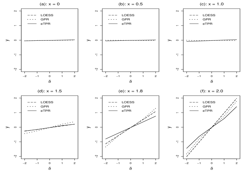
The simulation study result based on 500 replications are reported in Table 1. The performance is measured by the mean squared error between the predictions and the true values for the test data: $MSE=\sum_{j=1}^{J}(\hat{f}_{1}(x_{j}^{\ast})-f_{10}(x_{j}^{\ast}))^{2}/J$. Table 1 shows that the eTPR model performs the best among the three methods: LOESS, GPR and eTPR, and the GPR has comparable MSE with the LOESS, in the presence of outliers. The improvement is greater with large $\sigma^{2}$ as expected. This is also confirmed in Figure 2. Instead of random disturbance, a constant disturbance $\delta$ is added to the training data point 2.0, where $\delta=-2,-1,0,1$ and $2$. Predicted values $\hat{y}_{1}(u)$ at data points $u=0,0.5,1.0,1.5,1.8$ and $2.0$ are calculated respectively by the LOESS, GPR and eTPR. Figure 2 presents the average value of predictions based on 500 replications at each data points against $\delta$. It shows clearly that the influence from outliers is ignorable for the data points in the area less than 1.5, in which there are densely observed data. But the influence becomes larger in the sparse data area $1.5<x\leq 2.0$. Predictions from the eTPR method are shrunken more heavily than those calculated from the other methods in this area.

Table 2: Mean squared errors of prediction results and their standard deviation (in parentheses) by the LOESS, GPR and eTPR methods with $m=1$ and no outliers.
$n$ Model LOESS GPR eTPR
10 (1) 0.044(0.028) 0.034(0.025) 0.035(0.025)
(2) 0.046(0.029) 0.046(0.029) 0.044(0.029)
20 (1) 0.020(0.012) 0.022(0.018) 0.021(0.015)
(2) 0.024(0.014) 0.030(0.018) 0.028(0.017)
30 (1) 0.013(0.009) 0.013(0.011) 0.014(0.009)
(2) 0.016(0.010) 0.021(0.013) 0.020(0.012)
Table 3: Mean squared errors of prediction results and their standard deviation (in parentheses) by the LOESS, GPR and eTPR methods with 6 different simulation setups and $m=1$.
$n$ Model LOESS GPR eTPR
10 (1) 1.241(4.955) 0.158(0.240) 0.089(0.135)
(2) 1.027(3.643) 0.188(0.307) 0.146(0.256)
(3) 0.412(1.584) 0.131(0.198) 0.078(0.077)
(4) 0.415(1.586) 0.147(0.192) 0.110(0.119)
(5) 1.111(4.325) 0.204(0.456) 0.122(0.262)
(6) 1.232(3.553) 0.365(0.400) 0.327(0.443)
20 (1) 0.682(4.497) 0.074(0.125) 0.047(0.064)
(2) 0.515(2.350) 0.089(0.151) 0.074(0.117)
(3) 0.160(0.621) 0.073(0.088) 0.058(0.061)
(4) 0.164(0.621) 0.086(0.089) 0.081(0.094)
(5) 0.290(1.163) 0.086(0.162) 0.068(0.153)
(6) 0.454(1.372) 0.298(0.520) 0.270(0.432)
30 (1) 0.793(6.723) 0.043(0.082) 0.033(0.060)
(2) 0.324(2.643) 0.060(0.119) 0.052(0.107)
(3) 0.186(1.838) 0.053(0.060) 0.045(0.043)
(4) 0.189(1.843) 0.067(0.070) 0.062(0.063)
(5) 0.366(2.764) 0.063(0.144) 0.055(0.127)
(6) 0.533(2.099) 0.256(0.336) 0.246(0.314)

We also investigate robust property against model misspecification and/or outliers in output space. Data $y_{1j}$ are generated from the following 6 process models:
(1) $f_{1}\sim GP(0,k)$, $\epsilon_{1}\sim N(0,\phi)$, $\phi=0.1$, and $\mbox{\boldmath${\theta}$}=(0.05,~{}2,~{}0.05)$;
(2) $f_{1}\sim GP(0,k)$, $\epsilon_{1}\sim N(0,\phi)$, $\phi=0.1$, and $\mbox{\boldmath${\theta}$}=(0.1,~{}4,~{}0.1)$;
(3) $f_{1}\sim GP(0,k)$, $\epsilon_{1}\sim\sqrt{\phi}t_{2}$, $\phi=0.1$, and $\mbox{\boldmath${\theta}$}=(0.05,~{}2,~{}0.05)$;
(4) $f_{1}\sim GP(0,k)$, $\epsilon_{1}\sim\sqrt{\phi}t_{2}$, $\phi=0.1$, and $\mbox{\boldmath${\theta}$}=(0.1,~{}4,~{}0.1)$;
(5) $f_{1}\sim ETP(2,2,0,k)$, $\epsilon_{1}\sim ETP(2,2,0,k_{\epsilon})$, $\phi=0.1$, and $\mbox{\boldmath${\theta}$}=(0.05,~{}2,~{}0.05)$;
(6) $f_{1}$ and $\epsilon_{1}$ has a joint ETP (3) with $\phi=0.1$ and $\mbox{\boldmath${\theta}$}=(0.05,~{}2,~{}0.05)$,
where $k=k_{se}+k_{lin}$. We also take sample size as $n=10$, 20 and 30. In each replication, $N=50$ points are generated evenly spaced in [0, 3.0], denoted by $S$. And $n$ points evenly spaced in $S$ are taken as training data, and the remaining as testing data. Values of mean squared error (MSE) for test data are computed for each of the LOESS, GPR and eTPR methods. Table 2 presents MSEs of LOESS, GPR and eTPR under Cases (1) and (2), where the data are generated from the GPR models and do not exists outliers. It shows that eTPR has comparable performance with GPR. As expected, LOESS is comparable with or slightly better than the other two models for those two simple cases. To study robustness, we consider model misspecifications and outliers in the following ways. For Cases (1), (2) (5) and (6), the $n$th data point from the training data set is added with a $t_{1}$ error. Thus, Cases (1) and (2) have outliers, Cases (3) and (4) have non-normal errors and Cases (5) and (6) have both. We see from Table 3 that the eTPR method performs consistently better than the other two methods, especially when sample size is small. More simulation study results are presented in Table D.11 in Appendix D.

Performance of the eTPR is also investigated by studying data generation model with peak contamination (Sawant et al. (2012)). Under Cases (1), (2), (5) and (6), data $y_{1}(u)$ are contaminated through $\tilde{y}_{1}(u)=y_{1}(u)+4c_{1}\eta_{1}$ if $T_{1}\leq u\leq T_{1}+1/15$, otherwise $\tilde{y}_{1}(u)=y_{1}(u)$, where $c_{1}$ is 1 with probability 0.8 and 0 with probability 0.2, $\eta_{1}$ is independent of $c_{1}$ taking value of 1 or -1 with equal probability of 0.5, $T_{1}$ is random number from a uniform distribution in [0,14/15]; see the details in (Sawant et al. (2012)). Sample size is $n=20$. MSEs of prediction from the LOESS, GPR and eTPR are presented in Table 4. It shows that eTPR has the smallest MSE, and GPR performs better than LOESS.

Table 4: Mean squared errors of prediction results and their standard deviation (in parentheses) by the LOESS, GPR and eTPR methods under peak contamination and $n=20$.
Model LOESS GPR eTPR
(1) 0.142(0.097) 0.085(0.090) 0.065(0.070)
(2) 0.145(0.099) 0.105(0.087) 0.092(0.083)
(5) 0.168(0.115) 0.119(0.112) 0.101(0.120)
(6) 0.353(0.359) 0.303(0.365) 0.286(0.393)
Refer to caption
Figure 3: Predicted values at the data points $x\in\{0.0,~{}0.5,~{}1.0,~{}1.5,~{}1.8,~{}2.0\}$ with $m=2$ and constant disturbance at the point 2.0, where dashed, doted and solid lines respectively represent predictions from the LOESS, GPR and eTPR methods, respectively.

(ii) Models with $m=2$

Now we study the models when $m>1$. We take $m=2$ and kernel functions, $k_{i}=k_{se}+k_{lin},i=1,2$, for both GPR and eTPR models. Based on the previous discussion, GPR and eTPR models under this kernel have different predictions when $m>1$, while they have the same ones when $m=1$.

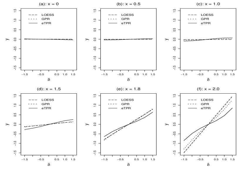
Let us investigate selective shrinkage property of the eTPR firstly. Simulation data are generated similar to the cases of $m=1$, where $f_{i}$, $\epsilon_{i}$, $x_{ij}$ and $y_{ij}$ for each $i$ follow the same setups as those in the constant disturbance case above. Sample sizes are $n_{1}=n_{2}=n=10$. The average predicted values at data points $u=0,0.5,1.0,1.5,1.8$ and $2.0$ are presented in Figure 3. It shows the results similar to the case of $m=1$ in Figure 2. The eTPR model shrinks the prediction at sparse data region much more than the LOESS and GPR models.

Table 5: Mean squared errors of prediction results and their standard deviation (in parentheses) by the LOESS, GPR and eTPR methods with $m=2$ and without outliers. Dimension of the covariates is 1 or 3.
Dimension Model LOESS GPR eTPR($\nu=1.05$) eTPR
1 (1) 0.033(0.034) 0.021(0.015) 0.020(0.015) 0.022(0.016)
(2) 0.065(0.069) 0.043(0.032) 0.042(0.030) 0.041(0.030)
3 (1) 19.111(155.179) 0.061(0.037) 0.059(0.036) 0.061(0.042)
(2) 19.518(154.742) 0.098(0.061) 0.096(0.061) 0.103(0.063)
Table 6: Mean squared errors of prediction results and their standard deviation (in parentheses) by the LOESS, GPR and eTPR methods with $m=2$ and outliers. Dimension of the covariates is 1 or 3.
Dimension Model LOESS GPR eTPR($\nu=1.05$) eTPR
1 (1) 0.257(0.753) 0.160(0.464) 0.152(0.475) 0.139(0.441)
(2) 0.293(0.815) 0.183(0.482) 0.171(0.464) 0.161(0.444)
(3) 0.253(0.799) 0.147(0.511) 0.156(0.760) 0.130(0.495)
(4) 0.398(0.894) 0.247(0.735) 0.227(0.688) 0.222(0.710)
(5) 0.392(1.157) 0.199(0.577) 0.155(0.351) 0.154(0.389)
(6) 0.389(0.555) 0.300(0.435) 0.295(0.440) 0.277(0.440)
3 (1) 26.216(253.396) 0.272(0.919) 0.264(0.909) 0.252(0.922)
(2) 68.825(672.400) 0.246(0.458) 0.242(0.456) 0.230(0.434)
(3) 33.026(412.647) 0.329(0.923) 0.318(0.841) 0.308(0.919)
(4) 25.892(177.680) 0.318(0.503) 0.312(0.446) 0.294(0.430)
(5) 29.432(281.501) 0.298(0.613) 0.293(0.610) 0.285(0.624)
(6) 24.803(219.508) 0.499(0.719) 0.486(0.661) 0.475(0.678)
Table 7: Estimates of $\nu$ with $m=2$ and 1- or 3- dimensional covariates
Dimension (1) (2) (3) (4) (5) (6)
1 3.592(0.912) 3.712(0.803) 3.557(0.938) 3.693(0.819) 3.553 (0.951) 3.471(1.030)
3 3.782(0.692) 3.734(0.742) 3.804(0.650) 3.736(0.768) 3.666(0.854) 3.666(0.832)

We now consider the models with one single explanatory variate in function $f_{i}$, $i=1,2$. Sample sizes are taken as $n_{1}=n_{2}=n=10$. Similar to $m=1$, data $y_{ij}$ are generated from the following 6 process models:
(1) $f_{i}\sim GP(0,k)$, $\epsilon_{i}\sim N(0,\phi)$, $\phi=0.05$, and $\mbox{\boldmath${\theta}$}=(0.025,~{}2,~{}0.025)$;
(2) $f_{i}\sim GP(0,k)$, $\epsilon_{i}\sim N(0,\phi)$, $\phi=0.1$, and $\mbox{\boldmath${\theta}$}=(0.05,~{}2,~{}0.05)$;
(3) $f_{i}\sim GP(0,k)$, $\epsilon_{i}\sim\sqrt{\phi}t_{2}$, $\phi=0.05$, and $\mbox{\boldmath${\theta}$}=(0.025,~{}2,~{}0.025)$;
(4) $f_{i}\sim GP(0,k)$, $\epsilon_{i}\sim\sqrt{\phi}t_{2}$, $\phi=0.1$, and $\mbox{\boldmath${\theta}$}=(0.05,~{}2,~{}0.05)$;
(5) $f_{i}\sim ETP(2,2,0,k)$, $\epsilon_{i}\sim ETP(2,2,0,k_{\epsilon})$, $\phi=0.05$, and $\mbox{\boldmath${\theta}$}=(0.025,~{}2,~{}0.025)$;
(6) $f_{i}$ and $\epsilon_{i}$ has a joint ETP (3) with $\phi=0.05$ and $\mbox{\boldmath${\theta}$}=(0.025,~{}2,~{}0.025)$,
where $k=k_{se}+k_{lin}$, $\mbox{\boldmath${\theta}$}=(\eta_{0},\eta_{1},\xi_{0})$. As before, $N=50$ points evenly spaced in [0, 3.0] are generated, $n=10$ randomly selected points are used as training data and the remaining as testing data. Here the parameter $\nu$ is estimated. As comparison, we also consider the model with fixed value of $\nu=1.05$ (as in the case of $m=1$), denoted by eTPR($\nu=1.05$). Values of mean squared error based on 500 replications are reported for all the four models in the upper panel in Table 5. It shows the results for Cases (1) and (2), where the data are generated from GPR models. We can see that all four methods performs similarly.

To study robustness, in Cases (1), (2), (5) and (6), one data point for each group is randomly selected from the training data set and is added with a $t_{2}$ error. We see from the upper panel in Table 6 that eTPR methods perform better than the LOESS and GPR. And eTPR has smaller MSE than eTPR($\nu=1.05$), indicating a better fit when the parameter $\nu$ can be estimated from the data.

We also study the models with multivariate covariate $\mbox{\boldmath${x}$}=(x_{1},x_{2},x_{3})^{T}$. In this case, $\mbox{\boldmath${\theta}$}=(\eta_{0},\eta_{1},\eta_{2},\eta_{3},\xi_{0},\xi_{1},\xi_{2}),$ where $(\eta_{0},\eta_{1},\eta_{2},\eta_{3})$ are the parameters in the kernel $k_{se}$, and ($\xi_{0},\xi_{1},\xi_{2}$) are the ones in the $k_{lin}$. To generate data, we follow the previous six process models, but $\mbox{\boldmath${\theta}$}=(0.05,~{}2,~{}2,~{}2,~{}0.05,~{}0.05,~{}0.05)$ for Cases 1, 3, 5 and 6, and for Cases 2 and 4, $\mbox{\boldmath${\theta}$}=(0.1,~{}4,~{}4,~{}4,~{}0.1,~{}0.1,~{}0.1)$. Let $S_{1}$, $S_{2}$ and $S_{3}$ be sets of $N=50$ points evenly spaced in the intervals (-2, 2), (0, 3) and (1, 2), respectively. For each group, we randomly take $10$ points as the training data and the remaining as the test data. The lower panel in Table 5 shows the MSEs for Cases (1) and (2), where GPR models are the true models of the generated data. We can see that the eTPR methods have comparable MSEs with the GPR, both perform pretty well. But the LOESS method fails in this case this is because it is designed to deal with the model with a one-dimensional covariate only.

To study robustness, we also randomly select one data point for each group from the training data and add $t_{2}$ errors for Cases (1), (2), (5) and (6). The lower panel in Table 6 presents the values of MSE. Again, the eTPR methods perform better than the GPR method, and the LOESS fails.

Table 7 lists estimates of $\nu$ for 1- and 3- dimensional covaraite. We can see that the estimates of $\nu$ are much larger than $\nu=1.05$, the fixed value we used in the setting and in the case of $m=1$.

More curves are generated to study the performance of prediction from the 4 methods. We take $m=10$ and simulation cases (1) - (6) are the same as those in the situation of $m=2$ and 3-dimensional covariates. For Cases (1), (2), (5) and (6), two curves from $m$ ones are selected, and for each selected curve, one data point is randomly chose from the training data sets and added with a $t_{2}$ error. Table 8 presents the values of MSE and Table 9 lists estimates of $\nu$. These tables shows the similar conclusion with $m=2$. Moreover, MSEs and their standard deviations for GPR and eTPR methods become smaller compared to $m=2$.

Table 8: Mean squared errors of prediction results and their standard deviation (in parentheses) by the LOESS, GPR and eTPR methods with $m=10$ and 3-dimension covariates.
Model LOESS GPR eTPR($\nu=1.05$) eTPR
(1) 27.167(204.574) 0.131(0.547) 0.126(0.543) 0.124(0.541)
(2) 67.839(568.164) 0.164(0.463) 0.161(0.488) 0.154(0.395)
(3) 39.760(373.899) 0.335(0.647) 0.333(0.640) 0.323(0.653)
(4) 64.973(517.224) 0.383(0.893) 0.336(0.563) 0.328(0.579)
(5) 39.024(348.024) 0.146(0.201) 0.142(0.182) 0.136(0.132)
(6) 40.297(350.117) 0.376(0.300) 0.373(0.303) 0.368(0.298)
Table 9: Estimates of $\nu$ with $m=10$ and 3- dimensional covariates
(1) (2) (3) (4) (5) (6)
3.895(0.393) 3.897(0.417) 3.554(0.820) 3.575(0.801) 3.480(0.901) 3.401(0.922)

5.2 Real examples

Refer to caption
Figure 4: Prediction curves from the LOESS, GPR and eTPR methods with kernel $k_{i}=k_{se}+k_{lin}$ for the BLC and CRT data, where circles represent data points, and solid, dotted and dashed lines stand for predictions from the GPR, LOESS and eTPR, respectively.
Refer to caption
Figure 5: Prediction curves from the LOESS, GPR and eTPR methods with kernel $k_{i}=k_{se}+k_{m}$ for the BLC and CRT data, where circles represent data points, and solid, dotted and dashed lines stand for predictions from the GPR, LOESS and eTPR, respectively.
Table 10: Prediction errors and their standard deviation (in parentheses) for the 3 real data sets by the LOESS, GPR and eTPR methods.
kernel Data LOESS GPR eTPR
$k_{se}+k_{lin}$ BLC 0.019(0.006) 0.025(0.017) 0.020(0.006)
CRT 0.049(0.012) 0.062(0.026) 0.049(0.012)
Snow 1.142(0.102) - 1.111(0.105)
Spatial 0.510(0.119) - 0.193(0.075)
$k_{se}+k_{m}$ BLC 0.019(0.006) 0.021(0.009) 0.020(0.006)
CRT 0.049(0.012) 0.054(0.013) 0.049(0.012)
Snow 1.142(0.102) 1.113(0.105) 0.953(0.164)
Spatial 0.510(0.119) 0.203(0.082) 0.197(0.079)

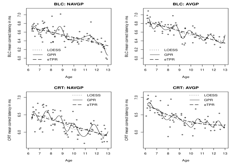
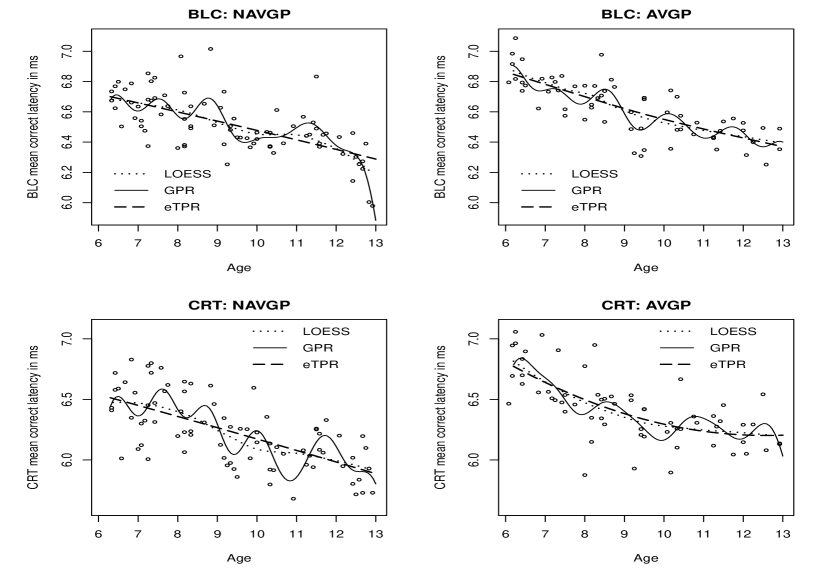
The eTPR model (3) is applied to executive function research data coming from the study in children with Hemiplegic Cerebral Palsy and consisting of 84 girls and 57 boys from primary and secondary schools. These students were subdivided into two groups ($m=2$): the action video game players group (AVGPs) (56%) and the non action video game players group (NAVGPs) (44%). To demonstrate the proposed method, we take 2 measurement indices, Big/Little Circle (BLC) mean correct latency and Choice Reaction Time (CRT) mean correct latency which are investigated as age of children: for more details of this data set, see Xu et al. (2015). Before applying the proposed methods, we take logarithm of BLC and CRT mean correct latencies. For the GPR and eTPR methods, kernel function $k_{i}=k_{se}+k_{lin}$ or $k_{se}+k_{m}$ is used. Figures 4 and 5 present prediction curves under these two kernels, where circles represent observed data points, and solid line, dashed line and dotted line stand for predictions from the GPR, eTPR and LOESS methods, respectively. Estimates of $\nu$ are 6 for eTPR models with either kernel function. We can see prediction curves from the LOESS and eTPR methods are more smooth than those from the GPR method. Furthermore, prediction curves from the GPR method are more influenced by the choice of kernel function compared to those from the eTPR.

We randomly select 80% observation as training data and compute prediction errors for the remaining data points (i.e. the test data). This procedure is repeated 500 times. Table 10 presents mean prediction errors of BLC and CRT mean correct latencies. We can see that the GPR is the worst, while the eTPR is comparable with the LOESS. Again, prediction errors from the GPR more depend on kernel functions compared to the eTPR. Thus, selection of kernel function is more important for the GPR method.

We also apply the three methods to Whistler snowfall data and spatial interpolation data. Those are the models with $m=1$. Whistler snowfall data contain daily snowfall amounts in Whistler for the years 2010 and 2011, and can be downloaded at http://www.climate.weather office.ec.gc.ca. Response for snow data is logarithm of (daily snowfall amount+1) and covariate is time. For spatial interpolation data, rainfall measurements at 467 locations were recorded in Switzerland on 8 May 1986, and can be found at http://www.ai-geostats.org under SIC97. Spatial interpolation data has response, logarithms of (rainfall amount+1), and two covariates for coordinates of location. We also take kernel function $k_{1}=k_{se}+k_{lin}$ or $k_{se}+k_{m}$ for both the GPR and eTPR methods. Prediction errors of the GPR, eTPR and LOESS are listed in Table 10. When $m=1$, results of the eTPR are the same as those of the GPR for kernel $k_{se}+k_{lin}$, so we only list prediction errors of the eTPR in this table. We can see that eTPR has the smallest prediction error. For spatial data with multivariate predictors, the LOESS is much worse. Overall, the eTPR is the best in prediction.

6 Concluding remarks

Advantages of a GPR model include that it offers a nonparametric regression model for data with multi-dimensional covariates, the specification of covariance kernel enables to accommodate a wide class of nonlinear regression functions, and it can be applied to analyze many different types of data including functional data. In this paper, we extended the GPR model to the eTPR model. The latter inherits almost all the good features for the GPR, and additionally it provides robust BLUP procedures in the presence of outliers in both input and output spaces. Even with $m=1$, under some kernels it gives robust prediction. Numerical studies show that the eTPR is overall the best in prediction among the methods considered.

The GPR or eTPR model discussed in this paper is a concurrent functional regression model. The information consistency of the estimation of the unknown $f(\cdot)$ in equation (1) requires dense data, i.e. the sample size tends to infinity. We have shown that eTPR preforms robustly when there are outliers or the data are sparse in some areas. The idea has potential to be extended to a general functional data analysis framework, e.g. scalar-on-function or function-on-function regression model.

Appendix A Properties of extended $t$-process

Let ${\Sigma}$ be an $n\times n$ symmetric and positive definite matrix, $\mbox{\boldmath${\mu}$}\in{R}{{}^{n}}$, $\nu>0$ and $\omega>0$. In this paper, $\mbox{\boldmath${Z}$}\sim EMTD(\nu,\omega,\mbox{\boldmath${\mu}$},\mbox{\boldmath${\Sigma}$})$ means that a random vector $\mbox{\boldmath${Z}$}\in{R}{{}^{n}}$ has the density function,

$$p(z)=|2\pi\omega\mbox{\boldmath${\Sigma}$}|^{-1/2}\frac{\Gamma(n/2+\nu)}{\Gamma(\nu)}\left(1+\frac{\mbox{{\boldmath${(z-\mu)}$}${}^{T}$}\mbox{{\boldmath${\Sigma}$}${}^{{-1}}$}\mbox{\boldmath${(z-\mu)}$}}{2\omega}\right)^{-(n/2+\nu)},$$

where $\Gamma(\cdot)$ is the gamma function.

We may construct an EMTD via a double hierarchical generalized linear model (Lee and Nelder, 2006) as follows:
Lemma 1 If

$$\mbox{\boldmath${Z}$}|r\sim N(\mbox{\boldmath${\mu}$},r\mbox{\boldmath${\Sigma}$}),~{}~{}r\sim\mathrm{IG}(\nu,\omega),$$

where $\mathrm{IG}(\nu,\omega)$ stands for an inverse gamma distribution with the density function

$$g(r)=\frac{1}{\Gamma(\nu)}(\frac{\omega}{r})^{\nu+1}\frac{1}{\omega}\exp{(-\frac{\omega}{r}),}$$

then, marginally $\mbox{\boldmath${Z}$}\sim EMTD(\nu,\omega,\mbox{\boldmath${\mu}$},\mbox{\boldmath${\Sigma}$})$.

Proof: From the construction of ${Z}$, we have

$\displaystyle p(\mbox{\boldmath${z}$})$ $\displaystyle=\int_{0}^{\infty}p(\mbox{\boldmath${z}$}|r)g(r)dr$
$\displaystyle=\int_{0}^{\infty}|2\pi r\mbox{\boldmath${\Sigma}$}|^{-1/2}\exp{(-\frac{(\mbox{\boldmath${z}$}-\mbox{\boldmath${\mu}$})^{T}\mbox{{\boldmath${\Sigma}$}${}^{-1}$}(\mbox{\boldmath${z}$}-\mbox{\boldmath${\mu}$})}{2r})}\frac{1}{\Gamma(\nu)}(\frac{\omega}{r})^{\nu+1}\frac{1}{\omega}\exp{(-\omega/r)}dr$
$\displaystyle=\int_{0}^{\infty}|2\pi\omega\mbox{\boldmath${\Sigma}$}|^{-1/2}\frac{1}{\Gamma(\nu)}(\frac{\omega}{r})^{n/2+\nu-1}\exp{(-\frac{2\omega+(\mbox{\boldmath${z}$}-\mbox{\boldmath${\mu}$})^{T}\mbox{{\boldmath${\Sigma}$}${}^{-1}$}(\mbox{\boldmath${z}$}-\mbox{\boldmath${\mu}$})}{2r})}d\frac{\omega}{r}$
$\displaystyle=|2\pi\omega\mbox{\boldmath${\Sigma}$}|^{-1/2}\frac{\Gamma(n/2+\nu)}{\Gamma(\nu)}\left(1+\frac{(\mbox{\boldmath${z}$}-\mbox{\boldmath${\mu}$})^{T}\mbox{{\boldmath${\Sigma}$}${}^{-1}$}(\mbox{\boldmath${z}$}-\mbox{\boldmath${\mu}$})}{2\omega}\right)^{-(n/2+\nu)},$

which is the density function of EMTD.$\sharp$

Properties of EMTD are as follows.

Lemma 2 Let $\mbox{\boldmath${Z}$}\sim EMTD(\nu,\omega,\mbox{\boldmath${\mu}$},\mbox{\boldmath${\Sigma}$}).$

  • (i)

    If $\omega/\nu\rightarrow\lambda>0$ as $\nu\rightarrow\infty$, then $\lim_{\nu\rightarrow\infty}EMTD(\nu,\omega,\mbox{\boldmath${\mu}$},\mbox{\boldmath${\Sigma}$})=N(\mu,\lambda\mbox{\boldmath${\Sigma}$}).$

  • (ii)

    For any matrix $\mbox{\boldmath${A}$}\in R^{l\times n}$ with rank $l\leq n$, $\mathit{{\mbox{\boldmath${A}$}\mbox{\boldmath${Z}$}\sim EMTD(\nu,\omega,\mbox{\boldmath${A}$}\mu,\mbox{\boldmath${A}$}\mbox{\boldmath${\Sigma}$}\mbox{{\boldmath${A}$}${}^{T}$})}.\ }$

  • (iii)

    Let ${Z}$ be partitioned as ${(\mbox{{\boldmath${Z}$}${}_{1}^{T}$},\mbox{{\boldmath${Z}$}${}_{2}^{T}$})}^{T}$ with lengths $n_{1}$ and $n_{2}=n-n_{1}$, and ${\mu}$ and ${\Sigma}$ have the corresponding partitions as $\mbox{\boldmath${\mu}$}=(\mbox{{\boldmath${\mu}$}${}_{1}^{T}$},\mbox{{\boldmath${\mu}$}${}_{2}^{T}$})^{T}$ and $\mbox{\boldmath${\Sigma}$}=\left(\begin{array}[]{cc}\mbox{{\boldmath${\Sigma}$}${}_{{11}}$}&\mbox{{\boldmath${\Sigma}$}${}_{{12}}$}\\ \mbox{{\boldmath${\Sigma}$}${}_{{12}}^{T}$}&\mbox{{\boldmath${\Sigma}$}${}_{{22}}$}\end{array}\right)$. Then,

    $\displaystyle\mathit{\mbox{{\boldmath${Z}$}${}_{1}$}\sim EMTD(\nu,\omega,\mbox{{\boldmath${\mu}$}${}_{1}$},\mbox{{\boldmath${\Sigma}$}${}_{{11}}$}),}$
    $\displaystyle\mathit{\mbox{{\boldmath${Z}$}${}_{2}$}|\mbox{{\boldmath${Z}$}${}_{1}$}=\mbox{{\boldmath${z}$}${}_{1}$}\sim EMTD(\nu^{\ast},\omega^{\ast},\mbox{\boldmath${\mu}$}^{\ast},\mbox{\boldmath${\Sigma}$}^{\ast})},$

    with $\nu^{\ast}=n_{1}/2+\nu$, $\omega^{\ast}=n_{1}/2+\omega$, $\mbox{{\boldmath${\mu}$}${}^{*}$}=\mbox{{\boldmath${\Sigma}$}${}_{{12}}^{T}$}\mbox{{\boldmath${\Sigma}$}${}_{{11}}^{{-1}}$}(\mbox{{\boldmath${z}$}${}_{1}$}-\mbox{{\boldmath${\mu}$}${}_{1}$})+\mbox{{\boldmath${\mu}$}${}_{2}$},$ $\mbox{{\boldmath${\Sigma}$}${}^{*}$}=(2\omega+(\mbox{{\boldmath${z}$}${}_{1}$}-\mbox{{\boldmath${\mu}$}${}_{1}$})^{T}\mbox{{\boldmath${\Sigma}$}${}_{{11}}^{{-1}}$}(\mbox{{\boldmath${z}$}${}_{1}$}-\mbox{{\boldmath${\mu}$}${}_{1}$}))\mbox{{\boldmath${\Sigma}$}${}_{{22\cdot 1}}$}/({2\omega+n_{1}}),$ and $\mbox{{\boldmath${\Sigma}$}${}_{{22\cdot 1}}$}=\mbox{{\boldmath${\Sigma}$}${}_{{22}}$}-\mbox{{\boldmath${\Sigma}$}${}_{{12}}^{T}$}\mbox{{\boldmath${\Sigma}$}${}_{{11}}^{{-1}}$}\mbox{{\boldmath${\Sigma}$}${}_{{12}}$}$. This gives $E(\mbox{{\boldmath${Z}$}${}_{2}$}|\mbox{{\boldmath${Z}$}${}_{1}$})=\mbox{{\boldmath${\mu}$}${}^{*}$}\text{{\ and }}Cov(\mbox{{\boldmath${Z}$}${}_{2}$}|\mbox{{\boldmath${Z}$}${}_{1}$})={\omega^{\ast}}\mbox{{\boldmath${\Sigma}$}${}^{*}$}/({\nu^{\ast}-1}).$

  • (iv)

    Let $r$ be a random effect in Lemma 1. Then, $r|\mbox{\boldmath${Z}$}\sim\mathrm{IG}(\tilde{\nu},\tilde{\omega})$ with $\tilde{\nu}=n/2+\nu,$ $\tilde{\omega}=\omega+(\mbox{\boldmath${Z}$}-\mbox{\boldmath${\mu}$})^{T}\mbox{{\boldmath${\Sigma}$}${}^{{-1}}$}(\mbox{\boldmath${Z}$}-\mbox{\boldmath${\mu}$})/2$ and

    $\displaystyle E(r|\mbox{\boldmath${Z}$})=\frac{2\omega+(\mbox{\boldmath${Z}$}-\mbox{\boldmath${\mu}$})^{T}\mbox{{\boldmath${\Sigma}$}${}^{{-1}}$}(\mbox{\boldmath${Z}$}-\mbox{\boldmath${\mu}$})}{n+2\nu-2},$
    $\displaystyle Var(r|\mbox{\boldmath${Z}$})=\frac{(2\omega+(\mbox{\boldmath${Z}$}-\mbox{\boldmath${\mu}$})^{T}\mbox{{\boldmath${\Sigma}$}${}^{{-1}}$}(\mbox{\boldmath${Z}$}-\mbox{\boldmath${\mu}$}))^{2}}{(n+2\nu-2)^{2}(n/2+\nu-2)}.$

Proof: The conclusions (i), (ii) and $\mbox{{\boldmath${Z}$}${}_{1}$}\sim EMTD(\nu,\omega,\mbox{\boldmath${\mu}$}_{1},\mbox{{\boldmath${\Sigma}$}${}_{11}$})$ in (iii) are easily obtained by the definition of EMTD and Lemma 1. Now we only prove that $\mbox{{\boldmath${Z}$}${}_{2}$}|\mbox{{\boldmath${Z}$}${}_{1}$}\sim EMTD(\nu^{\ast},\omega^{\ast},\mbox{{\boldmath${\mu}$}${}^{*}$},\mbox{{\boldmath${\Sigma}$}${}^{*}$})$. Let $a_{1}=(\mbox{{\boldmath${z}$}${}_{1}$}-\mbox{{\boldmath${\mu}$}${}_{1}$})^{T}\mbox{{\boldmath${\Sigma}$}${}_{11}^{-1}$}(\mbox{{\boldmath${z}$}${}_{1}$}-\mbox{{\boldmath${\mu}$}${}_{1}$})$ and $a_{2}=(\mbox{{\boldmath${z}$}${}_{2}$}-\mbox{{\boldmath${\mu}$}${}^{*}$})^{T}\mbox{{\boldmath${\Sigma}$}${}^{*-1}$}(\mbox{{\boldmath${z}$}${}_{2}$}-\mbox{{\boldmath${\mu}$}${}^{*}$})$, then $a_{1}+a_{2}=(\mbox{\boldmath${z}$}-\mbox{\boldmath${\mu}$})^{T}\mbox{{\boldmath${\Sigma}$}${}^{-1}$}(\mbox{\boldmath${z}$}-\mbox{\boldmath${\mu}$})$. We have

$\displaystyle p(\mbox{{\boldmath${z}$}${}_{2}$}|\mbox{{\boldmath${z}$}${}_{1}$})=\frac{p(\mbox{\boldmath${z}$})}{p(\mbox{{\boldmath${z}$}${}_{1}$})}$
$\displaystyle=$ $\displaystyle\frac{|2\pi\omega\mbox{\boldmath${\Sigma}$}|^{-1/2}\frac{\Gamma(n/2+\nu)}{\Gamma(\nu)}\left(1+\frac{a_{1}+a_{2}}{2\omega}\right)^{-(n/2+\nu)}}{|2\pi\omega\mbox{{\boldmath${\Sigma}$}${}_{11}$}|^{-1/2}\frac{\Gamma(n_{1}/2+\nu)}{\Gamma(\nu)}\left(1+\frac{a_{1}}{2\omega}\right)^{-(n_{1}/2+\nu)}}\propto\left(1+\frac{a_{2}}{2\omega+a_{1}}\right)^{-(n/2+\nu)},$

which indicates $\mbox{{\boldmath${Z}$}${}_{2}$}|\mbox{{\boldmath${Z}$}${}_{1}$}\sim EMTD(\nu^{\ast},\omega^{\ast},\mbox{{\boldmath${\mu}$}${}^{*}$},\mbox{{\boldmath${\Sigma}$}${}^{*}$})$.

By combining definitions of IG and EMTD, we have

$\displaystyle p(r|\mbox{\boldmath${Z}$})=\frac{p(\mbox{\boldmath${Z}$}|r)g(r)}{p(\mbox{\boldmath${Z}$})}$
$\displaystyle=\frac{1}{\Gamma(n/2+\nu)}\frac{1}{\omega+(\mbox{\boldmath${Z}$}-\mbox{\boldmath${\mu}$})^{T}\mbox{{\boldmath${\Sigma}$}${}^{-1}$}(\mbox{\boldmath${Z}$}-\mbox{\boldmath${\mu}$})/2}\left(\frac{\omega+(\mbox{\boldmath${Z}$}-\mbox{\boldmath${\mu}$})^{T}\mbox{{\boldmath${\Sigma}$}${}^{-1}$}(\mbox{\boldmath${Z}$}-\mbox{\boldmath${\mu}$})/2}{r}\right)^{n/2+\nu+1}$
$\displaystyle\exp{\left(-\frac{\omega+(\mbox{\boldmath${Z}$}-\mbox{\boldmath${\mu}$})^{T}\mbox{{\boldmath${\Sigma}$}${}^{-1}$}(\mbox{\boldmath${Z}$}-\mbox{\boldmath${\mu}$})/2}{r}\right)},$

which indicates (iv) holds in this Lemma.$\sharp$

Proof of Proposition 1: Proposition 1 can be easily proved by using Lemma 2, so omitted here.$\sharp$

Appendix B Properties of eTPR model

B.1 Parameter estimation

Let $\mbox{\boldmath${\beta}$}=(\phi,\mbox{\boldmath${\theta}$}_{1},...,\mbox{\boldmath${\theta}$}_{m})$, where $\phi$ is a parameter for $\epsilon(\mbox{\boldmath${x}$})$ and $\mbox{\boldmath${\theta}$}_{i}$ are those for $f_{i}(\mbox{{\boldmath${x}$}})$ (parameter in the kernel $k_{i}$), $i=1,...,m$. We know that $\mbox{{\boldmath${y}$}${}_{i}$}|\mbox{{\boldmath${X}$}${}_{i}$}\sim EMTD(\nu,\nu-1,0,\mbox{{\boldmath${{\Sigma}}$}${}_{in}$})$ with $\mbox{{\boldmath${\Sigma}$}${}_{in}$}=\mbox{{\boldmath${K}$}${}_{in}$}+\phi\mbox{{\boldmath${I}$}${}_{n}$}$, $\mbox{{\boldmath${K}$}${}_{in}$}=(k_{ijl})_{n\times n}$ and $k_{ijl}=k_{i}(\mbox{{\boldmath${x}$}${}_{ij}$},\mbox{{\boldmath${x}$}${}_{il}$})$. For given $\nu$, the marginal log-likelihood of ${\beta}$ is

$\displaystyle l(\mbox{\boldmath${\beta}$};\nu)=$ $\displaystyle\sum_{i=1}^{m}\Big{\{}-\frac{n}{2}\log(2\pi(\nu-1))-\frac{1}{2}\log|\mbox{{\boldmath${{\Sigma}}$}${}_{in}$}|{-(\frac{n}{2}+\nu)}\log\left(1+\frac{S_{i}}{2(\nu-1)}\right)$
$\displaystyle+\log(\Gamma(\frac{n}{2}+\nu))-\log(\Gamma(\nu))\Big{\}},$

where $S_{i}=\mbox{{\boldmath${y}$}${}_{i}^{T}$}\mbox{{\boldmath${{\Sigma}}$}${}_{in}^{-1}$}\mbox{{\boldmath${y}$}${}_{i}$}$. The score function of $\beta_{k}$, the $k$th element of ${\beta}$, is

$$\frac{\partial l(\mbox{\boldmath${\beta}$};\nu)}{\partial\beta_{k}}=\frac{1}{2}\sum_{i=1}^{m}Tr\left(\Big{(}s_{1i}\mbox{\boldmath${\alpha}_{i}$}\mbox{{\boldmath${\alpha}_{i}$}${}^{T}$}-\mbox{{\boldmath${{\Sigma}}$}${}_{in}^{-1}$}\Big{)}\frac{\partial\mbox{{\boldmath${{\Sigma}}$}${}_{in}$}}{\partial\beta_{k}}\right),$$ (9)

where $\mbox{{\boldmath${\alpha}$}${}_{i}$}=\mbox{{\boldmath${{\Sigma}}$}${}_{in}^{-1}$}\mbox{{\boldmath${y}$}${}_{i}$}$, and $s_{1i}=({n+2\nu})/({2(\nu-1)+S_{i}})$.

A maximum likelihood (ML) estimate of ${\beta}$ can be learned by using gradient based methods, denoted by $\hat{\mbox{\boldmath${\beta}$}}$. The first derivative is given in (9) and the second derivative of $l(\mbox{\boldmath${\beta}$};\nu)$ with respect to ${\beta}$ is,

$\displaystyle\frac{\partial^{2}l(\mbox{\boldmath${\beta}$};\nu)}{\partial\beta_{k}\partial\beta_{k}}=\frac{1}{2}\sum_{i=1}^{m}Tr\left(\Big{(}s_{1i}\mbox{{\boldmath${\alpha}$}${}_{i}$}\mbox{{\boldmath${\alpha}$}${}_{i}^{T}$}-\mbox{{\boldmath${{\Sigma}}$}${}_{in}^{-1}$}\Big{)}\Big{(}\frac{\partial^{2}\mbox{{\boldmath${{\Sigma}}$}${}_{in}$}}{\partial\beta_{k}\partial\beta_{k}}-\frac{\partial\mbox{{\boldmath${{\Sigma}}$}${}_{in}$}}{\partial\beta_{k}}\mbox{{\boldmath${{\Sigma}}$}${}_{in}^{-1}$}\frac{\partial\mbox{{\boldmath${{\Sigma}}$}${}_{in}$}}{\partial\beta_{k}}\Big{)}\right)$
$\displaystyle-\frac{1}{2}Tr\left(s_{1i}\mbox{{\boldmath${\alpha}$}${}_{i}$}\mbox{{\boldmath${\alpha}$}${}_{i}^{T}$}\frac{\partial\mbox{{\boldmath${{\Sigma}}$}${}_{in}$}}{\partial\beta_{k}}\mbox{{\boldmath${{\Sigma}}$}${}_{in}^{-1}$}\frac{\partial\mbox{{\boldmath${{\Sigma}}$}${}_{in}$}}{\partial\beta_{k}}\right)+\frac{1}{2}\frac{s_{1i}^{2}}{n+2\nu}\left\{Tr\left(\mbox{{\boldmath${\alpha}$}${}_{i}$}\mbox{{\boldmath${\alpha}$}${}_{i}^{T}$}\frac{\partial\mbox{{\boldmath${{\Sigma}}$}${}_{in}$}}{\partial\beta_{k}}\right)\right\}^{2}.$ (10)

Thus, variance of $\hat{\beta}_{k}$ can be estimated by using $\Big{(}-\frac{\partial^{2}l(\mbox{\boldmath${\beta}$};\nu)}{\partial\beta_{k}\partial\beta_{k}}\Big{)}^{-1}\Big{|}_{\mbox{\boldmath${\beta}$}=\hat{\mbox{\boldmath${\beta}$}}}$, where $\hat{\beta}_{k}$ is the $k$th component of $\hat{\mbox{\boldmath${\beta}$}}$.

B.2 Prediction

The five covariance kernels are given as follows, (Rasmussen and Williams, 2006; Shi and Choi, 2011), for $\mbox{\boldmath${u}$},\mbox{\boldmath${v}$}\in R^{p}$,

  • 1.

    Squared exponential kernel:

    $\displaystyle k_{se}(\mbox{\boldmath${u}$},\mbox{\boldmath${v}$})=\eta_{0}\exp{\left(-\frac{1}{2}\sum_{l=1}^{p}\eta_{l}(u_{l}-v_{l})^{2}\right)},$

    where $\eta_{l}>0$, $l=0,1,...,p$.

  • 2.

    Non-stationary linear kernel:

    $\displaystyle k_{lin}(\mbox{\boldmath${u}$},\mbox{\boldmath${v}$})=\sum_{l=1}^{p}\eta_{l-1}u_{l}v_{l},$

    where $\eta_{l}>0$, $l=0,...,p-1$.

  • 3.

    von Mises-inspired kernel:

    $\displaystyle k_{vm}(\mbox{\boldmath${u}$},\mbox{\boldmath${v}$})=\eta_{0}\exp{\left(\eta_{1}\Big{(}\sum_{l=1}^{p}\cos(u_{l}-v_{l})-p\Big{)}\right)},$

    where $\eta_{0}>0$ and $\eta_{1}>0$.

  • 4.

    Rational quadratic kernel:

    $\displaystyle k_{rq}(\mbox{\boldmath${u}$},\mbox{\boldmath${v}$})=\left(1+(20^{1/\lambda}-1)\sum_{l=1}^{p}\eta_{l}(u_{l}-v_{l})^{2}\right)^{-\lambda},$

    where $\lambda>0$ and $\eta_{l}>0$, $l=1,...,p$.

  • 5.

    Mat$\acute{e}$rn kernel: for a known $\alpha$,

    $\displaystyle k_{m}(\mbox{\boldmath${u}$},\mbox{\boldmath${v}$})=\frac{1}{\Gamma(\alpha)2^{\alpha-1}}(\eta_{1}\|\mbox{\boldmath${u}$}-\mbox{\boldmath${v}$}\|)^{\alpha}\mathcal{K}_{\alpha}(\eta_{1}\|\mbox{\boldmath${u}$}-\mbox{\boldmath${v}$}\|),$

    where $\eta_{1}>0$ and $\mathcal{K}_{\alpha}(\cdot)$ is a modified Bessel function of order $\alpha$. When $\alpha=3/2$,

    $$k_{m}(\mbox{\boldmath${u}$},\mbox{\boldmath${v}$})=(1+\eta_{1}(\sum_{l=1}^{p}(u_{l}-v_{l})^{2})^{1/2})\exp{(-\eta_{1}(\sum_{l=1}^{p}(u_{l}-v_{l})^{2})^{1/2})}.$$

Proof of Proposition 2: We show that under the kernel functions $k_{se}$, $k_{lin}$ and $k_{vm}$, when $\eta_{0}$ is unknown and estimated, the predictions of $f_{1}(\mbox{{\boldmath${X}$}${}_{1}$})$ and $f_{1}(\mbox{\boldmath${u}$})$ from eTPR models have the same values as those from GPR models. When $\eta_{0}$ is a constant such as $\eta_{0}=1$, eTPR models under each of above kernels have different predictions to those from GPR models. We take the squared exponential kernel and the rational quadratic kernel as examples to prove the properties.

Under the squared exponential kernel $k_{1}=k_{se}$, we can reparametrize the kernel function $k_{1}$ as ${k}_{1}^{*}=k_{1}/\phi$, that is

$\displaystyle{k}_{1}^{*}(\mbox{\boldmath${u}$},\mbox{\boldmath${v}$})={\eta}^{*}_{0}\exp{\left(-\frac{1}{2}\sum_{l=1}^{p}\eta_{l}(u_{l}-v_{l})^{2}\right)},$

where ${\eta}^{*}_{0}=\eta_{0}/\phi$. Thus, we can rewrite

$$\left(\begin{array}[]{c}f_{1}\\ \epsilon_{1}\end{array}\right)\sim ETP\left(\nu,\nu-1,\left(\begin{array}[]{c}0\\ 0\end{array}\right),\phi\left(\begin{array}[]{cc}{k}_{1}^{*}&0\\ 0&I_{1}\end{array}\right)\right),$$

where $I_{1}(\mbox{\boldmath${u}$},\mbox{\boldmath${v}$})=I(\mbox{\boldmath${u}$}=\mbox{\boldmath${v}$})$.

Let $\mbox{\boldmath${\theta}$}^{*}_{1}=\{\eta^{*}_{0},\eta_{l},l=1,...,p\}$, and $\mbox{\boldmath${\beta}$}^{*}=(\phi,\mbox{{\boldmath${\theta}$}${}_{1}^{*T}$})^{T}$. Under this reparametrization, for a new data point $\mbox{\boldmath${x}$}=\mbox{\boldmath${u}$}$, the prediction of $f_{1}(\mbox{{\boldmath${u}$}})$ becomes

$\displaystyle E(f_{1}(\mbox{{\boldmath${u}$}})|\mbox{{\boldmath${\cal D}$}${}_{n}$})={\mbox{\boldmath${k}$}}_{1u}\mbox{{\boldmath${\Sigma}$}${}_{1n}^{-1}$}\mbox{{\boldmath${y}$}}_{1}={\mbox{\boldmath${k}$}}^{*}_{1u}\mbox{{\boldmath${H}$}${}_{1n}^{-1}$}\mbox{{\boldmath${y}$}}_{1},$

where ${\mbox{\boldmath${k}$}}_{1u}=(k_{1}(\mbox{{\boldmath${x}$}${}_{11}$},\mbox{\boldmath${u}$}),...,k_{1}(\mbox{{\boldmath${x}$}${}_{1n}$},\mbox{\boldmath${u}$}))^{T}$, ${\mbox{\boldmath${k}$}}^{*}_{1u}=({k}_{1}^{*}(\mbox{{\boldmath${x}$}${}_{11}$},\mbox{\boldmath${u}$}),...,{k}_{1}^{*}(\mbox{{\boldmath${x}$}${}_{1n}$},\mbox{\boldmath${u}$}))^{T}$, ${\mbox{\boldmath${K}$}}^{*}_{1n}=({k}_{1}^{*}(\mbox{{\boldmath${x}$}${}_{1i}$},\mbox{{\boldmath${x}$}${}_{1j}$}))_{n\times n}$ and $\mbox{{\boldmath${H}$}${}_{1n}$}={\mbox{\boldmath${K}$}}^{*}_{1n}+\mbox{{\boldmath${I}$}${}_{n}$}$. We can see this prediction only depends on ${\eta}^{*}_{0}$ and ${\eta}_{l}$. The predictive covariance under the eTPR model is

$\displaystyle Var(f_{1}(\mbox{{\boldmath${u}$}})|\mbox{{\boldmath${\cal D}$}${}_{n}$})=s_{01}(k_{1}(\mbox{\boldmath${u}$},\mbox{\boldmath${u}$})-{\mbox{\boldmath${k}$}}_{1u}^{T}\mbox{{\boldmath${\Sigma}$}${}_{1n}^{-1}$}{\mbox{\boldmath${k}$}}_{1u})=s_{01}\phi({k}_{1}^{*}(\mbox{\boldmath${u}$},\mbox{\boldmath${u}$})-{{\mbox{\boldmath${k}$}}}_{1u}^{*T}\mbox{{\boldmath${H}$}${}_{1n}^{-1}$}{{\mbox{\boldmath${k}$}}}^{*}_{1u}),$
$\displaystyle s_{01}=\frac{\mbox{{\boldmath${y}$}${}_{1}^{T}$}\mbox{{\boldmath${\Sigma}$}${}_{1n}^{-1}$}\mbox{{\boldmath${y}$}}_{1}+2(\nu-1)}{n+2(\nu-1)}=\frac{\phi^{-1}\mbox{{\boldmath${y}$}${}_{1}^{T}$}\mbox{{\boldmath${H}$}${}_{1n}^{-1}$}\mbox{{\boldmath${y}$}}_{1}+2(\nu-1)}{n+2(\nu-1)},$

which indicates that it depends on ${\eta}^{*}_{0}$, ${\eta}_{l}$, $\phi$ and $\nu$.

From (9), letting the score function of $\phi$ be 0, we obtain

$\displaystyle s_{11}\phi^{-1}=\frac{n}{\mbox{{\boldmath${y}$}${}_{1}^{T}$}\mbox{{\boldmath${H}$}${}_{1n}^{-1}$}\mbox{{\boldmath${y}$}}_{1}}.$

It gives a ML estimator of $\phi$ as

$\displaystyle\hat{\phi}=\frac{\nu}{\nu-1}\frac{\mbox{{\boldmath${y}$}${}_{1}^{T}$}\mbox{{\boldmath${H}$}${}_{1n}^{-1}$}\mbox{{\boldmath${y}$}${}_{1}$}}{n}=\frac{\nu}{\nu-1}\tilde{\phi},$

where $\tilde{\phi}$ is ML estimator of $\phi$ under the GPR model ($s_{11}=1$).

For $\eta_{l}$ and ${\eta}^{*}_{0}$, we have their score equations,

$\displaystyle\frac{\partial l(\mbox{\boldmath${\beta}$}^{*};\nu)}{\partial\eta_{l}}=\frac{\partial l(\mbox{\boldmath${\beta}$};\nu)}{\partial\eta_{l}}=$ $\displaystyle\frac{1}{2}Tr\left(\Big{(}s_{11}\phi^{-1}\mbox{{\boldmath${H}$}${}_{1n}^{-1}$}\mbox{{\boldmath${y}$}${}_{1}$}\mbox{{\boldmath${y}$}${}_{1}^{T}$}\mbox{{\boldmath${H}$}${}_{1n}^{-1}$}-\mbox{{\boldmath${H}$}${}_{1n}^{-1}$}\Big{)}\frac{\partial\mbox{{\boldmath${H}$}${}_{1n}$}}{\partial\eta_{l}}\right)=0,$
$\displaystyle\frac{\partial l(\mbox{\boldmath${\beta}$}^{*};\nu)}{\partial{\eta}^{*}_{0}}=\frac{\partial l(\mbox{\boldmath${\beta}$};\nu)}{\partial{\eta}^{*}_{0}}=$ $\displaystyle\frac{1}{2}Tr\left(\Big{(}s_{11}\phi^{-1}\mbox{{\boldmath${H}$}${}_{1n}^{-1}$}\mbox{{\boldmath${y}$}${}_{1}$}\mbox{{\boldmath${y}$}${}_{1}^{T}$}\mbox{{\boldmath${H}$}${}_{1n}^{-1}$}-\mbox{{\boldmath${H}$}${}_{1n}^{-1}$}\Big{)}\frac{\partial\mbox{{\boldmath${H}$}${}_{1n}$}}{\partial{\eta}^{*}_{0}}\right)=0.$

Thus, we have

$\displaystyle\frac{\partial l(\mbox{\boldmath${\beta}$}^{*};\nu)}{\partial\eta_{l}}=\frac{1}{2}Tr\left(\Big{(}\frac{n}{\mbox{{\boldmath${y}$}${}_{1}^{T}$}\mbox{{\boldmath${H}$}${}_{1n}^{-1}$}\mbox{{\boldmath${y}$}}_{1}}\mbox{{\boldmath${H}$}${}_{1n}^{-1}$}\mbox{{\boldmath${y}$}${}_{1}$}\mbox{{\boldmath${y}$}${}_{1}^{T}$}\mbox{{\boldmath${H}$}${}_{1n}^{-1}$}-\mbox{{\boldmath${H}$}${}_{1n}^{-1}$}\Big{)}\frac{\partial\mbox{{\boldmath${H}$}${}_{1n}$}}{\partial\eta_{l}}\right)=0,$ (11)
$\displaystyle\frac{\partial l(\mbox{\boldmath${\beta}$}^{*};\nu)}{\partial{\eta}^{*}_{0}}=\frac{1}{2}Tr\left(\Big{(}\frac{n}{\mbox{{\boldmath${y}$}${}_{1}^{T}$}\mbox{{\boldmath${H}$}${}_{1n}^{-1}$}\mbox{{\boldmath${y}$}}_{1}}\mbox{{\boldmath${H}$}${}_{1n}^{-1}$}\mbox{{\boldmath${y}$}${}_{1}$}\mbox{{\boldmath${y}$}${}_{1}^{T}$}\mbox{{\boldmath${H}$}${}_{1n}^{-1}$}-\mbox{{\boldmath${H}$}${}_{1n}^{-1}$}\Big{)}\frac{\partial\mbox{{\boldmath${H}$}${}_{1n}$}}{\partial{\eta}^{*}_{0}}\right)=0.$ (12)

We can see that the score equations (11) and (12) for $\eta_{l}$ and ${\eta}^{*}_{0}$ do not depend on $\nu$ and $s_{11}$, and they are the same as those under the GPR model. Therefore, the parameters ${\eta}^{*}_{0}$, $\eta_{l}$ under the eTPR model are estimated with the same values as those under the GPR model, which leads to the same prediction of $f_{1}(\mbox{\boldmath${u}$})$.

Plugging $\hat{\phi}$ in $Var(f_{1}(\mbox{{\boldmath${u}$}})|\mbox{{\boldmath${\cal D}$}${}_{n}$})$, we have

$\displaystyle Var(f_{1}(\mbox{{\boldmath${u}$}})|\mbox{{\boldmath${\cal D}$}${}_{n}$})=$ $\displaystyle\frac{n+2\nu}{n+2(\nu-1)}\tilde{\phi}({k}_{1}^{*}(\mbox{\boldmath${u}$},\mbox{\boldmath${u}$})-{{\mbox{\boldmath${k}$}}}_{1u}^{*T}\mbox{{\boldmath${H}$}${}_{1n}^{-1}$}{{\mbox{\boldmath${k}$}}}_{1u}^{*})$
$\displaystyle=$ $\displaystyle\frac{n+2\nu}{n+2(\nu-1)}\widetilde{Var}(f_{1}(\mbox{{\boldmath${u}$}})|\mbox{{\boldmath${\cal D}$}${}_{n}$}),$

where $\widetilde{Var}(f_{1}(\mbox{{\boldmath${u}$}})|\mbox{{\boldmath${\cal D}$}${}_{n}$})$ is conditional variance of $f_{1}(\mbox{{\boldmath${u}$}})$ under GPR model. It follows that the eTPR has slightly bigger variance estimate of the predictor than the GPR.

Under the rational quadratic kernel $k_{1}=k_{rq}$, the score equations for $\phi$, $\lambda$ and $\eta_{l}$ are

$\displaystyle\frac{\partial l(\mbox{\boldmath${\beta}$};\nu)}{\partial\phi}=\frac{1}{2}Tr\left(s_{11}\mbox{{\boldmath${\alpha}$}${}_{1}$}\mbox{{\boldmath${\alpha}$}${}_{1}^{T}$}-\mbox{{\boldmath${{\Sigma}}$}${}_{1n}^{-1}$}\right)=0,$
$\displaystyle\frac{\partial l(\mbox{\boldmath${\beta}$};\nu)}{\partial\lambda}=\frac{1}{2}Tr\left(\Big{(}s_{11}\mbox{{\boldmath${\alpha}$}${}_{1}$}\mbox{{\boldmath${\alpha}$}${}_{1}^{T}$}-\mbox{{\boldmath${{\Sigma}}$}${}_{1n}^{-1}$}\Big{)}\frac{\partial\mbox{{\boldmath${{\Sigma}}$}${}_{1n}$}}{\partial\lambda}\right)=0,$
$\displaystyle\frac{\partial l(\mbox{\boldmath${\beta}$};\nu)}{\partial\eta_{l}}=\frac{1}{2}Tr\left(\Big{(}s_{11}\mbox{{\boldmath${\alpha}$}${}_{1}$}\mbox{{\boldmath${\alpha}$}${}_{1}^{T}$}-\mbox{{\boldmath${{\Sigma}}$}${}_{1n}^{-1}$}\Big{)}\frac{\partial\mbox{{\boldmath${{\Sigma}}$}${}_{1n}$}}{\partial\eta_{l}}\right)=0,$

which are different from those under the GPR model. Hence, the eTPR model has the different estimate value of ${\beta}$ from the GPR model.

Note that

$$s_{01}=\frac{\mbox{{\boldmath${y}$}${}_{1}^{T}$}\mbox{{\boldmath${\Sigma}$}${}_{1n}^{-1}$}\mbox{{\boldmath${y}$}${}_{1}$}+2(\nu-1)}{n+2(\nu-1)}=\frac{(\mbox{{\boldmath${y}$}${}_{1}$}-\hat{\mbox{\boldmath${f}$}}_{1n})^{T}\mbox{{\boldmath${\Sigma}$}${}_{1n}$}(\mbox{{\boldmath${y}$}${}_{1}$}-\hat{\mbox{\boldmath${f}$}}_{1n})/\phi^{2}+2(\nu-1)}{n+2(\nu-1)},$$

where $\hat{\mbox{\boldmath${f}$}}_{1n}=\mbox{{\boldmath${\mu}$}${}_{1n}$}$ is the prediction for $f_{1}(\mbox{{\boldmath${X}$}${}_{1}$})$. Thus, the predictive variance under the eTPR model decreases if the model fits the responses ${y}$i better while that under the GPR model is still independent of the model fit.$\sharp$

Proof of Proposition 3:

When $m>1$ such as $m=2$, we use combination of $k_{i}=k_{se}+k_{lin}$ as an example to illustrate our methods, that is

$\displaystyle k_{i}(\mbox{\boldmath${u}$},\mbox{\boldmath${v}$})=k(\mbox{\boldmath${u}$},\mbox{\boldmath${v}$};\mbox{\boldmath${\theta}_{i}$})=\eta_{i0}\exp{\left(-\frac{1}{2}\sum_{l=1}^{p}\eta_{il}(u_{l}-v_{l})^{2}\right)}+\sum_{l=1}^{p}\xi_{il}u_{l}v_{l},$ (13)

where $\mbox{\boldmath${\theta}$}_{i}=\{\eta_{i0},\eta_{il},\xi_{il},l=1,...,p\}$ are a set of parameters. Let parameter $\mbox{\boldmath${\beta}$}=(\phi,\mbox{{\boldmath${\theta}$}${}_{1}^{T}$},\mbox{{\boldmath${\theta}$}${}_{2}^{T}$})^{T}$. The predictions from both GPR and eTPR are exactly the same under this kernel when $m=1$.

From (9), similar to the case with $m=1$, the score equation of $\phi$ becomes

$\displaystyle\phi=\frac{1}{2n}\sum_{i=1}^{2}s_{1i}\mbox{{\boldmath${y}$}${}_{i}^{T}$}\mbox{{\boldmath${H}$}${}_{in}^{-1}$}\mbox{{\boldmath${y}$}${}_{i}$},$ (14)

where $\mbox{{\boldmath${H}$}${}_{in}$}=\mbox{{\boldmath${K}$}${}_{in}$}/\phi+I_{n}$. For other parameters, such as $\beta_{3}=\eta_{11}$, we have its score equation,

$\displaystyle\frac{\partial l(\mbox{\boldmath${\beta}$};\nu)}{\partial\eta_{11}}=$ $\displaystyle\frac{1}{2}Tr\left(\Big{(}s_{11}\phi^{-1}\mbox{{\boldmath${H}$}${}_{1n}^{-1}$}\mbox{{\boldmath${y}$}${}_{1}$}\mbox{{\boldmath${y}$}${}_{1}^{T}$}\mbox{{\boldmath${H}$}${}_{1n}^{-1}$}-\mbox{{\boldmath${H}$}${}_{1n}^{-1}$}\Big{)}\frac{\partial\mbox{{\boldmath${H}$}${}_{1n}$}}{\partial\eta_{11}}\right)=0,$ (15)

From (14) and (15), we can see that the score equation for $\eta_{11}$ depend on $\nu$, $s_{11}$ and $s_{12}$. So they are different under the eTPR model from those under the GPR model. Thus, the predictions of $f_{1}(\mbox{{\boldmath${X}$}${}_{1}$})$ and $f_{1}(\mbox{\boldmath${u}$})$ have different values for the eTPR and GPR models.

When $m>1$, we may estimate $\nu$ by using the following derivative,

$\displaystyle\frac{\partial l(\mbox{\boldmath${\beta}$};\nu)}{\partial\nu}=$ $\displaystyle-\frac{1}{2}\sum_{i=1}^{m}\Big{\{}\frac{n}{\nu-1}+2\log(1+\frac{S_{i}}{2(\nu-1)})-\frac{(n+2\nu)S_{i}}{2(\nu-1)^{2}+(\nu-1)S_{i}}$
$\displaystyle-2\psi(\frac{n}{2}+\nu)+2\psi(\nu)\Big{\}},$ (16)

where $\psi(\cdot)$ is digamma function satisfying $\psi(x+1)=\psi(x)+1/x$. $\sharp$

Variance of prediction $\hat{y}_{i}(\mbox{\boldmath${u}$})$:

From the hierarchical sampling method in Lemma 1, we have

$$\left(\begin{array}[]{c}f_{i}\\ \epsilon_{i}\end{array}\right)\Bigg{|}r_{i}\sim GP\left(\nu,(\nu-1),0,\left(\begin{array}[]{cc}r_{i}k_{i}&0\\ 0&r_{i}k_{\epsilon}\end{array}\right)\right),~{}~{}r_{i}\sim\mathrm{IG}(\nu,(\nu-1)),$$

which suggests that conditional distribution of $\mbox{{\boldmath${y}$}${}_{i}$}|f_{i},r_{i},\mbox{{\boldmath${X}$}${}_{i}$}\sim N(f_{i}(\mbox{{\boldmath${X}$}${}_{i}$}),r_{i}\phi\mbox{{\boldmath${I}$}${}_{n}$})$ and conditional distribution of $\mbox{{\boldmath${y}$}${}_{i}$}|r_{i},\mbox{{\boldmath${X}$}${}_{i}$}\sim N(0,r_{i}\mbox{{\boldmath${\Sigma}$}${}_{in}$})$. For given $r_{i}$, it follows that $E(\hat{y}_{i}(\mbox{\boldmath${u}$})|r_{i},\mbox{{\boldmath${\mathcal{D}}$}${}_{n}$})=\mbox{{\boldmath${k}$}${}_{{iu}}^{T}$}\mbox{{\boldmath${{\Sigma}}$}${}_{in}^{{-1}}$}\mbox{{\boldmath${y}$}${}_{i}$}$ and $Var(\hat{y}_{i}(\mbox{\boldmath${u}$})|r_{i},\mbox{{\boldmath${\mathcal{D}}$}${}_{n}$})=r_{i}(k_{i}(\mbox{\boldmath${u}$},\mbox{\boldmath${u}$})-\mbox{{\boldmath${k}$}${}_{iu}^{T}$}\mbox{{\boldmath${{\Sigma}}$}${}_{in}^{-1}$}\mbox{{\boldmath${k}$}${}_{iu}$}+\phi)$. Consequently, we have

$\displaystyle Var(\hat{y}_{i}(\mbox{\boldmath${u}$})|\mbox{{\boldmath${\mathcal{D}}$}${}_{n}$})=E((\hat{y}_{i}(\mbox{\boldmath${u}$}))^{2}|\mbox{{\boldmath${\mathcal{D}}$}${}_{n}$})-(E(\hat{y}_{i}(\mbox{\boldmath${u}$})|\mbox{{\boldmath${\mathcal{D}}$}${}_{n}$}))^{2}$
$\displaystyle=$ $\displaystyle E_{r_{i}}[\{Var(\hat{y}_{i}(\mbox{\boldmath${u}$})|r_{i},\mbox{{\boldmath${\mathcal{D}}$}${}_{n}$})+(E(\hat{y}_{i}(\mbox{\boldmath${u}$})|r_{i},\mbox{{\boldmath${\mathcal{D}}$}${}_{n}$}))^{2}\}|\mbox{{\boldmath${\mathcal{D}}$}${}_{n}$}]-(E(\hat{y}_{i}(\mbox{\boldmath${u}$})|\mbox{{\boldmath${\mathcal{D}}$}${}_{n}$}))^{2}$
$\displaystyle=$ $\displaystyle E_{r_{i}}(Var(\hat{y}_{i}(\mbox{\boldmath${u}$})|r_{i},\mbox{{\boldmath${\mathcal{D}}$}${}_{n}$})|\mbox{{\boldmath${\mathcal{D}}$}${}_{n}$})+(E(\hat{y}_{i}(\mbox{\boldmath${u}$})|\mbox{{\boldmath${\mathcal{D}}$}${}_{n}$}))^{2}-(E(\hat{y}_{i}(\mbox{\boldmath${u}$})|\mbox{{\boldmath${\mathcal{D}}$}${}_{n}$}))^{2}$
$\displaystyle=$ $\displaystyle s_{0i}\Big{(}k_{i}(\mbox{\boldmath${u}$},\mbox{\boldmath${u}$})-\mbox{{\boldmath${k}$}${}_{iu}^{T}$}\mbox{{\boldmath${{\Sigma}}$}${}_{in}^{-1}$}\mbox{{\boldmath${k}$}${}_{iu}$}+\phi\Big{)},$

where $s_{0i}=E(r_{i}|\mbox{{\boldmath${\mathcal{D}}$}${}_{n}$})={(2\nu-2+\mbox{{\boldmath${y}$}${}_{i}$}^{T}\mbox{{\boldmath${{\Sigma}}$}${}_{in}^{-1}$}\mbox{{\boldmath${y}$}${}_{i}$}}/{(n+2\nu-2)}$.

Appendix C Robustness and consistency

Since kernel functions $k_{i}$ depend on parameters ${\theta}$i, from now on let $k_{i}(\mbox{\boldmath${u}$},\mbox{\boldmath${v}$})=k_{i}(\mbox{\boldmath${u}$},\mbox{\boldmath${v}$};\mbox{{\boldmath${\theta}$}${}_{i}$})$ for convenient description.

Proof of Proposition 4: From (9), the score function of $\beta_{k}$ from the eTPR model is

$\displaystyle s_{k}(\mbox{\boldmath${\beta}$};\mbox{{\boldmath${y}$}${}_{1}$},...,\mbox{{\boldmath${y}$}${}_{m}$})=\frac{1}{2}\sum_{i=1}^{m}Tr\left(\Big{(}s_{1i}\mbox{{\boldmath${{\Sigma}}$}${}_{in}^{-1}$}\mbox{{\boldmath${y}$}${}_{i}$}\mbox{{\boldmath${y}$}${}_{i}^{T}$}\mbox{{\boldmath${{\Sigma}}$}${}_{in}^{-1}$}-\mbox{{\boldmath${{\Sigma}}$}${}_{in}^{-1}$}\Big{)}\frac{\partial\mbox{{\boldmath${{\Sigma}}$}${}_{in}$}}{\partial\beta_{k}}\right).$

Let $s_{T}(\mbox{\boldmath${\beta}$};\mbox{{\boldmath${y}$}${}_{1}$},...,\mbox{{\boldmath${y}$}${}_{m}$})=(s_{1}(\mbox{\boldmath${\beta}$};\mbox{{\boldmath${y}$}${}_{1}$},...,\mbox{{\boldmath${y}$}${}_{m}$}),\cdots,s_{L}(\mbox{\boldmath${\beta}$};\mbox{{\boldmath${y}$}${}_{1}$},...,\mbox{{\boldmath${y}$}${}_{m}$}))^{T}$, where $L$ is length of ${\beta}$. When $s_{1i}=1$, the score function becomes that under the GPR model. The term $s_{1i}=({n+2\nu})/({2(\nu-1)+\mbox{{\boldmath${y}$}${}_{i}^{T}$}\mbox{{\boldmath${{\Sigma}}$}${}_{in}^{-1}$}\mbox{{\boldmath${y}$}${}_{i}$}})$ in $s_{T}(\mbox{\boldmath${\beta}$};\mbox{{\boldmath${y}$}${}_{1}$},...,\mbox{{\boldmath${y}$}${}_{m}$})$ plays an important role in estimating ${\beta}$. For example, when $y_{ij}\rightarrow\infty$ for some $j$, the score $s_{T}(\mbox{\boldmath${\beta}$};\mbox{{\boldmath${y}$}${}_{1}$},...,\mbox{{\boldmath${y}$}${}_{m}$})$ is bounded, while that from the GPR model tends to $\infty$.

Let $T(F_{n})=T_{n}(y_{11},...,y_{mn})$ be an estimate of ${\beta}$, where $F_{n}$ is the empirical distribution of $\{y_{11},...,y_{mn}\}$ and $T$ is a functional on some subset of all distributions. Influence function of $T$ at $F$ (Hampel et al., 1986) is defined as

$\displaystyle IF(\mbox{\boldmath${y}$};T,F)=\lim_{t\rightarrow 0}\frac{T((1-t)F+t\delta_{\mbox{\boldmath${y}$}})-T(F)}{t},$

where $\delta_{\mbox{\boldmath${y}$}}$ put mass 1 on point ${y}$ and 0 on others.

For given parameter $\nu$, following Hampel et al. (1986) estimator $\hat{\mbox{\boldmath${\beta}$}}$ of ${\beta}$ has the influence function

$\displaystyle IF(\mbox{\boldmath${y}$};\hat{\mbox{\boldmath${\beta}$}},F)=-\left(E\left(\frac{\partial^{2}l(\mbox{\boldmath${\beta}$};\nu)}{\partial\mbox{\boldmath${\beta}$}\partial\mbox{{\boldmath${\beta}$}${}^{T}$}}\right)\right)^{-1}s_{T}(\mbox{\boldmath${\beta}$};\mbox{\boldmath${y}$}).$

Note that the matrix ${\partial^{2}l(\mbox{\boldmath${\beta}$};\nu)}/{\partial\mbox{\boldmath${\beta}$}\partial\mbox{{\boldmath${\beta}$}${}^{T}$}}$ is bounded according to ${y}$i, $i=1,...,m$, which indicates that the influence function of $\hat{\mbox{\boldmath${\beta}$}}$ is bounded under the eTPR model. Similarly, we can obtain that the score function ($s_{1i}=1$) under the GPR model is unbound, which leads to unbound influence function of parameter estimate.$\sharp$

Proof of the equation (8): From Bayes’ Theorem, we have

$\displaystyle\prod_{l=1}^{n}p_{\phi_{0},\theta_{i}}(y_{il}|\mbox{{\boldmath${X}$}${}_{il}$},\mbox{{\boldmath${y}$}${}_{i(l-1)}$})=p_{\phi_{0},\theta_{i}}(y_{i1}|\mbox{{\boldmath${X}$}${}_{i1}$})\prod_{l=2}^{n}\int_{{\mathcal{F}}}p_{\phi_{0}}(y_{il}|f,\mbox{{\boldmath${X}$}${}_{il}$},\mbox{{\boldmath${y}$}${}_{i(l-1)}$})dp_{\theta_{i}}(f|\mbox{{\boldmath${X}$}${}_{il}$},\mbox{{\boldmath${y}$}${}_{i(l-1)}$})$
$\displaystyle=$ $\displaystyle p_{\phi_{0},\theta_{i}}(y_{i1}|\mbox{{\boldmath${X}$}${}_{i1}$})\prod_{l=2}^{n}\int_{{\mathcal{F}}}\frac{p_{\phi_{0}}(\mbox{{\boldmath${y}$}${}_{il}$}|f,\mbox{{\boldmath${X}$}${}_{il}$})dp_{\theta_{i}}(f)}{\int_{{\mathcal{F}}}p_{\phi_{0}}(\mbox{{\boldmath${y}$}${}_{i(l-1)}$}|f{{}^{\prime}},\mbox{{\boldmath${X}$}${}_{i(l-1)}$})dp_{\theta_{i}}(f{{}^{\prime}})}$
$\displaystyle=$ $\displaystyle{\int_{{\mathcal{F}}}p_{\phi_{0}}(\mbox{{\boldmath${y}$}${}_{i}$}|f,\mbox{{\boldmath${X}$}${}_{i}$})dp_{\theta_{i}}(f)}=p_{\phi_{0},\theta_{i}}(\mbox{{\boldmath${y}$}${}_{i}$}|\mbox{{\boldmath${X}$}${}_{i}$}),$

which shows that the equation (8) holds.$\sharp$

Lemma 3 Suppose $\mbox{{\boldmath${y}$}${}_{i}$}=\{y_{i1},...,y_{in}\}$ are generated from the eTPR model (3) with the mean function $h(\mbox{\boldmath${x}$})=0$, and covariance kernel function $k_{i}$ is bounded and continuous in parameter $\mbox{\boldmath${\theta}$}_{i}$. It also assumes that the estimate $\hat{\mbox{\boldmath${\beta}$}}$ almost surely converges to ${\beta}$ as $n\rightarrow\infty$. Then for a positive constant $c$, and any $\varepsilon>0$, when $n$ is large enough, we have

$\displaystyle\frac{1}{n}(-\log p_{\phi_{0},\hat{\theta}_{i}}(\mbox{{\boldmath${y}$}${}_{i}$}|\mbox{{\boldmath${X}$}${}_{i}$})+\log p_{\phi_{0}}(\mbox{{\boldmath${y}$}${}_{i}$}|f_{0i},\mbox{{\boldmath${X}$}${}_{i}$}))$
$\displaystyle\leq$ $\displaystyle\frac{1}{n}\left\{\frac{1}{2}\log|\mbox{{\boldmath${I}$}${}_{n}$}+\phi_{0}^{-1}\mbox{{\boldmath${K}$}${}_{in}$}|+\frac{q_{i}^{2}+2(\nu-1)}{2(n+2\nu-2)}(||f_{0i}||^{2}_{k}+c)+c\right\}+\varepsilon,$

where $\mbox{{\boldmath${K}$}${}_{in}$}=(k_{i}(\mbox{{\boldmath${x}$}${}_{ij}$},\mbox{{\boldmath${x}$}${}_{il}$}))_{n\times n}$, $q_{i}^{2}=(\mbox{{\boldmath${y}$}${}_{i}$}-f_{0i}(\mbox{{\boldmath${X}$}${}_{i}$}))^{T}(\mbox{{\boldmath${y}$}${}_{i}$}-f_{0i}(\mbox{{\boldmath${X}$}${}_{i}$}))/\phi_{0}$, ${I}$n is the $n\times n$ identity matrix, and $||f_{0i}||_{k}$ is the reproducing kernel Hilbert space norm of $f_{0i}$ associated with kernel function $k_{i}(\cdot,\cdot;\mbox{{\boldmath${\theta}$}${}_{i}$})$.

Proof: From Proposition 1, it follows that there exists a variable $r_{i}\sim IG(\nu,(\nu-1))$, conditional on $r_{i}$ we have

$\displaystyle\left(\begin{array}[]{c}f_{i}\\ \epsilon_{i}\end{array}\right)\Big{|}r_{i}\sim GP\left(\left(\begin{array}[]{c}0\\ 0\end{array}\right),\left(\begin{array}[]{cc}r_{i}k_{i}&0\\ 0&r_{i}k_{\epsilon}\end{array}\right)\right),$ (23)

where $GP(h,k)$ stands for Gaussian process with mean function $h$ and covariance function $k$. Then conditional on $r_{i}$, the extended t-process regression model (2) becomes Gaussian process regression model

$\displaystyle y_{i}(\mbox{\boldmath${x}$})=\tilde{f}_{i}(\mbox{\boldmath${x}$})+\tilde{\epsilon}_{i}(\mbox{\boldmath${x}$}),$ (24)

where $\tilde{f}_{i}=f_{i}|r_{i}\sim GP(0,r_{i}k_{i}(\cdot,\cdot;\theta_{i}))$, $\tilde{\epsilon}_{i}|r_{i}\sim GP(0,r_{i}k_{\epsilon}(\cdot,\cdot;\phi_{0}))$ , and $\tilde{f}_{i}$ and error term $\tilde{\epsilon}_{i}$ are independent. Denoted $\tilde{p}$ by computation of conditional probability density for given $r_{i}$. Based on the model (24), let

$\displaystyle p_{G}(\mbox{{\boldmath${y}$}${}_{i}$}|r_{i},\mbox{{\boldmath${X}$}${}_{i}$})=\int_{\mathcal{F}}{p}_{\phi_{0}}(\mbox{{\boldmath${y}$}${}_{i}$}|\tilde{f},r_{i},\mbox{{\boldmath${X}$}${}_{i}$})d\tilde{p}_{\theta_{i}}(\tilde{f}),$
$\displaystyle p_{0}(\mbox{{\boldmath${y}$}${}_{i}$}|r_{i},\mbox{{\boldmath${X}$}${}_{i}$})={p}_{\phi_{0}}(\mbox{{\boldmath${y}$}${}_{i}$}|f_{0i},r_{i},\mbox{{\boldmath${X}$}${}_{i}$}),$

where $\tilde{p}_{\theta_{i}}$ is the induced measure from Gaussian process $GP(0,r_{i}k_{i}(\cdot,\cdot;\hat{\mbox{\boldmath${\theta}$}_{i}}))$.

We know that variable $r_{i}$ is independent of covariates ${X}$i. Then it easily shows that

$\displaystyle p_{\phi_{0},\hat{\theta}_{i}}(\mbox{{\boldmath${y}$}${}_{i}$}|\mbox{{\boldmath${X}$}${}_{i}$})=\int p_{G}(\mbox{{\boldmath${y}$}${}_{i}$}|r,\mbox{{\boldmath${X}$}${}_{i}$})g(r)dr,$ (25)
$\displaystyle p_{\phi_{0}}(\mbox{{\boldmath${y}$}${}_{i}$}|f_{0i},\mbox{{\boldmath${X}$}${}_{i}$})=\int p_{0}(\mbox{{\boldmath${y}$}${}_{i}$}|r,\mbox{{\boldmath${X}$}${}_{i}$})g(r)dr.$ (26)

Suppose that for any given $r_{i}$, we have

$\displaystyle-\log p_{G}(\mbox{{\boldmath${y}$}${}_{i}$}|r_{i},\mbox{{\boldmath${X}$}${}_{i}$})+\log p_{0}(\mbox{{\boldmath${y}$}${}_{i}$}|r_{i},\mbox{{\boldmath${X}$}${}_{i}$})$
$\displaystyle\leq$ $\displaystyle\frac{1}{2}\log|\mbox{{\boldmath${I}$}${}_{n}$}+\phi_{0}^{-1}\mbox{{\boldmath${K}$}${}_{in}$}|+\frac{r_{i}}{2}(||f_{0i}||^{2}_{k}+c)+c+n\varepsilon.$ (27)

Then we have

$\displaystyle-\log\int p_{G}(\mbox{{\boldmath${y}$}${}_{i}$}|r,\mbox{{\boldmath${X}$}${}_{i}$})g(r)dr\leq\frac{1}{2}\log|\mbox{{\boldmath${I}$}${}_{n}$}+\phi_{0}^{-1}\mbox{{\boldmath${K}$}${}_{in}$}|+c+n\varepsilon$
$\displaystyle\hskip 56.9055pt-\log\int p_{0}(\mbox{{\boldmath${y}$}${}_{i}$}|r,\mbox{{\boldmath${X}$}${}_{i}$})\exp\{-(\frac{r}{2}(||f_{0i}||^{2}_{k}+c))\}g(r)dr.$ (28)

By simple computation, we show that

$\displaystyle\int p_{0}(\mbox{{\boldmath${y}$}${}_{i}$}|r,\mbox{{\boldmath${X}$}${}_{i}$})\exp\{-(\frac{r}{2}(||f_{0i}||^{2}_{k}+c))\}g(r)dr$
$\displaystyle=$ $\displaystyle\int p_{0}(\mbox{{\boldmath${y}$}${}_{i}$}|r,\mbox{{\boldmath${X}$}${}_{i}$})g(r)dr\int\exp\{-(\frac{r}{2}(||f_{0i}||^{2}_{k}+c))\}{g}^{*}(r)dr,$ (29)

where ${g}^{*}(r)$ is the density function of $IG(\nu+n/2,(\nu-1)+q_{i}^{2}/2)$. From (25), (26), (C) and (C), we have

$\displaystyle-\log p_{\phi_{0},\hat{\theta}}(\mbox{{\boldmath${y}$}${}_{i}$}|\mbox{{\boldmath${X}$}${}_{i}$})+\log p_{\phi_{0}}(\mbox{{\boldmath${y}$}${}_{i}$}|f_{0i},\mbox{{\boldmath${X}$}${}_{i}$})$
$\displaystyle\leq$ $\displaystyle\frac{1}{2}\log|\mbox{{\boldmath${I}$}${}_{n}$}+\phi_{0}^{-1}\mbox{{\boldmath${K}$}${}_{in}$}|+c-\log\int\exp\{-(\frac{r}{2}(||f_{0i}||^{2}_{k}+c))\}{g}^{*}(r)dr$
$\displaystyle\leq$ $\displaystyle\frac{1}{2}\log|\mbox{{\boldmath${I}$}${}_{n}$}+\phi_{0}^{-1}\mbox{{\boldmath${K}$}${}_{in}$}|+c+\frac{||f_{0i}||^{2}_{k}+c}{2}\int r{g}^{*}(r)dr$
$\displaystyle=$ $\displaystyle\frac{1}{2}\log|\mbox{{\boldmath${I}$}${}_{n}$}+\phi_{0}^{-1}\mbox{{\boldmath${K}$}${}_{in}$}|+\frac{q_{i}^{2}+2(\nu-1)}{2(n+2\nu-2)}(||f_{0i}||^{2}_{k}+c)+c+n\varepsilon,$

which shows that Lemma 3 holds.

Now let us prove the inequality (C). Since the proof of (C) is similar to those of Theorem 1 in Seeger et al. (2008) and Lemma 1 in Wang and Shi (2014), here we summarily present the procedure of the proof, details please see in Seeger et al. (2008) and Wang and Shi (2014). Let $\mathcal{H}$ be the reproducing kernel Hilbert space (RKHS) associated with covariance function $k_{i}(\cdot,\cdot;\mbox{{\boldmath${\theta}$}${}_{i}$})$, and $\mathcal{H}_{n}=\{\tilde{f}(\cdot):\tilde{f}(\cdot)=\sum_{l=1}^{n}\alpha_{l}k_{i}(\mbox{\boldmath${x}$},\mbox{{\boldmath${x}$}${}_{il}$};\mbox{{\boldmath${\theta}$}${}_{i}$})$, for any $\alpha_{l}\in R\}$. From the Representer Theorem (see Lemma 2 in Seeger et al., 2008), it is sufficient to prove (C) for the true underlying function $\tilde{f}_{0i}=f_{0i}|r_{i}\in\mathcal{H}_{n}$. Then for given $r_{i}$, ${f}_{0i}$ can be written as

$\displaystyle{f}_{0i}(\cdot)=r_{i}\sum_{l=1}^{n}\alpha_{l}k_{i}(\mbox{\boldmath${x}$},\mbox{{\boldmath${x}$}${}_{il}$};\mbox{{\boldmath${\theta}$}${}_{i}$})\doteq r_{i}K_{i}(\cdot)\mbox{\boldmath${\alpha}$},$

where $K_{i}(\cdot)=(k_{i}(\mbox{\boldmath${x}$},\mbox{{\boldmath${x}$}${}_{i1}$};\mbox{{\boldmath${\theta}$}${}_{i}$}),...,k_{i}(\mbox{\boldmath${x}$},\mbox{{\boldmath${x}$}${}_{in}$};\mbox{{\boldmath${\theta}$}${}_{i}$}))$ and $\mbox{\boldmath${\alpha}$}=(\alpha_{1},...,\alpha_{n})^{T}$.

By Fenchel-Legendre duality relationship, we have

$\displaystyle-\log p_{G}(\mbox{{\boldmath${y}$}${}_{i}$}|r_{i},\mbox{{\boldmath${X}$}${}_{i}$})\leq E_{Q}(-\log{p}(\mbox{{\boldmath${y}$}${}_{i}$}|\tilde{f}_{i},r_{i}))+D[Q,P],$ (30)

where $P$ is a measure induced by $GP(0,r_{i}k_{i}(\cdot,\cdot;\hat{\mbox{\boldmath${\theta}$}}_{i}))$, and $Q$ is the posterior distribution of $\tilde{f}_{i}$ from a GP model with prior $GP(0,r_{i}k_{i}(\cdot,\cdot;\mbox{{\boldmath${\theta}$}${}_{i}$}))$ and Gaussian likelihood term $\prod_{l=1}^{n}N(\hat{y}_{il}|\tilde{f}_{i}(\mbox{{\boldmath${x}$}${}_{il}$}),r_{i}\phi_{0})$, where $\hat{\mbox{\boldmath${y}$}}_{i}=(\hat{y}_{i1},...,\hat{y}_{in})^{T}=r_{i}(\mbox{{\boldmath${K}$}${}_{in}$}+\phi_{0}\mbox{{\boldmath${I}$}${}_{n}$})\mbox{\boldmath${\alpha}$}$ and $\mbox{{\boldmath${K}$}${}_{in}$}=(k_{i}(\mbox{{\boldmath${x}$}${}_{ij}$},\mbox{{\boldmath${x}$}${}_{il}$};\mbox{{\boldmath${\theta}$}${}_{i}$}))_{n\times n}$. Then we have $E_{Q}(\tilde{f}_{i})=f_{0i}$, where the expectation is taken under probability density $Q$. Let $\mbox{\boldmath${B}$}=\mbox{{\boldmath${I}$}${}_{n}$}+\phi_{0}^{-1}\mbox{{\boldmath${K}$}${}_{in}$}$, then we have

$\displaystyle D[Q,P]=\frac{1}{2}\left\{-\log|\hat{\mbox{\boldmath${K}$}}_{in}^{-1}\mbox{{\boldmath${K}$}${}_{in}$}|+\log|\mbox{\boldmath${B}$}|+Tr(\hat{\mbox{\boldmath${K}$}}_{in}^{-1}\mbox{{\boldmath${K}$}${}_{in}$}\mbox{{\boldmath${B}$}${}^{-1}$})\right.$
$\displaystyle\hskip 56.9055pt\left.+r_{i}||f_{0i}||^{2}_{k}+r_{i}\mbox{\boldmath${\alpha}$}\mbox{{\boldmath${K}$}${}_{in}$}(\hat{\mbox{\boldmath${K}$}}_{in}^{-1}\mbox{{\boldmath${K}$}${}_{in}$}-\mbox{{\boldmath${I}$}${}_{n}$})\mbox{\boldmath${\alpha}$}-n\right\},$ (31)
$\displaystyle E_{Q}(-\log{p}(\mbox{{\boldmath${y}$}${}_{i}$}|\tilde{f}_{i},r_{i}))\leq-\log{p}(\mbox{{\boldmath${y}$}${}_{i}$}|f_{0i},r_{i})+\frac{1}{2}\phi_{0}^{-1}Tr(\mbox{{\boldmath${K}$}${}_{in}$}\mbox{{\boldmath${B}$}${}^{-1}$})$
$\displaystyle\hskip 91.04872pt=-\log p_{0}(\mbox{{\boldmath${y}$}${}_{i}$}|r_{i},\mbox{{\boldmath${X}$}${}_{i}$})+\frac{1}{2}\phi_{0}^{-1}Tr(\mbox{{\boldmath${K}$}${}_{in}$}\mbox{{\boldmath${B}$}${}^{-1}$}),$ (32)

where $\hat{\mbox{\boldmath${K}$}}_{in}=(k_{i}(\mbox{{\boldmath${x}$}${}_{ij}$},\mbox{{\boldmath${x}$}${}_{il}$};\hat{\mbox{\boldmath${\theta}$}}_{i}))_{n\times n}$.

Hence, it follows from (30), (31) and (32) that

$\displaystyle-\log p_{G}(\mbox{{\boldmath${y}$}${}_{i}$}|r_{i},\mbox{{\boldmath${X}$}${}_{i}$})+\log p_{0}(\mbox{{\boldmath${y}$}${}_{i}$}|r_{i},\mbox{{\boldmath${X}$}${}_{i}$})$
$\displaystyle\leq$ $\displaystyle\frac{1}{2}\left\{-\log|\hat{\mbox{\boldmath${K}$}}_{in}^{-1}\mbox{{\boldmath${K}$}${}_{in}$}|+\log|\mbox{\boldmath${B}$}|+Tr((\hat{\mbox{\boldmath${K}$}}_{in}^{-1}\mbox{{\boldmath${K}$}${}_{in}$}+\phi_{0}^{-1}\mbox{{\boldmath${K}$}${}_{in}$})\mbox{{\boldmath${B}$}${}^{-1}$})+r_{i}||f_{0i}||^{2}_{k}\right.$
$\displaystyle\left.+r_{i}\mbox{\boldmath${\alpha}$}\mbox{{\boldmath${K}$}${}_{in}$}(\hat{\mbox{\boldmath${K}$}}_{in}^{-1}\mbox{{\boldmath${K}$}${}_{in}$}-\mbox{{\boldmath${I}$}${}_{n}$})\mbox{\boldmath${\alpha}$}-n\right\}.$ (33)

Since the covariance function is bounded and continuous in $\mbox{\boldmath${\theta}$}_{i}$ and $\hat{\mbox{\boldmath${\theta}$}}_{i}\rightarrow\mbox{\boldmath${\theta}$}_{i}$, we have $\hat{\mbox{\boldmath${K}$}}_{in}^{-1}\mbox{{\boldmath${K}$}${}_{in}$}-\mbox{{\boldmath${I}$}${}_{n}$}\rightarrow 0$ as $n\rightarrow\infty$. Hence, there exist positive constants $c$ and $\varepsilon$ such that for $n$ large enough

$\displaystyle-\log|\hat{\mbox{\boldmath${K}$}}_{in}^{-1}\mbox{{\boldmath${K}$}${}_{in}$}|<c,~{}~{}\mbox{\boldmath${\alpha}$}\mbox{{\boldmath${K}$}${}_{in}$}(\hat{\mbox{\boldmath${K}$}}_{in}^{-1}\mbox{{\boldmath${K}$}${}_{in}$}-\mbox{{\boldmath${I}$}${}_{n}$})\mbox{\boldmath${\alpha}$}<c,$
$\displaystyle Tr(\hat{\mbox{\boldmath${K}$}}_{in}^{-1}\mbox{{\boldmath${K}$}${}_{in}$}\mbox{{\boldmath${B}$}${}^{-1}$})<Tr((\mbox{{\boldmath${I}$}${}_{n}$}+\varepsilon\mbox{{\boldmath${K}$}${}_{in}$})\mbox{{\boldmath${B}$}${}^{-1}$}).$ (34)

Plugging (C) in (C), we have the inequality (C). $\sharp$

To prove Proposition 5, we need condition
(A) $||f_{0i}||_{k}$ is bounded and $E_{\mbox{{\boldmath${X}$}${}_{i}$}}(\log|\mbox{{\boldmath${I}$}${}_{n}$}+\phi_{0}^{-1}\mbox{{\boldmath${K}$}${}_{in}$}|)=o(n)$.

Proof of Proposition 5: It easily shows that $q_{i}^{2}=(\mbox{{\boldmath${y}$}${}_{i}$}-f_{0i}(\mbox{{\boldmath${X}$}${}_{i}$}))^{T}(\mbox{{\boldmath${y}$}${}_{i}$}-f_{0i}(\mbox{{\boldmath${X}$}${}_{i}$}))/\phi_{0}=O(n)$. Under conditions in Lemma 3, and condition (A), it follows from Lemma 3 that

$$\frac{1}{n}E_{\mbox{{\boldmath${X}$}${}_{i}$}}(D[p_{\phi_{0}}(\mbox{{\boldmath${y}$}${}_{i}$}|f_{0i},\mbox{{\boldmath${X}$}${}_{i}$}),p_{\phi_{0},\hat{\theta}_{i}}(\mbox{{\boldmath${y}$}${}_{i}$}|\mbox{{\boldmath${X}$}${}_{i}$})])\longrightarrow 0,{\mbox{as}}~{}~{}n\rightarrow\infty.$$

Hence, Proposition 3 holds.$\sharp$

Appendix D More simulation studies
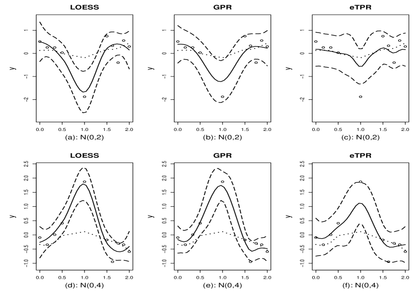
Refer to caption
Figure 6: Predictions in the presence of outlier at the middle data point which is disturbed by additional error generated from $N(0,\sigma^{2})$, where circles represent the observed data, dotted line is the true function, and solid and dashed lines stand for predicted curves and their 95% point-wise confidence intervals from the LOESS, GPR and eTPR methods respectively.
Refer to caption
Figure 7: Predictions in the presence of sparse and outlier at middle point 1.0 which is disturbed by additional error generated from $N(0,\sigma^{2})$, where circles represent the observed data, dotted line is the true function, and solid and dashed lines stand for predicted curves and their 95% point-wise confidence intervals from the LOESS, GPR and eTPR methods respectively.

Two data sets with $m=1$ and sample size of $n_{1}=10$ are generated, where the first $n_{1}-1$ data points $\{x_{1j}\}$ are evenly spaced in [0, 1.5] and the remaining point is at 2.0. At the middle point of $x_{1j}=0.9375$, the observation is added with an extra error from either $N(0,2)$ or $N(0,4)$. Prediction curves, the observed data, the true function and their 95% point-wise confidence intervals, are plotted in Figure 6. We see that the predictions from eTPR shrinks heavily in the area near the data point 1.0, compared to LOESS and GPR.

In addition, we make the data sparse in the area near the point 1.0 by generating the first $4$ and the last $5$ data points $\{x_{1j}\}$ evenly spaced in [0, 0.5] and [1.5, 2.0], respectively, and to make it outlier by adding an extra error from either $N(0,2)$ or $N(0,4)$. Other setups are the same as those in Figure 1. Results are presented in Figure 7. It shows that the predictions from eTPR also shrinks heavily and have more robustness around the data point 1.0, compared with LOESS and GPR.

Table 11: Mean squared errors of prediction results and their standard deviation (in parentheses) by the LOESS, GPR and eTPR methods with $n=60$ and 100.
n Model LOESS GPR eTPR
60 (1) 0.124(0.806) 0.025(0.063) 0.019(0.042)
(2) 0.127(0.803) 0.032(0.079) 0.028(0.076)
(3) 0.063(0.171) 0.036(0.046) 0.032(0.042)
(4) 0.066(0.172) 0.048(0.061) 0.045(0.071)
(5) 0.101(0.550) 0.032(0.086) 0.027(0.060)
(6) 0.346(1.016) 0.264(0.551) 0.268(0.598)
100 (1) 0.152(1.978) 0.017(0.059) 0.013(0.036)
(2) 0.156(1.980) 0.024(0.082) 0.022(0.071)
(3) 0.038(0.102) 0.026(0.032) 0.023(0.025)
(4) 0.041(0.103) 0.036(0.040) 0.033(0.035)
(5) 0.174(2.220) 0.018(0.049) 0.015(0.027)
(6) 0.274(0.719) 0.215(0.349) 0.211(0.346)

To illustrate performance of eTPR with large sample size, data $y_{1j}$ with $n=60$ and 100 are generated from the 6 process models in part (i) in Subsection 5.1. Other setups are the same as those in Table 3, where $N=100$ (150)111100 or 150?. From Table 11, we see that the eTPR method performs better or comparable with GPR, and both are better than LOESS. Combined with the results shown in Table 3, eTPR performs overall better than GPR, but the performance tends to similar when the sample size increases. This matches the theory presented in Proposition 1 that the extended T-process behaves similar to Gaussian process when sample size $n$ is large.

Acknowledgements

Wang’s work is supported by funds of the State Key Program of National Natural Science of China (No. 11231010) and National Natural Science of China (No. 11471302).

References

  • Archambeau and Bach (2010) Archambeau, C. and Bach, F. (2010). Multiple Gaussian Process Models. Advances in Neural Information Processing Systems.
  • Arellano-Valle and Bolfarine (1995) Arellano-Valle, R. B. and Bolfarine, H. (1995). On some characterization of the t-distribution. Statistics & Probability Letters, 25, 79 - 85.
  • Cleveland and Devlin (1988) Cleveland, W.S. and Devlin, S.J. (1988). Locally-Weighted Regression: An Approach to Regression Analysis by Local Fitting. Journal of the American Statistical Association, 83, 596-610.
  • Dutta and Mondal (2015) Dutta, S. and Mondal, D. (2015). An h-likelihood method for spatial mixed linear models based on intrinsic auto-regressions. Journal of the Royal Statistical Society, Ser. B, 77, 699-726.
  • Hall et al. (2008) Hall, P., Müller, H.-G., and Yao, F. (2008). Modelling Sparse Generalized Longitudinal Observations with Latent Gaussian Processes,Journal of Royal Statistical Society, Ser. B, 70, 703-723.
  • Hampel et al. (1986) Hampel, F.R., Ronchetti, E.M., Rousseeuw, P.J. and Stahel, W.A. (1986), Robust Statistics: The Approach Based on Influence Functions, Wiley.
  • Lange et al. (1989) Lange, K.L., Little, R. J.A. and Taylor J. M.G. (1989). Robust statistical modelling using the t distribution, Journal of the American Statistical Association, 84, 881-896.
  • Lee and Kim (2015) Lee, Y. and Kim, G. (2015). H-likelihood predictive intervals for unobservables, International Statistical Review, DOI: 10.1111/insr.12115.
  • Lee and Nelder (1996) Lee, Y. and Nelder, J.A. (1996). Hierarchical Generalized Linear Models. Journal of the Royal Statistical Society B, 58, 619-678.
  • Lee and Nelder (2006) Lee, Y. and Nelder, J.A. (2006). Double hierarchical generalized linear models (with discussion). Journal of the Royal Statistical Society: C (Applied Statistics), 55, 139-185.
  • Lee et al. (2006) Lee, Y., Nelder, J.A. and Pawitan, Y. (2006). Generalized Linear Models with Random Effects, Unified Analysis via H-likelihood. Chapman & Hall/CRC.
  • Ma and Jorgensen (2007) Ma, R. and Jorgensen, B. (2007). Nested generalized linear mixed models: an orthodox best linear unbiased predictor approach. Journal of the Royal Statistical Society, Ser. B, 69, 625-641.
  • Rasmussen and Williams (2006) Rasmussen, C. E. and Williams, C. K. I. (2006). Gaussian Processes for Machine Learning. Cambridge, Massachusetts: The MIT Press.
  • Robinson (1991) Robinson, G.K. (1991). That BLUP is a good thing: the estimation of random effects (with discussion). Statistical Science, 6, 15-51.
  • Sawant et al. (2012) Sawant, P. Billor, N. and Shin, H. (2012) Functional outlier detection with robust func-tional principal component analysis. Computational Statistics, 27, 83 - 102.
  • Seeger et al. (2008) Seeger M. W., Kakade S. M. and Foster D. P. (2008). Information Consistency of Nonparametric Gaussian Process Methods, IEEE Transactions on Information Theory, 54, 2376-2382.
  • Shah et al. (2014) Shah A., Wilson A.G. and Ghahramani Z. (2014). Student-t processes as alternatives to Gaussian processes. Proceedings of the 17th International Conference on Artificial Intelligence and Statistics (AISTATS), 877-885.
  • Shi and Choi (2011) Shi, J. Q. and Choi, T. (2011). Gaussian Process Regression Analysis for Functional Data, London: Chapman and Hall/CRC.
  • Wang and Shi (2014) Wang, B. and Shi, J.Q. (2014). Generalized Gaussian process regression model for non-Gaussian functional data. Journal of the American Statistical Association, 109, 1123-1133.
  • Wauthier and Jordan (2010) Wauthier, F. L. and Jordan, M. I. (2010). Heavy-tailed process priors for selective shrinkage. In Advances in Neural Information Processing Systems, 2406-2414.
  • Xu et al. (2015) Xu, P, Lee, Y. and Shi, J. Q. (2015). Automatic Detection of Significant Areas for Functional Data with Directional Error Control. arXiv:1504.08164.
  • Xu et al. (2011) Xu, Z., Yan, F. and Qi, Y. (2011). Sparse Matrix-Variate t Process Blockmodel. Proceedings of the 25th AAAI Conference on Artificial Intelligence, 543-548.
  • Yu et al. (2007) Yu S., Tresp V. and Yu K. (2007). Robust multi-tast learning with t-process. Proceedings of the 24th International Conference on Machine Learning, 1103-1110.
  • Zellener (1976) Zellener, A. (1976). Bayesian and non-Bayesian analysis of the regression model with multivariate student-t error terms, Journal of the American Statistical Association, 71, 400-405.
  • Zhang and Yeung (2010) Zhang, Y. and Yeung, D.Y. (2010). Multi-task learning using generalized $t$ process. Proceedings of the 13th International Conference on Artificial Intelligence and Statistics (AISTATS), 964-971.
  • Zhou and Stephens (2012) Zhou, X. and Stephens, M. (2012). Genome-wide efficient mixed-model analysis for association studies. Nature Genetics, 44, 821-824.