Instability of Dirac semimetal phase under strong magnetic field

Abstract

The quantum limit can be easily reached in the Dirac semimetals under the magnetic field, which will lead to some exotic many-body physics due to the high degeneracy of the topological zeroth Landau bands (LBs). By solving the effective Hamiltonian, which is derived by tracing out the high energy degrees of freedom, at the self-consistent mean field level, we have systematically studied the instability of Dirac semimetal under a strong magnetic field. A charge density wave (CDW) phase and a polarized nematic phase formed by “exciton condensation” are predicted as the ground state for the tilted and untilted bands, respectively. Furthermore, we propose that, distinguished from the CDW phase, the nematic phase can be identified in experiments by anisotropic transport and Raman scattering.

I Introduction

Searching for new states of matter in solid materials is one of the key problems in condensed matter physics, which attracts lots of research interests recently. External magnetic field has provided an additional dimension for such studies, leading to surprisingly rich phenomenons and phases in two dimensional electron gas systems already, e.g. the integer Klitzing et al. (1980) and fractional Tsui et al. (1982) quantum Hall effects, the Wigner crystal phase as well as the nematic phases Lilly et al. (1999); Du1 (1999); Feldman et al. (2016). The high degeneracy of Landau levels resulted from the Landau quantization of the electronic wave functions is the main origin of the instability towards the various exotic phases mentioned above. In three dimensional systems, the Landau quantization only happens in the plane perpendicular to the magnetic field and the energy dispersion along the field direction remains unchanged. For ordinary semiconductor system with quadratic band dispersion, the high degeneracy of the LBs leads to almost perfect nesting of the “Fermi surfaces” along the field direction, as illustrated schematically in Fig. (1). Such a nesting effect will be greatly enhanced in the so called quantum limit, where only the lowest LB cuts through the Fermi level, and the field induced symmetry breaking phases such as CDW Celli and Mermin (1965); Iye et al. (1984); Alicea and Balents (2009), spin-density wave Celli and Mermin (1965); noa (1987); Tesanovi? and Halperin (1987), valley-density wave Tesanovi? and Halperin (1987), will be stabilized as the ground state.

It is very difficult to reach the quantum limit in normal semiconductors and semimetals and the experimental observation of the field induced CDW phase in real materials, i.e. Bi and Sb, is still under debate. Behnia et al. (2007); Li et al. (2008) The recently discovered topological semimetals provide a new platform for the search of new exotic phenomenons under magnetic field. Nielsen and Ninomiya (1983); Son and Spivak (2013); Burkov (2014); Parameswaran et al. (2014); Xiong et al. (2015); Lu and Shen (2015); Song et al. (2016); Rinkel et al. (2016); Zhang et al. (2015) For Dirac Young et al. (2012); Wang et al. (2012); Yang and Nagaosa (2014) or Weyl Burkov and Balents (2011); Wan et al. (2011); Weng et al. (2015); Huang et al. (2015); Lv et al. (2015); Xu et al. (2015a); Nie et al. (2017) semimetals, where the Fermi level is very close to the Dirac or Weyl points, the quantum limit can be easily reached even under a weak magnetic field and more fruitful many-body physics can be realized due to the extra valley and orbital degrees of freedom. Miransky and Shovkovy (2015); Shovkovy (2013) For instance, in strong magnetic field, the Weyl semimetal is found to be stabilized as a chiral-symmetry-breaking CDW state. Roy and Sau (2015); Zhang and Shindou (2017) In the present Letter, we systematically study the possible instabilities of Dirac semimetal state under the magnetic field in the quantum limit. We find that, besides the CDW phase, a new state, the polarized nematic phase can be stabilized in a large part of the phase diagram. Such an exotic phase is caused by the “exciton condensation” between the two zeroth LBs, which breaks both the rotational symmetry and the inversion symmetry, leading to a number of important physical consequences in transport and optical experiments.

II Model

The Dirac semimetals can be divided into two categories by whether the Dirac points (DPs) are located on high symmetry lines or points Yang and Nagaosa (2014) of the Brillouin zone (BZ). In this Letter, we will focus on the first category, where the DPs are protected by the crystalline symmetry along the high symmetry lines and always appear in pairs due to the presence of the time reversal symmetry. The typical example of such type of materials is $\mathrm{Na_{3}Bi}$ Wang et al. (2012), where the DPs are generated by the crossings of two doubly degenerate bands along the $z$ axis. The low energy physics of such type of Dirac semimetal can be well described by the following k$\cdot$p model,

$$H^{0}=C(k_{z})+\begin{pmatrix}M\left(k_{z}\right)&-v\hbar k_{-}&\gamma\left(\mathbf{k}\right)&0\\ -v\hbar k_{+}&-M\left(k_{z}\right)&0&\gamma\left(\mathbf{k}\right)\\ \gamma^{*}\left(\mathbf{k}\right)&0&-M\left(k_{z}\right)&v\hbar k_{-}\\ 0&\gamma^{*}\left(\mathbf{k}\right)&v\hbar k_{+}&M\left(k_{z}\right)\end{pmatrix}$$ (1)

Here $C(k_{z})=C_{0}(\cos a_{0}k_{z}-\cos a_{0}k_{c})$, $M\left(k_{z}\right)=M_{0}\left(\cos a_{0}k_{z}-\cos a_{0}k_{c}\right)$, $k_{\pm}=k_{x}\pm ik_{y}$, $v$ is the velocity in $xy$ plane, $a_{0}$ is the lattice along $k_{z}$, and $\pm k_{c}$ are the locations of DPs. The bases of the k$\cdot$p model can be labeled by their main orbital characters as $\left|P\frac{3}{2}\right\rangle$, $\left|S\frac{1}{2}\right\rangle$, $\left|S-\frac{1}{2}\right\rangle$, $\left|P-\frac{3}{2}\right\rangle$, respectively. The first term in Eq. (1) plays an important role in the formation of type II Weyl points. Soluyanov et al. (2015); Xu et al. (2015b) While as long as $|C_{0}|<|M_{0}|$, that is the case we focus on, the $C(k_{z})$ term will just tilt the DPs and change the ellipsoidal Fermi surface to a pyriform one. Even so, as shown in the following, this term will play an important role in determining whether the CDW or nematic phase will be stabilized. The high order term $\gamma(\mathbf{k})$ won’t play any important role for the physics discussed here and so will be neglected in the rest of the Letter.

The external magnetic field $B$ is applied along the $z$ direction. Adopt the Landau gauge $\mathbf{A}=\left(-yB,0,0\right)$, which leaves $k_{x}$ and $k_{z}$ still good quantum numbers, the LB eigenenergies and eigenstates can be solved analytically (see appendix A). As shown in Fig. (1), the two zeroth LBs disperse linearly and cross with each other at the DPs. The quantum limit can be reached by increasing the magnetic field such that only the zeroth LBs cuts through the Fermi level. In the present work we are only interested in the instability in the quantum limit, therefore we only keep the zeroth LBs in the non-interacting Hamiltonian

$$\hat{H}^{0}=\sum_{ak_{x}k_{z}}\epsilon_{k_{z}a}\hat{\psi}_{k_{x}k_{z}a}^{\dagger}\hat{\psi}_{k_{x}k_{z}a}$$ (2)

$$\epsilon_{k_{z}a}=\begin{cases}C(k_{z})-M\left(k_{z}\right)&a=c\\ C(k_{z})+M\left(k_{z}\right)&a=v\end{cases}$$ (3)

Here $c$ and $v$ represent the conduction band (red band in Fig. (1)) and valence band (blue band in Fig. (1)), which are formed by $\left|S\frac{1}{2}\right\rangle$ and $\left|P-\frac{3}{2}\right\rangle$ states respectively. Since they belong to different eigenvalues of $C_{6}$, the crossings at $\pm k_{c}$ are protected by rotational symmetry and will persist even if nonzero $\gamma\left(\mathbf{k}\right)$ presents.

Notice that the Zeeman’s coupling between the magnetic field and the field-free orbitals is neglected here. In a first principle study of the effective g factor, gfa we show that the Zeeman’s splitting in a typical Dirac semimetal under magnetic field as strong as 100T is just about 5meV, which is much smaller than the band inversion energy ($M_{0}$) and so would not affect the discussion qualitatively.

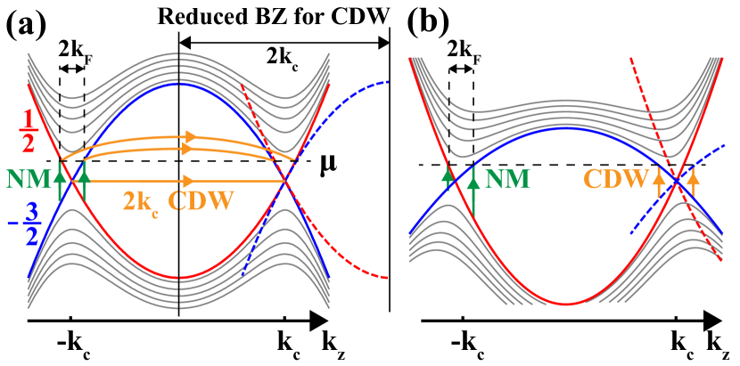
Figure 1: Band structure and instability channels. The two zeroth LBs, referred as the conductance and valence bands, are plotted in red and blue respectively, and the high energy LBs are plotted in gray. (a) shows the nematic phase channel (green arrows) and three CDW phase channels (orange arrows) in an untilted band structure ($C_{0}=0$). As argued in the text, only the nematic phase and the $2k_{c}$ CDW phase can be realized in low density limit. Here the dashed colored lines represent the folded bands in the $2k_{c}$ CDW phase. (b) shows the two channels in a tilted band structure ($C_{0}\neq 0$). It is apparent that the kinetic energy cost of the $2k_{c}$ CDW order will be significantly lowered by the tilting.

III Effective interaction

To explore the stability of the above system under Coulomb repulsive interaction, we need to derive an effective interaction for the zeroth LBs by tracing out all the high LBs. Take the random phase approximation (RPA), we get

$$\hat{H}_{\mathrm{int}}^{\mathrm{eff}} =\frac{1}{2\Omega}\sum_{\mathbf{q}\neq 0}\sum_{k_{x}k_{z}}\sum_{p_{x}p_{z}}\sum_{ab}e^{il_{B}^{2}q_{y}\left(k_{x}-p_{x}\right)}W\left(\mathbf{q}\right)$$

$$\times \hat{\psi}_{k_{x}+q_{x,}k_{z}+q_{z},a}^{\dagger}\hat{\psi}_{p_{x},p_{z},b}^{\dagger}\hat{\psi}_{p_{x}+q_{x},p_{z}+q_{z},b}\hat{\psi}_{k_{x},k_{z},a}$$ (4)

$$W\left(\mathbf{q}\right) =\frac{e^{2}}{\epsilon_{0}\kappa\left(\mathbf{q}\right)\mathbf{q}^{2}}e^{-\frac{1}{2}l_{B}^{2}\mathbf{q}_{\perp}^{2}}$$ (5)

where $\mathbf{q}_{\perp}=\left(q_{x},q_{y}\right)$, $l_{B}=\sqrt{\frac{\hbar}{eB}}$ is the magnetic length, $\kappa(\mathbf{q})$ is the effective dielectric function, and $\Omega$ is the sample volume. Details of the RPA derivation and the discussion of the dielectric function are given in appendix B. As shown below, the long wave part of the interaction contributes the most in both of the possible instabilities, thus we can approximate $\kappa\left(\mathbf{q}\right)$ by a dielectric constant $\kappa=\kappa_{0}+\frac{1}{3}\kappa_{z}+\frac{2}{3}\kappa_{xy}$, where

$$\kappa_{z}\approx\frac{e{}^{2}u}{3\pi^{2}\epsilon_{0}v^{2}\hbar}\left(0.9+\ln\left(\frac{M_{0}l_{B}}{v\hbar}\right)\right)$$ (6)

$$\kappa_{xy}\approx\frac{e{}^{2}}{4\pi^{2}\epsilon_{0}u\hbar}\left(0.6+\ln\left(\frac{M_{0}l_{B}}{v\hbar}\right)\right)$$ (7)

are the dielectric constants from high LBs, $\kappa_{0}$ is the dielectric constant from the core electrons, and $u=\frac{1}{\hbar}M_{0}a_{0}\sin\left(a_{0}k_{c}\right)$ is the Dirac velocity along $z$ direction. The derivation of such dielectric constants is given in appendix C. It should be aware that the results in Eq. (6)-(7) are not only applied to this particular model, in fact it is universal for all the Dirac/Weyl semimetals. One of the important features for the above effective interaction is that its strength can be tuned by external magnetic field, which is a bit unusual in condensed matter physics. The mechanism is easy to be understood, that is, the energy gap between the zeroth and high LBs increases with the field strength, which weakens the screening effect.

IV COHSEX method

It is well known that the direct Hartree-Fock mean field approximation for metals with long range Coulomb interaction leads to a singular Fermi velocity because of a logarithmic divergence in the exchange channel. To handle this problem, we adopt the “Coulomb hole plus screened exchange” (COHSEX) method, which is a simplified version of the GW method Hedin (1965). Applying this method to our model, the self energy consists of a direct Hartree term $\Sigma^{\mathrm{H}}$ and a screened exchange term $\Sigma^{\mathrm{E}}$ where the interaction is not only screened by high LB electrons but also the zeroth LB electrons. As explained in the next section, in low carrier density limit, the system has a CDW instability at $Q=2k_{c}$. For convenience of calculation, we take the commensurate limit by setting $k_{c}=\frac{\pi}{D_{c}a_{0}}$, where $D_{c}$ is an integer. The BZ will be folded $D_{c}$ times if the CDW order presents. Thus, in general, we can define the Green’s function as $G_{an,bm}(k_{x},k_{z},t)=\langle T_{t}\hat{\psi}_{k_{x},k_{z}+nQ,a}(t)\hat{\psi}_{k_{x},k_{z}+mQ,b}^{\dagger}(0)\rangle$, where $n,m=0\cdots D_{c}-1$ is the sub-BZ index and $k_{z}$ takes value in the reduced BZ: $0\leq k_{z}<Q$. Then the self energy can be expressed as (Fig. (2b))

$$\Sigma_{an,bm}^{\mathrm{H}}\left(k_{x}k_{z}\right) =\delta_{ab}W\left(0,0,\left(n-m\right)Q\right)\int\frac{dp_{x}dp_{z}d\omega}{\left(2\pi\right)^{3}}$$

$$\times \sum_{cn^{\prime}}G_{c,n^{\prime}+n-m;c,n^{\prime}}\left(p_{x},p_{z},\omega\right)e^{i\omega 0^{+}}$$ (8)

$$\Sigma_{an,bm}^{\mathrm{E}}\left(k_{x}k_{z}\right) =-\sum_{n^{\prime}}\int\frac{d^{2}\mathbf{q}_{\perp}}{\left(2\pi\right)^{2}}\int\frac{dp_{z}d\omega}{\left(2\pi\right)^{2}}$$

$$\times W^{\mathrm{S}}\left(\omega=0,\mathbf{q}_{\perp},k_{z}-p_{z}+n^{\prime}Q\right)$$

$$\times G_{a,n-n^{\prime};b,m-n^{\prime}}\left(k_{x}-q_{x},p_{z},\omega\right)e^{i\omega 0^{+}}$$ (9)

where $W^{\mathrm{S}}(\omega=0)$ is the static screened interaction. Here we approximate the Green’s function screening $W^{\mathrm{S}}$ by the free Green’s function at zero doping, as shown in Fig. (2c). Such an approximated screened interaction can be derived analytically

$$W^{\mathrm{S}}\left(\omega=0,\mathbf{q}\right)=\frac{e^{2}}{\epsilon_{0}}\cdot\frac{e^{-\frac{1}{2}l_{B}^{2}\mathbf{q}_{\perp}^{2}}}{\kappa\mathbf{q}^{2}+q_{\mathrm{TF}}^{2}(q_{z})e^{-\frac{1}{2}l_{B}^{2}\mathbf{q}_{\perp}^{2}}}$$ (10)

where $q_{\mathrm{TF}}(q_{z})$ is the effective Thomas-Fermi wavevector

$$q_{\mathrm{TF}}^{2}(q_{z})=\frac{e^{2}M_{0}\ln\left|\frac{\sin ak_{c}+\sin\frac{aq_{z}}{2}}{\sin ak_{c}-\sin\frac{aq_{z}}{2}}\right|}{2\epsilon_{0}\pi^{2}l_{B}^{2}\left(M_{0}^{2}-C_{0}^{2}\right)a\sin\frac{aq_{z}}{2}}$$ (11)

We have checked this approximation by comparing it with full self-consistent calculations, where $W^{\mathrm{S}}$ is calculated from $G$ self-consistently, and find that the correction on results is very small.

With the above approximation, the Dyson’s equation $({\hat{G}}^{0-1}-{\hat{\Sigma}}){\hat{G}}=\mathbb{I}$ (Fig. (2a)) and the equations (8) and (9) set up a self-consistent loop to determine the possible symmetry breaking phases at zero temperature by assuming different non-diagonal matrix elements in the self energy matrix. For convenience, we define the order parameter as $\Delta_{an,bm}(k_{x},k_{z})=\langle\psi^{\dagger}_{an}(k_{x},k_{z})\psi_{bm}(k_{x},k_{z})\rangle$, whose non-diagonal elements in the band index $a,b$ and sub-BZ index $n,m$ denote the appearance of the nematic phase and the CDW phase respectively.

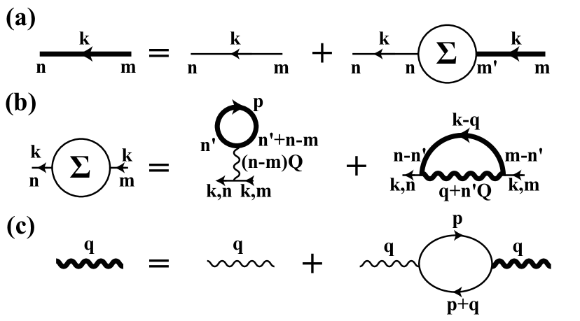
Figure 2: Feynman diagrams for the COHSEX method. The full and free Green’s functions are represented by thick and thin lines, respectively. Correspondingly, the screened effective interaction $W^{\mathrm{S}}$ and the bare effective interaction $W$ are represented by thick and thin wavy lines, respectively. (a) is the diagram for the Dyson’s equation. (b) is the diagram for the self energy. (c) is the diagram for the screened effective interaction, where the Green’s functions participating the screening are approximated by the free Green’s functions.

V CDW phase

CDW phase acquires its instability from the Fermi surface nesting in the quasi one dimensional band structure (Fig. (1)). At first sight, it seems that the CDW should occur simultaneously at $Q=2k_{c}+2k_{F}$ and $Q=2k_{c}-2k_{F}$ channels for conduction and valence bands respectively. However, the interband Hartree energy can lock the CDWs in different bands to same $Q=2k_{c}$ at least for low enough carrier density. This conclusion can be reached by simply comparing the energy difference between the CDW phases with $Q=2k_{c}\pm 2k_{F}$ and $Q=2k_{c}$. According to Eq. (8), the $Q=2k_{c}$ phase gains an extra interband Hartree energy of $\sim W\left(Q\right)\Re e(\Delta_{c0,c-1}^{\mathrm{CDW}}\Delta_{v0,v-1}^{\mathrm{CDW*}})$, which reaches a negative constant as $k_{F}$ approaching zero if $\Delta_{c0,c-1}^{\mathrm{CDW}}=-\Delta_{v0,v-1}^{\mathrm{CDW}}$. While the kinetic energy and exchange energy (Eq. (9)) difference between the $Q=2k_{c}$ and the $Q=2k_{c}\pm 2k_{F}$ phases will vanish with $k_{F}$ approaching zero. Therefore as long as $k_{F}$ is small enough, the CDW phase with $Q=2k_{c}$ for both bands will be stabilized.

The numerical calculation is performed with the initial condition $\Delta_{an,bm}^{\mathrm{CDW}}(k_{x},k_{z})=\delta_{n,m+1}\eta_{a,b}(k_{z})+\delta_{n+1,m}\eta_{b,a}^{*}(k_{z})$, where $\eta(k_{z})$ is a random matrix. The parameters are set as $\kappa_{0}=5$, $a_{0}=9.66\mathrm{\mathring{A}}$, $M_{0}a_{0}=2.3\mathrm{eV\cdot\mathrm{\mathring{A}}}$, $\hbar v=2.0\mathrm{eV\cdot\mathring{A}}$ and $D_{c}=4$, which give the same Dirac velocity for Na₃Bi with the first principle results. Wang et al. (2012) We set $C_{0}$ as $C_{0}=-tM_{0}$, where $t\in[0,1)$ is the tilting ratio describing how much the bands are tilted. In Fig. (3b), we plot the band gaps and order parameters at various tilting ratios and magnetic fields. It shows that the tilting can significantly enlarge the CDW order, which is a direct consequence of saving the kinetic energy, as sketched in Fig. (1b).

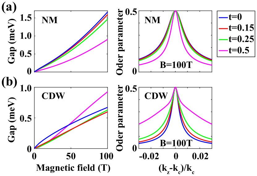
Figure 3: In the left panel, the energy gaps of the polarized nematic and CDW phases at zero doping and a few tilting ratios are plotted as functions of magnetic field. In the right panel, the corresponding order parameters of the two phases at $B=100\mathrm{T}$, i.e. $|\Delta_{v;c}^{\mathrm{NM}}(k_{z})|$ and $\sqrt{\sum_{a}|\Delta_{a,-1;a,0}^{\mathrm{CDW}}|^{2}}$, are plotted around the DPs.

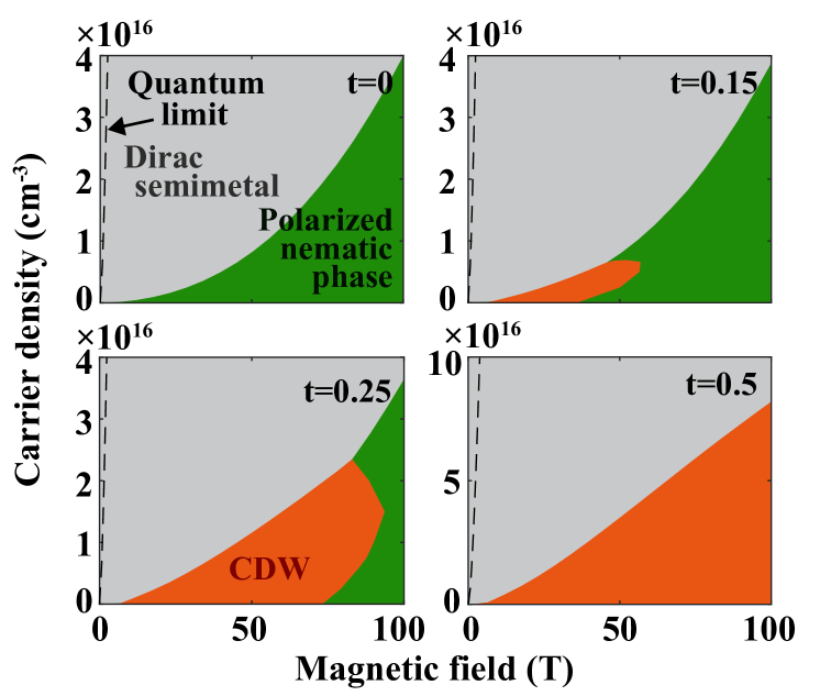
Figure 4: The phase diagram in density-field parameter space at a few tilting ratios. Here the critical field to achieve the quantum limit are indicated by dashed lines, and, the Dirac semimetal, polarized nematic, and CDW phases are represented by gray, green, and orange areas, respectively. It shows that the polarized nematic phase is more favoured in untilted bands, while the CDW phase is more favoured in tilted bands.

VI Nematic phase

As shown in Fig. (1), if the chemical potential is close enough to the DPs a rotation broken phase, i.e. the nematic phase, can be stabilized. Since the nematic phase doesn’t break the translational symmetry, its order parameter can be expressed in the full BZ as $\Delta_{a,b}^{\mathrm{NM}}(k_{x},k_{z})=\delta_{\bar{a}b}\eta(k_{z})$, where $-\pi\leq k_{z}<\pi$, and $\bar{a}=v(c)$ for $a=c(v)$. Two different types of $\eta$ can be got: odd or even with respect to $k_{z}$. According to the definition of LB wave function sup , inversion operator acts on it as

$$\mathcal{P}\hat{\psi}_{k_{x},k_{z},c}^{\dagger}\hat{\psi}_{k_{x},k_{z},v}\mathcal{P}^{-1}=-\hat{\psi}_{-k_{x},-k_{z},c}^{\dagger}\hat{\psi}_{-k_{x},-k_{z},v}$$ (12)

, thus the even and odd $\eta$ will respectively break and maintain the inversion symmetry. As will be discussed in the next paragraph, the inversion broken phase, which will be referred as the polarized nematic phase in the following, is always more favored.

The band gaps and order parameters of the polarized nematic phase, and the phase diagram consisting of the phases mentioned above are calculated with the same parameters used for the CDW phase and shown in Fig. (3a) and (4) respectively, which indicates that the polarized nematic phase is more favoured in untilted bands while the CDW phase is more favoured in tilted bands. This can be understood as a result of competition between kinetic energy and interaction energy. One one hand, as will be explained latter, the polarized nematic phase has a lower interaction energy; on the other hand, as shown in Fig. (1b), the tilting will significantly lower the kinetic energy cost in the CDW phase. Therefore, as shown in Fig. (4), the area of the polarized nematic phase in phase diagram will shrink and eventually vanish with an increasing tilting. Now let us explain why the polarized nematic phase has a lower interaction energy. Since its Hartree energy reaches zero, i.e. the minimum, we only need to compare the exchange energies. Eq. (9) suggests that the exchange energy in the CDW phase is approximately $-W^{\mathrm{S}}(\mathbf{q}_{\perp},0)|\Delta_{a,0;a,-1}^{\mathrm{CDW}}|^{2}$. While the exchange energy in the nematic phase consists of three parts: two intravalley parts $-\frac{1}{2}W^{\mathrm{S}}(\mathbf{q}_{\perp},0)|\Delta_{a\bar{a}}^{\mathrm{NM}}(\pm k_{c})|^{2}$, which equal to the CDW one; and an intervalley part $-W^{\mathrm{S}}(\mathbf{q}_{\perp},Q)\Re e(\Delta_{a\bar{a}}^{\mathrm{NM}}(k_{c})\Delta_{a\bar{a}}^{\mathrm{NM*}}(-k_{c}))$, which is negative in the polarized nematic phase ($\Delta_{a\bar{a}}^{\mathrm{NM}}(k_{c})=\Delta_{a\bar{a}}^{\mathrm{NM}}(-k_{c})$). Here we have omitted the summation and integral symbols for brevity. Thus we conclude that the polarized nematic order has lower interaction energy than the inversion symmetric nematic order and the CDW order.

Another aspect to understand this nematic order is to view it as a “pairing order” between electrons in the conduction band and holes in the valence band, which is the “exciton condensation” state in the mean field level. Lerner and Lozovik (1980) Formally we can rewrite the creation operators of electrons and holes as $\psi_{k_{x},k_{z},c}^{\dagger}=\psi_{k_{x},k_{z}}^{\mathrm{e}\dagger}$, $\psi_{k_{x},k_{z},v}=\psi_{-k_{x},-k_{z}}^{\mathrm{h}\dagger}$, and rewrite the order parameter as a pairing order $\langle\psi_{k_{x},k_{z}}^{\mathrm{e}\dagger}\psi_{-k_{x},-k_{z}}^{\mathrm{h}\dagger}\rangle$. Then the exchange interaction turns into an effective attractive interaction between the electrons in the conduction band and holes in the valence band. And our mean field theory is equivalent to the BCS theory for superconductivity. Since the system is three dimensional, the quantum fluctuation and disorder can not suppress the phase coherence completely and such a transition can survive even beyond the mean field approximation.

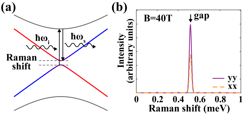
Figure 5: Raman scattering characterizing the nematic phase. In (a) the scattering process that reveals the rotation symmetry breaking is sketched. In (b) the numerical differential scattering section at zero doping and $B=40\mathrm{T}$ is shown.

VII Experimental aspects

The most direct consequence of both the nematic and CDW phase transitions is the opening of an energy gap between the zeroth LBs, which can be observed easily through the transport measurement. For the CDW phase, since the order wave-vector given by the distance between two DPs is in general incommensurate with the lattice, the corresponding Goldstone mode, i.e. the so called sliding mode, will contribute to an electric field dependent conductivity along the wave-vector direction due to the depinning effect. Lee and Rice (1979) While, for the nematic phase, an anisotropic resistance in the $xy$ plane is expected due to the rotational symmetry breaking. Since the original rotational symmetry is discrete, the corresponding Goldstone mode in the nematic phase will be gapped and can de detected by neutron scattering experiments.

Another evidence for the nematic phase should be the anisotropy in the inelastic light scattering shown in Fig. (5a), where a strongly anisotropic scattering section with a Raman shift of the band gap will be observed, since both the initial and final states are rotation broken. To verify this, we apply a numerical study of the Raman scattering section with the formula $\frac{\partial^{2}\sigma}{\partial\Omega\partial\omega_{s}}\propto\sum_{F}\left|M_{F,G}\right|^{2}\delta\left(E_{F}-E_{I}-\hbar\Omega\right)$ where $\Omega=\omega_{i}-\omega_{s}$ is the Raman shift and $M_{F,I}$ is the light scattering matrix element Devereaux and Hackl (2007):

$$M_{F,I} =\mathbf{e}_{i}\cdot\mathbf{e}_{s}\left\langle F\right|\hat{\rho}\left|G\right\rangle$$

$$+ \frac{1}{m}\sum_{J}\left[\frac{\left\langle F\right|\hat{\pi}^{s}\left|J\right\rangle\left\langle J\right|\hat{\pi}^{i}\left|G\right\rangle}{E_{G}-E_{J}+\omega_{i}}+\frac{\left\langle F\right|\hat{\pi}^{i}\left|J\right\rangle\left\langle J\right|\hat{\pi}^{s}\left|G\right\rangle}{E_{G}-E_{J}-\omega_{s}}\right]$$ (13)

Here $\left|G\right\rangle$, $\left|J\right\rangle$ and $\left|F\right\rangle$ represent the initial (ground), intermediate and final many body states having energies $E_{G,J,F}$, respectively. $i,s$ represent the polarization direction of the initial and scattered photons, respectively. And, $\hat{\rho}$, $\hat{\pi}$ are the density and velocity operators in second quantization form, respectively. Results at zero doping and field $B=40\mathrm{T}$ is shown in Fig. (5b), where the large splitting in the $xx$ and $yy$ polarized light measurements indicates the rotation symmetry breaking.

VIII Summary

In summary, we have systematically studied the instabilities of Dirac semimetal phase in the quantum limit due to the Coulomb interaction. The high LB electrons far away from the Fermi level are considered as a background to screen the interaction by an effective dielectric constant in the long wavelength limit. All the possible instabilities on the zeroth LBs, i.e. the inter/intra-valley and inter/intra-band channels, are treated within the so called COHSEX method. By numerical calculations, we have shown that a polarized nematic phase breaking both the rotational and inversion symmetry and a CDW phase breaking translational symmetry will be stabilized depending on the strength of the tilting terms for the Dirac cones. Relevant experiments, including transport and Raman scattering, are also proposed to verify the existence of such phases. Further theoretical studies on the physical properties like magneto-transport in these exotic phases are also strongly encouraged.

Appendix A Solution of the free Hamiltonian

The eigenenergies and eigenstates of our model Hamiltonian can be explicitly derived as Abrikosov (1998)

$$\epsilon_{k_{z}s\alpha}=\begin{cases}C(k_{z})+\sqrt{M^{2}\left(k_{z}\right)+2\hbar^{2}v^{2}l_{B}^{-2}\left|\alpha\right|}&\alpha>0\\ C(k_{z})-sM\left(k_{z}\right)&\alpha=0\\ C(k_{z})-\sqrt{M^{2}\left(k_{z}\right)+2\hbar^{2}v^{2}l_{B}^{-2}\left|\alpha\right|}&\alpha<0\end{cases}$$ (14)

$$\hat{\psi}_{k_{x}k_{z}s\alpha}^{\dagger} =\frac{1}{\sqrt{l_{z}l_{x}}}\sum_{j_{z}}\delta_{s,\mathrm{sign}(j_{z})}C_{j_{z}}^{k_{z}s\alpha}$$

$$\times \int d^{3}\mathbf{r}e^{i\left(k_{z}z+k_{x}x\right)}H_{\alpha^{\prime}}\left(\frac{y}{l_{B}}-l_{B}k_{x}\right)\hat{\psi}_{j_{z}}^{\dagger}\left(\mathbf{r}\right)$$ (15)

, where $s=1(-1)$ represents the left up (right down) block in the Hamiltonian, $\alpha=$$0,\pm 1,\cdots$ is the LB index, $j_{z}=\frac{3}{2},\frac{1}{2},-\frac{1}{2},-\frac{3}{2}$ is the k$\cdot$p basis index, and $H_{\alpha^{\prime}}$ is the $\alpha^{\prime}$-th order one-dimensional harmonic oscillator. Here $\alpha^{\prime}$ is defined as $\alpha^{\prime}=|\alpha|+s-j_{z}-\frac{1}{2}$, which equals to $|\alpha|-1,|\alpha|,|\alpha|-1,|\alpha|$ for $j_{z}=\frac{3}{2},\frac{1}{2},-\frac{1}{2},-\frac{3}{2}$ respectively, and $\alpha^{\prime}=-1$ terms should be omitted. The coefficient $C_{j_{z}}^{k_{z}s\alpha}$ is defined as

$$C_{\frac{3}{2}}^{k_{z},+1,\alpha} =\cos\frac{\theta}{2}\qquad C_{\frac{1}{2}}^{k_{z},+1,\alpha}=\sin\frac{\theta}{2}$$

$$C_{-\frac{1}{2}}^{k_{z},-1,\alpha} =-\sin\frac{\theta}{2}\qquad C_{-\frac{3}{2}}^{k_{z},-1,\alpha}=\cos\frac{\theta}{2}$$ (16)

for $\alpha>0$,

$$C_{\frac{3}{2}}^{k_{z},+1,\alpha} =-\sin\frac{\theta}{2}\qquad C_{\frac{1}{2}}^{k_{z},+1,\alpha}=\cos\frac{\theta}{2}$$

$$C_{-\frac{1}{2}}^{k_{z},-1,\alpha} =\cos\frac{\theta}{2}\qquad C_{-\frac{3}{2}}^{k_{z},-1,\alpha}=\sin\frac{\theta}{2}$$ (17)

for $\alpha<0$, and

$$C_{\frac{3}{2}}^{k_{z},+1,\alpha} =0\qquad C_{\frac{1}{2}}^{k_{z},+1,\alpha}=1$$

$$C_{-\frac{1}{2}}^{k_{z},-1,\alpha} =0\qquad C_{-\frac{3}{2}}^{k_{z},-1,\alpha}=1$$ (18)

for $\alpha=0$, respectively, where the auxiliary angle $\theta$ is set by $\theta=\arctan\frac{v\hbar\sqrt{2|\alpha|}}{M(k_{z})l_{B}}$ ($0\leq\theta<\pi$).

The conduction and valence bands in the paper are the $\alpha=0,s=1$ and $\alpha=0,s=-1$ bands here.

Appendix B Effective interaction on the zeroth LBs

In this section, we will derive the effective interaction on the zeroth LBs by tracing out the high LBs in RPA. The long range Coulomb interaction can be written as

$$\hat{H}_{\mathrm{int}} =\frac{1}{2}\sum_{j_{z}j_{z}^{\prime}}\int d^{3}\mathbf{r}\int d^{3}\mathbf{r}^{\prime}\frac{e^{2}}{4\pi\epsilon_{0}\kappa_{0}\left|\mathbf{r}-\mathbf{r}^{\prime}\right|}$$

$$\times\hat{\psi}_{j_{z}}^{\dagger}\left(\mathbf{r}\right)\hat{\psi}_{j_{z}^{\prime}}^{\dagger}\left(\mathbf{r}^{\prime}\right)\hat{\psi}_{j_{z}^{\prime}}\left(\mathbf{r}^{\prime}\right)\hat{\psi}_{j_{z}}\left(\mathbf{r}\right)$$ (19)

where $\kappa_{0}$ is the dielectric constant contributed by the core electron states. By a representation transformation, the interaction can be written on the LB bases

$$\hat{H}_{\mathrm{int}} =\frac{1}{2\Omega}\sum_{\mathbf{q}\neq 0}\sum_{k_{x}k_{z}}\sum_{p_{x}p_{z}}\sum_{ss^{\prime}}\sum_{\alpha\beta\alpha^{\prime}\beta^{\prime}}e^{il_{B}^{2}q_{y}\left(k_{x}-p_{x}\right)}$$

$$\times U_{k_{z}s\alpha\alpha^{\prime},p_{z}s^{\prime}\beta\beta^{\prime}}\left(\mathbf{q}\right)\hat{\psi}_{k_{x}+q_{x},k_{z}+q_{z},s\alpha^{\prime}}^{\dagger}\hat{\psi}_{p_{x},p_{z},s^{\prime}\beta}^{\dagger}$$

$$\times\hat{\psi}_{p_{x}+q_{x},p_{z}+q_{z},s^{\prime}\beta^{\prime}}\hat{\psi}_{k_{x},k_{z},s\alpha}$$ (20)

where

$$U_{k_{z}s\alpha\alpha^{\prime},p_{z}s^{\prime}\beta\beta^{\prime}}\left(\mathbf{q}\right) =\frac{e^{2}}{\epsilon_{0}\kappa_{0}\mathbf{q}^{2}}e^{-\frac{1}{2}l_{B}^{2}\mathbf{q}_{\perp}^{2}}$$

$$\times\Lambda_{k_{z}s\alpha\alpha^{\prime}}^{*}\left(\mathbf{q}\right)\Lambda_{p_{z}s^{\prime}\beta\beta^{\prime}}\left(\mathbf{q}\right)$$ (21)

$$\Lambda_{p_{z}s^{\prime}\beta\beta^{\prime}}\left(\mathbf{q}\right)=\sum_{j_{z}}\delta_{s^{\prime},\mathrm{sign}(j_{z})}C_{j_{z}}^{p_{z}s^{\prime}\beta*}C_{j_{z}}^{p_{z}+q_{z},s^{\prime}\beta^{\prime}}$$

$$\quad\times F_{\left|\beta\right|+s^{\prime}-j_{z}-\frac{1}{2},\left|\beta^{\prime}\right|+s^{\prime}-j_{z}-\frac{1}{2}}\left(\frac{l_{B}\left(q_{x}-iq_{y}\right)}{\sqrt{2}}\right)$$ (22)

Here $F_{\alpha,\beta}\left(\xi\right)$ is the well known form factor of Landau levels, which is defined as

$$F_{\alpha,\beta}\left(\xi\right)=\sqrt{\frac{\beta!}{\alpha!}}\xi^{\alpha-\beta}L_{\beta}^{\left(\alpha-\beta\right)}\left(\left|\xi\right|^{2}\right)$$ (23)

for $\alpha\geq\beta$ and $F_{\alpha,\beta}\left(\xi\right)=F_{\beta,\alpha}^{*}\left(-\xi\right)$ for $\alpha\leq\beta$ , and $L_{\beta}^{\left(\alpha-\beta\right)}$ is the Laguerre polynomial MacDonald (1994); Cahill and Glauber (1969).

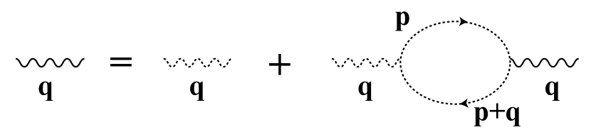
Figure 6: RPA diagrams of the effective interaction on the zeroth LBs. The solid wavy line represents the effective interaction, while the dashed wavy line represents the bare interaction. The dashed straight line represents the Green’s functions in high LBs.

In the Feynman’s diagram representation, the RPA effective interaction on the zeroth LBs can be interpreted as the “dressed” interaction, that has been inserted with bubble diagrams concerning high LBs (Fig. (6)). Thus the static effective interaction satisfy

$$W\left(\mathbf{q}\right)=U\left(\mathbf{q}\right)+U\left(\mathbf{q}\right)\chi^{0>}\left(0q_{x}q_{z}\right)W\left(\mathbf{q}\right)$$ (24)

, where the matrix subscripts are omitted. $\chi^{0>}$ is the bare susceptibility of high LBs:

$$\chi_{k_{x}k_{z}s\alpha\beta,k_{x}^{\prime}k_{z}^{\prime}s^{\prime}\alpha^{\prime}\beta^{\prime}}^{0>}\left(\omega q_{x}q_{z}\right)=\delta_{k_{x}k_{x}^{\prime}}\delta_{k_{z}k_{z}^{\prime}}\delta_{ss^{\prime}}\delta_{\alpha\alpha^{\prime}}\delta_{\beta\beta^{\prime}}$$

$$\times\frac{1}{\Omega}\begin{cases}\frac{n_{F}\left(\epsilon_{k_{z}s\alpha}-\mu\right)-n_{F}\left(\epsilon_{k_{z}+q_{z}s\beta}-\mu\right)}{\omega+\epsilon_{k_{z}s\alpha}-\epsilon_{k_{z}+q_{z}s\beta}}&\alpha,\beta\neq 0\\ 0&\text{else}\end{cases}$$ (25)

Therefore the effective interaction can be derived as

$$W_{k_{z}s,p_{z}s^{\prime}}\left(\mathbf{q}\right) =\left[U\left(\mathbf{q}\right)\left(1-\frac{\chi^{0>}U\left(\mathbf{q}\right)}{\Omega}\right)^{-1}\right]_{k_{z}s00;p_{z}s^{\prime}00}$$

$$=\frac{e^{2}}{\epsilon_{0}\kappa\left(\mathbf{q}\right)\mathbf{q}^{2}}e^{-\frac{1}{4}l_{B}^{2}\mathbf{q}_{\perp}^{2}}$$ (26)

where

$$\kappa\left(\mathbf{q}\right) =\kappa_{0}-\frac{e{}^{2}}{2\pi\epsilon_{0}l_{B}^{2}\mathbf{q}^{2}}e^{-\frac{1}{2}l_{B}^{2}\mathbf{q}_{\perp}^{2}}\sum_{s\alpha\beta}$$

$$\times\int\frac{dk_{z}^{\prime}}{2\pi}\Lambda_{k_{z}^{\prime}s\alpha\beta}^{*}\left(\mathbf{q}\right)\chi_{k_{z}^{\prime}s\alpha\beta}^{0>}\left(q_{z}\right)\Lambda_{k_{z}^{\prime}s\alpha\beta}\left(\mathbf{q}\right)$$ (27)

is the effective dielectric function. For brevity, here we use $\chi_{k_{z}s\alpha\beta}^{0>}\left(\omega q_{z}\right)$ to represent the diagonal elements of $\chi^{0>}$. As $W_{k_{z}s,p_{z}s^{\prime}}\left(\mathbf{q}\right)$ does not depend on its subscripts, we will denote it as $W\left(\mathbf{q}\right)$ in the paper.

Appendix C Long wave behavior of the effective interaction

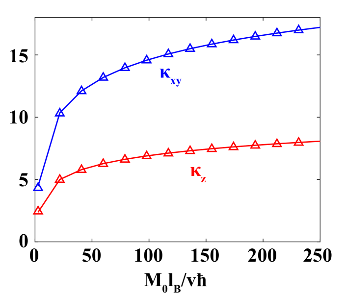
Figure 7: The dielectric constants calculated from definition equations ( Eq. (30) and (31) ) and simplified equations ( Eq. (32) and (33) ) are plotted by triangles and lines, respectively. It shows that the simplified equations give a very good approximation.

In this section, we intend to get a more explicit expression of the dielectric function in the long wavelength limit. Expand $\Lambda_{k_{z}^{\prime}a\alpha\beta}^{*}\left(\mathbf{q}\right)\chi_{k_{z}^{\prime}a\alpha\beta}^{0>}\left(q_{z}\right)\Lambda_{k_{z}^{\prime}a\alpha\beta}\left(\mathbf{q}\right)$ to second order of $\mathbf{q}$, we have

$$\sum_{\alpha\beta}\Lambda_{k_{z}^{\prime}a\alpha\beta}^{*}\left(\mathbf{q}\right)\chi_{k_{z}^{\prime}a\alpha\beta}^{0>}\left(q_{z}\right)\Lambda_{k_{z}^{\prime}a\alpha\beta}\left(\mathbf{q}\right)$$

$$\approx \sum_{\alpha}\chi_{k_{z}^{\prime}a\alpha,-\alpha}^{0>}\left(q_{z}\right)\left[\frac{1}{4}\left(\frac{\partial\theta_{\alpha}}{\partial k_{z}}q_{z}\right)^{2}+\frac{l_{B}^{2}\left(q_{x}^{2}+q_{y}^{2}\right)\sin^{2}\theta_{\alpha}}{16\left|\alpha\right|}\right]$$ (28)

Substitute the definition of the auxiliary angle $\theta_{\alpha}$ in, we get

$$\kappa\left(\mathbf{q}\right) \approx\kappa_{0}+\kappa_{z}\cos^{2}\left\langle\mathbf{q},\mathbf{B}\right\rangle+\kappa_{xy}\sin^{2}\left\langle\mathbf{q},\mathbf{B}\right\rangle$$ (29)

where

$$\kappa_{z}=\frac{e{}^{2}}{8\pi^{2}\epsilon_{0}l_{B}^{2}}\sum_{\alpha=1}^{\infty}\int\frac{2v^{2}\hbar^{2}l_{B}^{-2}\alpha\left(\frac{\partial M\left(k_{z}\right)}{\partial k_{z}}\right)^{2}dk_{z}^{\prime}}{\left(M^{2}\left(k_{z}\right)+2v^{2}\hbar^{2}l_{B}^{-2}\alpha\right)^{\frac{5}{2}}}$$ (30)

$$\kappa_{xy}=\frac{e{}^{2}}{8\pi^{2}\epsilon_{0}l_{B}^{2}}\sum_{\alpha=1}^{\infty}\int\frac{2v^{2}\hbar^{2}dk_{z}^{\prime}}{4\left(M^{2}\left(k_{z}\right)+2v^{2}\hbar^{2}l_{B}^{-2}\alpha\right)^{\frac{3}{2}}}$$ (31)

and $\left\langle\mathbf{q},\mathbf{B}\right\rangle$ is the angle between $\mathbf{q}$ and the magnetic field. Eq. (30)-(31) may be simplified further. Firstly, as the main contribution in the $k_{z}^{\prime}$ integral comes from small $M\left(k_{z}\right)$, we can expand $M\left(k_{z}\right)$ to linear order of $k_{z}$ around each DP. Secondly, the limit $v\hbar l_{B}^{-1}\ll M_{0}$ is assumed such that the Landau level splitting is significantly smaller than the bandwidth and so the summation over $\alpha$ can be approximated by integral. Therefore, we achieve the following formula

$$\kappa_{z}\approx\frac{e{}^{2}u}{3\pi^{2}\epsilon_{0}v^{2}\hbar}\left(0.9+\ln\left(\frac{M_{0}l_{B}}{v\hbar}\right)\right)$$ (32)

$$\kappa_{xy}\approx\frac{e{}^{2}}{4\pi^{2}\epsilon_{0}u\hbar}\left(0.6+\ln\left(\frac{M_{0}l_{B}}{v\hbar}\right)\right)$$ (33)

where $u=\frac{1}{\hbar}M_{0}a_{0}\left|\sin\left(a_{0}k_{c}\right)\right|$ is the Dirac velocity along $z$ direction, and the coefficients $0.9$ and $0.6$ are got by fitting Eq. (32)-(33) with Eq. (30)-(31) numerically. Indeed, Eq. (32)-(33) give very good approximations for Eq. (30)-(31) in a quite wide range. In Fig. (7), we compare the two equations with the parameters used in the paper.

In the end, if we neglect the dependence of $\kappa$ on the direction of $\bf q$, a dielectric constant can be got by an average on the solid angle:

$$\kappa\approx\kappa_{0}+\frac{1}{3}\kappa_{z}+\frac{2}{3}\kappa_{xy}$$ (34)

References

- Klitzing et al. (1980) K. Klitzing, G. Dorda, and M. Pepper, Physical Review Letters 45, 494 (1980).
- Tsui et al. (1982) D. C. Tsui, H. L. Stormer, and A. C. Gossard, Physical Review Letters 48, 1559 (1982).
- Lilly et al. (1999) M. P. Lilly, K. B. Cooper, J. P. Eisenstein, L. N. Pfeiffer, and K. W. West, Phys. Rev. Lett. 83, 824 (1999).
- Du1 (1999) Solid State Communications 109, 389 (1999).
- Feldman et al. (2016) B. E. Feldman, M. T. Randeria, A. Gyenis, F. Wu, H. Ji, R. J. Cava, A. H. MacDonald, and A. Yazdani, Science 354, 316 (2016).
- Celli and Mermin (1965) V. Celli and N. D. Mermin, Physical Review 140, A839 (1965).
- Iye et al. (1984) Y. Iye, L. E. McNeil, and G. Dresselhaus, Phys. Rev. B 30, 7009 (1984).
- Alicea and Balents (2009) J. Alicea and L. Balents, Physical Review B 79, 241101 (2009).
- noa (1987) Japanese Journal of Applied Physics 26, 1913 (1987).
- Tesanovi? and Halperin (1987) Z. Tesanovi? and B. I. Halperin, Physical Review B 36, 4888 (1987).
- Behnia et al. (2007) K. Behnia, L. Balicas, and Y. Kopelevich, Science 317, 1729 (2007).
- Li et al. (2008) L. Li, J. G. Checkelsky, Y. S. Hor, C. Uher, A. F. Hebard, R. J. Cava, and N. P. Ong, Science 321, 547 (2008).
- Nielsen and Ninomiya (1983) H. B. Nielsen and M. Ninomiya, Physics Letters B 130, 389 (1983).
- Son and Spivak (2013) D. T. Son and B. Z. Spivak, Physical Review B 88, 104412 (2013).
- Burkov (2014) A. A. Burkov, Physical Review Letters 113, 247203 (2014).
- Parameswaran et al. (2014) S. Parameswaran, T. Grover, D. Abanin, D. Pesin, and A. Vishwanath, Physical Review X 4, 031035 (2014).
- Xiong et al. (2015) J. Xiong, S. K. Kushwaha, T. Liang, J. W. Krizan, M. Hirschberger, W. Wang, R. J. Cava, and N. P. Ong, Science 350, 413 (2015).
- Lu and Shen (2015) H.-Z. Lu and S.-Q. Shen, Physical Review B 92, 035203 (2015).
- Song et al. (2016) Z. Song, J. Zhao, Z. Fang, and X. Dai, Phys. Rev. B 94, 214306 (2016).
- Rinkel et al. (2016) P. Rinkel, P. L. Lopes, and I. Garate, arXiv preprint arXiv:1610.03073 (2016).
- Zhang et al. (2015) C.-L. Zhang, S.-Y. Xu, C. M. Wang, Z. Lin, Z. Z. Du, C. Guo, C.-C. Lee, H. Lu, Y. Feng, S.-M. Huang, G. Chang, C.-H. Hsu, H. Liu, H. Lin, L. Li, C. Zhang, J. Zhang, X.-C. Xie, T. Neupert, M. Z. Hasan, H.-Z. Lu, J. Wang, and S. Jia, arXiv:1507.06301 [cond-mat] (2015), arXiv: 1507.06301.
- Young et al. (2012) S. M. Young, S. Zaheer, J. C. Y. Teo, C. L. Kane, E. J. Mele, and A. M. Rappe, Physical Review Letters 108, 140405 (2012).
- Wang et al. (2012) Z. Wang, Y. Sun, X.-Q. Chen, C. Franchini, G. Xu, H. Weng, X. Dai, and Z. Fang, Physical Review B 85, 195320 (2012).
- Yang and Nagaosa (2014) B.-J. Yang and N. Nagaosa, Nature Communications 5, 4898 (2014).
- Burkov and Balents (2011) A. Burkov and L. Balents, Physical Review Letters 107, 127205 (2011).
- Wan et al. (2011) X. Wan, A. Turner, A. Vishwanath, and S. Savrasov, Physical Review B 83, 205101 (2011).
- Weng et al. (2015) H. Weng, C. Fang, Z. Fang, B. A. Bernevig, and X. Dai, Physical Review X 5, 011029 (2015).
- Huang et al. (2015) S.-M. Huang, S.-Y. Xu, I. Belopolski, C.-C. Lee, G. Chang, B. Wang, N. Alidoust, G. Bian, M. Neupane, C. Zhang, S. Jia, A. Bansil, H. Lin, and M. Z. Hasan, Nature Communications 6 (2015), 10.1038/ncomms8373.
- Lv et al. (2015) B. Q. Lv, N. Xu, H. M. Weng, J. Z. Ma, P. Richard, X. C. Huang, L. X. Zhao, G. F. Chen, C. E. Matt, F. Bisti, V. N. Strocov, J. Mesot, Z. Fang, X. Dai, T. Qian, M. Shi, and H. Ding, Nature Physics advance online publication (2015), 10.1038/nphys3426.
- Xu et al. (2015a) S.-Y. Xu, I. Belopolski, N. Alidoust, M. Neupane, G. Bian, C. Zhang, R. Sankar, G. Chang, Z. Yuan, C.-C. Lee, S.-M. Huang, H. Zheng, J. Ma, D. S. Sanchez, B. Wang, A. Bansil, F. Chou, P. P. Shibayev, H. Lin, S. Jia, and M. Z. Hasan, Science , aaa9297 (2015a).
- Nie et al. (2017) S. Nie, G. Xu, F. B. Prinz, and S.-C. Zhang, arXiv:1704.02626 [cond-mat] (2017).
- Miransky and Shovkovy (2015) V. A. Miransky and I. A. Shovkovy, Physics Reports 576, 1 (2015).
- Shovkovy (2013) I. A. Shovkovy, in Strongly Interacting Matter in Magnetic Fields (Springer, 2013) pp. 13–49.
- Roy and Sau (2015) B. Roy and J. D. Sau, Phys. Rev. B 92, 125141 (2015).
- Zhang and Shindou (2017) X.-T. Zhang and R. Shindou, Phys. Rev. B 95, 205108 (2017).
- Soluyanov et al. (2015) A. A. Soluyanov, D. Gresch, Z. Wang, Q. Wu, M. Troyer, X. Dai, and B. A. Bernevig, Nature 527, 495 (2015).
- Xu et al. (2015b) Y. Xu, F. Zhang, and C. Zhang, Phys. Rev. Lett. 115, 265304 (2015b).
- (38) To be published.
- Hedin (1965) L. Hedin, Physical Review 139, A796 (1965).
- (40) See the supplemental material at …
- Lerner and Lozovik (1980) I. V. Lerner and Y. E. Lozovik, Journal of Low Temperature Physics 38, 333 (1980).
- Lee and Rice (1979) P. A. Lee and T. M. Rice, Phys. Rev. B 19, 3970 (1979).
- Devereaux and Hackl (2007) T. P. Devereaux and R. Hackl, Reviews of Modern Physics 79, 175 (2007).
- Abrikosov (1998) A. A. Abrikosov, Physical Review B 58, 2788 (1998).
- MacDonald (1994) A. H. MacDonald, arXiv:cond-mat/9410047 (1994), arXiv: cond-mat/9410047.
- Cahill and Glauber (1969) K. E. Cahill and R. J. Glauber, Physical Review 177, 1857 (1969).