Rotating Rayleigh-Taylor turbulence

Abstract

The turbulent Rayleigh–Taylor system in a rotating reference frame is investigated by direct numerical simulations within the Oberbeck-Boussinesq approximation. On the basis of theoretical arguments, supported by our simulations, we show that the Rossby number decreases in time, and therefore the Coriolis force becomes more important as the system evolves and produces many effects on Rayleigh–Taylor turbulence. We find that rotation reduces the intensity of turbulent velocity fluctuations and therefore the growth rate of the temperature mixing layer. Moreover, in presence of rotation the conversion of potential energy into turbulent kinetic energy is found to be less effective and the efficiency of the heat transfer is reduced. Finally, during the evolution of the mixing layer we observe the development of a cyclone-anticyclone asymmetry.

I Introduction

In natural fluid systems, the interface between regions of different density is subject to the well-known Rayleigh-Taylor (RT) instability when the heavier fluid is pushed against the lighter one (see, e.g., Chandrasekhar (1961); Sharp (1984); Abarzhi (2010) for reviews on the subject). In the late stage, this instability evolves in a fully-developed turbulent flow Sharp (1984); Abarzhi (2010); Boffetta and Mazzino (2017). Because of the fact that unstably stratified interfaces are ubiquitous in nature, fluid mixing induced by RT instability and turbulence characterizes many systems, over a huge interval of spatial and temporal scales. Among the possible examples, we mention astrophysical systems, in relation to flame acceleration in type Ia supernova Hillebrandt and Niemeyer (2000); Bell et al. (2004); geological systems, where RT instability has been invoked to explain the initiation and evolution of polydiapirs (domes-in-domes) Weinberg and Schmeling (1992); atmospheric physics, where RT instability has been invoked as a possible explanation for the formation of the mammatus clouds Agee (1975).

Several experimental Read (1984); Dalziel (1993); Dimonte and Schneider (1996); Banerjee and Andrews (2006); Andrews and Dalziel (2010); Banerjee et al. (2010) and numerical Young et al. (2001); Dimonte et al. (2004); Cabot and Cook (2006); Vladimirova and Chertkov (2009); Matsumoto (2009); Biferale et al. (2010) works have investigated the evolution of RT instability and turbulence in different physical conditions. In the limit of small density variations, the simplest mathematical description is provided by the Oberbeck-Boussinesq approximation of two incompressible, miscible fluids. Under these conditions, the seminal paper Chertkov (2003) has shown that three-dimensional RT turbulence can be described as a time-dependent hydrodynamical turbulent flow with a gravity-induced forcing mechanism.

The RT instability and mixing can be significantly affected by the presence of other physical mechanisms, beside gravity, acting on the flow, including compressibility Mitchner and Landshoff (1964); Scagliarini et al. (2010), viscoelasticity Boffetta et al. (2010a), surface tension Chertkov et al. (2005) and physical confinement Lawrie and Dalziel (2011); Boffetta et al. (2012a). An important instance is the case in which the flow is embedded in a rotating reference frame, which causes the emergence of the Coriolis force in the ruling equations. Previous works have shown that the Coriolis force has a stabilizing effect on the RT instability, both in the linear stage Chandrasekhar (1961) and in the weakly nonlinear stage of the perturbation evolution Tao et al. (2013); Carnevale et al. (2002); Baldwin et al. (2015).

In this study we focus on the effects of rotation on the fully developed RT turbulence. We discuss theoretical arguments based on dimensional scaling analysis which predict that the Rossby number decreases in time during the growth of the mixing layer. The Coriolis force is therefore expected to become dominant as the system evolves. This prediction is confirmed by our numerical simulations, which reveals that the turbulent RT system is strongly affected by rotation. In particular, we find that rotation reduces the efficiency of the heat transfer as well as the conversion of potential energy into turbulent kinetic energy. This causes a reduction of the intensity of turbulent velocity fluctuations and slows down the growth of the mixing layer. Interestingly, rotation allows the velocity fluctuations to extend outside the temperature mixing layer. We also observe the development of a cyclone-anticyclone asymmetry which is weakly dependent on the evolution of the mixing layer.

The paper is organized as follow. In Sec. II we introduce the rotating RT system under the Oberbeck-Boussinesq framework and we present mean field (scaling) arguments through which the role of rotation can be inferred. Numerical results from high-resolution DNS of the rotating RT system are presented and discussed in Sec. III concerning the effects of rotation on i) the mixing-layer growth, ii) the heat transfer, iii) the energy spectra, and, finally, iv) the symmetry breaking between cyclones and anticyclones. Final discussions and perspectives are drawn in Sec. IV

II Equation of motion and theoretical considerations

We consider miscible Rayleigh-Taylor turbulence generated at the interface of two layers of fluid with small temperature (density) difference. The initial (at $t=0$) interface is the plane $z=0$, perpendicular to gravity ${\bm{g}}=(0,0,-g)$ and to the uniform rotation ${\bm{\Omega}}=(0,0,\Omega)$. The dynamics is ruled by the Boussinesq equations for an incompressible (${\bm{u}}({\bm{x}},0)=0$) velocity field ${\bm{u}}({\bm{x}},t)=(u,v,w)$ coupled with a temperature field $T({\bm{x}},t)$

$${\partial{\bm{u}}\over\partial t}+{\bm{u}}\cdot{\bm{\nabla}}{\bm{u}}+2{\bm{\Omega}}\times{\bm{u}}=-{\bm{\nabla}}p+\nu\nabla^{2}{\bm{u}}-\beta{\bm{g}}T$$ (1)

$${\partial T\over\partial t}+{\bm{u}}\cdot{\bm{\nabla}}T=\kappa\nabla^{2}T$$ (2)

The reference temperature is set to $T=0$, $\nu$ and $\kappa$ are the kinematic viscosity and diffusivity respectively and $\beta$ is the thermal expansion coefficient. The initial conditions are ${\bm{u}}({\bm{x}},0)=0$, $T({\bm{x}},0)=-(\theta_{0}/2)sgn(z)$ where $\theta_{0}$ is the temperature jump at the interface at $z=0$, which fixes the Atwood number $A=\beta\theta_{0}/2$.

As turbulence develops from the instability at the interface, turbulent kinetic energy in the mixing layer $E=(1/2)\langle|{\bm{u}}|^{2}\rangle$ is produced at the expense of potential energy $P=-\beta g\langle zT\rangle$ (brackets represent integral over the physical domain of volume $L_{x}\times L_{y}\times L_{z}$). The energy balance is written from (1-2) as

$$-{dP\over dt}=\beta g\langle wT\rangle={dE\over dt}+\varepsilon_{\nu}+\beta g{\kappa\theta_{0}\over 2L_{z}}$$ (3)

where $\varepsilon_{\nu}=\nu\langle({\bm{\nabla}}{\bm{u}})^{2}\rangle$ is the viscous energy dissipation and the last term is negligible in the limit of small diffusivity. We define the efficiency $\Sigma$ of turbulent generation as the ratio of the kinetic energy production over potential energy consumption, $\Sigma=-{dE/dt\over dP/dt}$. We anticipate that, although the Coriolis force $2{\bm{\Omega}}\times{\bm{u}}$ does not enter directly in the energy balance (3) it does affect the efficiency of the process which, for $\Omega>0$ is reduced with respect to the value $\Sigma=0.5$ observed for $\Omega=0$ Boffetta et al. (2010b).

The development of the RT instability produces a mixing zone of width $h(t)$ which grows in time. Dimensional arguments derived in absence of rotation Boffetta and Mazzino (2017) predicts that in the turbulent regime the mixing layer grows as $h(t)\simeq Agt^{2}$ and the typical velocity fluctuations inside the mixing layer grow as $u\simeq Agt$ (here $u$ indicates an arbitrary component of the velocity).

Assuming that the dimensional scalings hold also in the rotating case, one obtains the prediction that the dimensionless Rossby number $Ro=w_{rms}/(2\Omega h)$, which measures the relative strength of the inertial forces to the Coriolis forces, should decrease in time as $Ro\simeq 1/(\Omega t)$. In particular, in the case of a weak rotation rate $\Omega$ even if the effect of rotation is negligible at the initial times (ensuring the validity of the dimensional scalings), it becomes more important and eventually competes with the inertial and buoyancy forces for $t\gtrsim 1/\Omega$. For large $\Omega$, this time can be sufficiently small for the rotation to affect already the linear (or quasi-linear) phase of the instability Carnevale et al. (2002); Baldwin et al. (2015).

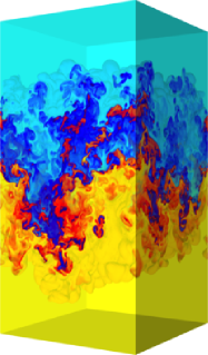
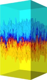
Figure 1: Snapshots of the temperature field at time $t=5.2\tau$ for two simulations with $\Omega\tau=0$ (left) and $\Omega\tau=10$ (right) starting from the same initial conditions. Yellow (blue) represents hot (cold), light (heavy) fluid.

We performed direct numerical simulations (DNS) of the system of equations (1-2) in a periodic domain of size $L_{x}\times L_{y}\times L_{z}$ with $L_{y}=L_{x}$ and $L_{z}=4L_{x}$ by means of a fully parallel pseudo-spectral code at resolution $512\times 512\times 2048$ at different values of rotation $\Omega$. Time evolution is ruled by a second-order Runge-Kutta scheme with explicit integration of the linear terms. For all runs we have $Ag=0.25$, $\theta_{0}=1$ and $Pr=\nu/\kappa=1$. Viscosity is sufficiently large to resolve small scales ($k_{max}\eta\geq 1.3$ at the end of the simulations) and the results are made dimensionless with the box size $L_{x}$, the characteristic time $\tau=(L_{x}/Ag)^{1/2}$ and the characteristic velocity $U=L_{x}/\tau$.

Rayleigh-Taylor instability is seeded by adding to the initial density field a $10\%$ of white noise in a thin layer around the unstable interface at $z=0$. The same realization of the random perturbation is used for all the simulations at different rotation. The simulation is stopped before the mixing layer reaches the dimension of the vertical scale $L_{z}$. We remark that the average quantities in (3) are defined by the integral over the space and therefore their time dependence has an additional $t^{2}$ factor due to the growth of the support of the integral given by the mixing layer width $h(t)$.

Figure 1 shows two snapshots of the temperature field for two simulations at $\Omega\tau=0$ and $\Omega\tau=10$. Rotation produces clear qualitative effects on the temperature field: Thermal plumes are more coherent and elongated in the vertical direction while their vertical velocity is reduced.

III Numerical results

One effect of rotation is to reduce the growth of the mixing layer, a feature which is evident at a qualitative level from Fig. 1. More quantitatively, this reduction is due to a suppression of the vertical velocity fluctuations, measured by $w_{rms}$ and shown in Fig. 2. After the instability, for $t>\tau$, vertical velocity fluctuations in the non-rotating case $\Omega=0$ are observed to grow linearly in time, in agreement with the dimensional prediction $w_{rms}\simeq Agt$. By increasing the rotation velocity, the growth of $w_{rms}$ is strongly depleted and for $\Omega\tau=12.5$ vertical velocities almost saturates at a constant value. The inset of Fig. 2 shows the ratio $w_{rms}/u_{rms}$ of the vertical to the horizontal velocity fluctuations which is found to be weakly dependent on $\Omega$. Therefore also horizontal velocities are reduced and the degree of large-scale anisotropy in the velocity field is not strongly affected by rotation.

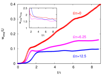
Figure 2: Vertical velocity fluctuations $w_{rms}$ in the mixing layer as a as a function of time for three different rotations, $\Omega\tau=0$ (red squares), $\Omega\tau=6.25$ (pink circles) and $\Omega\tau=12.5$ (blue triangles). Inset: ratio of vertical to horizontal velocity fluctuations as a function of time, for the same values of rotation.

One consequence of the reduction of velocity fluctuations is the slowing down of the growth of the mixing layer in presence of rotation. Different definitions of the mixing layer width $h$ have been proposed, based on either threshold values or integral quantities Dalziel et al. (1999). In the inset of Fig. 3 we plot the time evolution of $h$ defined in terms of the threshold value $z=h/2$ at which the temperature profile $\overline{T}(z)$ reaches a fraction $r$ of the maximum value, i.e. $\overline{T}(\pm h/2)=\mp r\theta_{0}$ Dalziel et al. (1999); Boffetta et al. (2010c) (the overline indicates average over the horizontal planes $L_{x}\times L_{y}$). We observe that rotation indeed induces a strong suppression of the growth of $h(t)$.

A remarkable result shown in Fig. 3 is that the ratio $w_{rms}/h$ is almost independent on $\Omega$ in the late turbulent phase. The natural interpretation is that, since the mixing layer is produced by the velocity fluctuations, $h$ is essentially given by the integral in time of $w_{rms}$ and their ratio becomes $\Omega$-independent.

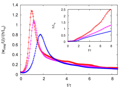
Figure 3: Ratio of the vertical velocity fluctuations $w_{rms}$ to the width of the mixing layer $h$ as a as a function of time for three different rotations, $\Omega\tau=0$ (red squares), $\Omega\tau=6.25$ (pink circles) and $\Omega\tau=12.5$ (blue triangles). Inset: time evolution of the mixing layer width $h$ defined in terms of a threshold $r\theta_{0}$ in the temperature profile, with $r=0.9$.

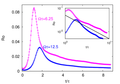
Figure 4: Rossby number $Ro=w_{rms}/(2\Omega h)$ as a function of time for the two rotations $\Omega\tau=6.25$ (pink circles) and $\Omega\tau=12.5$ (blue triangles). Inset: the same quantities in log-log plot. The black line represents $t^{-1}$ scaling.

In Figure  4 we plot the temporal evolution of the Rossby number defined as $Ro=w_{rms}/(2\Omega h)$. Even though in the strongly rotating case the $w_{rms}$ and $h$ might deviate from the scaling expected for $\Omega=0$, we find that the Rossby number, which is proportional to their ratio, decreases with time close to the dimensional prediction $Ro\simeq 1/(\Omega t)$.

Since vertical velocity fluctuations are responsible for the conversion of potential energy into kinetic energy, the potential energy loss $\Delta P(t)=P(0)-P(t)$ is reduced for $\Omega>0$, as shown in Fig. 5. We find that also the efficiency of the process is reduced by rotation: For $\Omega=0$ we have $\Sigma\simeq 0.5$, i.e. about one half of potential energy is converted into large-scale kinetic energy while the other half feeds the turbulent cascade and is eventually dissipated by viscosity Boffetta et al. (2010b). For $\Omega>0$ the efficiency is reduced and we find $\Sigma\simeq 0.3$ for the case $\Omega\tau=12.5$, as shown in Fig. 5, i.e. in this case more potential energy is transferred to small scales and dissipated.

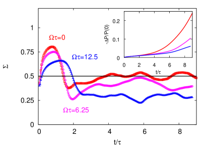
Figure 5: Efficiency of kinetic energy production $\Sigma=-(dE/dt)/(dP/dt)$ as a function of time for three different rotations, $\Omega\tau=0$ (red squares), $\Omega\tau=6.25$ (pink circles) and $\Omega\tau=12.5$ (blue triangles). Inset: potential energy loss $-\Delta P(t)=P(0)-P(t)$ for the same three values of rotations (from top to bottom).

III.1 Integral lengths

Rotation produces different effects on the temperature and on the velocity fields in RT convection. To investigate this issue, we introduce a set of integral lengths based on the vertical profile $f^{(u,w,T)}(z)$ of velocity or temperature variance, defined as $f^{(u)}(z)=\overline{u^{2}}(z)$, $f^{(w)}(z)=\overline{w^{2}}(z)$, $f^{(T)}(z)=\overline{T^{2}}(z)-\overline{T}(z)^{2}$:

$$L^{(u,w,T)}=\left[\frac{\int f^{(u,w,T)}(z)z^{2}dz}{\int f^{(u,w,T)}(z)dz}\right]^{1/2}$$ (4)

where the integral are defined over the whole domain $[0,L_{z}]$. The advantage of this definition with respect to the usual $h(t)$, is that it provides information on the extension of the mixing layer both in terms of (horizontal/vertical) velocity and temperature fluctuations.

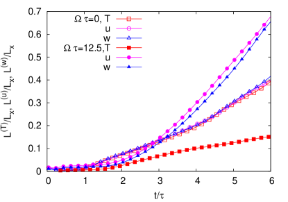
Figure 6: Integral lengths based on the standard deviation of the fluctuation profile of temperature $L^{(T)}$ (red squares), horizontal velocity $L^{(u)}$ (pink circles) and vertical velocity $L^{(w)}$ (blue triangles) without rotation (empty symbols) and for $\Omega\tau=12.5$ (filled symbols).

The evolution of $L^{(u,w,T)}$ is shown in Fig. 6 for two values of $\Omega$. In the absence of rotation the three integral lengths are approximately the same, indicating that temperature and velocity fluctuations are tightly associated within the mixing layer. On the contrary, for $\Omega\tau=12.5$ we observe that while $L^{(T)}$ is reduced (which is already clear from Fig. 1), both $L^{(u)}$ and $L^{(w)}$ increase, approximately by the same amount. This is a manifestation of the Taylor-Proudman phenomenon of bidimensionalization of the velocity field in presence of rotation Tritton (1988) which, becoming almost independent on $z$, extends outside the mixing layer region defined by temperature fluctuations.

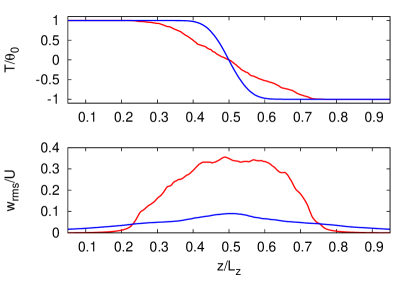
Figure 7: Vertical profiles of mean temperature $\overline{T}(z)$ (upper plot) and of vertical velocity $\overline{w}_{rms}(z)=\overline{w^{2}}(z)^{1/2}$ for the simulation with $\Omega\tau=0$ (red lines) and $\Omega\tau=12.5$ (blue lines) at time $t=6\tau$.

To investigate more in details this issue, in Fig. 7 we plot the temperature profile $\overline{T}$ and the vertical velocity profile $\overline{w}_{rms}=\overline{w^{2}}^{1/2}$ at a late time. It is evident that while in the case $\Omega=0$ the two profiles extend over comparable regions, for the case $\Omega\tau=12.5$ the vertical extension of temperature fluctuations is reduced and at the same time the vertical extension of velocity fluctuations is increased. Summarizing, our findings show that in presence of rotation there is not a unique scale characterizing the mixing layer as velocity and temperature fluctuations define different vertical scales.

III.2 Heat transfer

The efficiency of the transfer of heat in turbulent convection is quantified by the Nusselt number $Nu\equiv\langle wT\rangle h/(\kappa\theta_{0})$ (ratio of the convective to conductive heat transfer) while turbulence intensity is provided by the Reynolds number $Re\equiv|{\bm{u}}|_{rms}h/\nu$. These numbers depends on the dimensionless temperature difference quantified by the Rayleigh number $Ra\equiv\beta g\theta_{0}h^{3}/(\nu\kappa)$. High resolution direct numerical simulations have shown that in Rayleigh-Taylor turbulence $Nu$ and $Re$ displays the so-called ultimate state regime according to which $Nu\simeq Ra^{1/2}Pr^{1/2}$ and $Re\simeq Ra^{1/2}Pr^{-1/2}$ Celani et al. (2006); Boffetta et al. (2009, 2012b) both in two and three dimensions.

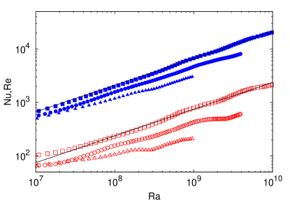
Figure 8: Reynolds number (filled blue symbols) and Nusselt number (open red symbols) as a function of Rayleigh number for the simulations with $\Omega\tau=0$ (squares), $\Omega\tau=6.25$ (circles) and $\Omega\tau=12.5$ (triangles). The black lines represent the ultimate state behavior $Ra^{1/2}$.

We find that rotation reduces the value of $Nu$ both as a function of time (mainly as a consequence of the reduction of $h(t)$) and as a function of $Ra$, i.e. at fixed $h$ as shown in Fig. 8. This latter result means that also the correlation between $w$ and $T$ is reduced by rotation. We find that also $Re$ at given $Ra$ decreases in presence of rotation, mainly as a consequence of the suppression of the velocity fluctuations. Moreover we find that, at larger values of $\Omega$, the ultimate state scaling is violated as both $Nu$ and $Re$ show a dependence on $Ra$ slower than $Ra^{1/2}$.

We remark that our results on the suppression of the heat transport in rotating RT turbulence are qualitatively different to what observed in rotating boundary-forced convective flow, e.g. in Rayleigh-Benard (RB) convection. In the case of rotating RB convection both experiments Liu and Ecke (1997); Zhong et al. (2009); Weiss et al. (2016) and numerical simulations Kunnen et al. (2006); Oresta et al. (2007); Stevens et al. (2013) have shown an enhancement of $Nu$ for moderate values of rotation $\Omega$ with respect to the case $\Omega=0$. This enhancement is ascribed to Ekman pumping which extracts hot and cold fluid from the boundary layers and contributes to the heat flux Kunnen et al. (2006). At large values of rotations (and for large $Ra$) this mechanisms is less efficient and a reduction of $Nu$ is observed. Because of the absence of boundary layers in RT convection, it is not contradictory that here we do not observe an increase of $Nu$ for any value of $\Omega$ and $Ra$.

Beside the differences between RT and RB turbulence due to the boundary conditions, other phenomena occurring in the bulk of rotating convection display interesting similarities between the two systems. In particular, studies of rotating RB has found an increase of the internal mean gradient with decreasing $Ro$ Julien et al. (1996); Hart and Ohlsen (1999); Liu and Ecke (2011) and a corresponding decrease in horizontal versus vertical fluctuations of temperature, which indicates that rotation favors the horizontal transport and suppresses the vertical mixing.

III.3 Energy spectra

In order to investigate the degree of anisotropy at different scales, we computed at given times during the evolution of the system the energy spectra of the horizontal and vertical components of the velocity, indicated respectively as $E_{x}(k)$ and $E_{z}(k)$. The spectra has been computed from the Fourier transform of the velocity fields in the whole periodic domain, and are plotted as a function of the wavenumber $k=(k_{x}^{2}+k_{y}^{2}+k_{z}^{2})^{1/2}$.

In Fig. 9 we compare the horizontal and vertical spectra computed at the same time $t=6\tau$ with and without rotation. We see that for $\Omega=0$ the two spectra are almost identical at high-wavenumbers, indicating the recovering of isotropy in the flow at small scales. Boffetta et al. (2010b). The recovery of small-scale isotropy does not occur in presence of rotation. For $\Omega\tau=12.5$ we find that vertical velocity fluctuations dominates over horizontal velocity fluctuations at all scales. These results indicate that the ratio $E_{z}(k)/E_{x}(k)$ is changed by rotation mostly at small scales, while at large scales rotation reduces both the spectra keeping their ratio almost constant. This is consistent with the weak dependence on $\Omega$ of the ratio $w_{rms}/u_{rms}$ shown in Fig. 2. On the other hand, rotation changes significantly the degree of anisotropy of the velocity gradient. Indeed we measure that the ratio $(\partial_{z}w)_{rms}/(\partial_{x}u)_{rms}$ changes from a value close to one for $\Omega=0$ Boffetta et al. (2010b) to about $0.65$ for $\Omega\tau=12.5$.

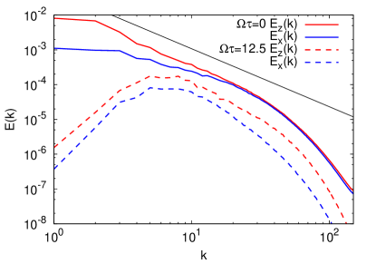
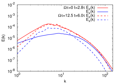
Figure 9: Upper plot: Vertical $E_{z}(k)$ (red) and horizontal $E_{x}(k)$ (blue) kinetic energy spectra computed at the time $t=6.0\tau$ both in the absence of rotation (continuous lines) and with $\Omega\tau=12.5$ (dashed lines). Lower plot: Vertical and horizontal kinetic energy spectra computed at time $t=2.8\tau$ for $\Omega\tau=0$ and at time $t=6.0\tau$ for $\Omega\tau=12.5$ at which the peaks of the vertical spectra are the same.

As rotation slows down the development of turbulence, it is interesting to compare spectra with and without rotation at two different times at which the peaks of the vertical energy spectrum are the same. The comparison of the two spectra is shown in Fig. 9 where we compare the case $\Omega\tau=0$ at $t=2.8\tau$ with the case $\Omega\tau=12.5$ at $t=6.0\tau$. Vertical spectra are almost identical (within statistical fluctuations) while for horizontal spectra the effect of rotation is to reduce small-scale fluctuation in favor of large-scale components.

III.4 Cyclonic-anticyclonic asymmetry

A remarkable feature of turbulent rotating flows is the predominance of cyclones, i.e., vortices co-rotating with the flow, over anticyclones. The cyclone-anticyclone asymmetry has been observed in the atmosphere Hakim and Canavan (2005), and has been studied both in experiments and numerics (for a review see, e.g., Godeferd and Moisy (2015)).

Previous studies Bartello et al. (1994); Deusebio et al. (2014); Gallet et al. (2014); Naso (2015) have investigated the dependence of the asymmetry on the Rossby number and the aspect ratio of the flow. The asymmetry is found to be maximum for $Ro\simeq O(1)$, and vanishes when the flow is confined in a quasi two-dimensional geometry. These results suggest that the mechanisms which produce the asymmetry require the interaction between rotation and turbulent vortex stretching.

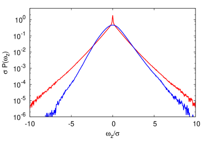
Figure 10: PDF of vertical vorticity computed in the mixing layer of width $h$ at time $t=3.2\tau$ for $\Omega\tau=0$ (red) and $t=5.6\tau$ for $\Omega\tau=12.5$ (blue). At these times the width of the mixing layer in the two cases is the same. The values of the vertical vorticity has been normalized with the standard deviation ($\sigma=0.010$ for $\Omega\tau=0$ and $\sigma=0.039$ for $\Omega\tau=12.5$).

Here we address the question whether or not the cyclonic-anticyclonic asymmetry develops also in the rotating Rayleigh-Taylor turbulence. To address this issue we compute the probability density function (PDFs) of the components of the vorticity field within the mixing layer, where the vorticity is significantly different from zero.

In Figure 10 we compare the PDFs of the vertical component $\omega_{z}$ of the vorticity with and without rotation. The PDFs are computed in the mixing layer of width $h$ at times at which $h$ is the same in the two cases. We find that in the non-rotating case the PDF is symmetric, while in the rotating case it is asymmetric with a positive skewness, which indicates the prevalence of cyclonic vortices, as shown in Fig. 10. A similar result has been observed also for the rotating Rayleigh-Bénard convection Julien et al. (1996).

A quantitative measure of this asymmetry is provided by the skewness of the vertical vorticity:

$$S_{\omega}={\langle\omega_{z}^{3}\rangle\over\langle\omega_{z}^{2}\rangle^{3/2}}$$ (5)

where the average is here computed within the mixing layer.

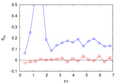
Figure 11: Time evolution of the skewness $S_{\omega}=\langle\omega_{z}^{3}\rangle/\langle\omega_{z}^{2}\rangle^{3/2}$ for $\Omega\tau=0$ (red) and $\Omega\tau=12.5$ (blue).

The time evolution of $S_{\omega}$ is shown in Fig. 11 for two cases with and without rotation. While for $\Omega=0$ we have a skewness consistent with zero, for $\Omega\tau=12.5$ we observe, after the development of the turbulent phase, a value $S_{\omega}\simeq 0.15$ almost independent on time. The weak time-dependence of the skewness is somehow surprising, because the cyclonic-anticyclonic asymmetry is known to depend on the Rossby number Deusebio et al. (2014), which in this case decreases in time as $Ro\simeq 1/\Omega t$. One possible explanation is that is our simulations the time dependence of $Ro$ is too weak (see Fig. 3) to appreciate a significant variation of the asymmetry. We conclude by remarking that the other two components of the vorticity are symmetric also in presence of rotation.

IV Conclusions

In this paper we have studied the effect of rotation along the vertical axis on the development and the mixing properties of Rayleigh-Taylor turbulence in the Boussinesq approximation of incompressible flow. We have found that rotation reduces the intensity of turbulent velocity fluctuations, a generalization of the known stabilizing effect on the linear phase Chandrasekhar (1961); Carnevale et al. (2002). As a consequence, the temporal growth of the mixing layer is observed to be reduced with respect the case without rotation. Rotation also reduces the efficiency of the conversion of the available potential energy into large-scale kinetic energy, and relatively more energy is dissipated at small scales. The analysis of the kinetic energy spectra revealed that rotation induces a strong anisotropy at small scales, where vertical velocity fluctuations dominate over horizontal ones.

In spite of the reduction of the intensity of velocity fluctuations, we found that rotation allows them to extends in a broader region, a manifestation of the Taylor-Proudman theorem on the bidimensionalization of the flow, while the scale associated to temperature fluctuations is reduced. These results imply that in presence of rotation the mixing layer has a complex structure which cannot be characterized by a single scale. The presence of different characteristic scales for velocity and temperature has important dynamical consequences. Indeed, the analysis of our numerical simulations show that the heat transfer, quantified by the Nusselt number, is reduced by rotation not only as a function of time, but also at a given Rayleigh number (i.e. width of the mixing layer). This means that rotation reduces the correlation $\langle wT\rangle$ between the temperature and the vertical velocity.

Finally, we have analyzed the cyclone-anticyclone asymmetry induced by rotation. We have found that, as in other turbulent systems, rotation induces an asymmetry in the PDF of the vertical vorticity which displays a a positive (with respect to the background rotation) skewness. The skewness is found to be approximatively constant during the development of the turbulent mixing layer.

In conclusion, we found that rotation induces a rich and complex phenomenology in Rayleigh-Taylor turbulence. As RT turbulence is a prototypical example of bulk turbulent convection, not driven by boundary layers, we expect similar effects in other convective flows dominated by bulk properties. Further numerical and experimental work in this direction would be extremely interesting.