Towards Automated Network Mitigation Analysis

Towards Automated Network Mitigation Analysis (extended)

Abstract.

Penetration testing is a well-established practical concept for the identification of potentially exploitable security weaknesses and an important component of a security audit. Providing a holistic security assessment for networks consisting of several hundreds hosts is hardly feasible though without some sort of mechanization. Mitigation, prioritizing counter-measures subject to a given budget, currently lacks a solid theoretical understanding and is hence more art than science. In this work, we propose the first approach for conducting comprehensive what-if analyses in order to reason about mitigation in a conceptually well-founded manner. To evaluate and compare mitigation strategies, we use simulated penetration testing, i.e., automated attack-finding, based on a network model to which a subset of a given set of mitigation actions, e.g., changes to the network topology, system updates, configuration changes etc. is applied. Using Stackelberg planning, we determine optimal combinations that minimize the maximal attacker success (similar to a Stackelberg game), and thus provide a well-founded basis for a holistic mitigation strategy. We show that these Stackelberg planning models can largely be derived from network scan, public vulnerability databases and manual inspection with various degrees of automation and detail, and we simulate mitigation analysis on networks of different size and vulnerability.

Notes about this version

The first version of this article was published on arXiv under the title ‘Simulated Penetration Testing and Mitigation Analysis’ (Backes et al., 2017). The mitigation analysis formalism was later dubbed ‘Stackelberg planning’ and discussed in a more general scope in a separate publication (Speicher et al., 2018). The present version thus concentrates on the application to simulated pentesting. In comparison to the previous version, the algorithmic implementation was removed (it can be found (Speicher et al., 2018)), the presentation was streamlined, typos were fixed and the title changed to reflect the new focus.

1. Introduction

Penetration testing (pentesting) evaluates the security of an IT infrastructure by trying to identify and exploit vulnerabilities. It constitutes a central, often mandatory component of a security audit, e.g., the Payment Card Industry Data Security Standard prescribes ‘network vulnerability scans at least quarterly and after any significant change in the network’ (Calder and Williams, 2014). Network pentests are frequently conducted on networks with hundreds of machines. Here, the vulnerability of the network is a combination of host-specific weaknesses that compose to an attack. Consequently, an exhausting search is out of question, as the search space for these combinations grows exponentially with the number of hosts. Choosing the right attack vector requires a vast amount of experience, arguably making network pentesting more art than science.

While it is conceivable that an experienced analyst comes up with several of the most severe attack vectors, this is not sufficient to provide for a sound mitigation strategy, as the evaluation of a mitigation strategy requires a holistic security assessment. So far, there is no rigorous foundation for what is arguably the most important step, the step after the pentest: how to mitigate these vulnerabilities.

In practice, the severity of weaknesses is assessed more or less in isolation, proposed counter-measures all too often focus on single vulnerabilities, and the mitigation path is left to the customer. There are exceptions, but they require considerable manual effort.

Simulated pentesting was proposed to automate large-scale network testing by simulating the attack finding process based on a logical model of the network. The model may be generated from network scans, public vulnerability databases and manual inspection with various degrees of automation and detail. To this end, AI planning methods have been proposed (Boddy et al., 2005; Lucangeli et al., 2010) and in fact used commercially, at a company called Core Security, since at least 2010 (Corporation, [n. d.]). These approaches, which derive from earlier approaches based on attack graphs (Phillips and Swiler, 1998; Schneier, 1999; Sheyner et al., 2002), assume complete knowledge over the network configuration, which is often unavailable to the modeller, as well as the attacker. We follow a more recent approach favouring Markov decisions processes (MDP) as the underlying state model to obtain a good middle ground between accuracy and practicality (Durkota and Lisý, 2014; Hoffmann, 2015) (we discuss this in detail as part of our related work discussion, Section 2).

Simulated pentesting has been used to great success, but an important feature was overseen so far. If a model of the network is given, one can reason about possible mitigations without implementing them – namely, by simulating the attacker on a modified model. This allows for analysing and comparing different mitigation strategies in terms of the (hypothetical) network resulting from their application. This problem was recently introduced as Stackelberg planning in the AI community (Speicher et al., 2018). Algorithmically, the attacker-planning problem now becomes part of a larger what-if planning problem, in which the best mitigation plans are constructed. This min-max notion is similar to a Stackelberg game, which are frequently used in security games (Korzhyk et al., 2011). The foundational assumption is that the defender acts first, while the adversary can choose her best response after observing this choice, similar to a market leader and her followers. The algorithm thus provides a well-founded basis for a holistic mitigation strategy.

Mitigation actions can represent, but are not limited to, changes to the network topology, e.g., adding a packet filter, system updates that remove vulnerabilities, and configuration changes or application-level firewalls which work around issues. While, e.g., an application-level firewall might be an efficient temporary workaround for a vulnerability that affects a single host, contracting a software vendor to provide a patch might be more cost-efficient in case the vulnerability appears throughout the network. To reflect cases like this, mitigation actions are assigned a cost for their first application (set-up cost), and another potentially different cost for all subsequent applications (application cost). The algorithm computes optimal combinations w.r.t.  minimizing the maximal attacker success for a given budget, and proposes dominant mitigation strategies with respect to cost and attacker success probability.

After discussing related work in Section 2 and giving a running example in Section 3, we present the mitigation analysis model in Section 4, framed in a formalism suited for a large range of mitigation/attack planning problems. In Section 5, we show how to derive these models by scanning a given network using the Nessus network-vulnerability scanner. The attacker action model is then derived using a vulnerability database and data associated using the Common Vulnerability Scoring System (CVSS). This methodology provides a largely automated method of deriving a model (only the network topology needs to be given by hand), which can then be used as it is, or further refined. In Section 6, we evaluate our algorithms w.r.t. problems from this class, derived from a vulnerability database and a simple scalable network topology.

2. Related Work

Our work is rooted in a long line of research on network security modeling and analysis, starting with the consideration of attack graphs. The simulated pentesting branch of this research essentially formulates attack graphs in terms of standard sequential decision making models — attack planning — from AI. We give a brief background on the latter first, before considering the history of attack graph models.

Automated Planning is one of the oldest sub-areas of AI (see (Ghallab et al., 2004) for a comprehensive introduction). The area is concerned with general-purpose planning mechanisms that automatically find a plan, when given as input a high-level description of the relevant world properties (the state variables), the initial state, a goal condition, and a set of actions, where each action is described in terms of a precondition and a postcondition over state variable values. In classical planning, the initial state is completely known and the actions are deterministic, so the underlying state model is a directed graph (the state space) and the plan is a path from the initial state to a goal state in that graph. In probabilistic planning, the initial state is completely known but the action outcomes are probabilistic, so the underlying state model is a Markov decision process (MDP) and the plan is an action policy mapping states to actions.In partially observable probabilistic planning, we are in addition given a probability distribution over the possible initial states, so the underlying state model is a partially observable MDP (POMDP).

The founding motivation for Automated Planning mechanisms is flexible decision taking in autonomous systems, yet the generality of the models considered lends itself to applications as diverse as the control of modular printers (Ruml et al., 2011), natural language sentence generation (Koller and Hoffmann, 2010; Koller and Petrick, 2011), greenhouse logistics (Helmert and Lasinger, 2010), and, in particular, network security penetration testing (Boddy et al., 2005; Lucangeli et al., 2010; Sarraute et al., 2012; Durkota and Lisý, 2014; Hoffmann, 2015). This latter branch of research — network attack planning as a tool for automated security testing — has been coined simulated pentesting, and is what we continue here.

Simulated pentesting is rooted in the consideration of attack graphs, first introduced by Philipps and Swiler (Phillips and Swiler, 1998). An attack graph breaks down the space of possible attacks into atomic components, often referred to as attack actions, where each action is described by a conjunctive precondition and postcondition over relevant properties of the system under attack. This is closely related to the syntax of classical planning formalisms. Furthermore, the attack graph is intended as an analysis of threats that arise through the possible combinations of these actions. This is, again, much as in classical planning. That said, attack graphs come in many different variants, and the term “attack graph” is rather overloaded. From our point of view here, relevant lines of distinction are the following.

In several early works (e. g. (Schneier, 1999; Templeton and Levitt, 2000)), the attack graph is the attack-action model itself, presented to the human as an abstracted overview of (atomic) threats. It was then proposed to instead reason about combinations of atomic threats, where the attack graph (also: “full” attack graph) is the state space arising from all possible sequencings of attack actions (e. g. (Ritchey and Ammann, 2000; Sheyner et al., 2002)). Later, positive formulations — positive preconditions and postconditions only — where suggested as a relevant special case, where attackers keep gaining new assets, but never lose any assets during the course of the attack (Templeton and Levitt, 2000; Ammann et al., 2002; Jajodia et al., 2005; Ou et al., 2006; Noel et al., 2009; Ghosh and Ghosh, 2009). This restriction drastically simplifies the computational problem of non-probabilistic attack graph analysis, yet it also limits expressive power, especially in probabilistic models where a stochastic effect of an attack action (e. g., crashing a machine) may be detrimental to the attacker’s objectives.

A close relative of attack graphs are attack trees (e. g. (Schneier, 1999; Mauw and Oostdijk, 2005)). These arose from early attack graph variants, and developed into ‘Graphical Security Models’ (Kordy et al., 2013): Directed acyclic AND/OR graphs organizing known possible attacks into a top-down refinement hierarchy. The human user writes that hierarchy, and the computer analyzes how attack costs and probabilities propagate through the hierarchy. In comparison to attack graphs and planning formulations, this has computational advantages, but cannot find unexpected attacks, arising from unforeseen combinations of atomic actions.

Probabilistic models of attack graphs/trees have been considered widely (e. g. (Buldas et al., 2006; Niitsoo, 2010; Sarraute et al., 2011; Singhal and Ou, 2011; Buldas and Stepanenko, 2012; Lisý and Píbil, 2013; Homer et al., 2013)), yet they weren’t, at first, given a formal semantics in terms of standard sequential decision making formalisms. The latter was done later on by the AI community in the simulated pentesting branch of research. After initial works linking non-probabilistic attack graphs to classical planning (Boddy et al., 2005; Lucangeli et al., 2010), Sarraute et al. (Sarraute et al., 2012) devised a comprehensive model based on POMDPs, designed to capture penetration testing as precisely as possible, explicitly modeling the incomplete knowledge on the attacker’s side, as well as the development of that knowledge during the attack. As POMDPs do not scale — neither in terms of modeling nor in terms of computation — it was thereafter proposed to use MDPs as a more scalable intermediate model (Durkota and Lisý, 2014; Hoffmann, 2015). and were later linked to to classical planning (Boddy et al., 2005; Lucangeli et al., 2010). More precise formulations in terms of partially observable MDPs were proposed for their ability to model incomplete knowledge on the attacker’s side (Sarraute et al., 2012). As POMDPs do not scale — neither in terms of modeling nor in terms of computation — it was thereafter proposed to use MDPs as a more scalable intermediate model (Durkota and Lisý, 2014; Hoffmann, 2015). Here we build upon this latter model.

Stackelberg planning (Speicher et al., 2018) models not only the attacker, but also the defender, and in that sense relates to more general game-theoretic security models. The most prominent application of such models thus far concerns physical infrastructures and defenses (e. g. (Tambe, 2011)), quite different from the network security setting. A line of research considers attack-defense trees (e. g. (Kordy et al., 2010; Kordy et al., 2013)), not based on standard sequential decision making formalisms. Some research considers pentesting but from an abstract theoretical perspective (Böhme and Félegyházi, 2010). A basic difference to most game-theoretic models is that our mitigation analysis does not consider arbitrarily long exchanges of action and counter-action, but only a single such exchange: defender applies network fixes, attacker attacks the fixed network. The latter relates to Stackelberg competitions, yet with interacting state-space search models underlying each side of the game.

3. Running Example

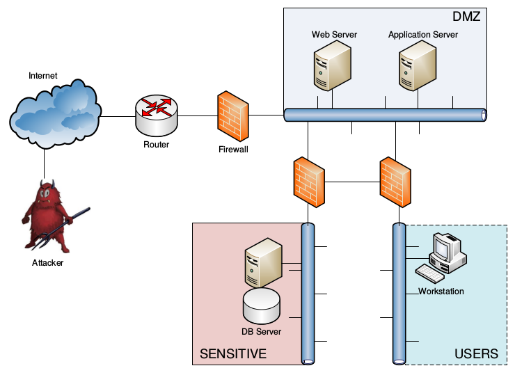
Figure 1. Network structure in our running example. (Figure adapted from Sarraute et al. (Sarraute et al., 2012).)

We will use the following running example for easier introduction of our formalism and to foreshadow the modelling of networks which we will use in Section 5. Let us consider a network of five hosts, i.e., computers that are assigned an address at the network layer. It consists of a webserver $W$, an application server $A$, a database server $D$, and a workstation $S$. We partition the network into three zones called as follows: 1) the sensitive zone, which contains important assets, i.e., the database server $D$ 2) the DMZ, which contains the services that need to be available from the outside, i.e., $A$ and $W$, 3) the user zone, in which $S$ is placed and 4) the internet, which is assumed under adversarial control by default and contains at least a host $I$.

These zones are later (cf. Section 6) used to define the adversarial goals and may consist of several subnets. For now, each zone except the internet consists of exactly one subnet. These subnets are interconnected, with the exception of the internet, which is only connected to the DMZ. Firewalls filter some packets transmitted between the zones. We will assume that the webserver can be accessed via HTTPS (port 443) from the internet.

4. Mitigation analysis as Stackelberg planning

It was recently proposed to model penetration testing and mitigation tasks as Stackelberg planning task (Speicher et al., 2018). We review this formalism and show how vulnerability analysis can be mapped onto it.

Intuitively, the attacks we consider might make a service unavailable, but not physically remove a host from the network or add a physical connection between two hosts. We thus distinguish between network propositions and attacker propositions, where the former describes the network infrastructure and persistent configuration, while the latter describes the attacker’s advance through the network. By means of this distinction, we may assume the state of the network to be fixed, while everything else can be manipulated by the attacker. The network state will, however, be altered during mitigation analysis, which we will discuss in more detail afterwards.

Networks are logically described through a finite set of network propositions $\mathsf{P}^{\mathsf{N}}$. A concrete network state is a subset of network propositions $s^{\mathsf{N}}\subseteq\mathsf{P}^{\mathsf{N}}$ that are true in this state. All propositions $p\not\in s^{\mathsf{N}}$ are considered to be false.

Example 4.1.

In the running example, the network topology is described in terms of network propositions $\mathsf{subnet}(s,h)\in\mathsf{P}^{\mathsf{N}}$ assigning a host $h$ to a subnet $s$, e.g., $\mathsf{subnet}(\mathsf{sensitive},D)\in\mathsf{P}^{\mathsf{N}}$. Connectivity is defined between subnets, e.g., $\mathsf{haclz}(\mathsf{internet},\mathsf{dmz},443,\mathsf{tcp})\in\mathsf{P}^{\mathsf{N}}$ indicates that TCP packets with destination port $443$ (HTTPS) can pass from the internet into the DMZ. We assume that the webserver $W$, the workstation $S$ and the database server $D$ are vulnerable, e.g., $\mathsf{vul\_exists}(\mathit{cve}_{W},W,443,\mathsf{tcp},\mathsf{}in\-te\-gri\-ty)\in\mathsf{P}^{\mathsf{N}}$ for a vulnerability with CVE identifier $\mathit{cve}_{W}$ affecting $W$ on TCP port 443, that compromises integrity.

We formalize network penetration tests in terms of a probabilistic planning problem:

Definition 4.2 (penetration testing task (Speicher et al., 2018)).

A penetration testing task is a tuple $\Pi=(\mathsf{P}^{\mathsf{A}},{\mathsf{A}},\mathsf{I}^{\mathsf{A}},\mathsf{G},b^{\mathsf{A}}_{0})$ consisting of:

• a finite set of attacker propositions $\mathsf{P}^{\mathsf{A}}$,

• a finite set of (probabilistic) attacker actions ${\mathsf{A}}$ (cf. Definition 4.4),

• the attacker’s initial state $\mathsf{I}^{\mathsf{A}}\subseteq\mathsf{P}^{\mathsf{A}}$,

• a conjunction $\mathsf{G}$ over attacker proposition literals, called the attacker goal, and

• a non-negative attacker budget $b^{\mathsf{A}}\in\mathbb{R}^{+}\cup\{\infty\}$, including the special case of an unlimited budget $b^{\mathsf{A}}=\infty$.

The objective in solving such a task — the attacker’s objective — will be to maximize attack probability, i. e., to find action strategies maximizing the likelihood of reaching the goal, which we will specify in more detail. The attacker proposition are used to describe the state of the attack, e. g., dynamic aspects of the network and which hosts the attacker has gained access to.

Example 4.3.

Consider an attacker that initially controls the internet, i.e., $\mathsf{controls}(I)\in\mathsf{I}^{\mathsf{A}}$ and has not yet caused $W$ to crash, $\mathsf{available}(W)\in\mathsf{I}^{\mathsf{A}}$. The attacker’s aim might be to inflict a privacy-loss on $D$, i.e., $\mathsf{compromised}(D,\mathsf{privacy})$, with a budget $b^{\mathsf{A}}$ of $3$ units, which relate to the attacker actions below.

The attacks themselves are described in terms of actions which can depend on both network and attacker propositions, but only influence the attacker state.

Definition 4.4 (attacker actions (Speicher et al., 2018)).

An attacker action $a\in{\mathsf{A}}$ is a tuple $(\mathit{pre}^{\mathsf{N}}(a),\mathit{pre}^{\mathsf{A}}(a),c(a),O(a))$ where

• $\mathit{pre}^{\mathsf{N}}(a)$ is a conjunction over network proposition literals called the network-state precondition,

• $\mathit{pre}^{\mathsf{A}}(a)$ is a conjunction over attacker proposition literals called the attacker-state precondition,

• $c(a)\in\mathbb{R}^{+}$ is the action cost, and

• $O(a)$ is a finite set of outcomes, each $o\in O(a)$ consisting of an outcome probability $p(o)\in(0,1]$ and a postcondition $\mathit{post}(o)$ over attacker proposition literals. We assume that $\sum_{o\in O(a)}p(o)=1$.

The stochastic effect $\mathit{post}(o)\in O(a)$ can be used to model attacks that are probabilistic by nature, as well as to model incomplete knowledge (on the attacker’s side) about the actual network configuration. Because $\mathit{post}(o)$ is limited to attacker propositions, we implicitly assume that the attacker cannot have a direct influence on the network itself. Although this is restrictive, it is a common assumption in the penetration testing literature (e. g. (Jajodia et al., 2005; Ou et al., 2006; Noel et al., 2009; Ghosh and Ghosh, 2009)). The attacker action cost can be used to represent the effort the attacker has to put into executing what is being abstracted by the action. This can, e.g., be the estimated amount of time an action requires to be carried out, or the actual cost in terms of monetary expenses.

Example 4.5.

If an attacker controls a host which can access a second host that runs a vulnerable service, it can compromise the second host w.r.t. privacy, integrity or availability, depending on the vulnerability. This is reflected, e.g., by an attacker action $a\in{\mathsf{A}}$ which requires access to a vulnerable $W$ within the DMZ, via the internet, s.t. $\mathit{pre}^{\mathsf{N}}(a)=\mathsf{subnet}(\mathsf{dmz},W)\land\mathsf{subnet}(\mathsf{internet},I)\land\mathsf{haclz}(\mathsf{internet},\mathsf{dmz},443,\mathsf{tcp})\land\mathsf{vul\_exists}(\mathit{cve}_{W},W,443,\mathsf{tcp},\mathsf{}in\-te\-gri\-ty)$. In addition, $I$ needs to be under adversarial control (which is the case initially), and $W$ be available: $\mathit{pre}^{\mathsf{A}}(a)=\mathsf{controls}(I)\land\mathsf{available}(W)$.

The cost of this known vulnerability may be set to $c(a)=1$, in which case the adversarial budget above relates to the number of such vulnerabilities used. More elaborate models are possible to distinguish known vulnerabilities from zero-day exploits which may exists, but only be bought or developed at high cost, or threats arising from social engineering.

We define three different outcomes $O(a)=\{o_{\mathit{success}},\allowbreak o_{\mathit{fail}},\allowbreak o_{\mathit{crash}}\}$ with probabilities

• $\mathit{post}(o_{\mathit{success}})=\allowbreak\mathsf{compromised}(W,\mathsf{}in\-te\-gri\-ty)\allowbreak\land\mathsf{controls}(W)$ in case the exploit succeeds,

• $\mathit{post}(o_{\mathit{fail}})=\top$ in case the exploit has no effect and

• and $\mathit{post}(o_{\mathit{crash}})=\neg\mathsf{available}(W)$ if it crashes $W$.

For example, we may have $p(o_{\mathit{success}})=0.5$, $p(o_{\mathit{fail}})=0.49$, and $p(o_{\mathit{crash}})=0.01$ because the exploit is of stochastic nature, with a small probability to crash the machine.

Regarding the first action outcome, $o_{\mathit{success}}$, note that we step here from a vulnerability that affects integrity, to the adversary gaining control over $W$. This is, of course, not a requirement of our formalism; it is a practical design decision that we make in our current model acquisition setup (and that was made by previous works on attack graphs with similar model acquisition machinery e. g. (Ou et al., 2006; Singhal and Ou, 2011)), because the vulnerability databases available do not distinguish between a privilege escalation and other forms of integrity violation. We get back to this in Section 5. Regarding the third action outcome, $o_{\mathit{crash}}$, note that negation is used to denote removal of literals, i. e., the following attacker state will not contain $\mathsf{available}(W)$ anymore, so that all vulnerabilities on $W$ cease to be useful to the attacker.

The syntax and state transition semantics just specified is standard probabilistic planning. Thus, the state space of a penetration testing task can be viewed as a Markov decision process (MDP). A solution for an MDP is called policy and there are various objectives for these policies, i. e., notions of optimality, in the literature. For attack planning, arguably the most natural objective is success probability: the likelihood that the attack policy will reach a goal state.

Unfortunately, it is EXPTIME-complete to find such an optimal policy in general (Littman et al., 1998). Furthermore, recent experiments have shown that, even with very specific restrictions on the action model, finding an optimal policy for a penetration testing task is feasible only for small networks of up to 25 hosts (Steinmetz et al., 2016). For the sake of scalability and following the lines of Stackelberg Planning (Speicher et al., 2018), we thus focus on finding critical attack paths, instead of entire policies. In a nutshell, a critical attack path is a sequence of actions whose success probability is maximal. We will also refer to such paths as optimal attack plans, or optimal attack action sequences. In contrast to policies, if any action within a critical attack path does not result in the desired outcome, we consider the attack to have failed. Critical attack paths are conservative approximations of optimal policies, i. e., the success probability of a critical attack path is a lower bound on the success probability of an optimal policy.

Example 4.6.

Reconsider the outcomes of action $a$ from Example 4.5, $O(a)=\{o_{\mathit{success}},o_{\mathit{fail}},o_{\mathit{crash}}\}$. Assuming a reasonable set of attacker actions similar to the previous examples, no critical path will rely on the outcomes $o_{\mathit{fail}}$ or $o_{\mathit{crash}}$, as otherwise $a$ would be redundant or even counter-productive. Thus the distinction between these two kinds of failures becomes unnecessary, which is reflected in the models we generate in Section 5 and 6. The downside of considering only single paths instead of policies can be observed in the following example. Consider the case where a second action $a^{\prime}$ has similar outcomes $O(a^{\prime})=\{o^{\prime}_{\mathit{success}},o^{\prime}_{\mathit{fail}},o^{\prime}_{\mathit{crash}}\}$ to $a$, but $p(o^{\prime}_{\mathit{success}})<p(o_{\mathit{success}})$ while $p(o^{\prime}_{\mathit{crash}})$ is considerably smaller than $p(o_{\mathit{crash}})$. Assuming that $W$ is the only host that can be used to reach $S$ or $D$, an optimal policy might chose $a^{\prime}$ in favour of $a$, while a critical attack path will insist on $a$.

Finding possible attacks, e. g., through a penetration testing task as defined above, is only the first step in securing a network. Once these are identified, the analyst or the operator need to come up with a mitigation plan to mitigate or contain the identified weaknesses. This task can be formalized as follows.

Definition 4.7 (mitigation-analysis task (Speicher et al., 2018)).

Let $\mathsf{P}^{\mathsf{N}}$ be a set of network propositions, and let $\Pi=(\mathsf{P}^{\mathsf{A}},{\mathsf{A}},\mathsf{I}^{\mathsf{A}},\mathsf{G},b^{\mathsf{A}}_{0})$ be a penetration testing task. A $\Pi$ mitigation-analysis task is a triple $\mathsf{M}=(\mathsf{I}^{\mathsf{N}},{\mathsf{F}},b^{\mathsf{M}}_{0})$ consisting of

• the initial network state $\mathsf{I}^{\mathsf{N}}\subseteq\mathsf{P}^{\mathsf{N}}$,

• a finite set of fix-actions ${\mathsf{F}}$, and

• the mitigation budget $b^{\mathsf{M}}_{0}\in\mathbb{R}^{+}\cup\{\infty\}$.

The objective in solving such a task — the defender’s objective —will be to find dominant mitigation strategies within the budget, i. e., fix-action sequences that reduce the attack probability as much as possible while spending the same cost. We now specify this in detail.

Fix-actions encode modifications of the network mitigating attacks simulated through $\Pi$.

Definition 4.8 (fix-actions (Speicher et al., 2018)).

Each fix-action $f\in{\mathsf{F}}$ is a triple $(\mathit{pre}(f),\mathit{post}(f),c^{\mathsf{M}}(f))$ of precondition $\mathit{pre}(f)$ and postcondition $\mathit{post}(f)$, both conjunctions over network proposition literals, and fix-action cost $c^{\mathsf{M}}(f)\in\mathbb{R}^{+}$.

We call $f$ applicable to a network state $s^{\mathsf{N}}$ if $\mathit{pre}(f)$ is satisfied in $s^{\mathsf{N}}$. The set of applicable $f$ in $s^{\mathsf{N}}$ is denoted by $\mathit{app}(s^{\mathsf{N}})$. The result of this application is given by the state $s^{\mathsf{N}}\llbracket f\rrbracket$ which contains all propositions with positive occurrences in $\mathit{post}(f)$, and all propositions of $s^{\mathsf{N}}$ whose negation is not contained in $\mathit{post}(f)$.

Example 4.9.

Removing a vulnerability by, e.g., applying a patch, is modelled as a fix-action $f$ with $\mathit{pre}(f)=\mathsf{vul\_exists}(\mathit{cve}_{W},\allowbreak W,443,\allowbreak\mathsf{tcp},\allowbreak\mathsf{}in\-te\-gri\-ty)$, $\mathit{post}(f)=\neg\mathit{pre}(f)$ and cost $1$.

We can represent adding a firewall between the DMZ and the internet, assuming it was not present before, as a fix-action with $\mathit{pre}(f)=\mathsf{haclz}(\allowbreak\mathsf{internet},\mathsf{dmz},443,\mathsf{tcp})\land\neg\mathsf{fwapplied}(z_{2})$, $\mathit{post}(f)=\neg\mathsf{haclz}(\allowbreak\mathsf{internet},\mathsf{dmz},443,\mathsf{tcp})\land\mathsf{fwapplied}(z_{2})$ and cost $100$. It is much cheaper to add a rule to an existing firewall than to add a firewall, which can be represented by a similar rule with $\mathsf{fwapplied}(z_{2})$ instead of $\neg\mathsf{fwapplied}(z_{2})$ in the precondition, and lower cost.

Note that, in contrast to attacker actions, fix-actions $f$ are deterministic. A sequence of fix-actions can be applied to a network in order to lower the success probability of an attacker.

Definition 4.10 (mitigation strategy (Speicher et al., 2018)).

A sequence of fix-actions $\sigma=f_{1},\dots,f_{n}$ is called a mitigation strategy if it is applicable to the initial network state and its application cost is within the available mitigation budget. , where

• $f_{1},\dots,f_{n}$ are said to be applicable to a network state $s^{\mathsf{N}}$ if $f_{1}$ is applicable to $s^{\mathsf{N}}$ and $f_{2},\dots,f_{n}$ are applicable to $s^{\mathsf{N}}\llbracket f_{1}\rrbracket$. The resulting state is denoted $s^{\mathsf{N}}\llbracket f_{1},\dots,f_{n}\rrbracket$.

• Applying $f_{1},\dots,f_{n}$ costs $c^{\mathsf{M}}(f_{1},\dots,f_{n})=\sum_{i=1}^{n}c^{\mathsf{M}}(f_{i})$.

To evaluate and compare different mitigation strategies, we consider their effect on the optimal attack. As discussed in the previous section, for the sake of scalability we use critical attack paths (optimal i. e. maximum-success-probability attack-action sequences) to gauge this effect, rather than full optimal MDP policies. As attacker actions in $\Pi$ may contain a precondition on the network state, changing the network state affects the attacker actions in the state space of $\Pi$, and consequently the critical attack paths. To measure the impact of a mitigation strategy, we define $p^{*}(s^{\mathsf{N}})$ to be the success probability of a critical attack path in $s^{\mathsf{N}}$, or $p^{*}(s^{\mathsf{N}})=0$ if there is no critical attack path (and thus there is no way in which the attacker can achieve its goal).

Definition 4.11 (dominance, solution (Speicher et al., 2018)).

Let $\sigma_{1},\sigma_{2}$ be two mitigation strategies. $\sigma_{1}$ dominates $\sigma_{2}$ if

1. $p^{*}(\mathsf{I}^{\mathsf{N}}\llbracket\sigma_{1}\rrbracket)<p^{*}(\mathsf{I}^{\mathsf{N}}\llbracket\sigma_{2}\rrbracket)$ and $c^{\mathsf{M}}(\sigma_{1})\leq c^{\mathsf{M}}(\sigma_{2})$, or

2. $p^{*}(\mathsf{I}^{\mathsf{N}}\llbracket\sigma_{1}\rrbracket)\leq p^{*}(\mathsf{I}^{\mathsf{N}}\llbracket\sigma_{2}\rrbracket)$ and $c^{\mathsf{M}}(\sigma_{1})<c^{\mathsf{M}}(\sigma_{2})$.

The solution ${\mathcal{F}}$ to $\mathsf{M}$ is the Pareto frontier of mitigation strategies $\sigma$: the set of $\sigma$ that are not dominated by any other mitigation strategy.

In other words, we consider a mitigation strategy $\sigma_{1}$ better than another one, $\sigma_{2}$, if either $\sigma_{1}$ reduces the probability of an successful attack to the network more, while not imposing a higher cost, or $\sigma_{1}$ costs less than $\sigma_{2}$ while it lowers the success probability of an attack at least by the same amount. The solution to our mitigation-analysis task is the set of dominant (non-dominated) mitigation strategies.

5. Practical Model Acquisition

In this section, we describe a highly automated approach to acquire network models in practice, demonstrating our method to be readily applicable. Our workflow follows the same idea, but in addition we incorporate possible mitigation actions described in a concise and general schema. Moreover, our formalism considers the probabilistic/uncertain nature of exploits.

5.1. Workflow

Figure 2. Workflow for model acquisition via network scanning, assuming a fixed attacker and mitigation budget. User input marked with ^∗ can be empty. The file topology.json can be left empty, in which case an open network is assumed.

This section describes the workflow for model acquisition and refinement via network scanning depicted in Figure 2. In the first step, the user scans a network using the Nessus tool, resulting in a report file. Our current toolchain supports only network-wide scans. Nessus, as well as several OVAL interpreters (Baker et al., 2011) supports host-wise scans, which can be gathered centrally. This would give much more precise results, which can be translated in a similar way. The user optionally describes the network topology in a JSON formatted topology file and sets the hosts that are initially assumed under adversarial control. If this file is not given, we assume all hosts are interconnected w.r.t. every port that appears in the Nessus report. The user specifies the fixes the analysis should consider. Initially, this list is (automatically) populated by considering all known patches and a generic firewall rule that considers adding a firewall at all possible positions in the network, for the cost of five patches. The cost can be refined step by step, and patches that are not applicable, e.g., because of software incompatibilities, can be deleted from this file. The user can also refine the attacker budget and the mitigation budget. Initially, the attacker budget gives the number of exploits the attacker may use, as all exploits are assigned unit cost. With this information, the analysis gives a Pareto-optimal set of mitigation strategies within the given budget. After observing the fix-actions, the user may refine the fix-actions, as adopting some patches might be more expensive than others (which can be reflected in the associated mitigation costs), or some firewalls proposed might be too restrictive (which can be reflected by instantiating the firewall rule).

5.2. Network Topology and Vulnerabilities

Like in Example 4.1, the network topology is given in terms of network predicates $\mathsf{subnet}(z,h)\in\mathsf{I}^{\mathsf{N}}$ for every host $h$ in subnet $z$, $\mathsf{haclz}(z_{1},z_{2},\allowbreak\mathit{port},\mathit{proto})\in\mathsf{I}^{\mathsf{N}}$ for every $z_{1}$, from where all hosts in $z_{2}$ are reachable via $(\mathit{port},\mathit{proto})$, which are derived from a JSON file, to allow for easy manual adjustment.

We translate the Nessus report to a set of network predicates $\mathsf{vul\_exists}(\allowbreak\mathit{cve},h,\mathit{port},\mathit{proto},\mathit{type})\in\mathsf{I}^{\mathsf{N}}$ for CVE $\mathit{cve}$ affecting $h$ on $(\mathit{port},\mathit{proto})$, with effect on $\mathit{type}\in\{\mathsf{}con\-fi\-dent\-ia\-lity,\mathsf{}in\-te\-gri\-ty,\mathsf{}a\-vail\-abi\-lity\}$, and an attack-actions $a$ for each $z_{1}$, $h_{1}$ in the universe of subnets and hosts, and $h_{2}=h$, such that

$$\mathit{pre}^{\mathsf{N}}(a)= \mathsf{subnet}(z_{1},h_{1})\land\mathsf{subnet}(z_{2},h_{2})$$

$$\land\mathsf{haclz}(z_{1},z_{2},\mathit{port},\mathit{proto})$$

$$\land\mathsf{vul\_exists}(\mathit{cve},h_{2},\mathit{port},\mathit{proto},\mathit{type}),$$

and $O(a)=\{o_{\mathit{success}},o_{\mathit{fail}}\}$. The value of $\mathit{type}$ is determined from the U.S. government repository of standards based vulnerability management data, short NVD. As discussed in Example 4.6, the future availability of a host is disregarded by critical path analysis. Furthermore, the NVD does not provide data on potential side effects in case of failure. Thus, we assume all hosts in the network to be available throughout the attack.

We handle the success probability different from Example 4.5 by encoding it into the precondition, so an action with matching probability is chosen. More precisely, for all $z_{1}$, $h_{1}$ in the universe of subnets and hosts, and $p^{\prime}$ in the universe of probabilities, and $h_{2}=h$, there is an action $a$ with

$$\mathit{pre}^{\mathsf{N}}(a)= \mathsf{subnet}(z_{1},h_{1})\land\mathsf{subnet}(z_{2},h_{2})$$

$$\land\mathsf{haclz}(z_{1},z_{2},\mathit{port},\mathit{proto})$$

$$\land\mathsf{vul\_exists}(\mathit{cve},h_{2},\mathit{port},\mathit{proto},\mathit{type},p^{\prime}),$$

and $O(a)=\{o_{\mathit{success}},o_{\mathit{fail}}\}$, with success probability $p(O_{\mathit{success}})=p^{\prime}$ and $p(O_{\mathit{fail}})=1-p^{\prime}$, $\mathit{post}(o_{\mathit{fail}})=\top$. As $a$ can only be applied if $p=p^{\prime}$, this implies $p(o_{\mathit{success}})=p$ for $o_{\mathit{success}}$ the success outcome of a matching action. The matching action is uniquely determined, as in any reachable network state, there is at most one proposition $\mathsf{vul\_exists}(\mathit{cve},h,\mathit{port},\mathit{proto},\mathit{type},p)$ for any given $\mathit{cve}$, $h$, $\mathit{port}$, $\mathit{proto}$ and $\mathit{type}$.

Today, the NVD does not provide data on how vulnerabilities may impact components other than the vulnerable component, e.g., in case of a privilege escalation. Such escalations are typically filed with $\mathit{type}=\mathsf{}in\-te\-gri\-ty$. Hence we identify this vulnerability with a privilege escalation. The latest version 3 of the CVSS standard, released in June 2015, provides a new metric in_scope to specifically designate such vulnerabilities. While this metric is still not specific enough to accurately describe propagation, it at least avoids this drastic over-approximation. As of now, all vulnerability feeds provided by the NVD are classified using CVSSv2, hence we hope for quick adoption of the new standard. Consequently, and as opposed to Example 4.5, $\mathit{pre}^{\mathsf{A}}(a)=\mathsf{compromised}(h,\mathsf{}in\-te\-gri\-ty)$, and $\mathit{post}(o_{\mathit{success}})=\mathsf{compromised}(h,\mathit{type})$. CVSSv2 specifies one of three access vectors: ‘local’, which we ignore altogether, ‘adjacent network’, which models attacks that can only be mounted within the same subnet and typically pertain to the network layer, and ‘network’, which can be mounted from a different network. The second differs from the third in that the precondition requires $z_{1}$ and $z_{2}$ to be equal.

We assign probabilities according to the ‘access complexity’ metric, which combines the probability of finding an exploitable configuration, the probability of a probabilistic exploit to succeed, and the skill required to mount the attack into either ‘low’, ‘medium’ or ‘high’. This is translated into a probability $p$ of $0.2$, $0.5$, or $0.8$, respectively. Thus $p(O_{\mathit{success}})=p^{\prime}$ and $p(O_{\mathit{fail}})=1-p^{\prime}$, where $\mathit{post}(o_{\mathit{fail}})=\top$. The action cost $c(a)$ is set to $1$. A separate input file permits the user to refine both action cost and outcome probability of $o_{\mathit{success}}$ to reflect assumptions about the skill of the adversary and prior knowledge about the software configurations in the network.

5.3. Threat Model

The network configuration file defines subnets that are initially under attacker control, in which case $\mathsf{compromised}(h,\mathsf{}in\-te\-gri\-ty)\in\mathsf{I}^{\mathsf{A}}$, and subnets which the attacker aims to compromise, in which case the goal condition is

$$\bigwedge_{\text{$(z,\mathit{type})$ marked as target in {topology.json}}}\mathsf{zcompromised}(z,\mathit{type}).$$

Additional artificial actions permit deriving $\mathsf{zcompromised}(z,\mathit{type})$ whenever $\mathsf{compromised}(h,\mathit{type})\land\mathsf{subnet}(z,h)$.

5.4. Mitigation Model

Our formalism supports a wide range of fix-actions, but to facilitate its use, we provide three schemas, which we instantiate to a larger number of actions.

Fix schema

The fix schema models the application of existing patches, the development of missing patches and the implementation of local workarounds, e.g., application-level firewalls that protect systems from malicious traffic which are otherwise not fixable. The user specifies the CVE, host and port/protocol the fix applies to. Any of these may be a wild card *, in which case all matching fix actions of the form described in Example 4.9 are generated. The schema also includes the new probability assigned (which can be 0 to delete these actions) and an initial cost, which is applied the first time a fix-action instantiated from this schema is used, and normal cost which are applied for each subsequent use. Thus, the expensive development of a patch (high initial cost, low normal cost) can be compared with local workarounds that have higher marginal cost. The wild cards may be used to model available patches that apply to all hosts, as well as generic local workarounds that apply to any host, as a first approximation for the initial model.

Non-zero probabilities may be used to model counter-measures which lower the success probability, but cannot remove it completely, e.g., address space layout randomisation. We employ a slightly indirect encoding to accommodate this case, adding additional attack-action copies for the lowered probability. The network state predicate determines uniquely which attack-action among these applies. The generated fix-action modifies the network state predicate accordingly.

Firewall schemata

There are two firewall schemas, one for firewalls between subnets, one for host-wise packet filtering. The former is defined by source and destination subnet along with port and protocol. Similar to the fix schema, any of the value may be specified, or left open as a wild card *, in which case a fix-action similar to the firewall fix in Example 4.9 is instantiated for every match. In addition, initial costs and cost for each subsequent application can be specified, in order to account for the fact that installing a firewall is more expensive than adding rules. The second firewall schema permits a similar treatment per host instead of subnets, which corresponds to local packet filtering rules.

6. Experiments

(a)	(b)	(c)

Figure 3. % instances solved within time (memory) limits. (a) for scaling number of hosts and $5$ fix-actions per host on average, (b) for scaling number of fix-actions per hosts, but fixing $H=500$, and (c) scaling budgets, but fixing the number of hosts to $500$ and fixing the number of fixes to $5$ per host.

It is easy to see that Stackelberg planning is PSPACE-hard. We hence explore the space of problems in which Stackelberg planning performs well enough to be useful. To provide an intuitive account of this space in terms of the network to be scanned, we we created a problem generator that produces network topologies and host configurations based on known vulnerabilities. This facilitates the performance evaluation of our mitigation analysis algorithm w.r.t. the number of hosts, fix actions and any combination of attacker and mitigation budget. For details to the generator, we refer the reader to the long version of this paper (whatif-full). Appendix A.

We evaluate our model using Speicher et.  al’s Stackelberg planning algorithm (Speicher et al., 2018) which was implemented on top of the FD planning tool (Helmert, 2006). Our experiments were conducted on a cluster of Intel Xeon E5-2660 machines running at 2.20 GHz. We terminated a run if the Pareto frontier was not found within 30 minutes, or the process required more than 4 GB of memory during execution.

In our evaluation we focus on coverage values, i.e. the number of instances that could be solved within the time (memory) limits. We investigate how coverage is affected by (1) scaling the network size, (2) scaling the number of fix actions, and (3) the mitigation budget, respectively the attacker budget.

The budgets are computed as follows. In a precomputation step, we compute the minimal attacker budget $b^{\mathsf{A}}_{\mathit{min}}$ that is required for non-zero success probability $p^{*}(\mathsf{I}^{\mathsf{N}})$. The minimal mitigation budget $b^{\mathsf{M}}_{\mathit{min}}$ is then set to the minimal budget required to lower the attacker success probability with initial attacker budget $b^{\mathsf{A}}_{0}=b^{\mathsf{A}}_{\mathit{min}}$. We experimented with budget values relative to those minimal budget values, resulting from scaling them by factors out of $\{1,2.5,5,7.5,10,\infty\}$. We denote $\gamma_{\mathsf{M}}$ the factor which is used to scale the mitigation budget, and vice versus $\gamma_{\mathsf{A}}$ the factor for the attacker budget.

In Figure 3(a), we observe that the algorithm provides reasonable coverage $>50\%$ for up to $800$ hosts, when considering on average 5 vulnerabilities and 5 fix-actions per host. Unless both the attacker and the mitigation budget are scaled to $1$ (relative to $\gamma_{\mathsf{M}}$ and $\gamma_{\mathsf{A}}$, respectively), this result is relatively independent from the budget. One explanation why it is independent from the budget is that there is no huge difference between factors $5$ and $\infty$ in the sense that the attacker cannot find more or better critical paths and the defender cannot find more interesting fix action sequences because of the infinite budgets. In the case that both are scaled to $1$, the searches for critical paths and fix actions sequences are vastly simplified. Hence the overall coverage is better.

Note that the number of fix actions scales linearly with the number of hosts, which in the worst case, i.e., when all sequences need to be regarded, leads to an exponential blowup.

In Figure 3(b), we have fixed the number of hosts to $500$, but varied the number of fixes that apply per host by scaling $\lambda_{F}$ in integer steps from $0$ to $10$, which controls the expected value of patch fixes generated per host. We then plotted the coverage with the total number of fixes, i.e., the number of firewall fixes and patch fixes actually generated. We tested $50$ samples per value of $\lambda_{F}$ and attacker/mitigation budget. We cut of at above 11 fixes per host, where we had too few data points. We furthermore applied a sliding average with a window size of $1$ to smoothen the results, as the total number of actual fixes varies for a given $\lambda_{F}$. Similar to Figure 3(a), the influence of the attacker and mitigation budget is less than expected, except for the extreme case where both are set to their minimal values. The results suggest that the mitigation analysis is reliable up to a number of 4 fixes per hosts, but up to 16 fixes per host, there is still a decent chance for termination.

Figure 3(c) compares the impact of the mitigation- and attacker-budget factors $\gamma_{\mathsf{M}},\gamma_{\mathsf{A}}\in\{1,2.5,5,7.5,10,\infty\}$. The overall picture supports our previous observations. The attacker budget has almost no influence on the performance of the algorithm. This, however, is somewhat surprising given that the attacker budget not only affects the penetration testing task itself, but also influences the mitigation-analysis. Larger attacker budgets in principle allow for more attacks, imposing the requirement to consider more expensive mitigation strategies. It will be interesting to explore this effect, or lack thereof, on real-life networks.

In contrast, the algorithm behaves much more sensitive to changes in the mitigation budget. Especially in the step fom $\gamma_{\mathsf{M}}=1.0$ to $\gamma_{\mathsf{M}}=2.5$, coverage decreases significantly (almost 20 percentage points regardless of the attacker budget value). This can be explained by the effect of the increased mitigation budget on the search space. However, further increasing the mitigation budget has a less severe effect. Again, we attribute this to the problems we generate: In many cases, the mitigation strategy that results in the minimal possible attacker success probability is cheaper than the mitigation budget resulting from $\gamma_{\mathsf{M}}=2.5$. In almost half of the instances solved for $\gamma_{\mathsf{M}}=2.5$, this minimal attacker success probability turned out to be $0$. In these cases specifically, the mitigation analysis can readily prune mitigation strategies with higher costs, even if more mitigation budget is available, as the Stackelberg planning algorithm maintains the current bound for the cost of lowering the attacker probability to zero.

7. Conclusion & Future work

The mitigation analysis method presented in this work is the first of its kind and provides a semantically clear and thorough methodology for analysing mitigation strategies. We leverage the fact that network attackers can be simulated, and hence strategies for mitigation can be compared before being implemented. We have presented a highly automated modelling approach along with an iterative workflow. Based on a detailed network and configuration model, we demonstrated the feasibility of the approach and scalability of the algorithm.

Two major ongoing and future lines of work arise from this contribution, pertaining to more effective algorithms, and to the practical acquisition of more refined models. Regarding effective algorithms, the major challenge lies in the effective computation of the Pareto frontier. As of now, this stands and falls with the speed with which a first good solution — a cheap fix-action sequence reducing attacker success probability to a small value — is found. In case that happens quickly, our pruning methods and thus the search become highly effective; in case it does not happen quickly, the search often becomes prohibitively enumerative and exhausts our 30 minute time limit. In other words, the search may, or may not, “get lucky”. What is missing, then, is effective search guidance towards good solutions, making it more likely to “get lucky”. This is exactly the mission statement of heuristic functions in AI heuristic search procedures. The key difference is that these procedures address, not a move-countermove situation as in fix-action sequence search, but single-player (just “move”) situations (like at our attack-planning level, where as mentioned we are already using these procedures). This necessitates the extension of the heuristic function paradigm — solving a relaxed (simplified) version of the problem, delivering relaxed solution cost as a lower bound on real solution cost — to move-countermove situations. This is a far-reaching topic, relevant not only to our research here but to AI at large, that to our knowledge remains entirely unexplored. Notions of move-countermove relaxation are required, presumably over-approximating the defender’s side while under-approximating the attacker’s side of the game, and heuristic functions need to be developed that tackle the inherent min/max nature of the combined approximations without spending too much computational effort. For our concrete scenario here, one promising initial idea is to fix the attacker’s side to the current optimal critical attack path, and setting the defender’s objective — inside the heuristic function over-approximation — as reducing the success probability of that critical attack path as much as possible, while minimizing the summed-up fix-action cost. This results in an estimation of fix-action quality, which should be highly effective in guiding the fix-action level of the search towards good solutions quickly. Finding these good solutions quickly is precisely the mission statement of heuristic functions in AI heuristic search procedures, which typically operate by solving a relaxed (simplified) version of the problem to deliver lower bounds. The key difficulty is the move-countermove pattern in Stackelberg planning, which requires a new understanding of what a relaxation ought to achieve in this setting.

Regarding the practical acquisition of more refined models, the quality of the results of our analyses of course hinges on the accuracy of the input model. In practice, there is a trade-off between the accuracy of the model, and the degree of automation vs. manual effort with which the model is created. This is partially due to the fact that vulnerabilities are often discovered in the process of pentesting, which a simulation cannot reproduce. (Although potential zero-day exploits can in principle be modeled in our framework as a particular form of attack-actions, that exist only with a given probability.) It is also due to the fact that current vulnerabilities lack necessary information to derive these models automatically. There are two factors to the latter. First, economically, a more detailed machine-readable description of vulnerabilities cost money, hence there needs to be an incentive to provide this data. The successful commercial use of simulated pentesting at Core Security shows that there is money to be made with fine-grained vulnerability data. We hope that mitigation analysis methods such as ours will be adopted and provide further incentives, as centralised knowledge about the nature of vulnerabilities can be used to improve analysis and hence lower mitigation cost. Declarative descriptions like OVAL are well-suited to this end.

Second, conceptually, the transitivity in network attacks is not understood well enough. Due to the lack of additional information, we assume that integrity violations allow for full host compromise, which is an over-approximation. While CVSSv3 provides a metric distinguishing attacks that switch scope, it is unclear how exactly this could be of use, as the scope might pertain to user privileges within a service, sandboxes, system users, dom0-privileges etc. A formal model for privilege escalation could be used to describe the effect if a vulnerability in an abstract manner that can be instantiated into a concrete outcome once an actual software configuration is given and form the basis for the automated acquisition of realistic network models.

Appendix A Scenario Generator

Figure 4. Probabilistic graphical model for the distribution of configurations within the network.

The problems we generate are modelled exactly as described in Section 5. We hence describe the scenario generation in terms of the topology, i. e., subnet relations defined by the network proposition $\mathsf{subnet}$ and connections described by the network proposition $\mathsf{haclz}$, and the assignment of configurations, i.e., the network proposition $\mathsf{vul\_exists}$ and corresponding actions.

Topology

The network topology generation follows previous works on network penetration testing task generators (Sarraute et al., 2012). Similar to the running example, we generate networks which are partitioned into four zones: users, DMZ, sensitive and internet. The internet consists of only a single host which is initially under adverserial control, and which is connected to the DMZ zone. The DMZ and the sensitive zone each constitute a subnet of hosts, both subnets being connected to each other. The user zone is an hierarchy, tree, of subnets, where every subnet is connected to its parent and the sensitive part. Additionally, the root subnet of the user zone is also connected to the DMZ zone. A firewall is placed on every connection between subnets. While the firewalls inside the user zone are initially empty, i. e., they do not block anything, the firewalls located on connections between two different zones only allow traffic over a fraction of ports. The ports blocked initially are selected randomly. The size of the generated networks is scaled through parameter $H$ determining the overall number of hosts in the network. To distribute $H$ hosts to the different zones, we add for each 40 hosts one to DMZ, one to the sensitive zone, and the remaining to the user zone (cf.(Sarraute et al., 2012)).

Configurations

Now we come to the assignment of configurations, i.e., set of vulnerabilities to hosts. In many corporate networks, host configurations are standardized, e.g., workstations have equivalent configurations or each machine within a cluster is alike. To this end, we model the distribution of the totality of hosts used in the network by means of a (nested) Dirichlet process.

Depending on the concentration parameter $\alpha_{H}$, the $i$th host $H_{i}$ is, with probability $\alpha_{H}/(\alpha_{H}+n-1)$, drawn freshly from the distribution of configurations $\mathit{C}$, which we will explain in the followup, or otherwise uniformly chosen among all previous $H_{j}$, $j=1,\ldots,i-1$. Formally, $\mathit{H}\mid\mathit{C}\sim\mathrm{DP}(\alpha_{H},\mathit{C})$. Configurations are drawn using the following process. First, the number of vulnerabilities a configuration has in total is drawn according to a Poisson distribution, $\mathit{N}\sim\mathrm{Pois}(\lambda_{V})$. This number determines how many vulnerabilities are drawn in the next step by means of a second Dirichlet process. This models the fact that the software which is used in the same company tends to repeat across configurations. The base distribution over which the Dirichlet process chooses vulnerabilities is the uniform distribution over the set of vulnerabilities in our database $\mathit{NVD}$, i.e., $\mathit{V}\sim\mathrm{DP}(\alpha_{V},\mathit{U}_{\mathit{NVD}})$.

A configuration $\mathit{C}$ is now chosen by drawing $n$ from $\mathit{N}$ and then drawing $n$ samples from $\mathit{V}$, i.e.,

$$\Pr[\mathit{C}=(c_{1},\ldots,c_{n})]=\Pr[\mathit{V}=n,c_{1}=\mathit{V}_{1},\ldots,c_{n}=\mathit{V}_{n}\ ].$$

where $\mathit{V}_{1},\ldots,\mathit{V}_{n}\sim\mathit{V}$. Observe that $\mathit{C}$ are conditionally independent given $\mathrm{DP}(\alpha_{V},U_{\mathit{NVD}})$, hence $\mathit{C}$ may define the base distribution for the above mentioned Dirichlet process. Now the configurations are drawn from the distribution we just described, i.e., $h_{1},\ldots,h_{n}\sim\mathit{C}$.

We are thus able to control the homogeneity of the network, as well as, indirectly, via $\alpha_{V}$, the homogeneity of the software configurations used overall. For example, if $\alpha_{H}$ is low but $\alpha_{V}$ is high, many configurations are equal, but if they are not, they are likely to not have much intersection (provided $\mathit{NVD}$ is large enough). If $\alpha_{V}$ is low but $\alpha_{H}$ is high, many vulnerabilities reappear in different host configurations.

Mitigation model

Akin to Section 5, we consider two different types of fix-actions: closing open ports by adding rules to firewalls, and closing vulnerabilities through applying known patches. For the former, we generate for each subnet and each port available in this subnet a fix-action $f$ that in effect blocks all connections to this subnet over this port, by negating the corresponding $\mathsf{haclz}$ propositions. Such fix-actions are always generated for all user subnets. DMZ and sensitive conceptionally do not allow closing all ports, as some ports must remain opened for services running in those subnets. Hence, for DMZ and the sensitive zone, we randomly select a subset of open ports which must not be locked out through firewall rules, and firewall fix-actions are then only generated for the remaining ports. Patch fix-actions are drawn from the set of possible patches described inside the OVAL database that is provided from Center for Internet Security. In OVAL, each patch is described in terms of an unique identifier, human readable metadata, and a list of vulnerabilties that are closed through the application of this patch. We assign patch actions to each generated configuration. Similar to before, first, the number of patches a configuration has in total is drawn according to a Poisson distribution, $\mathit{N}_{F}\sim\mathrm{Pois}(\lambda_{F})$. For each configuration, first the actual number of patches $n_{F}$ is sampled from $\mathit{N}_{F}$, and then $n_{F}$ patches are drawn uniformly from the set of patches given by OVAL which affect at least one vulnerability for this configuration.

References

- (1)
- Ammann et al. (2002) Paul Ammann, Duminda Wijesekera, and Saket Kaushik. 2002. Scalable, graph-based network vulnerability analysis. In ACM Conference on Computer and Communications Security. 217–224.
- Backes et al. (2017) Michael Backes, Jörg Hoffmann, Robert Künnemann, Patrick Speicher, and Marcel Steinmetz. 2017. Simulated Penetration Testing and Mitigation Analysis. CoRR abs/1705.05088v1 (2017). arXiv:1705.05088 http://arxiv.org/abs/1705.05088v1
- Baker et al. (2011) Jonathan Baker, Matthew Hansbury, and Daniel Haynes. 2011. The OVAL® Language Specification. MITRE, Bedford, Massachusetts (2011).
- Boddy et al. (2005) Mark Boddy, Jonathan Gohde, Tom Haigh, and Steven Harp. 2005. Course of Action Generation for Cyber Security Using Classical Planning. In Proceedings of the 15th International Conference on Automated Planning and Scheduling (ICAPS-05), Susanne Biundo, Karen Myers, and Kanna Rajan (Eds.). Morgan Kaufmann, Monterey, CA, USA, 12–21.
- Böhme and Félegyházi (2010) Rainer Böhme and Márk Félegyházi. 2010. Optimal Information Security Investment with Penetration Testing. In Proceedings of the 1st International Conference on Decision and Game Theory for Security (GameSec’10). 21–37.
- Bonet and Geffner (2001) Blai Bonet and Héctor Geffner. 2001. Planning as Heuristic Search. Artificial Intelligence 129, 1–2 (2001), 5–33.
- Brafman et al. (2010) Ronen I. Brafman, Hector Geffner, Jörg Hoffmann, and Henry A. Kautz (Eds.). 2010. Proceedings of the 20th International Conference on Automated Planning and Scheduling (ICAPS’10). AAAI Press.
- Buldas et al. (2006) Ahto Buldas, Peeter Laud, Jaan Priisalu, Märt Saarepera, and Jan Willemson. 2006. Rational Choice of Security Measures Via Multi-parameter Attack Trees. In 1st International Workshop on Critical Information Infrastructures Security (CRITIS’06). 235–248.
- Buldas and Stepanenko (2012) Ahto Buldas and Roman Stepanenko. 2012. Upper Bounds for Adversaries’ Utility in Attack Trees. In Proceedings of the 3rd International Conference on Decision and Game Theory for Security (GameSec’12). 98–117.
- Calder and Williams (2014) Alan Calder and Geraint Williams. 2014. PCI DSS: A Pocket Guide, 3rd Edition. IT Governance Publishing.
- Corporation ([n. d.]) Core Security SDI Corporation. [n. d.]. Core IMPACT. https://www.coresecurity.com/core-impact, Core IMPACT uses model-based attack planning since 2010).
- Durkota and Lisý (2014) Karel Durkota and Viliam Lisý. 2014. Computing Optimal Policies for Attack Graphs with Action Failures and Costs. In 7th European Starting AI Researcher Symposium (STAIRS’14).
- Ghallab et al. (2004) Malik Ghallab, Dana Nau, and Paolo Traverso. 2004. Automated Planning: Theory and Practice. Morgan Kaufmann.
- Ghosh and Ghosh (2009) Nirnay Ghosh and S. K. Ghosh. 2009. An Intelligent Technique for Generating Minimal Attack Graph. In Proceedings of the 1st Workshop on Intelligent Security (SecArt’09).
- Helmert (2006) Malte Helmert. 2006. The Fast Downward Planning System. Journal of Artificial Intelligence Research 26 (2006), 191–246.
- Helmert and Lasinger (2010) Malte Helmert and Hauke Lasinger. 2010. The Scanalyzer Domain: Greenhouse Logistics as a Planning Problem, See Brafman et al. (2010), 234–237.
- Hoffmann (2015) Jörg Hoffmann. 2015. Simulated Penetration Testing: From “Dijkstra” to “Turing Test++”. In Proceedings of the 25th International Conference on Automated Planning and Scheduling (ICAPS’15), Ronen Brafman, Carmel Domshlak, Patrik Haslum, and Shlomo Zilberstein (Eds.). AAAI Press.
- Hoffmann and Nebel (2001) Jörg Hoffmann and Bernhard Nebel. 2001. The FF Planning System: Fast Plan Generation Through Heuristic Search. Journal of Artificial Intelligence Research 14 (2001), 253–302.
- Homer et al. (2013) John Homer, Su Zhang, Xinming Ou, David Schmidt, Yanhui Du, S. Raj Rajagopalan, and Anoop Singhal. 2013. Aggregating vulnerability metrics in enterprise networks using attack graphs. Journal of Computer Security 21, 4 (2013), 561–597.
- Huang et al. (2011) Heqing Huang, Su Zhang, Xinming Ou, Atul Prakash, and Karem A. Sakallah. 2011. Distilling critical attack graph surface iteratively through minimum-cost SAT solving. In 27th Annual Computer Security Applications Conference (ACSAC). 31–40.
- Jajodia et al. (2005) Sushil Jajodia, Steven Noel, and Brian O’Berry. 2005. Topological Analysis of Network Attack Vulnerability. In Managing Cyber Threats: Issues, Approaches and Challenges. Chapter 5.
- Koller and Hoffmann (2010) Alexander Koller and Jörg Hoffmann. 2010. Waking Up a Sleeping Rabbit: On Natural-Language Sentence Generation with FF, See Brafman et al. (2010).
- Koller and Petrick (2011) Alexander Koller and Ronald Petrick. 2011. Experiences with Planning for Natural Language Generation. Computational Intelligence 27, 1 (2011), 23–40.
- Kordy et al. (2013) Barbara Kordy, Piotr Kordy, Sjouke Mauw, and Patrick Schweitzer. 2013. ADTool: Security Analysis with Attack-Defense Trees. In Proceedings of the 10th International Conference on Quantitative Evaluation of Systems (QEST’13). 173–176.
- Kordy et al. (2010) Barbara Kordy, Sjouke Mauw, Sasa Radomirovic, and Patrick Schweitzer. 2010. Foundations of Attack-Defense Trees. In Proceedings of the 7th International Workshop on Formal Aspects in Security and Trust (FAST’10). 80–95.
- Korzhyk et al. (2011) Dmytro Korzhyk, Zhengyu Yin, Christopher Kiekintveld, Vincent Conitzer, and Milind Tambe. 2011. Stackelberg vs. Nash in Security Games: An Extended Investigation of Interchangeability, Equivalence, and Uniqueness. J. Artif. Int. Res. 41, 2 (May 2011), 297–327. http://dl.acm.org/citation.cfm?id=2051237.2051246
- Lisý and Píbil (2013) Viliam Lisý and Radek Píbil. 2013. Computing Optimal Attack Strategies Using Unconstrained Influence Diagrams. In Pacific Asia Workshop on Intelligence and Security Informatics. 38–46.
- Littman et al. (1998) Michael L. Littman, Judy Goldsmith, and Martin Mundhenk. 1998. The Computational Complexity of Probabilistic Planning. Journal of Artificial Intelligence Research 9 (1998), 1–36. http://jair.org/abstracts/littman98a.html
- Lucangeli et al. (2010) Jorge Lucangeli, Carlos Sarraute, and Gerardo Richarte. 2010. Attack Planning in the Real World. In Proceedings of the 2nd Workshop on Intelligent Security (SecArt’10).
- Mauw and Oostdijk (2005) Sjouke Mauw and Martijn Oostdijk. 2005. Foundations of Attack Trees. In Proceedings of the 8th International Conference on Information Security and Cryptology (ICISC’05). 186–198.
- Niitsoo (2010) Margus Niitsoo. 2010. Optimal Adversary Behavior for the Serial Model of Financial Attack Trees. In Proceedings of the 5th International Conference on Advances in Information and Computer Security (IWSEC’10). 354–370.
- Noel et al. (2009) Steven Noel, Matthew Elder, Sushil Jajodia, Pramod Kalapa, Scott O’Hare, and Kenneth Prole. 2009. Advances in Topological Vulnerability Analysis. In Proceedings of the 2009 Cybersecurity Applications & Technology Conference for Homeland Security (CATCH’09). 124–129.
- Ou et al. (2006) Xinming Ou, Wayne F. Boyer, and Miles A. McQueen. 2006. A scalable approach to attack graph generation. In ACM Conference on Computer and Communications Security. 336–345.
- Phillips and Swiler (1998) Cynthia Phillips and Laura Painton Swiler. 1998. A Graph-Based System for Network-Vulnerability Analysis. In Proceedings of the New Security Paradigms Workshop.
- Ritchey and Ammann (2000) Ronald W. Ritchey and Paul Ammann. 2000. Using Model Checking to Analyze Network Vulnerabilities. In IEEE Symposium on Security and Privacy. 156–165.
- Ruml et al. (2011) Wheeler Ruml, Minh Binh Do, Rong Zhou, and Markus P. J. Fromherz. 2011. On-line Planning and Scheduling: An Application to Controlling Modular Printers. Journal of Artificial Intelligence Research 40 (2011), 415–468.
- Sarraute et al. (2012) Carlos Sarraute, Olivier Buffet, and Jörg Hoffmann. 2012. POMDPs Make Better Hackers: Accounting for Uncertainty in Penetration Testing. In Proceedings of the 26th AAAI Conference on Artificial Intelligence (AAAI’12), Jörg Hoffmann and Bart Selman (Eds.). AAAI Press, Toronto, ON, Canada, 1816–1824.
- Sarraute et al. (2011) Carlos Sarraute, Gerardo Richarte, and Jorge Lucángeli Obes. 2011. An algorithm to find optimal attack paths in nondeterministic scenarios. In Workshop on Security and Artificial Intelligence. 71–80.
- Schneier (1999) B. Schneier. 1999. Attack Trees. Dr. Dobbs Journal (1999).
- Sheyner et al. (2002) Oleg Sheyner, Joshua W. Haines, Somesh Jha, Richard Lippmann, and Jeannette M. Wing. 2002. Automated Generation and Analysis of Attack Graphs. In IEEE Symposium on Security and Privacy. 273–284.
- Singhal and Ou (2011) Anoop Singhal and Xinming Ou. 2011. Security risk analysis of enterprise networks using probabilistic attack graphs. Technical Report. NIST Interagency Report 7788.
- Speicher et al. (2018) Patrick Speicher, Marcel Steinmetz, Michael Backes, Jörg Hoffmann, and Robert Künnemann. 2018. Stackelberg Planning: Towards Effective Leader-Follower State Space Search. In AAAI’18.
- Steinmetz et al. (2016) Marcel Steinmetz, Jörg Hoffmann, and Olivier Buffet. 2016. Goal Probability Analysis in MDP Probabilistic Planning: Exploring and Enhancing the State of the Art. Journal of Artificial Intelligence Research 57 (2016), 229–271.
- Tambe (2011) Milind Tambe. 2011. Security and Game Theory: Algorithms, Deployed Systems, Lessons Learned. Cambridge University Press.
- Templeton and Levitt (2000) Steven J. Templeton and Karl E. Levitt. 2000. A requires/provides model for computer attacks. In Proceedings of the Workshop on New Security Paradigms (NSPW’00). 31–38.