Solution of the Gardner problem on
the lock-in range of phase-locked loop

Abstract

The lock-in frequency and lock-in range concepts were introduced in 1966 by Floyd Gardner to describe the frequency differences of phase-locked loop based circuit for which the loop can acquire lock within one beat, i.e. without cycle slipping. These concepts became popular among engineering community and were given in various engineering publications. However, rigorous mathematical explanations of these concepts turned out to be a challenging task. Thus, in the 2nd edition of Gardner’s well-known work Phaselock Techniques he wrote that “despite its vague reality, lock-in range is a useful concept” and posed the problem “to define exactly any unique lock-in frequency”. In this paper an effective solution for Gardner’s problem on the definition of the unique lock-in frequency and lock-in range is discussed. The lock-in range and lock-in frequency computation is explained on the example of classical second-order PLL with lead-lag and active proportional-integral filters. The obtained results can also be used for the lock-in range computation of such PLL-based circuits as two-phase PLL, two-phase Costas loop, BPSK Costas loop, and optical Costas loop (used in intersatellite communication).

I Introduction

The phase-locked loop (PLL) is a nonlinear control feedback loop used for synchronization of the controlled oscillator signal to the reference oscillator signal (master-slave synchronization). Various PLL-based circuits allow achieving different degrees of synchronization. For example, the two-phase PLL allows, theoretically, to achieve complete synchronization of signals (i.e. to get signals with the same frequency and constant phase difference); classical analog PLL with sinusoidal signal allows achieving almost complete synchronization of signals (i.e. the difference between phases is almost constant, the difference between frequencies is almost zero); PLL with phase-frequency detector is used to achieve discrete synchronization (i.e. switching points of the signals, e.g. zero crossing points, are synchronized only). The process of synchronization is called transient or acquisition process. After synchronization is achieved, i.e. transient process is over, the PLL is said to be in a locked state. The transient process depends on the initial state of the loop and oscillators’ frequencies.

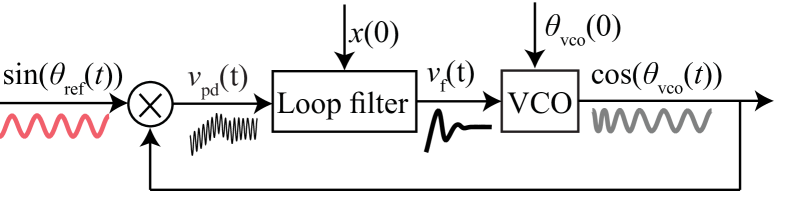
Figure 1: Classical PLL with multiplier and sinusoidal signals in the signal space.

Consider master-slave synchronization of oscillators by the classical PLL (see, e.g. [1]). Fig. 1 shows operation principle of classical PLL, without noise, in a signal space (the signal space model of PLL). Here the input is the signal of the reference oscillator $\sin(\theta_{\rm{ref}}(t))$ with phase $\theta_{\rm{ref}}(t)$ and instantaneous frequency $\dot{\theta}_{\rm{ref}}(t)=\omega_{\rm{ref}}(t)$. The signal of the voltage controlled oscillator (VCO) is $\cos(\theta_{\rm{vco}}(t))$ with phase $\theta_{\rm{vco}}(t)$ and instantaneous frequency $\dot{\theta}_{\rm{vco}}(t)=\omega_{\rm{vco}}(t)$. The multiplier generates a signal $v_{\rm{pd}}(t)=v_{e}(t)+v_{\rm{hf}}(t)$ which is the sum of the error signal $v_{e}(t)=\frac{1}{2}\sin(\theta_{\rm{ref}}(t)-\theta_{\rm{vco}}(t))$ and unwanted high-frequency signal $v_{\rm{hf}}(t)=\frac{1}{2}\cos(\theta_{\rm{ref}}(t)+\theta_{\rm{vco}}(t))$. The loop filter suppresses unwanted high-frequency oscillations and its output $v_{\rm f}(t)$ adjusts the free-running (quiescent) frequency $\omega^{\rm free}_{\rm vco}$ of the VCO to the frequency of the input signal. Similarly, operation with square waveform signals $\operatorname{sign}\sin(\theta_{\rm{ref}}(t))$ and $\operatorname{sign}\cos(\theta_{\rm{vco}}(t))$ can be considered. Initial state of the loop is $\theta_{\rm vco}(0)$ (initial phase shift of the VCO signal with respect to the reference signal) and $x(0)$ (initial state of the loop filter). For the reference signal with constant high frequency $\omega_{\rm{ref}}(t)\equiv\omega_{\rm{ref}}$ the loop can achieve only almost complete synchronization of the signals (because of non ideal filtration of high-frequency signal) when in a locked state $|\omega_{\rm vco}(t)-\omega_{\rm ref}|\leq\omega_{e}^{\rm max},\ |\theta_{e}(t)-\theta_{e}(0)|\leq\theta_{e}^{\rm max},\ t\geq 0,$ where constants $\omega_{e}^{\rm max}$ and $\theta_{e}^{\rm max}$ are determined by engineering requirements for a particular application.

Important issues in the design of PLL are (see, e.g. pioneering monographs [1, 2, 3], published in 1966, and a rather comprehensive bibliography of pioneering works in [4]): estimation of the ranges for deviation between oscillators’ frequencies for which a locked state can be achieved (i.e. the synchronization is possible), analysis of the locked states stability, and study of possible transient processes.

In [1] Floyd Gardner introduced a lock-in concept: “If, for some reason, the frequency difference between input and VCO is less than the loop bandwidth, the loop will lock up almost instantaneously without slipping cycles. The maximum frequency difference for which this fast acquisition is possible is called the lock-in frequency”. The above notion of lock-in frequency and corresponding definition of the lock-in range (called also a lock range[5, p.256], a seize range [6, p.138]) are given in various engineering publications. However, in general, even for zero frequency difference there may exist initial states of loop such that cycle slipping may take place. Thus, consideration of initial state of the loop is of utmost importance for the cycle slip analysis and, therefore, the original concept of lock-in frequency lacks rigor and requires clarification. In 1979 F. Gardner in the 2nd edition of his well-known work, Phaselock Techniques, [22, p.70] (see also the 3rd edition [23, p.187-188] published in 2005) wrote that “despite its vague reality, lock-in range is a useful concept” and formulated the following problem: “there is no natural way to define exactly any unique lock-in frequency”.

Recently a rigorous clarification of the lock-in range notion and solution to Gardner’s problem were suggested in [24, 25]. Below we suggest further extension of the lock-in range notion for the signal space PLL model.

Definition 1 (Pull-in and lock-in ranges).

For a certain free-running frequency of the VCO the largest symmetric interval, around zero, of the difference between the reference frequency and the free-running frequency of the VCO, such that for corresponding frequencies and arbitrary initial state the loop acquires a locked state, is called a pull-in range. If, in addition, the loop in a locked state after any abrupt change of the reference frequency within the interval acquires a locked state without cycle slipping, then the interval is called a lock-in range.

Further this definition is explained on the example of classical second-order PLL model in a signal’s phase space with lead-lag and active proportional-integral (PI) filters. An effective computational method for the lock-in frequency is discussed and corresponding estimates are obtained.

Figure 2: Classic analog PLL in the signal’s phase space.

II The signal’s phase space model

Following pioneering engineering publications [1, 2, 3], consider the operation of classical analog PLL in a signal’s phase space, where the phase changes of the signals are considered instead of the signals themselves. The averaging method [26, 27, 28, 29, 30, 31] allows to reduce the model in the signal space (see Fig. 1) to the model in the signal’s phase space (see Fig. 2) under certain conditions. Nowadays nonlinear model in Fig. 2 is widely used (see, e.g. [13, 35, 18]) to study acquisition processes of various circuits. In Fig. 2 the phases $\theta_{\rm ref,vco}(t)$ of the input (reference) and VCO signals are inputs of the nonlinear phase detector (PD) block. The output of PD is a function $v_{e}(\theta_{e}(t))$ (called PD characteristic), where

$$\theta_{e}(t)=\theta_{\rm{ref}}(t)-\theta_{\rm{vco}}(t)$$ (1)

is named the phase error. For the classical PLL with sinusoidal signals and a two-phase PLL we have

$$v_{e}(\theta_{e})=\frac{1}{2}\sin(\theta_{e}),$$ (2)

in case of square waveforms of reference and VCO signals $v_{e}(\theta_{e})$ has triangular waveform

$$v_{e}(\theta_{e})=\left\{\!\!\!\!\begin{array}[]{ll}\frac{2}{\pi}(\theta_{e}-2\pi),&\!\!\!\!\!\!\rm{if\ }(\theta_{e}{\,\rm mod\,}2\pi)\in[-\frac{\pi}{2},\frac{\pi}{2}]\\ 2-\frac{2}{\pi}(\theta_{e}-2\pi),&\!\!\!\!\rm{if\ }(\theta_{e}{\,\rm mod\,}2\pi)\in[\frac{\pi}{2},\frac{3}{2}\pi]\end{array}\right.$$ (3)

The relationship between the input $v_{e}(\theta_{e}(t))$ and the output $v_{f}(t)$ of the Loop filter is as follows:

$$\dot{x}=Ax+bv_{e}(\theta_{e}(t)),\ v_{\rm f}(t)=c^{*}x+hv_{e}(\theta_{e}(t)),$$ (4)

where $A$ is a constant $n\times n$ matrix, $x(t)\in\mathbb{R}^{n}$ is the filter state, $x(0)$ is the initial state of filter, $b$ and $c$ are constant vectors, and h is a number. The Loop filter transfer function has the form:

$$H(s)=-c^{*}(A-sI)^{-1}b+h,$$ (5)

where ^∗ is matrix transposition, $I$ is $n\times n$ unit matrix. A lead-lag filter or a PI filter [18] are usually used as the Loop filters. The control signal $v_{f}(t)$ adjusts the VCO frequency:

$$\dot{\theta}_{\rm{vco}}(t)=\omega_{\rm{vco}}(t)=\omega_{\rm{vco}}^{\text{free}}+K_{\rm vco}v_{f}(t),$$ (6)

where $\omega_{\rm{vco}}^{\text{free}}$ is the VCO free-running frequency and $K_{\rm vco}$ is the VCO gain. Nonlinear VCO models can be similarly considered, see, e.g. [40, 41, 42, 43]. The frequency of the input signal (reference frequency) is usually assumed to be constant:

$$\dot{\theta}_{\rm{ref}}(t)=\omega_{\rm{ref}}(t)\equiv\omega_{\rm{ref}}.$$ (7)

The difference between the reference frequency and the VCO free-running frequency is denoted as $\omega_{e}^{\text{free}}$:

$$\omega_{e}^{\text{free}}\equiv\omega_{\rm{ref}}-\omega_{\rm{vco}}^{\text{free}}.$$ (8)

By combining equations (1), (4), and (6)–(8) a nonlinear mathematical model in the signal’s phase space is obtained (i.e. in the state space: the filter’s state $x$ and the difference between the signal’s phases $\theta_{e}$):

$$\dot{x}=Ax+bv_{e}(\theta_{e}),$$ (9)

$$\dot{\theta}_{e}=\omega_{e}^{\text{free}}-K_{\rm vco}\big{(}c^{*}x+hv_{e}(\theta_{e})\big{)}.$$

Classical PD characteristics are bounded piecewise-smooth $2\pi$ periodic functions, thus it is convenient to assume that ($\theta_{e}$ mod $2\pi$) is a cyclic variable, and the analysis is restricted to the range of $\theta_{e}(0)\in[-\pi,\pi)$.

System (9) with an odd PD characteristic (i.e. $v_{e}(-\theta_{e})=-v_{e}(\theta_{e})$) is not changed by the transformation

$$\big{(}\omega_{e}^{\text{free}},x(t),\theta_{e}(t))\rightarrow\big{(}-\omega_{e}^{\text{free}},-x(t),-\theta_{e}(t)),$$ (10)

and it allows to study system (9) for $\omega_{e}^{\text{free}}>0$ only, introducing the concept of frequency deviation:

$$|\omega_{e}^{\text{free}}|=|\omega_{\rm{ref}}-\omega_{\rm{vco}}^{\text{free}}|.$$ (11)

II-A Pull-in and lock-in ranges

For nonlinear mathematical model in the signal’s phase space (9) we can consider the conditions of complete synchronization, i.e. the frequency error is zero and the phase error is constant:

$$\dot{\theta}_{e}(t)\equiv 0,\theta_{e}(t)\equiv\theta_{s}.$$ (12)

For most of the considered loop filters (i.e. controllable and observable) the above equation implies that filter state is also constant:

$$x(t)\equiv x_{s}.$$ (13)

Thus, in complete synchronization the locked states of the model in the signal’s phase space are the equilibrium points of system (9). The equilibrium points can be considered as a multiple-valued function of variable $\omega_{e}^{\text{free}}$: $\big{(}x_{s}(\omega_{e}^{\text{free}}),\theta_{s}(\omega_{e}^{\text{free}})\big{)}$. Note, that for all practically used phase detectors the characteristics $v_{e}(\theta_{e})$ (e.g. sinusoidal and triangular) have exactly one stable and one unstable equilibriua on each period.

An important characteristic of PLL is the set of $\omega_{e}^{\rm free}$ such that the model acquires locked state for any initial state.

Definition 2 (Pull-in range of the signal’s phase space model, see [24, 25, 45]).

The largest interval of frequency deviations $|\omega_{e}^{\rm free}|\in[0,\omega_{\text{pull-in}})$ such that the signal’s phase space model (9) acquires a locked state for arbitrary initial state $(x(0),\theta_{e}(0))$ is called a pull-in range, $\omega_{\text{pull-in}}$ is called a pull-in frequency.

Definition 3 (Cycle slipping).

Let PD characteristic $v_{e}(\theta_{e})$ be $2\pi$-periodic function. If

$$\sup\limits_{t>0}|\theta_{e}(0)-\theta_{e}(t)|\geq 2\pi$$ (14)

it is then said that cycle slipping occurs [46, p.131],[25]. Sometimes $\limsup\limits_{t\to+\infty}$ is considered instead of $\sup\limits_{t>0}$ in (14).

Further we consider only cycle slipping caused by deterministic dynamics [47, 1, 48, 49], noise-induced cycle slips are studied, e.g. in [50, 46, 51].

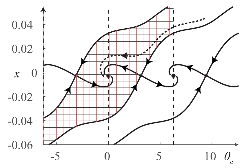
Figure 3: Phase portrait of the signal’s phase space model of the classical PLL with lead-lag filter: $H(s)=\frac{1+s\tau_{2}}{1+s\tau_{1}}$, $\tau_{1}=6.33\cdot 10^{-2}$, $\tau_{2}=1.85\cdot 10^{-2}$, $K_{\rm vco}=250$, $v_{e}(\theta_{e})=\frac{1}{2}\sin(\theta_{e})$, $\omega_{e}^{\text{free}}=0$. Dots are equilibria. Separatrices pass in and out of unstable saddle equilibria, outgoing separatrices tend to stable equilibria. The local lock-in domain, where trajectories tend to zero equilibrium without slipping cycles, is shaded. The dashed trajectory starts outside the lock-in domain and skips cycles.

The pull-in (or acquisition) process may take more than one beat note, i.e the VCO frequency will be slowly tuned toward the reference frequency and cycle slipping may take place. Remark that even for zero frequency deviation ($\omega_{e}^{\text{free}}=0$) and a sufficiently large initial state of filter $x(0)$ the cycle slipping may take place (see, e.g. dashed trajectory in Fig. 3). Thus, consideration of all state variables is of utmost importance for the cycle slipping analysis. A numerical study of cycle slipping for the classical PLL can be found in [52]. Analytical tools for estimating the number of cycle slips can be found, e.g. in [53, 48, 29].

Definition 4 (Lock-in range of the signal’s phase space model, see [24, 25, 45]).

The largest interval of frequency deviations from the pull-in range: $|\omega_{e}^{\rm free}|\in[0,\omega_{\text{lock-in}})\subset[0,\omega_{\text{pull-in}})$, is called a lock-in range if the signal’s phase space model (9), being in a locked state, after any abrupt change of $\omega_{e}^{\rm free}$ within the interval acquires a locked state without cycle slipping.

Remark that in contrast to the pull-in and lock-in ranges for the signal space model (see Definition 1, Fig. 1) the ranges for the signal’s phase space model (Fig. 2) depend only on the difference between frequencies $|\omega_{\rm{ref}}-\omega_{\rm{vco}}^{\text{free}}|$, but not on the frequencies $\omega_{\rm{ref}}$ and $\omega_{\rm{vco}}^{\text{free}}$ themselves. However, it must be remembered that reduction of the signal space model to the signal’s phase space model by the averaging is reliable only for sufficiently high frequencies.

Consider the behavior of trajectories (transient processes) of system (9) in the state space $(x,\theta)$ (see, e.g., the state space for a second-order model in Fig. 3). Each of the equilibrium states (locked states) has a vicinity in the state space, called a local lock-in domain, where corresponding trajectories tend to the locked state without slipping cycles (see, e.g. shaded local lock-in domain in Fig. 3 defined by corresponding ingoing separatrices of unstable equilibria). The lock-in domain is the union of local lock-in domains, each of which corresponds to one of the equilibria. The shape of the lock-in domain may vary significantly depending on $\omega_{e}^{\text{free}}$. We denote by ${\rm D}_{\text{lock-in}}(\omega_{e}^{\text{free}})$ lock-in domain corresponding to a specific frequency difference $\omega_{e}^{\text{free}}$. The above Definition 4 requires that the intersection of lock-in domains ${\rm D}_{\text{lock-in}}\big{(}(-\omega_{\text{lock-in}},\omega_{\text{lock-in}})\big{)}=\bigcap\limits_{|\omega_{e}^{\text{free}}|<\omega_{\text{lock-in}}}{\rm D}_{\text{lock-in}}(\omega_{e}^{\text{free}})$ contains all corresponding equilibria $\big{(}x_{s}(\omega_{e}^{\text{free}}),\theta_{s}(\omega_{e}^{\text{free}})\big{)}.$ Thus, after an abrupt change of frequencies, the model acquires a locked state without slipping cycles.

III Lock-in range of the classical analog PLL

To estimate numerically the lock-in range for the signal’s phase space model in Fig. 2, we can use, e.g., direct numerical integration of ordinary differential equation (9) in MATLAB or simulation of the signal’s phase space model in MATLAB Simulink.

With the usual numerical simulation or integration of dynamical model we can only observe transient processes (trajectories) toward the asymptotically stable locked states (equilibria), i.e. which are maintained under small perturbations of the phase difference and filter state; transient processes toward unstable locked states (see, e.g. ingoing separatrices of saddle equilibria in Fig. 3) cannot be obtained due to computational errors (caused by finite precision arithmetic and numerical approximation of ordinary differential equation solutions) and do not occur in real systems because of noise.

The usual numerical simulation allows observing transient processes (trajectories) toward the asymptotically stable locked states (equilibria) only, i.e. locked states which are maintained under small perturbations of the phase difference and filter state. Transient processes toward the unstable locked states (see, e.g. ingoing separatrices of saddle equilibria in Fig. 3) cannot be observed due to computational errors (caused by finite precision arithmetic and numerical approximation of ordinary differential equation solutions) and do not occur in real systems because of noise.

Without loss of generality we can fix $\omega_{\rm vco}^{\rm free}$ and vary $\omega_{\rm ref}$. Assume that the zero frequency deviation $\omega_{e}^{\text{free}}=0$ (i.e. the input frequency $\omega_{\rm{ref}}=\omega_{\rm vco}^{\rm free}$) belongs to the pull-in range and the model acquires an asymptotically stable locked state $(\theta_{s}^{0},x_{s}^{0})$ (without loss of generality we can consider $\theta^{0}_{s}=0$). First we abruptly increase the input frequency by sufficiently small frequency step $\Delta\omega>0$ (i.e. the input frequency becomes $\omega_{\rm ref}=\omega_{\rm vco}^{\rm free}+\Delta\omega$) and observe whether corresponding transient process converges to a locked state without cycle slipping (see Fig. 4). If $|\Delta\omega|$ belongs to the pull-in range then the model acquires new asymptotically stable locked state $(\theta^{+}_{s},x^{+}_{s})$ (otherwise we reduce $\Delta\omega$). If initial locked state belongs to the corresponding lock-in domain: $(\theta^{0}_{s},x^{0}_{s})\in{\rm D}_{\rm lock-in}(\Delta\omega)$, then the transient process from $(\theta^{0}_{s},x^{0}_{s})$ converges to the locked state $(\theta^{+}_{s},x^{+}_{s})$ without cycle slipping. Then we abruptly decrease the input frequency by $2\Delta\omega$, (i.e. the input frequency becomes $\omega_{\rm ref}=\omega_{\rm vco}^{\rm free}-\Delta\omega$). Since $|\Delta\omega|$ belongs to the pull-in range the model acquires new asymptotically stable locked state $(\theta^{-}_{s},x^{-}_{s})$. If the transient process converges from $(\theta^{+}_{s},x^{+}_{s})$ to the locked state $(\theta^{-}_{s},x^{-}_{s})$ without cycle slipping, (i.e. both symmetric locked states belong to the intersection of the lock-in domains: $(\theta_{s}^{\pm},x_{s}^{\pm})\in{\rm D}_{\rm lock-in}(|\Delta\omega|)={\rm D}_{\rm lock-in}(+\Delta\omega)\bigcap{\rm D}_{\rm lock-in}(-\Delta\omega)$), then we estimate the lock-in range as $[0,\Delta\omega]$.

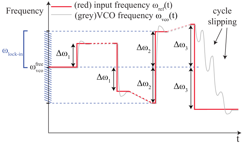
Figure 4: Estimation of the lock-in range.

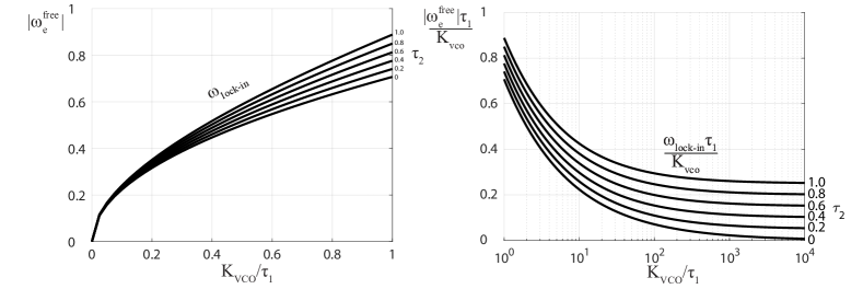
Figure 5: Lock-in frequency diagrams for model (15) (active PI filter) with sinusoidal phase detector characteristics (2). Left subfigure: $\omega_{\text{lock-in}}$ for $0<K_{\rm vco}/\tau_{1}<1$ in linear scale ($\omega_{\text{lock-in}}$ tends to $0$ as $K_{\rm vco}/\tau_{1}$ tends to 0). Right subfigure: $\frac{\omega_{\text{lock-in}}\tau_{1}}{K_{\rm vco}}$ for $K_{\rm vco}/\tau_{1}>1$ in logarithmic scale.

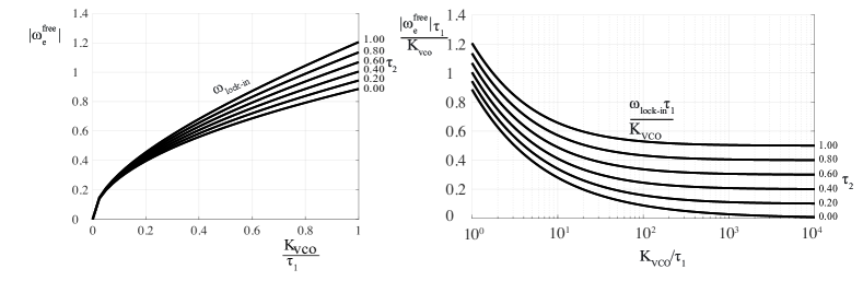
Figure 6: Lock-in frequency diagrams for model (15) (active PI filter) with triangular phase detector characteristics (3). Left subfigure: $\omega_{\text{lock-in}}$ for $0<K_{\rm vco}/\tau_{1}<1$ in linear scale ($\omega_{\text{lock-in}}$ tends to $0$ as $K_{\rm vco}/\tau_{1}$ tends to 0). Right subfigure: $\frac{\omega_{\text{lock-in}}\tau_{1}}{K_{\rm vco}}$ for $K_{\rm vco}/\tau_{1}>1$ in logarithmic scale.

Here we suppose that for a specific $\omega_{\rm ref}$ only one asymptotically stable locked state exist within a periodic interval: $(\theta_{s}^{\rm st}(\omega_{\rm ref}),x_{s}^{\rm st}(\omega_{\rm ref}))$, and for all $|\omega_{\rm ref}|<|\Delta\omega|$ we have $(\theta_{s}^{\rm st}(\omega_{\rm ref}),x_{s}^{\rm st}(\omega_{\rm ref}))\in{\rm D}_{\rm lock-in}(|\Delta\omega|).$ This allows investigating cycle slipping for a consecutive increases of frequency deviation $|\omega_{\rm ref}|$ only. Thus, simulation of all possible abrupt changes of frequency deviation within the lock-in range (see Fig. 4) is unnecessary.

The algorithm for computation of lock-in ranges used above doesn’t guarantee that the model acquires locked state for any initial filter state, i.e. lock-in range is not inside pull-in range automatically. To verify the global stability and estimate the pull-in range one can use the phase plane analysis (see, e.g. [56, 57, 58]) or a special modification of direct Lyapunov method for cylindrical phase space (see, e.g. [59, 48, 29, 25]). Some examples of the lock-in range computation by the phase plane analysis are presented in [25, 60, 61, 62, 63].

Below we provide complete solution of the Gardner problem on lock-in range computation for the classical second-order PLL with lead-lag and active proportional-integral (PI) filters, and sinusoidal and triangular PD characteristics.

III-A Active PI filter

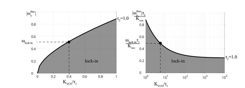
Figure 7: Lock-in range depending on $\frac{K_{\rm vco}}{\tau_{1}}$ (shaded domains) for model (15) (active PI filter) with sinusoidal phase detector characteristics (2) and $\tau_{2}=1$. Left subfigure: $\omega_{\text{lock-in}}$ for $0<K_{\rm vco}/\tau_{1}<1$ in linear scale. Right subfigure: $\frac{\omega_{\text{lock-in}}\tau_{1}}{K_{\rm vco}}$ for $K_{\rm vco}/\tau_{1}>1$ in logarithmic scale.

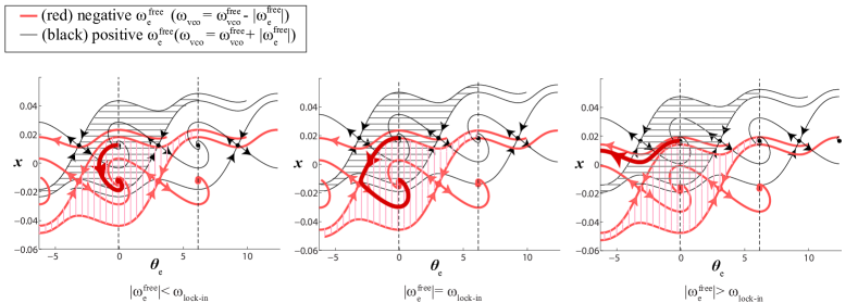
Figure 8: Phase portraits for model (15) with the following parameters: $H(s)=\frac{1+s\tau_{2}}{s\tau_{1}}$, $\tau_{1}=0.0633$, $\tau_{2}=0.0225$, $K_{\rm vco}=250$, $v_{e}(\theta_{e})=\frac{1}{2}\sin(\theta_{e})$. Black color is for the model with positive $\omega_{e}^{\text{free}}=|\widetilde{\omega}|$. Red is for the model with negative $\omega_{e}^{\text{free}}=-|\widetilde{\omega}|$. Equilibria (dots), separatrices pass in and out of the saddles equilibria, local lock-in domains are shaded (upper black horizontal lines are for $\omega_{e}^{\text{free}}>0$, lower red vertical lines are for $\omega_{e}^{\text{free}}<0$). Left subfig: $\omega_{e}^{\text{free}}=\pm 50$; middle subfig: $\omega_{e}^{\text{free}}=\pm 60$; right subfig: $\omega_{e}^{\text{free}}=\pm 66$.

Consider the PLL with the active PI loop filter (called “perfect PI”) having transfer function $H(s)=\frac{1+s\tau_{2}}{s\tau_{1}}$, where $\tau_{1},\tau_{2}>0$. The model (9) becomes

$$\dot{x}=\frac{v_{e}(\theta_{e})}{\tau_{1}},$$ (15)

$$\dot{\theta}_{e}=\omega_{e}^{\rm{free}}-K_{\rm{vco}}\bigg{(}x+\frac{\tau_{2}}{\tau_{1}}v_{e}(\theta_{e})\bigg{)}.$$

For PD characteristics (2) and (3) the model has one asymptotically stable $(0,-\frac{\omega_{e}^{\rm{free}}}{K_{\rm vco}})$ and one unstable $(\pi,-\frac{\omega_{e}^{\rm{free}}}{K_{\rm vco}})$ equilibrium points, which repeat on intervals of length $2\pi$. Note, that by the change of variables $(x\to x+\frac{\omega_{e}^{\rm{free}}}{K_{\rm vco}})$ in system (15) we get $\omega_{e}^{\rm{free}}\to 0$. Thus, a change of the parameter $\omega_{e}^{\text{free}}$ shifts the phase portrait vertically (in the variable $x$) without distorting trajectories, which simplifies the analysis of the lock-in domain and range (see Fig. 8). The pull-in range of model (15) is infinite.

For an arbitrary $\tau_{1}>0$ the following change of variables $x\to x/\tau_{1}$ reduces system (15) to the form

$$\dot{x}=v_{e}(\theta_{e}),$$ (16)

$$\dot{\theta}_{e}=\omega_{e}^{\rm{free}}-\frac{K_{\rm{vco}}}{\tau_{1}}\bigg{(}x+\tau_{2}v_{e}(\theta_{e})\bigg{)}.$$

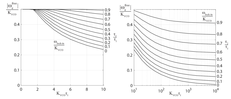
Figure 9: Lock-in frequency diagrams for model (19) (lead-lag filter) with sinusoidal phase detector characteristics (2). Left subfigure: $\frac{\omega_{\text{lock-in}}}{K_{\rm vco}}$ for $0<K_{\rm vco}\tau_{1}<10$ in linear scale ($\frac{\omega_{\text{lock-in}}}{K_{\rm vco}}$ tends to $1/2$ as $K_{\rm vco}\tau_{1}$ tends to 0). Right subfigure: $\frac{\omega_{\text{lock-in}}}{K_{\rm vco}}$ for $K_{\rm vco}\tau_{1}>10$ in logarithmic scale.

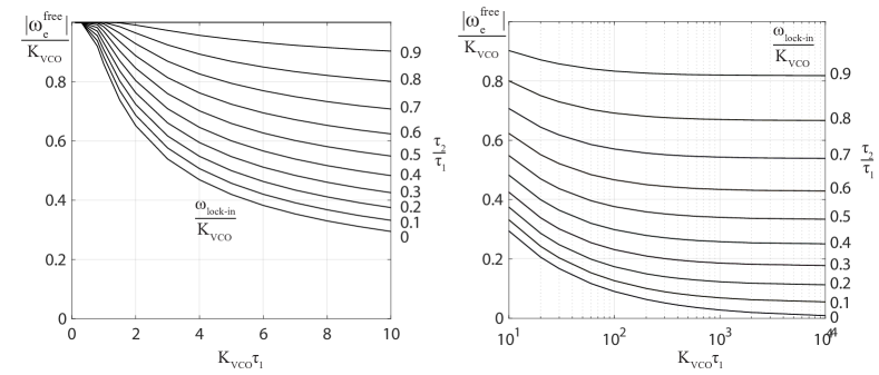
Figure 10: Lock-in frequency diagrams for model (19) (lead-lag filter) with triangular phase detector characteristics (3). Left subfigure: $\frac{\omega_{\text{lock-in}}}{K_{\rm vco}}$ for $0<K_{\rm vco}\tau_{1}<10$ in linear scale ($\frac{\omega_{\text{lock-in}}}{K_{\rm vco}}$ tends to $1$ as $K_{\rm vco}\tau_{1}$ tends to 0). Right subfigure: $\frac{\omega_{\text{lock-in}}}{K_{\rm vco}}$ for $K_{\rm vco}\tau_{1}>10$ in logarithmic scale.

This change of variables rescales the phase portrait of the system (see Fig. 3) and, thus, does not affect the stability and cycle slipping properties of the trajectories. Therefore, $\omega_{\text{lock-in}}$ can be found as a function of $\tau_{2},K_{\rm vco}/\tau_{1}$. For model (15) with phase detector characteristics (2) and (3) the lock-in frequency diagrams as function of $\tau_{2}$ (for $\tau_{2}\in[0,1]$) and $K_{\rm vco}/\tau_{1}$ are shown in Fig. 5 and Fig. 6, respectively. To determine the lock-in frequency $\omega_{\text{lock-in}}=\omega_{\text{lock-in}}(\tau_{2},K_{\rm vco}/\tau_{1})$ by diagrams in Fig. 5 and Fig. 6 one has to choose a curve corresponding to the loop filter parameter $\tau_{2}\in[0,1]$, select a point on the curve with the abscissa equal to $\frac{K_{\rm vco}}{\tau_{1}}$, and then corresponding ordinate in the left subfigure and product of the ordinates by $\frac{K_{\rm vco}}{\tau_{1}}$ in the right subfigure gives the lock-in frequency $\omega_{\text{lock-in}}$ (see Fig. 7).

Note, that for arbitrary $\tau_{2}>0$ by the following change of variables $t\to t\tau_{2},x\to x\tau_{2}$ in system (16) we get $\omega_{e}^{\rm{free}}\to\tau_{2}\omega_{e}^{\rm{free}},K_{\rm{vco}}\to\tau_{2}^{2}K_{\rm{vco}}/\tau_{1}$ (the considered time reparametrisation does not affect the cycle slipping property (14) of trajectories). Therefore, $\omega_{\text{lock-in}}(\tau_{2},K_{\rm vco})$ for $\tau_{2}>1$ can be computed from the diagrams in Fig. 5 and Fig. 6 by the formula:

$$\omega_{\text{lock-in}}(\tau_{2},K_{\rm vco}/\tau_{1})=\omega_{\text{lock-in}}(1,K_{\rm{vco}}\tau_{2}^{2}/\tau_{1})/\tau_{2}.$$ (17)

In [62, 61] a method for analytical computation of separatrices in model (15) is developed, which allows us to get the following lock-in frequency estimate

$$\omega_{\text{lock-in}}(\tau_{2},K_{\rm vco}/\tau_{1})\approx$$ (18)

$$\frac{1}{\sqrt{2}}\bigg{(}\frac{K_{\rm vco}}{\tau_{1}}\bigg{)}^{\frac{1}{2}}+\frac{1}{6}\frac{K_{\rm vco}}{\tau_{1}}+\frac{\tau_{2}^{2}(5-6\ln 2)}{\sqrt{2}\,36\tau_{1}}\bigg{(}\frac{K_{\rm vco}}{\tau_{1}}\bigg{)}^{\frac{3}{2}}.$$

Fig. (8) shows the phase portraits of model (15) with phase detector characteristics (2) when increasing the parameter $\omega_{\rm{ref}}$ in the computation of the lock-in range.

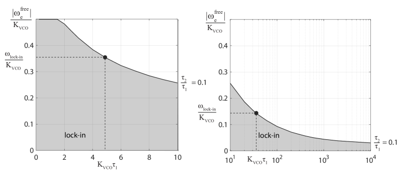
Figure 11: Lock-in range depending on $K_{\rm vco}\tau_{1}$ (shaded domains) for model (19) (lead-lag filter) with sinusoidal phase detector characteristics (2) and $\tau_{2}/\tau_{1}=0.1$. Left subfigure: $\frac{\omega_{\text{lock-in}}}{K_{\rm vco}}$ for $0<K_{\rm vco}\tau_{1}<10$ in linear scale. Right subfigure: $\frac{\omega_{\text{lock-in}}}{K_{\rm vco}}$ for $K_{\rm vco}\tau_{1}>10$ in logarithmic scale.

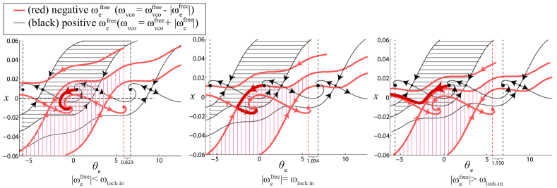
Figure 12: Phase portraits for model (19) with the following parameters: $H(s)=\frac{1+s\tau_{2}}{1+s\tau_{1}}$, $\tau_{1}=6.33\cdot 10^{-2}$, $\tau_{2}=1.85\cdot 10^{-2}$, $K_{\rm vco}=250$, $v_{e}(\theta_{e})=\frac{1}{2}\sin(\theta_{e})$. Black color is for the model with positive $\omega_{e}^{\text{free}}=|\widetilde{\omega}|$. Red is for the model with negative $\omega_{e}^{\text{free}}=-|\widetilde{\omega}|$. Equilibria (dots), separatrices pass in and out of the saddles equilibria, local lock-in domains are shaded (upper black horizontal lines are for $\omega_{e}^{\text{free}}>0$, lower red vertical lines are for $\omega_{e}^{\text{free}}<0$). Left subfig: $\omega_{e}^{\text{free}}=\pm 50$; middle subfig: $\omega_{e}^{\text{free}}=\pm 65$; right subfig: $\omega_{e}^{\text{free}}=\pm 68$.

III-B Lead-lag filter

Consider the PLL with passive lead-lag loop filter having transfer function $H(s)=\frac{1+s\tau_{2}}{1+s\tau_{1}}$, where $\tau_{1}>\tau_{2}\geq 0$. The model (9) becomes

$$\dot{x}=-\frac{1}{\tau_{1}}x+\frac{v_{e}(\theta_{e}(t))}{\tau_{1}},$$ (19)

$$\dot{\theta}_{e}=\omega_{e}^{\rm{free}}-K_{\rm{vco}}\bigg{(}\Big{(}1-\frac{\tau_{2}}{\tau_{1}}\Big{)}x+\frac{\tau_{2}}{\tau_{1}}v_{e}(\theta_{e}(t))\bigg{)}.$$

Model (19) with PD characteristic (2) for $\omega_{e}^{\rm{free}}<K_{\rm vco}/2$ has one asymptotically stable $\Big{(}\sin^{-1}\left(\frac{2\omega_{e}^{\rm{free}}}{K_{\rm vco}}\right),-\frac{\omega_{e}^{\rm{free}}}{K_{\rm vco}}\Big{)}$ and one unstable $\Big{(}\pi~{}-~{}\sin^{-1}\left(\frac{2\omega_{e}^{\rm{free}}}{K_{\rm vco}}\right),-\frac{\omega_{e}^{\rm{free}}}{K_{\rm vco}}\Big{)}$; and with PD characteristic (3) for $\omega_{e}^{\rm{free}}<K_{\rm vco}$ has one asymptotically stable equilibrium $\Big{(}\frac{\pi}{2}\frac{\omega_{e}^{\rm{free}}}{K_{\rm vco}},-\frac{\omega_{e}^{\rm{free}}}{K_{\rm vco}}\Big{)}$ and one unstable equilibrium $\Big{(}\frac{\pi}{2}\left(\frac{\omega_{e}^{\rm{free}}}{K_{\rm vco}}-2\right),-\frac{\omega_{e}^{\rm{free}}}{K_{\rm vco}}\Big{)}$. Thus, the pull-in range of model (19) loop filter is bounded. It can be estimated by the phase plane analysis or numerical computation (see corresponding diagram in [66, 29]), one of the difficulties of its computation caused by the so-called hidden oscillations [67, 25, 39]. The computed

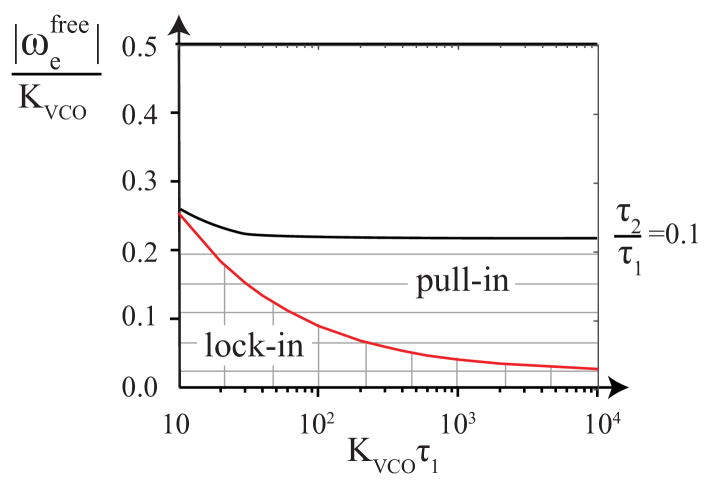
Figure 13: Pull-in and lock-in ranges depending on $K_{\rm vco}\tau_{1}$ (shaded domains) for model (19) (lead-lag filter) with sinusoidal phase detector characteristics (2) and $\tau_{2}/\tau_{1}=0.1$.

above values of the lock-in frequency are less than corresponding values of the pull-in frequency (see Fig. 13).

For an arbitrary $\tau_{1}>0$ the time reparametrization $t\to t\tau_{1}>0$ reduces system (19) to the form

$$\dot{x}=-x+v_{e}(\theta_{e}),$$ (20)

$$\dot{\theta}_{e}=\tau_{1}\omega_{e}^{\rm{free}}-\tau_{1}K_{\rm{vco}}\bigg{(}\Big{(}1-\frac{\tau_{2}}{\tau_{1}}\Big{)}x+\frac{\tau_{2}}{\tau_{1}}v_{e}(\theta_{e}(t))\bigg{)},$$

where $\tilde{\omega}_{e}^{\rm{free}}=\tau_{1}\omega_{e}^{\rm{free}}$ depends on two parameters: $\tau_{1}K_{\rm{vco}}$ and $\tau_{2}/\tau_{1}$.

For model (19) with phase detector characteristics (2) and (3) the lock-in frequency diagrams as function of $\tau_{2}/\tau_{1}$ (for $\tau_{2}/\tau_{1}\in[0,1]$) and $K_{\rm vco}\tau_{1}$ are shown in Fig. 9 and Fig. 10, respectively. To determine the lock-in frequency $\omega_{\text{lock-in}}=\omega_{\text{lock-in}}(\tau_{2}/\tau_{1},K_{\rm vco}\tau_{1})$ by diagrams in Fig. 9 and Fig. 10 one has to choose a curve corresponding to the loop filter parameters $\tau_{2}/\tau_{1}\in[0,1]$, select a point on the curve with abscissa equal to $K_{\rm vco}\tau_{1}$, and then the product of the ordinates by $K_{\rm vco}$ gives the lock-in frequency $\omega_{\text{lock-in}}$ (see Fig. 11).

Fig. (12) shows phase portraits of model (19) with phase detector characteristics (2) when increasing the parameter $\omega_{\rm{ref}}$ in the computation of the lock-in range.

Conclusion

Various PLL-based circuits (see, e.g. optical Costas loop used in intersatellite communication, BPSK Costas loop, two-phase Costas loop, two-phase PLL and others [37, 38, 18, 30, 34, 68, 45, 39, 21]) are represented in the signal’s phase space by the model in Fig. 2 and, thus, their lock-in ranges can be estimated by the above diagrams. Remark that the change of variables $(\theta_{e},x)\to(\theta_{e}/K_{\rm p},K_{\rm pd}x)$ transforms the model (9) with PD characteristic $K_{\rm pd}v_{e}\big{(}K_{p}\theta_{e}(t)\big{)}$ to the from with PD characteristics $v_{e}(\theta_{e}(t))$ (i.e. with $K_{\rm p}\to 1,K_{\rm pd}\to 1$) and $\omega_{e}^{\rm free}\to K_{\rm p}\omega_{e}^{\rm free},K_{\rm vco}\to K_{\rm p}K_{\rm pd}K_{\rm vco}$. Thus, the lock-in frequency for the model with active PI loop filter can be computed from the diagrams in Fig. 5 and Fig. 6 as $\omega_{\text{lock-in}}(\tau_{2},K_{\rm p}K_{\rm pd}K_{\rm vco}/\tau_{1})/K_{\rm p}$ and for the model with lead-lag loop filter can be computed from diagrams in Fig. 9 and Fig. 10 as $\omega_{\text{lock-in}}(\tau_{2}/\tau_{1},K_{\rm p}K_{\rm pd}K_{\rm vco}\tau_{1})/K_{\rm p}$. Analytical estimates of the lock-in range for two-dimensional models can be obtained by the Andronov point-transformation method [56] and the study of separatrices in cylindrical phase space (some estimations of separatrices for the classical PLL can be found in [57, 58, 2, 69, 23, 70]). For the second-order PLL with PI filter and triangular phase-detector characteristic an analytical estimate of the lock-in range can be found in [61, 62, 63].

Nikolay Kuznetsov received his Candidate degree from Saint-Petersburg State University (2004), Ph.D. from the University of Jyväskylä (2008), and D. Sc. from Saint-Petersburg State University (2016). He is currently Professor and Deputy Head of the Department of Applied Cybernetics at Saint-Petersburg State University, Visiting Professor at the University of Jyväskylä, and member of the MERLIN international research group at the Ton Duc Thang University. His interests are now in dynamical systems stability and oscillations, Lyapunov exponent, chaos, hidden attractors, phase-locked loop nonlinear analysis, nonlinear control systems. E-mail: nkuznetsov239@gmail.com (corresponding author)

Gennady Leonov received his Candidate degree in 1971 and D. Sc. in 1983 from Saint-Petersburg State University. In 1986 he was awarded the USSR State Prize for development of the theory of phase synchronization for radiotechnics and communications. Since 1988 he has been Dean of the Faculty of Mathematics and Mechanics at Saint-Petersburg State University and since 2007 Head of the Department of Applied Cybernetics. He is member (corresponding) of the Russian Academy of Science, in 2011 he was elected to the IFAC Council. His research interests are now in control theory and dynamical systems.

Marat Yuldashev received his Candidate degree from St.Petersburg State University (2013) and Ph.D. from the University of Jyväskylä (2013). He is currently at Saint-Petersburg University. His research interests cover nonlinear models of phase-locked loops and Costas loops, and SPICE simulation.

Renat Yuldashev received his Candidate degree from St.Petersburg State University (2013) and Ph.D. from the University of Jyväskylä (2013). He is currently at Saint-Petersburg University. His research interests cover nonlinear models of phase-locked loops and Costas loops, and simulation in MatLab Simulink.

References

- [1] F. Gardner, Phaselock techniques. New York: John Wiley & Sons, 1966.
- [2] V. Shakhgil’dyan and A. Lyakhovkin, Fazovaya avtopodstroika chastoty (in Russian). Moscow: Svyaz’, 1966.
- [3] A. Viterbi, Principles of coherent communications. New York: McGraw-Hill, 1966.
- [4] W. Lindsey and R. Tausworthe, A Bibliography of the Theory and Application of the Phase-lock Principle, ser. JPL technical report. Jet Propulsion Laboratory, California Institute of Technology, 1973.
- [5] K. Yeo, M. Do, and C. Boon, Design of CMOS RF Integrated Circuits and Systems. World Scientific, 2010.
- [6] W. Egan, Phase-Lock Basics. Wiley-IEEE Press, 2007.
- [7] R. Best, Phase-locked Loops: Design, Simulation, and Applications. McGraw Hill, 1984.
- [8] D. Wolaver, Phase-locked Loop Circuit Design. Prentice Hall, 1991.
- [9] G.-C. Hsieh and J. Hung, “Phase-locked loop techniques. A survey,” Industrial Electronics, IEEE Transactions on, vol. 43, no. 6, pp. 609–615, 1996.
- [10] J. Irwin, The Industrial Electronics Handbook. Taylor & Francis, 1997.
- [11] J. Craninckx and M. Steyaert, Wireless CMOS Frequency Synthesizer Design. Springer, 1998.
- [12] M. Kihara, S. Ono, and P. Eskelinen, Digital Clocks for Synchronization and Communications. Artech House, 2002.
- [13] D. Abramovitch, “Phase-locked loops: A control centric tutorial,” in American Control Conf. Proc., vol. 1. IEEE, 2002, pp. 1–15.
- [14] B. De Muer and M. Steyaert, CMOS Fractional-N Synthesizers: Design for High Spectral Purity and Monolithic Integration. Springer, 2003.
- [15] S. Dyer, Wiley Survey of Instrumentation and Measurement. Wiley, 2004.
- [16] K. Shu and E. Sanchez-Sinencio, CMOS PLL synthesizers: analysis and design. Springer, 2005.
- [17] S. Goldman, Phase-Locked Loops Engineering Handbook for Integrated Circuits. Artech House, 2007.
- [18] R. Best, Phase-Locked Loops: Design, Simulation and Application, 6th ed. McGraw-Hill, 2007.
- [19] R. Baker, CMOS: Circuit Design, Layout, and Simulation, ser. IEEE Press Series on Microelectronic Systems. Wiley-IEEE Press, 2011.
- [20] V. Kroupa, Frequency Stability: Introduction and Applications, ser. IEEE Series on Digital & Mobile Communication. Wiley-IEEE Press, 2012.
- [21] R. Middlestead, Digital Communications with Emphasis on Data Modems: Theory, Analysis, Design, Simulation, Testing, and Applications. Wiley, 2017.
- [22] F. Gardner, Phaselock techniques, 2nd ed. New York: John Wiley & Sons, 1979.
- [23] ——, Phaselock Techniques, 3rd ed. Wiley, 2005.
- [24] N. Kuznetsov, G. Leonov, M. Yuldashev, and R. Yuldashev, “Rigorous mathematical definitions of the hold-in and pull-in ranges for phase-locked loops,” IFAC-PapersOnLine, vol. 48, no. 11, pp. 710–713, 2015. 10.1016/j.ifacol.2015.09.272
- [25] G. Leonov, N. Kuznetsov, M. Yuldashev, and R. Yuldashev, “Hold-in, pull-in, and lock-in ranges of PLL circuits: rigorous mathematical definitions and limitations of classical theory,” IEEE Transactions on Circuits and Systems–I: Regular Papers, vol. 62, no. 10, pp. 2454–2464, 2015. 10.1109/TCSI.2015.2476295
- [26] N. Krylov and N. Bogolyubov, Introduction to non-linear mechanics. Princeton: Princeton Univ. Press, 1947.
- [27] J. Kudrewicz and S. Wasowicz, Equations of phase-locked loop. Dynamics on circle, torus and cylinder. World Scientific, 2007.
- [28] G. Leonov, N. Kuznetsov, M. Yuldahsev, and R. Yuldashev, “Analytical method for computation of phase-detector characteristic,” IEEE Transactions on Circuits and Systems - II: Express Briefs, vol. 59, no. 10, pp. 633–647, 2012. 10.1109/TCSII.2012.2213362
- [29] G. Leonov and N. Kuznetsov, Nonlinear Mathematical Models of Phase-Locked Loops. Stability and Oscillations. Cambridge Scientific Publisher, 2014.
- [30] G. Leonov, N. Kuznetsov, M. Yuldashev, and R. Yuldashev, “Nonlinear dynamical model of Costas loop and an approach to the analysis of its stability in the large,” Signal Processing, vol. 108, pp. 124–135, 2015. 10.1016/j.sigpro.2014.08.033
- [31] ——, “Computation of the phase detector characteristic of a QPSK Costas loop,” Doklady Mathematics, vol. 93, no. 3, pp. 348–353, 2016. 10.1134/S1064562416030236
- [32] J. Piqueira and L. Monteiro, “Considering second-harmonic terms in the operation of the phase detector for second-order phase-locked loop,” IEEE Transactions On Circuits And Systems-I, vol. 50, no. 6, pp. 805–809, 2003.
- [33] N. Kuznetsov, O. Kuznetsova, G. Leonov, P. Neittaanmaki, M. Yuldashev, and R. Yuldashev, “Limitations of the classical phase-locked loop analysis,” Proceedings - IEEE International Symposium on Circuits and Systems, vol. 2015-July, pp. 533–536, 2015. 10.1109/ISCAS.2015.7168688
- [34] R. Best, N. Kuznetsov, O. Kuznetsova, G. Leonov, M. Yuldashev, and R. Yuldashev, “A short survey on nonlinear models of the classic Costas loop: rigorous derivation and limitations of the classic analysis,” in Proceedings of the American Control Conference. IEEE, 2015, pp. 1296–1302, art. num. 7170912. 10.1109/ACC.2015.7170912
- [35] D. Abramovitch, “Method for guaranteeing stable non-linear PLLs,” 2004, US Patent App. 10/414,791, http://www.google.com/patents/US20040208274.
- [36] N. Kuznetsov, G. Leonov, S. Seledzhi, M. Yuldashev, and R. Yuldashev, “Elegant analytic computation of phase detector characteristic for non-sinusoidal signals,” IFAC-PapersOnLine, vol. 48, no. 11, pp. 960–963, 2015. 10.1016/j.ifacol.2015.09.316
- [37] T. Emura, L. Wang, M. Yamanaka, and H. Nakamura, “A high-precision positioning servo controller based on phase/frequency detecting technique of two-phase-type PLL,” Industrial Electronics, IEEE Transactions on, vol. 47, no. 6, pp. 1298–1306, 2000.
- [38] R. Best, N. Kuznetsov, G. Leonov, M. Yuldashev, and R. Yuldashev, “Simulation of analog Costas loop circuits,” International Journal of Automation and Computing, vol. 11, no. 6, pp. 571–579, 2014. 10.1007/s11633-014-0846-x
- [39] N. Kuznetsov, G. Leonov, M. Yuldashev, and R. Yuldashev, “Hidden attractors in dynamical models of phase-locked loop circuits: limitations of simulation in MATLAB and SPICE,” Commun Nonlinear Sci Numer Simulat, vol. 51, pp. 39–49, 2017. 10.1016/j.cnsns.2017.03.010
- [40] N. Margaris, Theory of the Non-Linear Analog Phase Locked Loop. New Jersey: Springer Verlag, 2004.
- [41] A. Suarez, Analysis and Design of Autonomous Microwave Circuits, ser. Wiley Series in Microwave and Optical Engineering. Wiley-IEEE Press, 2009.
- [42] M. Bonnin, F. Corinto, and M. Gilli, “Phase noise, and phase models: Recent developments, new insights and open problems,” Nonlinear Theory and Its Applications, IEICE, vol. 5, no. 3, pp. 365–378, 2014. 10.1587/nolta.5.365
- [43] G. Bianchi, N. Kuznetsov, G. Leonov, S. Seledzhi, M. Yuldashev, and R. Yuldashev, “Hidden oscillations in SPICE simulation of two-phase Costas loop with non-linear VCO,” IFAC-PapersOnLine, vol. 49, no. 14, pp. 45–50, 2016. 10.1016/j.ifacol.2016.07.973
- [44] I. A. Mitropolsky, “Averaging method in non-linear mechanics,” International Journal of Non-Linear Mechanics, vol. 2, no. 1, pp. 69–96, 1967.
- [45] R. Best, N. Kuznetsov, G. Leonov, M. Yuldashev, and R. Yuldashev, “Tutorial on dynamic analysis of the Costas loop,” Annual Reviews in Control, vol. 42, pp. 27–49, 2016. 10.1016/j.arcontrol.2016.08.003
- [46] J. Stensby, Phase-Locked Loops: Theory and Applications, ser. Phase-locked Loops: Theory and Applications. Taylor & Francis, 1997.
- [47] J. J. Stoker, Nonlinear Vibrations in Mechanical and Electrical Systems. N.Y: L.: Interscience, 1950.
- [48] G. A. Leonov, V. Reitmann, and V. B. Smirnova, Nonlocal Methods for Pendulum-like Feedback Systems. Stuttgart-Leipzig: Teubner Verlagsgesselschaft, 1992.
- [49] V. Smirnova and A. Proskurnikov, “Phase locking, oscillations and cycle slipping in synchronization systems,” in 2016 European Control Conference Proceedings, 2016, pp. 873–878. 10.1109/ECC.2016.7810399
- [50] V. Tikhonov, “Noise influence on operation of frequency phase adjustment circuit,” Automatika i Telemekhanika (in Russian), vol. 20, no. 9, pp. 1188–1196, 1959.
- [51] D. Talbot, Frequency Acquisition Techniques for Phase Locked Loops. Wiley-IEEE Press, 2012.
- [52] G. Ascheid and H. Meyr, “Cycle slips in phase-locked loops: A tutorial survey,” Communications, IEEE Transactions on, vol. 30, no. 10, pp. 2228–2241, 1982.
- [53] O. B. Ershova and G. A. Leonov, “Frequency estimates of the number of cycle slidings in phase control systems,” Avtomat. Remove Control, vol. 44, no. 5, pp. 600–607, 1983.
- [54] U. Meyer-Baese, Digital Signal Processing with Field Programmable Gate Arrays. Springer, 2004.
- [55] G. Bianchi, N. Kuznetsov, G. Leonov, M. Yuldashev, and R. Yuldashev, “Limitations of PLL simulation: hidden oscillations in MATLAB and SPICE,” International Congress on Ultra Modern Telecommunications and Control Systems and Workshops (ICUMT 2015), vol. 2016-January, pp. 79–84, 2016. 10.1109/ICUMT.2015.7382409
- [56] A. A. Andronov, E. A. Vitt, and S. E. Khaikin, Theory of Oscillators (in Russian). ONTI NKTP SSSR, 1937, [English transl.: 1966, Pergamon Press].
- [57] N. A. Gubar’, “Investigation of a piecewise linear dynamical system with three parameters,” J. Appl. Math. Mech., vol. 25, no. 6, pp. 1011–1023, 1961.
- [58] B. Shakhtarin, “Study of a piecewise-linear system of phase-locked frequency control,” Radiotechnica and electronika (in Russian), no. 8, pp. 1415–1424, 1969.
- [59] A. Gelig, G. Leonov, and V. Yakubovich, Stability of Nonlinear Systems with Nonunique Equilibrium (in Russian). Nauka, 1978, (English transl: Stability of Stationary Sets in Control Systems with Discontinuous Nonlinearities, 2004, World Scientific).
- [60] M. Blagov, E. Kudryashova, N. Kuznetsov, G. Leonov, M. Yuldashev, and R. Yuldashev, “Computation of lock-in range for classic pll with lead-lag filter and impulse signals,” IFAC-PapersOnLine, vol. 49, no. 14, pp. 42–44, 2016. 10.1016/j.ifacol.2016.07.972
- [61] K. Aleksandrov, N. Kuznetsov, G. Leonov, N. Neittaanmaki, M. Yuldashev, and R. Yuldashev, “Computation of the lock-in ranges of phase-locked loops with PI filter,” IFAC-PapersOnLine, vol. 49, no. 14, pp. 36–41, 2016. 10.1016/j.ifacol.2016.07.971
- [62] K. Aleksandrov, N. Kuznetsov, G. Leonov, M. Yuldashev, and R. Yuldashev, “Lock-in range of PLL-based circuits with proportionally-integrating filter and sinusoidal phase detector characteristic,” arXiv preprint arXiv:1603.08401, 2016.
- [63] ——, “Lock-in range of classical PLL with impulse signals and proportionally-integrating filter,” arXiv preprint arXiv:1603.09363, 2016.
- [64] Y. N. Bakaev, “Stability and dynamical properties of astatic frequency synchronization system,” Radiotekhnika i Elektronika (in Russian), vol. 8, no. 3, pp. 513–516, 1963.
- [65] K. Alexandrov, N. Kuznetsov, G. Leonov, P. Neittaanmaki, and S. Seledzhi, “Pull-in range of the PLL-based circuits with proportionally-integrating filter,” IFAC-PapersOnLine, vol. 48, no. 11, pp. 720–724, 2015. 10.1016/j.ifacol.2015.09.274
- [66] L. Belyustina, V. Brykov, K. Kiveleva, and V. Shalfeev, “On the magnitude of the locking band of a phase-shift automatic frequency control system with a proportionally integrating filter,” Radiophysics and Quantum Electronics, vol. 13, no. 4, pp. 437–440, 1970.
- [67] G. Leonov and N. Kuznetsov, “Hidden attractors in dynamical systems. From hidden oscillations in Hilbert-Kolmogorov, Aizerman, and Kalman problems to hidden chaotic attractors in Chua circuits,” International Journal of Bifurcation and Chaos, vol. 23, no. 1, 2013, art. no. 1330002. 10.1142/S0218127413300024
- [68] W. Rosenkranz and S. Schaefer, “Receiver design for optical inter-satellite links based on digital signal processing,” in Transparent Optical Networks (ICTON), 2016 18th International Conference on. IEEE, 2016, pp. 1–4.
- [69] V. D. Shalfeev and V. V. Matrosov, Nonlinear dynamics of phase synchronization systems (in Russian). Nizhni Novgorod University Press, 2013.
- [70] A. S. Huque and J. Stensby, “An analytical approximation for the pull-out frequency of a PLL employing a sinusoidal phase detector,” ETRI Journal, vol. 35, no. 2, pp. 218–225, 2013.