Improving the IMEX method with a residual balanced decomposition

Abstract

In numerical time-integration with implicit-explicit (IMEX) methods, a within-step adaptable decomposition called residual balanced decomposition is introduced. With this decomposition, the requirement of a small enough residual in the iterative solver can be removed, consequently, this allows to exchange stability for efficiency. This decomposition transfers any residual occurring in the implicit equation of the implicit-step into the explicit part of the decomposition. By balancing the residual, the accuracy of the local truncation error of the time-stepping method becomes independent from the accuracy by which the implicit equation is solved. In order to balance the residual, the original IMEX decomposition is adjusted after the iterative solver has been stopped. For this to work, the traditional IMEX time-stepping algorithm needs to be changed. We call this new method the shortcut-IMEX (SIMEX). SIMEX can gain computational efficiency by exploring the trade-off between the computational effort placed in solving the implicit equation and the size of the numerically stable time-step. Typically, increasing the number of solver iterations increases the largest stable step-size. Both multi-step and Runge-Kutta (RK) methods are suitable for use with SIMEX. Here, we show the efficiency of a SIMEX-RK method in overcoming parabolic stiffness by applying it to a nonlinear reaction-advection-diffusion equation. In order to define a stability region for SIMEX, a region in the complex plane is depicted by applying SIMEX to a suitable PDE model containing diffusion and dispersion. A myriad of stability regions can be reached by changing the RK tableau and the solver.

65L06, 65M20, 65L04

1 Introduction

Stiff ODEs are present in many applications, notably when the method of lines is used for the semi-discretization of PDEs. Both the parabolic stiffness due to diffusion and the hyperbolic stiffness due to the CFL condition are common sources of stiffness in PDEs. Stiffness imposes small time-step sizes in order to avoid numerical instabilities. In general, implicit time-stepping allows a larger time-step size but it requires the solution of an implicit equation at every step/stage of the method. IMEX methods decompose the right-hand-side of the ODE as the sum of two functions

(1) $$\frac{d{\mathbf{y}}}{dt}={\mathbf{f}}({\mathbf{y}},t)+{\mathbf{g}}({\mathbf{y}},t),$$

where ${\mathbf{f}}$ is the explicit part of the decomposition and ${\mathbf{g}}$ is the implicit part. An efficient decomposition should place non-stiff terms in ${\mathbf{f}}$ and stiff terms in ${\mathbf{g}}$ while keeping the implicit equation simple to solve. For IMEX, there is the restriction that the implicit equation needs to be solved up to a given precision in order to avoid introducing errors that could overwhelm the local truncation error; i.e., there is a small-enough-residual restriction to be fulfilled. The objective of the present article is to remove this restriction.

A new method called shortcut-IMEX (SIMEX) is introduced. It allows an iterative solver applied to the implicit equations to be interrupted at a given iteration. The reason SIMEX does not introduce errors is the use of a residual balanced decomposition: after the iterative solver is interrupted, any remaining residual of the implicit equation is accounted for in the explicit time-step by a suitable redefinition of the implicit-explicit decomposition. This within-step adjustment of the decomposition requires a modification of traditional algorithms used with IMEX. Many IMEX time-integrators can be adapted to SIMEX; namely, singly-diagonally-implicit Runge-Kutta schemes (SDIRK), explicit first stage SDIRK schemes (ESDIRK) [1, 2, 6, 19, 27, 28, 31, 34, 39, 40, 42], some general-linear-methods (IMEX-GLM) with singly-diagonally-implicit tableau [8, 26, 44], and multi-step schemes [3, 5, 9, 14, 17, 35, 41]. Here, we refer to IMEX-RK and IMEX-MS to distinguish Runge-Kutta (RK) methods from multi-step (MS) methods.

Recently, IMEX methods have been intensely researched in many fields of science. The choice of stiff terms being placed in ${\mathbf{g}}$ may vary. For example, the stiff term can be a parabolic term [9, 32, 40], or it can be a term connected to acoustic waves in the atmosphere [4, 5, 10, 14, 18, 19, 35, 42, 44], or it can be a term associated to the CFL condition on a refined grid [27, 34]. Along with discontinuous Galerkin, IMEX has been used in numerous applications [5, 15, 27, 38, 40]. The stiffness present in hyperbolic equations with a relaxation term has been addressed with IMEX methods also [6, 7]. IMEX has been compared to the deferred correction method [36] in atmospheric flows. In simulations of thermal convection in the Earth’s liquid outer core, IMEX [17, 33] has been compared to exponential integrators [16] where IMEX is found to have a computational advantage.

The use of decompositions in implicit and explicit parts has a long history. One of the early partitioned RK methods can be found in [24]. In the context of multi-step method, an IMEX decomposition appears in [13] as low-order scheme. Short after, an additive Runge-Kutta (ARK) scheme is proposed in [11, 12]. An IMEX-RK method can also be called an ARK method; more precisely, it can be called an $ARK_{2}$ method, where an $ARK_{n}$ method partitions the ODE in $n$ parts. A comprehensive review of ARK methods can be found in [29, 32]. Both IMEX-RK and IMEX-MS methods can be blended into the IMEX-GLM methods by combining multiple stages and steps [44].

In some applications, the implicit part ${\mathbf{g}}$ is linearized in order to avoid solving a nonlinear system at each step [19, 34]. For example, one may rewrite the ODE as

(2) $$\frac{d{\mathbf{y}}}{dt} =[{\mathbf{f}}({\mathbf{y}},t)+{\mathbf{g}}({\mathbf{y}},t)-M({\mathbf{y}}-{\mathbf{y}}^{*})-{\mathbf{c}}]+M({\mathbf{y}}-{\mathbf{y}}^{*})+{\mathbf{c}},$$

and place only the linear term $M({\mathbf{y}}-{\mathbf{y}}^{*})+{\mathbf{c}}$ in the implicit part of the IMEX decomposition. $M$ can be an approximation to the Jacobian derivative of ${\mathbf{g}}$ with respect to ${\mathbf{y}}$. In IMEX-RK, the choice of the decomposition can be either at the beginning of each step [19] or it can remain fixed throughout time-integration [34].

The paper is organized as follows. A summary of IMEX-RK methods, its notation and its tableau, is found in Section 2. The definition of filters and the definition of the residual balanced decomposition are in Section 3. This section also brings an algorithm with the simplest version of the SIMEX-RK method. A proof of convergence of the SIMEX-RK method is given in Section 4. The construction of filters from iterative solvers is discussed in Section 5. Examples of stability regions in the complex plane for the new method are shown in Section 6. Numerical experiments are carried out with a system of advection-diffusion-reaction PDEs in Section 7. Conclusions are drawn in Section 8.

2 IMEX-ESDIRK methods

Here we review the class of ESDIRK methods (singly diagonally implicit Runge-Kutta methods with explicit first stage) in order describe the properties that make it suitable for use with IMEX and with a residual balanced decomposition. They are commonly found in IMEX-RK methods [29, 30, 31, 32] connected to PDE applications [1, 2, 6, 19, 20, 25, 27, 28, 34, 39, 40, 42, 43].

Within this class of implicit methods, an algebraic equation needs to be solved at each implicit stage. Because the implicit equation keeps the same structure at every implicit stage, ESDIRK schemes can save some computational effort by reusing Jacobians and matrix factorizations. The explicit first stage does not jeopardize the method’s stability, thus its a common choice. A number of ESDIRK schemes are available to choose from, or to be tailored to one’s need. The choice of scheme may be guided, for example, by its classical order, or by the step-size-control with embedded RK-pairs, or by its economy in computational storage [23], or if it has dense-output [30].

An IMEX-RK method with an ESDIRK scheme consists of two specially crafted RK methods where stages are computed in alternation, each stage “acting” exclusively either on ${\mathbf{f}}$ or ${\mathbf{g}}$. The stages are then combined at the end of each step to integrate the full ODE Eq. 1.

Below we write the general form of a joint Butcher’s tableau for an ESDIRK method with $s$ stages:

(3) $$\begin{array}[]{ c|ccccc||c|cccccc}c_{1}&&&&&&c_{1}&&&&&\\ c_{2}&\gamma&\gamma&&&&c_{2}&\tilde{a}_{21}&&&&\\ c_{3}&a_{31}&a_{32}&\gamma&&&c_{3}&\tilde{a}_{31}&\tilde{a}_{32}&&&\\ \vdots&\vdots&\vdots&\ddots&\ddots&&\vdots&\vdots&\vdots&\ddots&&\\ c_{s}&a_{s1}&a_{s2}&\cdots&a_{s,s-1}&\gamma&c_{s}&\tilde{a}_{s1}&\tilde{a}_{s2}&\cdots&\tilde{a}_{s,s-1}&\\ \hline\cr&b_{1}&b_{2}&\cdots&b_{s-1}&b_{s}&&b_{1}&b_{2}&\cdots&b_{s-1}&b_{s}\end{array}$$

The empty entries are zero. The explicit method is on the right-hand side. The coefficients $a_{ij}$ and $\tilde{a}_{ij}$ are different on each side of the tableau but the values of $c_{i}$ and $b_{j}$ are the same. For ESDIRK, the same element $\gamma$ repeats along the diagonal, $a_{ii}=\gamma$ for $i=2,\dots,s$, except for $a_{11}$ which is zero. Details about the order condition can be found in [29] and [32].

With the above tableau, the IMEX-RK algorithm is given in Algorithm 1. It describes the algorithm for a single step of size $h$ where the input is the current approximation of ${\mathbf{y}}(t_{n})$ denoted by ${\mathbf{y}}_{n}$. The algorithm calls a solver procedure denoted by ${\cal S}$. The solver ${\cal S}$ must return a solution of the implicit equation,

(4) $$\xi-h\gamma{\mathbf{g}}(\xi,t_{n}+c_{i}h)={\mathbf{y}}_{n}+h\sum_{j=1}^{i-1}(a_{ij}{\mathbf{k}}_{j}+\tilde{a}_{ij}\tilde{{\mathbf{k}}}_{j}),$$

which must be solved for $\xi$. Here we use the notation ${\mathbf{y}}(t):[0,T]\rightarrow\mathbb{R}^{N}$ where both ${\mathbf{f}}$ and ${\mathbf{g}}$ are functions of $\mathbb{R}^{N}\times[0,T]$ into $\mathbb{R}^{N}$. Thus, ${\mathbf{y}}_{n}$, $\xi$, ${\mathbf{k}}_{j}$ and $\tilde{{\mathbf{k}}}_{j}$ are in $\mathbb{R}^{N}$ while all other quantities are scalars.

Algorithm 1 IMEX-RK algorithm with an ESDIRK scheme

1:  ${\mathbf{k}}_{1}$ = ${\mathbf{g}}({\mathbf{y}}_{n},t_{n})$

2:  $\tilde{{\mathbf{k}}}_{1}$ = ${\mathbf{f}}({\mathbf{y}}_{n},t_{n})$

3:  for $i=2,\dots,s$ do

4:     $\xi={\cal S}$; where ${\cal S}$ returns a solution of equation Eq. 4 within a tolerance $Tol$.

5:      ${\mathbf{k}}_{i}$ = ${\mathbf{g}}(\xi,t_{n}+c_{i}h)$

6:     $\tilde{{\mathbf{k}}}_{i}$ = ${\mathbf{f}}(\xi,t_{n}+c_{i}h)$

7:  end for

8:  ${\mathbf{y}}_{n+1}={\mathbf{y}}_{n}+h\sum_{i=1}^{s}b_{i}({\mathbf{k}}_{i}+\tilde{{\mathbf{k}}}_{i})$

9:  return  ${\mathbf{y}}_{n+1}$

Observe that only the right-hand side of equation Eq. 4 changes from stage to stage. A comment about line 5 of this algorithm: the evaluation of ${\mathbf{g}}$ at this line is unnecessary whenever ${\mathbf{g}}$ is evaluated at line 4 with the same arguments; this occurs when the residual of Eq. 4 is evaluated inside the function ${\cal S}$.

An example of a simple tableau that can be used with the above algorithm is the following:

(5) $$\begin{array}[]{ c|cc||c|cc}0&&&0&&\\ 1&1/2&1/2&1&1&\\ \hline\cr&1/2&1/2&&1/2&1/2\end{array}$$

This is a second order $A$-stable scheme which is a combination of Crank-Nicolson and Heun’s methods henceforth called the CNH method. For CNH, Algorithm 1 is equivalent to the following formulas: given ${\mathbf{y}}_{n}$, solve for $\xi$ the implicit equation

(6) $$\xi-\frac{h}{2}{\mathbf{g}}(\xi,t_{n}+h)={\mathbf{y}}_{n}+\frac{h}{2}{\mathbf{g}}({\mathbf{y}}_{n},t_{n})+h{\mathbf{f}}({\mathbf{y}}_{n},t_{n}),$$

and compute

(7) $${\mathbf{y}}_{n+1}={\mathbf{y}}_{n}+\frac{h}{2}({\mathbf{g}}({\mathbf{y}}_{n},t_{n})+{\mathbf{f}}({\mathbf{y}}_{n},t_{n})+{\mathbf{g}}(\xi,t_{n}+h)+{\mathbf{f}}(\xi,t_{n}+h)).$$

There are three IMEX-ESDIRK schemes being used in this article: (i) CNH given above, (ii) ARK548 (reference [29], page 49, labeled as ARK5(4)8L[2]SA), and (iii) ARK436 (reference [29], pages 47 and 48, labeled as ARK4(3)6L[2]SA). These two ARK$pqr$ schemes have embedded pairs of order $p$ and $q$; the number of stages is $r$. Both ARK$pqr$ schemes are stiffly accurate with stage order 2 where the implicit tableau is $L$-stable. Henceforth we use $p$ to denote the order of the scheme.

3 The residual balanced decompostion

In this section we define the residual balanced decomposition (RBD) and give an algorithm for its application with ESDIRK schemes. Motivated by the structure of Eq. (4) where $\xi-{\mathbf{y}}_{n}$ is $O(h)$, this equation can be rewritten as

(8) $$\eta-h\gamma({\mathbf{g}}({\mathbf{y}}_{n}+\eta,t)-{\mathbf{k}}_{1})={\mathbf{r}},$$

where $\eta=\xi-{\mathbf{y}}_{n}$, ${\mathbf{k}}_{1}={\mathbf{g}}({\mathbf{y}}_{n},t_{n})$, and the remaining terms are accounted for in the right-hand side ${\mathbf{r}}$, namely,

$${\mathbf{r}}=h\gamma{\mathbf{k}}_{1}+h\sum_{j=1}^{i-1}(a_{ij}{\mathbf{k}}_{j}+\tilde{a}_{ij}\tilde{{\mathbf{k}}}_{j}).$$

The important element for the residual balanced decomposition is a suitable selection of an implicit step filter ${\cal F}$ as stated in Definition 3.1. ${\cal F}$ is also called a filter for short. A filter, similar to a solver $S$ in Algorithm 1, must map the data of the implicit equation Eq. 8 into a vector $\eta$. But unlike a solver, a filter does not have to yield a precise solution of Eq. 8. For example, it may be possible to define a filter ${\cal F}$ from an iterative solver ${\cal S}$ by stopping the iterative solver after a fixed number of iterations. Thus, we distinguish solvers and filters because neither precision nor convergence are required from a filter when addressing Eq. 8. The arguments of a filter ${\cal F}({\mathbf{r}},{\mathbf{y}}_{n},\theta,t;{\mathbf{g}})$ are: a vector ${\mathbf{r}}$, the current state vector ${\mathbf{y}}_{n}$, the product $h\gamma$, which is denoted by $\theta$, the time $t$ (which is necessary only if one choses the filter to be time dependent), and the implicit part of the IMEX decomposition ${\mathbf{g}}$. The notations ${\cal F}({\mathbf{r}})$ and ${\cal F}({\mathbf{r}},\theta,t)$ are employed when the arguments being omitted remain constant.

The properties of a filter are stated in the following definition which uses the notation $\partial^{\rho}{\cal F}$ to represent the partial derivatives with respect to components of ${\mathbf{r}}$ where $\rho=(\rho_{1},\cdots,\rho_{n})$ is a vector of non-negative integers. The order of the partial derivative is denoted by $|\rho|=\rho_{1}+\cdots+\rho_{n}$.

Definition 3.1.

Let $U$, $V$ and $Y$ denote open sets of $\mathbb{R}^{N}$. Let ${\cal F}$ be a map ${\cal F}({\mathbf{r}},{\mathbf{y}}_{n},\theta,t;{\mathbf{g}}):U\times Y\times I_{\theta}\times I_{T}\times C^{p}(Y\times I_{T})\rightarrow\mathbb{R}^{N}$, where $I_{\theta}=[0,\theta_{M}]$ and $I_{T}=[0,T]$ are real intervals, and where $C^{p}(Y\times I_{T})$ denotes the differentiability class of ${\mathbf{g}}$. ${\cal F}$ is called an implicit step filter if there is $\theta_{B}$, $0<\theta_{B}\leq\theta_{M}$, such that the following conditions hold:

1. ${\cal F}({\mathbf{r}},{\mathbf{y}}_{n},\theta,t;{\mathbf{g}})$ is defined for all $\theta\in[0,\theta_{M}]$ with the possible exception of a finite number of values.

2. ${\cal F}({\mathbf{0}},{\mathbf{y}}_{n},\theta,t;{\mathbf{g}})={\mathbf{0}}$.

3. when $\theta=0$, ${\cal F}(\cdot,{\mathbf{y}}_{n},0,t;{\mathbf{g}}):U\rightarrow V$ is the identity map;

4. all the partial derivatives $\partial^{\rho}\partial_{t}^{m}\partial^{n}_{\theta}{\cal F}$, where $0\leq|\rho|+m\leq p$ and where $0\leq n\leq 1$, exist and are continuous functions of ${\mathbf{r}}$, ${\mathbf{y}}_{n}$, $\theta$, and $t$ for all $\theta\in[0,\theta_{B}]$;

5. ${\cal F}(\cdot,{\mathbf{y}}_{n},\theta,t;{\mathbf{g}}):U\rightarrow V$ has a an inverse ${\cal F}^{-1}(\cdot,{\mathbf{y}}_{n},\theta,t;{\mathbf{g}}):V\rightarrow U$ for all $\theta\in[0,\theta_{B}]$;

Henceforth we call the decomposition ${\mathbf{f}}({\mathbf{y}},t)$ and ${\mathbf{g}}({\mathbf{y}},t)$ of Eq. (1) as the prototype IMEX decomposition, or proto-decomposition for short. We introduce a new decomposition

(9) $$\frac{d{\mathbf{y}}}{dt}={\mathbf{f}}^{rbd}({\mathbf{y}},t)+{\mathbf{g}}^{rbd}({\mathbf{y}},t)$$

according to the follwing definition:

Definition 3.2.

Given a filter ${\cal F}$, the residual balanced decomposition (RBD) is defined with

(10) $${\mathbf{g}}^{rbd}({\mathbf{y}},t)=\frac{{\mathbf{y}}-{\mathbf{y}}_{n}-{\cal F}^{-1}({\mathbf{y}}-{\mathbf{y}}_{n},{\mathbf{y}}_{n},h\gamma,t;{\mathbf{g}})}{h\gamma}+{\mathbf{g}}({\mathbf{y}}_{n},t_{n}),$$

and

(11) $${\mathbf{f}}^{rbd}({\mathbf{y}},t)={\mathbf{f}}({\mathbf{y}},t)+{\mathbf{g}}({\mathbf{y}},t)-{\mathbf{g}}^{rbd}({\mathbf{y}},t).$$

According to this definition, RBD changes at every time-step. The actual numerical process for computing the RBD decomposition is given in Algorithm 2. This algorithm evaluates ${\mathbf{g}}^{rbd}$ without the need of computing ${\cal F}^{-1}({\mathbf{y}}-{\mathbf{y}}_{n},t)$. In order to show how this can be done, we state the following proposition.

Proposition 3.3.

If $\gamma h\leq\theta_{B}$ then $\eta_{rbd}={\cal F}({\mathbf{r}},{\mathbf{y}}_{n},\gamma h,t;{\mathbf{g}})$ is the unique exact solution of

(12) $$\eta-h\gamma({\mathbf{g}}^{rbd}({\mathbf{y}}_{n}+\eta,t)-{\mathbf{k}}_{1})={\mathbf{r}}$$

where ${\mathbf{g}}^{rbd}$ is defined by Eq. 10.

Proof 3.4.

Observe that from Eq. 10 and condition (2) in Definition 3.1, it follows that ${\mathbf{g}}^{rbd}({\mathbf{y}}_{n},t)={\mathbf{g}}({\mathbf{y}}_{n},t_{n})$ which is denoted by ${\mathbf{k}}_{1}$ like in Eq. Eq. 8. Also, condition (5) in Definition 3.1 holds when $\gamma h\leq\theta_{B}$ and substituting Eq. 10 in Eq. 12 results in

$$\eta-h\gamma\left(\frac{\eta-{\cal F}^{-1}(\eta,{\mathbf{y}}_{n},\gamma h,t;{\mathbf{g}})}{h\gamma}\right)={\mathbf{r}}.$$

Further simplification leads to ${\cal F}^{-1}(\eta,{\mathbf{y}}_{n},\gamma h,t;{\mathbf{g}})={\mathbf{r}}$ which has the unique solution $\eta={\cal F}({\mathbf{r}},{\mathbf{y}}_{n},\gamma h,t;{\mathbf{g}})$.

From this proposition, it follows that ${\mathbf{g}}^{rbd}({\mathbf{y}}_{n}+\eta_{rbd},t)$ can be computed from Eq. (12) by rearranging its terms. This gives the formula

(13) $${\mathbf{g}}^{rbd}({\mathbf{y}}_{n}+\eta_{rbd},t)=\frac{\eta_{rbd}-{\mathbf{d}}}{h\gamma}$$

where ${\mathbf{d}}={\mathbf{r}}-h\gamma{\mathbf{k}}_{1}$. Algorithm 2 uses Eq. (13) to evaluate ${\mathbf{g}}^{rbd}$ on line 6 and then, on line 7, ${\mathbf{f}}^{rbd}$ is evaluated using Eq. (11) with ${\mathbf{y}}={\mathbf{y}}_{n}+\eta_{rbd}$. Thus, RBD provides both an exactly solvable implicit-step equation, Eq. (12), and a simple way to evaluate ${\mathbf{g}}^{rbd}$ by using Eq. (13).

RBD has an interpretation relating it to the original proto-decomposition. The implicit equation for the proto-decomposition, Eq. Eq. 8, can be rewritten as

(14) $$\eta-h\gamma({\mathbf{g}}^{rbd}({\mathbf{y}}_{n}+\eta,t)-{\mathbf{k}}_{1})={\mathbf{r}}+h\gamma({\mathbf{g}}({\mathbf{y}}_{n}+\eta,t)-{\mathbf{g}}^{rbd}({\mathbf{y}}_{n}+\eta,t)),$$

and $\eta=\eta_{rbd}$ is an approximate solution of Eq. Eq. 14 where the residual is

(15) $$h\gamma({\mathbf{g}}({\mathbf{y}}_{n}+\eta_{rbd},t)-{\mathbf{g}}^{rbd}({\mathbf{y}}_{n}+\eta_{rbd},t)).$$

Thus, one interpretation of the RBD is that it balances the residual of Eq. Eq. 8 by transferring it to the explicit part of the RDB decomposition, namely to Eq. (11). Informally, we can say that the residual “leaks” into the explicit part. This leakage term may or may not be stiff depending on the filter.

Algorithm 2 shows how RBD can be implemented, this is called the SIMEX-RK algorithm; it describes a single step of size $h$ where the current value ${\mathbf{y}}_{n}$ is an input. The decomposition ${\mathbf{g}}^{rbd}$ and ${\mathbf{f}}^{rbd}$ is computed in lines 7 and 8 of the algorithm according to Eqs. (13) and (11) respectively.

Algorithm 2 SIMEX-RK algorithm with an ESDIRK scheme

1:  ${\mathbf{k}}_{1}$ = ${\mathbf{g}}({\mathbf{y}}_{n},t_{n})$

2:  $\tilde{{\mathbf{k}}}_{1}$ = ${\mathbf{f}}({\mathbf{y}}_{n},t_{n})$

3:  for $i=2,\dots,s$ do

4:     ${\mathbf{d}}=h\sum_{j=1}^{i-1}(a_{ij}{\mathbf{k}}_{j}+\tilde{a}_{ij}\tilde{{\mathbf{k}}}_{j})$

5:     $\eta_{rbd}={\cal F}({\mathbf{d}}+h\gamma{\mathbf{k}}_{1},{\mathbf{y}}_{n},h\gamma;{\mathbf{g}}(\cdot,t_{n}+c_{i}h))$

6:     ${\mathbf{k}}_{i}=(\eta_{rbd}-{\mathbf{d}})/(h\gamma)$

7:     $\tilde{{\mathbf{k}}}_{i}$ = ${\mathbf{f}}({\mathbf{y}}_{n}+\eta_{rbd})+{\mathbf{g}}({\mathbf{y}}_{n}+\eta_{rbd})-{\mathbf{k}}_{i}$

8:  end for

9:  ${\mathbf{y}}_{n+1}={\mathbf{y}}_{n}+h\sum_{i=1}^{s}b_{i}({\mathbf{k}}_{i}+\tilde{{\mathbf{k}}}_{i})$

10:  return  ${\mathbf{y}}_{n+1}$

For example, Algorithm 2 applied with the CNH tableau Eq. 5 simplifies to the following steps: Using a filter ${\cal F}$, map the right-hand-side of the implicit equation

(16) $$\eta_{rbd}-\frac{h}{2}({\mathbf{g}}({\mathbf{y}}_{n}+\eta_{rbd},t_{n}+h)-{\mathbf{g}}({\mathbf{y}}_{n},t_{n}))=h({\mathbf{g}}({\mathbf{y}}_{n},t_{n})+{\mathbf{f}}({\mathbf{y}}_{n},t_{n}))$$

into $\eta_{rbd}$. Then compute

(17) $${\mathbf{y}}_{n+1}={\mathbf{y}}_{n}+\frac{h}{2}({\mathbf{f}}({\mathbf{y}}_{n},t_{n})+{\mathbf{g}}({\mathbf{y}}_{n},t_{n})+{\mathbf{f}}({\mathbf{y}}_{n}+\eta_{rbd},t_{n}+h)+{\mathbf{g}}({\mathbf{y}}_{n}+\eta_{rbd},t_{n}+h)).$$

If one decides to bypass the solution of Eq. 16 altogether, then the identity map must be used as the filter, i.e., $\eta_{rbd}$ is set equal to $h({\mathbf{g}}({\mathbf{y}}_{n},t_{n})+{\mathbf{f}}({\mathbf{y}}_{n},t_{n}))$. This leads to a second-order explicit method known as Heun’s method.

The proof of convergence of Algorithm 2 is given in Section 4. We remark that there are two distinct aspects about the analysis of Algorithm 2: (i) its convergence as $h$ becomes small and (ii) its error bounds when $h$ is not small. The first aspect is connected to the classical order of the IMEX-RK method while the second one is connected to the stage order and $B$-convergence. Here we focus the discussion on (i) because it can be addressed for general ODEs. Albeit highly desirable for its practical importance, aspect (ii) is more difficult to address and its theory requires further hypothesis about the ODE system.

4 The convergence of SIMEX-RK method

Here we address the convergence of Algorithm 2 as $h\rightarrow 0$. The first element in the theory of converge of Runge-Kutta methods is the Taylor expansions of the local error,

(18) $${\mathbf{e}}(h)={\mathbf{y}}(t_{0}+h)-{\mathbf{y}}_{0}-h\left(\sum_{i=1}^{s}b_{i}({\mathbf{k}}_{i}(h)+\tilde{{\mathbf{k}}}_{i}(h))\right),$$

about $h=0$. Without loss of generality, the notation is simplified considering the error of the first step only. The dependence of ${\mathbf{k}}_{i}$ and $\tilde{{\mathbf{k}}}_{i}$ on $h$ is written explicitly in the above expression. Denote their derivative of order $m$ with respect to $h$ by ${\mathbf{k}}_{i}^{(m)}(h)$ and $\tilde{{\mathbf{k}}}_{i}^{(m)}(h)$.

First, we define an auxiliary decomposition which is similar to the RBD given in Eq. 10 except that $\theta$ is independent of $h$ whereas in Eq. 10 $\theta$ is set equal to $\gamma h$. Let ${\cal F}$ be a filter and let $\mathfrak{g}$ and $\mathfrak{f}$ be defined as

(19) $$\mathfrak{g}({\mathbf{y}},t)=\frac{{\mathbf{y}}-{\mathbf{y}}_{0}-{\cal F}^{-1}({\mathbf{y}}-{\mathbf{y}}_{0},{\mathbf{y}}_{0},\theta,t;{\mathbf{g}})}{\theta}+{\mathbf{g}}({\mathbf{y}}_{0},t_{0}),$$

and

(20) $$\mathfrak{f}({\mathbf{y}},t)={\mathbf{f}}({\mathbf{y}},t)+{\mathbf{g}}({\mathbf{y}},t)-\mathfrak{g}({\mathbf{y}},t)$$

where $\theta\in[0,\theta_{B}]$ is fixed. The following theorem holds.

Theorem 4.1.

If a partitioned RK method is of order $p$ and if it uses the decomposition $\mathfrak{g}$ and $\mathfrak{f}$ defined in Eq. 19 and Eq. 20 where ${\cal F}({\mathbf{r}},{\mathbf{y}}_{0},\theta,t;{\mathbf{g}})$ is a filter with $\theta\in[0,\theta_{B}]$ which has continuous partial derivatives in $t$ and ${\mathbf{r}}$ up to order $p$; and if all the partial derivatives of the proto-decomposition ${\mathbf{g}}$ and ${\mathbf{f}}$ with respect to $t$ and ${\mathbf{y}}$ up to order $p$ exist and are continuous. Then there is a $C$, independent of $h$ and $\theta$, such that $||{\mathbf{e}}(h)||\leq Ch^{p+1}$ where ${\mathbf{e}}(h)$ is the local error defined in Eq. 18.

Proof 4.2.

The proof of this theorem is similar to the proof of convergence of RK methods as, for example, the one stated in theorem 3.1 of [21] (chapter II.3). Two main differences arise here, it is necessary to prove that: (i) ${\cal F}^{-1}(\eta,t)$ has continuous partial derivatives in $\eta$ and $t$ up to order $p$, and (ii) that $C$ can be chosen independent of $\theta$.

Statement (i) can be proven observing condition (4) in Definition 3.1 which states that ${\cal F}({\mathbf{r}},t,\theta)$ is differentiable up to order $p$ with respect to ${\mathbf{r}}$. Also, condition (5) states the existence of its inverse ${\cal F}^{-1}(\eta,t,\theta)$. Thus, the inverse function theorem guarantees that ${\cal F}^{-1}$ is differentiable up to order $p$ with respect to $\eta$. The remaining arguments $t$ and $\theta$ can be regarded as differentiable parameters.

Statement (i) allows the Taylor expansions of ${\mathbf{k}}_{i}(h)$ and $\tilde{{\mathbf{k}}}_{i}(h)$ about $h=0$ to be carried out up to the Lagrange remainder of order $p$. By also expanding ${\mathbf{y}}(t_{0}+h)$ in Taylor up to the Lagrange remainder of order $p+1$, the order condition of the partitioned RK method of order $p$ guarantees that all terms in Eq. 18 cancel out up to order $O(h^{p})$. The expression for ${\mathbf{e}}(h)$ given in Eq. 18 reduces to the sum of three Lagrange remainders

$${\mathbf{e}}(h)=h^{p+1}\left(\frac{1}{(p+1)!}{\mathbf{y}}^{(p+1)}(t_{0}+\alpha h)+\frac{1}{p!}\sum_{i=1}^{s}b_{i}\left({\mathbf{k}}_{i}^{(p)}(\alpha h,\theta)+\tilde{{\mathbf{k}}}_{i}^{(p)}(\alpha h,\theta)\right)\right)$$

where $\alpha$ denotes a number in $[0,1]$ which may be different for each component of ${\mathbf{y}}^{(p+1)}$, ${\mathbf{k}}_{i}^{(p)}$, and $\tilde{{\mathbf{k}}}_{i}^{(p)}$. By taking the maximum norm on both sides and taking the maximum over each $\alpha$, a bound on the local error follows

(21) $$||{\mathbf{e}}(h)|| \leq h^{p+1}\left(\frac{1}{(p+1)!}\max_{\alpha\in[0,1]}||{\mathbf{y}}^{(p+1)}(t_{0}+\alpha h)||+\right.$$

$$\left.\frac{1}{p!}\sum_{i=1}^{s}|b_{i}|\,\left(\max_{\alpha\in[0,1]}||{\mathbf{k}}_{i}^{(p)}(\alpha h,\theta)||+\max_{\alpha\in[0,1]}||\tilde{{\mathbf{k}}}_{i}^{(p)}(\alpha h,\theta)||\right)\right)$$

for each $\theta\in[0,\theta_{B}]$.

In order to obtain (ii), we need to guarantee that it is possible to take the maximum of the right hand side of Eq. 21 with respect to $\theta$ also. Because the derivatives of ${\mathbf{k}}_{i}^{(p)}(h)$ and $\tilde{{\mathbf{k}}}_{i}^{(p)}(h)$ lead to partial derivatives of $\mathfrak{g}$ and $\mathfrak{f}$, we write one such derivative in detail. Consider a derivative $\partial^{\rho}\mathfrak{g}$ with $|\rho|\leq p$ which, according to Eq. 10, leads to

(22) $$\partial^{\rho}\mathfrak{g}=\frac{\partial^{\rho}({\mathbf{y}}-{\mathbf{y}}_{0})-\partial^{\rho}{\cal F}^{-1}({\mathbf{y}}-{\mathbf{y}}_{0},{\mathbf{y}}_{0},\theta,t;{\mathbf{g}})}{\theta}.$$

Expanding $\partial^{\rho}{\cal F}^{-1}$ in Taylor about $\theta=0$ up to Lagrange error of order 1, and using that ${\cal F}^{-1}(\cdot,{\mathbf{y}}_{0},0,t;{\mathbf{g}})$ is the identity map, the expression simplifies to

(23) $$\partial^{\rho}\mathfrak{g}=-\partial^{\rho}\partial_{\theta}{\cal F}^{-1}({\mathbf{y}}-{\mathbf{y}}_{0},{\mathbf{y}}_{0},\alpha\theta,t;{\mathbf{g}}),$$

for some value $\alpha\in[0,1]$. From (4) in Definition 3.1, and from (i) above, such derivative is bounded for all $\theta\in[0,\theta_{B}]$. The same reasoning applies to derivatives involving the time variable $\partial^{\rho}\partial_{t}^{m}\mathfrak{g}$ with $|\rho|+m\leq p$. The boundedness of the partial derivatives of $\mathfrak{f}$ follow accordingly. Therefore, the maximum over $\theta$ is guaranteed to exist in Eq. 21 and the conclusion of the theorem follows.

Theorem 4.3.

The SIMEX-RK method given in Algorithm 2 converges globally with order $p$ provided the hypotheses about ${\cal F}$, ${\mathbf{g}}$, and ${\mathbf{f}}$, stated in Theorem 4.1 hold true and provided that there is a neighborhood of the exact solution $({\mathbf{y}}(t),t)$ of Eq. 1 where both ${\mathbf{g}}$ and ${\mathbf{f}}$ are Lipschitz continuous.

Proof 4.4.

This proposition can be proven by observing that the same local error bound stated in Theorem 4.1 can be used to bound the error of any single step of Algorithm 2 as long as $h$ is small enough so that $h\leq\theta_{B}/\gamma$. This guarantees that, at each step, the value of $\theta$ falls within the range of Theorem 4.1.

From the local error bound it is straightforward to bound the global error of Algorithm 2 with a quantity of order $O(h^{p})$. This can be done, for example, by following the proof of Theorem 3.4 in chapter II.3 of reference [21].

5 Filters from iterative solvers

Broad classes of iterative solvers can be used to construct filters. Here we discuss two classes, residue minimization and fixed-point iteration. To simplify the notation, we assume ${\mathbf{g}}$ and ${\cal F}$ do not depend on $t$.

Observe that all the conditions in Definition 3.1 can be easily satisfied by selecting ${\cal F}=I$, the identity operator. We call this the default filter. Thus, when considering the initial guess $\eta^{(0)}$ for the iterative process, it is natural to choose $\eta^{(0)}={\mathbf{r}}$ where ${\mathbf{r}}$ is the right hand side of Eq. Eq. 8. In this way, ${\cal F}$ simplifies to the default filter if zero iterations are performed. Albeit a valid filter, the default filter does not help to improve stability. A filter is called an exact-filter when it solves Eq. Eq. 8 exactly.

A filter is called a linear filter when there is an $n\times n$ matrix $F$ such that ${\cal F}({\mathbf{r}})=F{\mathbf{r}}$. It is called a non-linear filter otherwise. A linear filter can be used when Eq. Eq. 8 is nonlinear. For example, the linear filter may be defined as a single Newton-like iteration applied to Eq. (8). When ${\cal F}$ is linear, RBD recasts the proto-decomposition of Eq. Eq. 1 into the decomposition of Eq. Eq. 2 where $M$ and ${\mathbf{c}}$ are given by Eq. Eq. 10.

First, we state two propositions that give conditions under which ${\cal F}$ is a filter. These propositions are based on iterative solves applied to a linear system where the coefficient matrix is $I-\theta A$ and where $A=L+U$. The proof of conditions (1), (2), and (3) in Definition 3.1 are very direct. The proof of conditions (4) and (5) are done by showing that the proposed filter smoothly approaches the identity as $\theta$ approaches zero.

Proposition 5.1.

Let $L$ and $U$ be two square matrices and let $m$ be a non-negative integer. Define ${\cal F}^{(m)}({\mathbf{r}},\theta)=\eta^{(m)}$ where $\eta^{(m)}$ is given by the iterative formula: $\eta^{(0)}={\mathbf{r}}$,

$$\eta^{(k+1)}=(I-\theta L)^{-1}({\mathbf{r}}+\theta U\eta^{(k)}),$$

for $k=0,1,\cdots,m-1$. Then ${\cal F}^{(m)}$ is a filter.

Proof 5.2.

For $m=0$, ${\cal F}$ is the default-filter. For $m>0$, ${\cal F}({\mathbf{r}},\theta)=[(I-\theta L)^{-1}+O(\theta)]{\mathbf{r}}$ where $O(\theta)$ represents terms that are bounded by $C\cdot\theta$ as $\theta$ approaches zero. Then, ${\cal F}$ continuously approaches the identity as $\theta$ approaches zero.

Proposition 5.3.

Let ${\cal F}^{(m)}({\mathbf{r}},\theta)=\eta^{(m)}$ be the $m$-th iteration of the GMRES method applied to the linear system $(I-\theta A)\eta={\mathbf{r}}$ with initial guess $\eta^{(0)}={\mathbf{r}}$. Then ${\cal F}^{(m)}$ is a filter for any $m\geq 0$.

Proof 5.4.

The GMRES algorithm computes $\eta^{(m)}={\mathbf{r}}+V_{m}{\mathbf{z}}$ where ${\mathbf{z}}\in\mathbb{R}^{m}$ is chosen to minimize the residual norm $\|{\mathbf{r}}-(I-\theta A)({\mathbf{r}}+V_{m}{\mathbf{z}})\|_{2}$. The columns of the matrix $V_{m}$ span the Krylov sub-space ${\cal K}_{m}$ which, by definition, is spanned by the vectors $A{\mathbf{r}},(I-\theta A)A{\mathbf{r}},\cdots,(I-\theta A)^{m-1}A{\mathbf{r}}$, [37]. Thus, sub-space ${\cal K}_{m}$ depends smoothly on $\theta$. Because ${\mathbf{z}}$ is optimal, it follows that

$$\|{\mathbf{r}}-(I-\theta A)({\mathbf{r}}+V_{m}{\mathbf{z}})\|_{2}=\|\theta A{\mathbf{r}}-(I-\theta A)V_{m}{\mathbf{z}}\|_{2}\leq\theta\|A{\mathbf{r}}\|_{2}$$

where the inequality is obtained by setting ${\mathbf{z}}=0$. Using the triangular inequality, it follows that $\|(I-\theta A)V_{m}{\mathbf{z}}\|_{2}\leq 2\theta\|A{\mathbf{r}}\|_{2}$ must hold.

Using inequalities with matrix norms, and choosing $\theta_{B}$ small enough so that $(I-\theta A)^{-1}$ exists for $\theta\leq\theta_{B}$, the following inequality is obtained

$$\|V_{m}{\mathbf{z}}\|_{2}\leq 2\theta\|(I-\theta A)^{-1}\|_{2}\|A{\mathbf{r}}\|_{2}.$$

This shows that $V_{m}{\mathbf{z}}$ is $O(\theta)$ and thus $\eta^{(m)}$ approaches $\eta^{(0)}$ as $\theta$ approaches zero. Therefore, ${\cal F}^{(m)}$ approaches the identity as $\theta$ approaches zero.

Second, we discuss some heuristic aspects to assess when ${\cal F}$ is a filter in the case ${\mathbf{g}}({\mathbf{y}})$ is nonlinear. If the iterative solver applies only one iteration of a Newton-like method then ${\cal F}$ is somewhat similar to a linear filter. Things becomes convoluted when two or more iterations of Newton’s method are used. For instance, when ${\cal F}$ is computed by subsequent iterations of Newton’s method, the Jacobian of one iteration uses the answer of a previous iteration as argument; thus, the order of differentiation with respect to ${\mathbf{r}}$ increases at every iteration. Consequently, the regularity of ${\cal F}$ and ${\cal F}^{-1}$ could have less continuous derivatives than ${\mathbf{g}}$. Here, we explore in Section 5.1 an example of nonlinear filter where things work nicely for SIMEX-RK even though we do not verify if ${\cal F}$ is either invertible or smooth.

A remark about the flexible use of filters: Algorithm 2 can be modified to allow the filter to be chosen from a sequence of filters, ${\cal F}^{(1)}$, $\cdots$, ${\cal F}^{(M)}$, according to a stabilization criterion. This modification is inserted in line number 5 of Algorithm 2 which leads to Algorithm 3. This algorithm selects the filter at the first implicit stage, i.e. when $i=2$, and keeps the same filter at subsequent stages. This is implemented in line 5 of Algorithm 3. Without this “if $i=2$” statement the filter may change from one stage to another and the resulting algorithm may not converge at the expected rate. An example of this is shown in Section 5.1.

Algorithm 3 SIMEX-RK for ESDIRK with filter selection according to a stabilization criterion.

1:  ${\mathbf{k}}_{1}$ = ${\mathbf{g}}({\mathbf{y}}_{n},t_{n})$

2:  $\tilde{{\mathbf{k}}}_{1}$ = ${\mathbf{f}}({\mathbf{y}}_{n},t_{n})$

3:  for $i=2,\dots,s$ do

4:     ${\mathbf{d}}=h\sum_{j=1}^{i-1}(a_{ij}{\mathbf{k}}_{j}+\tilde{a}_{ij}\tilde{{\mathbf{k}}}_{j})$

5:     if $i=2$ then

6:        $m=0$

7:        while $m<M$ and the stabilization criterion is not satisfied do

8:           $m=m+1$

9:           $\eta_{rbd}={\cal F}^{(m)}({\mathbf{d}}+h\gamma{\mathbf{k}}_{1},{\mathbf{y}}_{n},h\gamma;{\mathbf{g}}(\cdot,t_{n}+c_{i}h))$

10:        end while

11:     else

12:        $\eta_{rbd}={\cal F}^{(m)}({\mathbf{r}},{\mathbf{y}}_{n},h\gamma;{\mathbf{g}}(\cdot,t_{n}+c_{i}h))$

13:     end if

14:     ${\mathbf{k}}_{i}=(\eta_{rbd}-{\mathbf{d}})/(h\gamma)$

15:     $\tilde{{\mathbf{k}}}_{i}$ = ${\mathbf{f}}({\mathbf{y}}_{n}+\eta_{rbd})+{\mathbf{g}}({\mathbf{y}}_{n}+\eta_{rbd})-{\mathbf{k}}_{i}$

16:  end for

17:  ${\mathbf{y}}_{n+1}={\mathbf{y}}_{n}+h\sum_{i=1}^{s}b_{i}({\mathbf{k}}_{i}+\tilde{{\mathbf{k}}}_{i})$

18:  return  ${\mathbf{y}}_{n+1}$

The proof of convergence of Algorithm 3 can be adapted from the proof given in Section 4 by considering the largest local error bound among all the $M$ filters. Among the solvers that can be used to generate a valid sequence of filters ${\cal F}^{(m)}$ are the ones satisfying either the hypothesis of Proposition 5.1 or Proposition 5.3.

Observe that both algorithms Algorithm 3 and Algorithm 1 use almost the same iterations whenever both are based on the same solver method and the stabilization criterion in Algorithm 3 is chosen equal to the stopping criterion of the solver ${\cal S}$. The advantage of Algorithm 3 over Algorithm 1 is that the stabilization criterion can be relaxed without jeopardizing the precision of the time-step method. This adds a new dimension in parameter space that can be explored for computational optimization while simultaneously removing the need to solve Eq. Eq. 8 accurately.

5.1 Numerical experiment with filters

Numerical time-step convergence rate of a non-linear filter is studied in this section using an ODE that originates from the semi-discretization of a PDE. The numerical convergence rate is studied as $h$ is decreased while keeping the spatial discretization parameter $\delta x$ fixed. We select a coarse $\delta x$ so that the ODE is not stiff.

For the first example, we consider a 1D forced advection-reaction-diffusion equation

(24) $$\frac{\partial u}{\partial t}+u\frac{\partial u}{\partial x}=\frac{\partial^{2}u}{\partial x^{2}}+(1.1-u^{2})u+\psi(x,t),$$

where $u$ has zero Dirichlet boundary conditions in $x\in[0,\pi]$ and where $\psi$ is defined compatible with the exact solution $u(x,t)=\sin(x)\sin(3x-6\pi t)$.

The equation is solved by the method of lines where the spatial derivative is discretized by second-order finite differences at the points $x_{j}$ which are $\delta x=\pi/10$ apart. The discretization leads to the ODE system

(25) $$\frac{d{\mathbf{y}}}{dt}=L_{\delta x}{\mathbf{y}}+{\cal N}_{\delta x}({\mathbf{y}})+\psi_{\delta x}(t)$$

where ${\cal N}_{\delta x}({\mathbf{y}})$ represents the non-linear terms. The time-dependent forcing term is $\psi_{\delta x}(t)$. The reference exact solution of this ODE system is obtained with high precision using the “ode45” routine in Matlab. The implicit part of the proto-decomposition is chosen as

$${\mathbf{g}}({\mathbf{y}})=L_{\delta x}{\mathbf{y}}+{\cal N}_{\delta x}({\mathbf{y}})$$

and the explicit part is ${\mathbf{f}}({\mathbf{y}},t)=\psi_{\delta x}(t)$. The tableau used in this example is the ARK548.

The sequence of filters ${\cal F}^{Newt(m)}({\mathbf{r}})$ used in Algorithm 3 is defined as the element $\eta^{(m)}$ of the sequence generated by Newton’s method where $\eta^{(0)}={\mathbf{r}}$ followed by

$$\eta^{(i+1)}=\eta^{(i)}-[\partial_{\eta}{\cal H}(\eta^{(i)})]^{-1}({\cal H}(\eta^{(i)})+h\gamma{\mathbf{k}}_{1}-{\mathbf{r}}),$$

and where ${\cal H}(\eta)=\eta-h\gamma{\mathbf{g}}({\mathbf{y}}_{n}+\eta)$. The Jacobian derivatives are computed exactly and the linear system is solved exactly.

In these numerical experiments, the stabilization criteria in Algorithm 3 is left “empty” and the filter is selected simply by choosing the value of $M$ which stops the iterations. The numerical convergence rate is shown in Fig. 1(a) for $M=0,1,2,3$. The convergence rate is fifth order for every $M$.

In order to examine what happens with the IMEX-RK method if the same iterative method is used, we have repeated the numerical convergence experiment using Algorithm 1 where we have fixed the number of Newton’s iteration equal to $M$ in the solver ${\cal S}$ also. This is a purposely bad stopping criterion for this solver. The results are shown in Fig. 1(b). This figure shows that IMEX-RK needs $M=3$ in order to maintain the fifth order asymptotic convergence rate. With $M=2$, the solution is almost as accurate but the asymptotic rate approaches fourth order. IMEX becomes clearly inaccurate for $M\leq 1$.

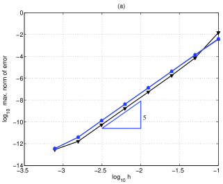
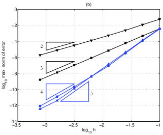
Figure 1: These plots show the numerical convergence of SIMEX-RK, part (a), and IMEX-RK, part (b) when applied to Eq. Eq. 25. The ordinate shows the $\log_{10}||\cdot||_{\infty}$ of the error between the reference exact solution of Eq. Eq. 25 at $t=1$ and the approximate solution with step-size $h$. The type of marker indicates the number of iterations of Newton’s method: the markers with triangle pointing down, square, circle, and triangle pointing up, are respectively matched to $M$ = 0, 1, 2, and 3 iterations. In part (a), the markers almost overlap: SIMEX-RK is fifth order for every $M$. In contrast, in part (b), the convergence rate depends on $M$. When $M=3$, IMEX-RK is clearly fifth order but when $M=2$ the numerical convergence rate approaches fourth order.

For the second example, we perform a numerical experiment to show that the filter cannot be changed from one stage to another within the same step (this second example could be called a counter example instead). In this experiment, the setting is the same used for Eq. (25) (shown in Fig. 1) the only exception is in Algorithm 3 which is replaced by a purposely bugged version: Between lines 5 and 13 of Algorithm 3, this bugged version computes $\eta_{rbd}={\cal F}^{Newt(2)}({\mathbf{r}})$ when $i$ is even and computes $\eta_{rbd}={\cal F}^{Newt(1)}({\mathbf{r}})$ when $i$ is odd. This means that either 1 or 2 iterations are being alternately used at each stage. The result of this numerical experiment (not shown graphically) is the following: the convergence rate of SIMEX-RK drops to third order instead of maintaining the fifth order shown in Fig. 1(a). In summary, one cannot omit the “if $i=2$” statement in line 5 of Algorithm 3 because this can cause an erroneous step whenever the number of iterations varies among stages within the same step.

6 Some stability regions for SIMEX-RK

In this section we explore time-step stability of the SIMEX-RK algorithm when applied to a stiff model PDE. For a SIMEX-RK method, the stability depends on the choice of the RK tableau, the choice of the proto-decomposition, and the choice of filter.

The scalar model equation $y^{\prime}=zy$, with $z\in\mathbb{C}$, is not a useful model for studying SIMEX’s stability because the influence of the filter is lost. Here, we extend the scalar model equation to an ODE system by considering the stability of the SIMEX method for an ODE system with the form

(26) $$\frac{d{\mathbf{y}}}{dt}=zA{\mathbf{y}},$$

where $z\in\mathbb{C}$ and $A$ is a matrix with at least one eigenvalue equal to $1$ and spectral radius equal to one, $\rho(A)=1$. A point $z\in\mathbb{C}$ belongs to the stability region $\Omega(A)$ when the numerical sequence ${\mathbf{y}}_{n}$ generated by the time-stepping method applied to Eq. Eq. 26 whit $h=1$ converges asymptotically to zero as $n\rightarrow+\infty$ for every unit-size initial condition. With this definition, the region defined by the scalar model equation is denoted by $\Omega(1)$.

The matrix $A$ in Eq. Eq. 26 should represent a typical application of interest. Here we address the stability of SIMEX-RK when the method of lines is applied to a spatial discretization of the equation

(27) $$\frac{\partial u}{\partial t}=-\lambda\Delta u$$

where $\lambda\in\mathbb{C}$ with $|\lambda|=1$, and where $u({\mathbf{x}},t)$ is defined in the domain ${\mathbf{x}}\in[0,\pi]^{2}$ with periodic boundaries. This model addresses both diffusive and dispersive effects of second order PDEs. We test the stability of SIMEX-RK by choosing the proto-decomposition with $-\lambda\Delta u$ in the implicit part and zero in the explicit part. In this way, the explicit part of the RBD holds the “leakage term” which is the residual term given in expression Eq. 15. Thus, the stability region is constrained by the stiffness present in this term.

Here, the Laplacian is discretized with standard second-order, five points, finite-difference stencil on a uniform grid. Let $N$ denote the number of discretization points along each edge of the domain and let $\delta x=\pi/N$ be the spacing between grid points. Denote the discretized Laplacian by $\Delta_{\delta x}$. We define the matrix $A_{N}$ according to $A_{N}=\sigma_{1}^{-1}\Delta_{\delta x}$ where $\sigma_{1}$ is the eigenvalue of $\Delta_{\delta x}$ with the largest module. We compute $\sigma_{1}$ numerically (a good analytical approximation is $\sigma_{1}\approx-8/\delta_{x}^{2}$). In numerical experiments we use $A=A_{N}$ in Eq. Eq. 26 with $N=50$.

An approximate stability region $\Omega(A_{N})$ is computed by placing a grid on the complex-plane and then computing if each $z$ on the grid belongs to $\Omega(A_{N})$ or not. To establish this for a given $z$, eight initial condition are randomly generated with unitary $l_{2}$ norm. Then, 30 time steps of Algorithm 2 (computed with $h=1$) are applied to each initial condition. The amplification factor for each initial condition is recorded. The maximum amplification factor over this eight initial conditions is stored as the numerical amplification factor.

Fig. 2 shows the stability region obtained numerically with the CNH tableau using both GMRES and Jacobi iterations as filters. Fig. 3 shows the stability for the ARK436 tableau with the same filters. These figures show a plot of the level curve of value 1 of the numerically computed amplification factor. In both figures the stability region increases as the number of iterations increase. The ARK436 tableau has more stages than CNH and it produces larger stability regions when using the same filter. In the case of GMRES iterations, the irregularity on the boundary of the stability region occurs because the initial condition strongly influences the sequence of Krylov subspace which appear along the time steps. Nevertheless, the bulk part of the interior of the stability region is not sensitive to the initial condition. Unlike GMRES iterations, Jacobi iterations produce stability regions with smooth boundaries.

When comparing the regions obtained with one GMRES iteration (continuous black line) and with seven Jacobi iterations (dashed red line), it is visible that these stability regions are similar in Fig. 2 but are different in Fig. 3. In Fig. 3, a larger region is obtained with Jacobi iterations. This shows that the choice of tableau and filter are interdependent in stability issues.

Figure 2: Complex plane showing the approximate stability regions $\Omega(A_{N})$ of the SIMEX-RK method, Algorithm 2, using the CNH tableau with both GMRES and Jacobi iterations as filters. The solid lines correspond to the regions obtained with 1, 2, 3, and 4 GMRES iterations without preconditioning. The stability region increases as the number of iterations increase. The two dashed lines correspond to Jacobi’s method with 1 iteration and 7 iterations.

Figure 3: Complex plane showing the approximate stability regions $\Omega(A_{N})$ of the SIMEX-RK method in Algorithm 2 using the ARK436 tableau with both GMRES and Jacobi iterations as filters. The solid lines represent the regions where the filter has 1 and 2 GMRES iterations. The dashed lines correspond to the filters that use Jacobi’s method with 1 iteration and 7 iterations.

7 Comparing SIMEX and IMEX on a stiff ODE

This section brings a numerical experiment where SIMEX and IMEX are compared in an ODE system obtained after the spatial discretization of an advection-diffusion-reaction equation in 2D. The spatial grid is moderately refined and parabolic stiffness is predominant. This example is adapted from [22] by adding an advection term.

The ODE system is derived from the spatial discretization of the PDE system

(28) $$\frac{\partial u}{\partial t}+{\mathbf{w}}\cdot\nabla u =1-4.4u+u^{2}v+0.6\Delta u+\psi_{u}$$

(29) $$\frac{\partial v}{\partial t}+{\mathbf{w}}\cdot\nabla v =1+3.4u-u^{2}v+0.6\Delta v+\psi_{v}$$

where $u(x_{1},x_{2},t)$ and $v(x_{1},x_{2},t)$ is defined in the spatial domain $[0,\pi]^{2}$ with periodic boundaries and where ${\mathbf{w}}=(1/2,\sqrt{3}/2)$ is a constant vector. The functions $\psi_{u}$ and $\psi_{v}$ are chosen consistent with the exact solution $u_{exact}(t,x_{1},x_{2})=\exp(-\sin(t-4x_{1}-2x_{2}))$ and $v_{exact}(t,x_{1},x_{2})=\exp(\cos(t-2x_{1}-6x_{2}))$. All partial derivatives are discretized with fourth-order finite-difference formulas which use stencils with five points in each Cartesian direction. In this way, the discretized Laplacian has a 9-point stencil with a cross shape. The number of discretization points along each Cartesian direction is $N=2^{7}$; the spatial grid is uniform with $\delta x$ spacing between grid points. This leads to an ODE system with $2^{15}$ degrees of freedom.

The proto-decomposition places the discretized diffusion term in the implicit part ${\mathbf{g}}({\mathbf{y}})$ and the remaining terms in the explicit part ${\mathbf{f}}({\mathbf{y}},t)$. Time integration is carried out in $t\in[0,\pi]$. In numerical experiments, the step size parameter is chosen as $h_{j}=2^{-j}/10$, for $j=0,1,\cdots,8$. The reference exact solution for the ODE is obtained from the “ode45” routine with $AbsTol$ and $RelTol$ equal to $10^{-14}$.

SOR iterations are used for the implicit equation $(I-(0.6\gamma h_{j}/\delta x^{2})M_{\delta x})\eta={\mathbf{r}}$ where $0.6\delta x^{-2}M_{\delta x}$ is the matrix resulting from the discretization of the diffusion operator. The stopping criterion relies on the relative reduction of the residual which means the iterations stop when

$$||(I-(0.6\gamma h/\delta x^{2})M_{\delta x})\eta^{(j)}-{\mathbf{r}}||_{\infty}\leq\zeta||(I-(0.6\gamma h/\delta x^{2})M_{\delta x})\eta^{(0)}-{\mathbf{r}}||_{\infty}$$

where $\zeta$ is the relative reduction parameter and $\eta^{(0)}={\mathbf{r}}$ is the initial guess.

The stopping criterion for IMEX’s solver is chosen to be the same as the stabilization criterion in Algorithm 3. In numerical experiments, $\zeta$ varies as $\zeta_{m}=2^{-m}$ for $m=0,1,\cdots,10$; and it remains constant throughout the steps of each time integration. The case $\zeta_{0}=1$ is included here in order to allow SIMEX-RK to use the default filter, i.e., no SOR iterations are performed. In all experiments, the relaxation parameter for SOR is $\omega=1.2$.

All pairs of parameters $(h_{j},\zeta_{m})$ are tested experimentally. Fig. 4 shows a scatter plot of the resulting value of the error (measured by the root mean square difference to the reference solution) and CPU time (measured in seconds of a i5-7200U Intel processor) for four different time-integration methods: SIMEX, IMEX, both using the ARK436 tableau; the classic 4th order RK method, and the 3rd order Heun’s method. Because these last two methods are not stable for the time-grid $h_{8}$, there is only one data point shown for each of them where the data is obtained with the time-grid $h_{9}=2^{-9}/10$. This figure also shows a line connecting the Pareto optimal data points of each method where a Pareto optimal point is one for which there is no other data point of the same method with both a lower error and a lower CPU time. Most of SIMEX’s data points are below IMEX’s Pareto optimal points. One of SIMEX’s data points is close to the RK4 method, this point is obtained with the default filer and time-grid $h_{8}$.

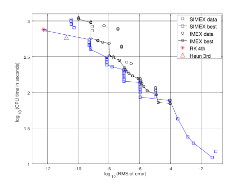
Figure 4: Each data point marks the $\log_{10}$ of the r.m.s. error versus the $\log_{10}$ of CPU time (in seconds) obtained experimentally for each pair of parameters $(h_{j},\zeta_{m})$ and for each of four methods: SIMEX-RK, IMEX-RK (both using the ARK436 tableau), the classical 4th order RK, and the 3rd order Heun’s method. For the last two, only the $h_{j}$ parameter is relevant. Only the data that resulted in a numerically stable time integration is shown. The explicit methods are stable only for $h_{9}$. Solid lines connect the Pareto optimal points of each method.

In order to examine SIMEX’s efficiency, Table 1 shows the data from Fig. 4 where $h$ is fixed equal to $h_{7}$ and $\zeta$ changes form $\zeta_{2}$ to $\zeta_{10}$ (the other values of $\zeta_{m}$ are omitted due to instabilities which occurred simultaneously in both methods). This table shows that, given the time step $h_{7}$, the SIMEX method yields a precise solution almost as soon as $\zeta$ is small enough to stabilize it. In contrast, the IMEX method requires a smaller value of $\zeta$ in order to improve the precision of the solver. Thus, for the IMEX method, there is a significant gap between the value of $\zeta$ needed for a stable output and the value of $\zeta$ needed for an accurate output. By avoiding this precision gap, the SIMEX method gains some computational time.

$\zeta$	SIMEX error	IMEX error	SIMEX CPU time	IMEX CPU time
$\zeta_{2}$	6.7163e-10	6.7375e-08	403.06	428.31
$\zeta_{3}$	6.7163e-10	6.7374e-08	399.44	434.63
$\zeta_{4}$	6.7163e-10	6.7374e-08	415.26	444.09
$\zeta_{5}$	5.2848e-10	1.0279e-08	452.63	485.38
$\zeta_{6}$	5.2848e-10	1.0279e-08	454.56	484.94
$\zeta_{7}$	5.2848e-10	3.967e-09	466.6	503.53
$\zeta_{8}$	5.1764e-10	1.9183e-09	498.41	529.99
$\zeta_{9}$	5.1764e-10	1.9183e-09	503.07	534.61
$\zeta_{10}$	5.1566e-10	6.786e-10	549.28	574.62

Table 1: This table shows the error and CPU time for both SIMEX-RK and IMEX-RK methods obtained with different values of $\zeta_{m}$ while $h$ remains fixed equal to $h_{7}=7.8125\times 10^{-4}$. SIMEX’s error is small already for $\zeta_{2}$ ($\zeta_{2}=0.25$). In contrast, IMEX requires the stopping criteria to use $\zeta_{10}$ in order to reach the same error.

8 Conclusion

In this article the residual balanced decomposition (RBD) for IMEX methods is introduced. Given a proto-decomposition (implicit and explicit parts ${\mathbf{g}}$ and ${\mathbf{f}}$) and given a filter (which is a map following Definition 3.1), RBD provides a new within-step decomposition where the implicit equation is solved exactly without additional computational work. This remarkable property allows great freedom for exploring the numerical properties of the resulting algorithm. The decomposition itself is rather abstract, Eqs. Eqs. 10 and 11, but the computational steps for its evaluation are straightforward, Eq. Eq. 13. The implementation effort is negligible. Here, RBD is used with IMEX-RK methods that have ESDIRK implicit schemes, the resulting method is the SIMEX-RK method in Algorithm 2. The proof of convergence of Algorithm 2 is given in Section 4.

By defining a suitable ODE system, stability regions can be drawn in the complex plane in order to observe the stability of the SIMEX method. The stability region can vary significantly depending on the combination of tableau and filter being used. The size of the stability region clearly depends on the computational effort placed in the filter.

The goal of the filter is to provide time-step stability because SIMEX can maintain an accurate time integration even if the implicit equation Eq. Eq. 8 is not solved accurately. This property leads to the computational improvement observed in Section 7. One way to construct a filter is to fix the number of iterations of an iterative solver applied to the implicit equation. Another way is to stop the iterations after the residual has been reduced by a certain amount. In any case, Algorithm 3 brings the necessary changes to Algorithm 2 in order to allow a within-step filter selection. As explained in Section 5, the iterative process in Algorithm 3 can be made very similar to Algorithm 1. For these reasons, and for the additional flexibility, the SIMEX method seems to be preferable to the IMEX method.

References

- [1] X. Antoine, C. Besse, and V. Rispoli, High-order IMEX-spectral schemes for computing the dynamics of systems of nonlinear Schrodinger/Gross-Pitaevskii equations, J. Comp. Phys., 327 (2016), pp. 252–269.
- [2] U. M. Ascher, S. J. Ruuth, and R. J. Spiteri, Implicit-explicit Runge-Kutta methods for time-dependent partial differential equations, Applied Numerical Mathematics, 25 (1997), pp. 151–167.
- [3] U. M. Ascher, S. J. Ruuth, and B. T. R. Wetton, Implicit-explicit methods for time-dependent partial differential equations, SIAM J. Numer. Anal., 32 (1995), pp. 797–823.
- [4] G. Bispen, M. Lukáčová-Medvid’ová, and L. Yelash, Asymptotic preserving IMEX finite volume schemes for low Mach number Euler equations with gravitation, Journal of Computational Physics, 335 (2017), pp. 222–248.
- [5] S. Blaise, J. Lambrechts, and E. Deleersnijder, A stabilization for three-dimensional discontinuous Galerkin discretizations applied to nonhydrostatic atmospheric simulations, International Journal for Numerical Methods in Fluids, 81 (2016), pp. 558–585.
- [6] S. Boscarino, L. Pareschi, and G. Russo, Implicit-explicit Runge-Kutta schemes for hyperbolic systems and kinetic equations in the diffusion limit, SIAM J. Sci. Comput., 35 (2013), pp. A22–A51.
- [7] S. Boscarino, L. Pareschi, and G. Russo, A unified IMEX Runge–Kutta approach for hyperbolic systems with multiscale relaxation, SIAM Journal on Numerical Analysis, 55 (2017), pp. 2085–2109.
- [8] M. Braś, A. Cardone, Z. Jackiewicz, and P. Pierzchała, Error propagation for implicit–explicit general linear methods, Applied Numerical Mathematics, 131 (2018), pp. 207–231.
- [9] J. H. Chaudhry, D. Estep, V. Ginting, J. N. Shadid, and S. Tavener, A posteriori error analysis of IMEX multi-step time integration methods for advection-diffusion-reaction equations, Computer Methods in Applied Mechanics and Engineering, 285 (2015), pp. 730–751.
- [10] C. Colavolpe, F. Voitus, and P. Bénard, RK-IMEX HEVI schemes for fully compressible atmospheric models with advection: analyses and numerical testing, Quarterly Journal of the Royal Meteorological Society, 143 (2017), pp. 1336–1350.
- [11] G. J. Cooper and A. Sayfy, Additive methods for the numerical solution of ordinary differential equations, Math. Comp., 35 (1980), pp. 1159–1172.
- [12] G. J. Cooper and A. Sayfy, Addtive Runge-Kutta methods for stiff ordinary differential equations, Math. Comp., 40 (1983), pp. 207–218.
- [13] M. Crouzeix, Une méthode multipas implicite-explicite pour l’approximation des équations d’evolution paraboliques, Numer. Math., 35 (1980), pp. 257–276.
- [14] D. R. Durran and P. N. Blossey, Implicit-explicit multistep methods for fast-wave-slow-wave problems, Monthly Weather Review, 140 (2012), pp. 1307–1325.
- [15] B. Froehle and P.-O. Persson, A high-order discontinuous Galerkin method for fluid-structure interaction with efficient implicit-explicit time stepping, J. Comp. Phys., 272 (2014), pp. 455–470.
- [16] F. Garcia, L. Bonaventura, M. Net, and J. Sánchez, Exponential versus IMEX high-order time integrators for thermal convection in rotating spherical shells, J. Comp. Phys., 264 (2014), pp. 41––54.
- [17] F. Garcia, M. Net, B. García-Archilla, and J. Sánchez, A comparison of high-order time integrators for thermal convection in rotating spherical shells, J. Comp. Phys., 229 (2010), pp. 7997––8010.
- [18] D. J. Gardner, J. E. Guerra, F. P. Hamon, D. R. Reynolds, P. A. Ullrich, and C. S. Woodward, Implicit–explicit (IMEX) Runge–Kutta methods for non-hydrostatic atmospheric models, Geoscientific Model Development, 11 (2018), pp. 1497–1515.
- [19] D. Ghosh and E. Constantinescu, Semi-implicit time integration of atmospheric flows with characteristic-based flux partitioning, SIAM Journal on Scientific Computing (SISC), 38 (2016), pp. A1848–A1875, doi:10.1137/15M1044369.
- [20] D. Ghosh, M. A. Dorf, M. R. Dorr, and J. A. Hittinger, Kinetic simulation of collisional magnetized plasmas with semi-implicit time integration, Journal of Scientific Computing, 77 (2018), pp. 819–849.
- [21] E. Hairer, S. Nørsett, and G. Wanner, Solving Ordinary Differential Equations I: Nonstiff Problems, Springer Series in Computational Mathematics, Springer Berlin Heidelberg, 2008.
- [22] E. Hairer and G. Wanner, Solving Ordinary Differential Equations II: Stiff and Differential - Algebraic Problems, Springer Series in Computational Mathematics, Springer Berlin Heidelberg, 2013.
- [23] I. Higueras and T. Roldán, Construction of additive semi-implicit Runge–Kutta methods with low-storage requirements, J. Sci. Comput., 67 (2016), pp. 1019–1042.
- [24] E. Hofer, A partially implicit method for large stiff systems of ODEs with only few equations introducing small time-constants, SIAM Journal on Numerical Analysis, 13 (1976), pp. 645–663.
- [25] D. Z. Huang, P.-O. Persson, and M. J. Zahr, High-order, linearly stable, partitioned solvers for general multiphysics problems based on implicit–explicit Runge–Kutta schemes, Computer Methods in Applied Mechanics and Engineering, 346 (2019), pp. 674–706.
- [26] Z. Jackiewicz and H. Mittelmann, Construction of IMEX DIMSIMs of high order and stage order, Applied Numerical Mathematics, 121 (2017), pp. 234–248.
- [27] A. Kanevsky, M. H. Carpenter, D. Gottlieb, and J. S. Hesthaven, Application of implicit-explicit high order Runge-Kutta methods to discontinuous-Galekin schemes, J. Comp. Physics, 225 (2007), pp. 1753–1781.
- [28] V. Kazemi-Kamyab, A. van Zuijlen, and H. Bijl, Analysis and application of high order implicit Runge-Kutta schemes for unsteady conjugate heat transfer: A strongly-coupled approach, J. Comput. Physics, 272 (2014), pp. 471–486.
- [29] C. A. Kennedy and M. H. Carpenter, Additive Runge-Kutta schemes for convection-diffusion-reaction equations, Technical report NASA/TM-2001-211038, (2001).
- [30] C. A. Kennedy and M. H. Carpenter, Diagonally implicit Runge-Kutta methods for ordinary differential equations. A review, Technical report NASA/TM-2016-219173, (2016).
- [31] C. A. Kennedy and M. H. Carpenter, Higher-order additive Runge–Kutta schemes for ordinary differential equations, Applied Numerical Mathematics, 136 (2019), pp. 183–205.
- [32] C. A. Kennedy, M. H. Carpenter, and R. M. Lewis, Additive Runge-Kutta schemes for convection-diffusion-reaction equations, Appl. Numer. Math., 44 (2003), pp. 139–181.
- [33] P. Mati, M. A. Calkins, and K. Julien, A computationally efficient spectral method for modeling core dynamics, Geochemeistry, Geophysics, Geosystems, 17 (2016), pp. 3031–3053.
- [34] P.-O. Persson, High-order LES simulations using implicit-explicit Runge-Kutta schemes, in 49th AIAA Aerospace Sciences Meeting including the New Horizons Forum and Aerospace Exposition, AIAA 2011-684, (2011), doi:10.2514/6.2011-684.
- [35] M. Restelli and F. X. Giraldo, A conservative discontinuous Galerkin semi-implicit formulation for the Navier-Stokes equations in nonhydrostatic mesoscale modeling, SIAM J. Sci. Comput., 31 (2009), pp. 2231–2257.
- [36] D. Ruprecht and R. Speck, Spectral deferred corrections with fast-wave slow-wave splitting, SIAM J. Sci. Comput., 38 (2016), pp. A2535–A2557.
- [37] Y. Saad, Iterative Methods for Sparse Linear Systems: Second Edition, Other Titles in Applied Mathematics, Society for Industrial and Applied Mathematics, 2003.
- [38] M. P. Ueckermann and P. F. J. Lermusiaux, Hybridizable discontinuous Galerkin projection methods for Navier-Stokes and Boussinesq equations, J. Comp. Physics, 306 (2016), pp. 390–421.
- [39] A. H. van Zuijlen and H. Bijl, Implicit and explicit higher order time integration schemes for structural dynamics and fluid-structure interaction computations, SIAM J. Sci. Comput., 38 (2016), pp. A1430–A1453.
- [40] H. Wang, C.-W. Shu, and Q. Zhang, Stability and error estimates of local discontinuous Galerkin methods with implicit-explicit time-marching for advection-diffusion problems, SIAM J. Numer. Anal., 53 (2015), pp. 206–227.
- [41] H. Wang, C.-W. Shu, and Q. Zhang, Stability analysis and error estimates of local discontinuous Galerkin methods with implicit-explicit time-marching for nonlinear convection-diffusion problems, Applied Mathematics and Computation, 272 (2016), pp. 237–258.
- [42] H. Weller, S.-J. Lock, and N. Wood, Runge-Kutta IMEX schemes for the horizontally explicit/vertically implicit (HEVI) solution of wave equations, J. Comp. Physics, 252 (2013), pp. 365–381.
- [43] A. J. Wright and I. Hawke, Resistive and multi-fluid RMHD on graphics processing units, The Astrophysical Journal Supplement Series, 240 (2019), p. 8.
- [44] H. Zhang, A. Sandu, and S. Blaise, High order implicit-explicit general linear methods with optimized stability regions, SIAM J. Sci. Comput., 38 (2016), pp. A1430–A1453.