Ultra-luminous X-ray sources and neutron-star–black-hole mergers from very massive close binaries at low metallicity

The detection of gravitational waves from the binary black hole (BH) merger GW150914 may enlighten our understanding of ultra-luminous X-ray sources (ULXs), as BHs of masses $>30M_{\odot}$ can reach luminosities $>4\times 10^{39}\leavevmode\nobreak\ {\rm erg\leavevmode\nobreak\ s^{-1}}$ without exceeding their Eddington luminosities. It is then important to study variations of evolutionary channels for merging BHs, which might instead form accreting BHs and become ULXs. It was recently shown that very massive binaries with mass ratios close to unity and tight orbits can undergo efficient rotational mixing and evolve chemically homogeneously, resulting in a compact BH binary. We study similar systems by computing $\sim 120\,000$ detailed binary models with the MESA code covering a wide range of masses, orbital periods, mass ratios and metallicities. For initial mass ratios $q\equiv M_{2}/M_{1}\simeq 0.1-0.4$, primaries with masses above $40M_{\odot}$ can evolve chemically homogeneously, remaining compact and forming a BH without experiencing Roche-lobe overflow. The secondary then expands and transfers mass to the BH, initiating a ULX phase. At a given metallicity this channel is expected to produce the most massive accreting stellar BHs and the brightest ULXs. We predict that $\sim 1$ out of $10^{4}$ massive stars evolves this way, and that in the local universe $0.13$ ULXs per $M_{\odot}\leavevmode\nobreak\ \rm yr^{-1}$ of star-formation rate are observable, with a strong preference for low-metallicities. An additional channel is still required to explain the less luminous ULXs and the full population of high-mass X-ray binaries. At metallicities $\log Z>-3$, BH masses in ULXs are limited to $60M_{\odot}$ due to the occurrence of pair-instability supernovae which leave no remnant, resulting in an X-ray luminosity cut-off for accreting BHs. At lower metallicities, very massive stars can avoid exploding as pair-instability supernovae and instead form BHs with masses above $130M_{\odot}$, producing a gap in the ULX luminosity distribution. After the ULX phase, neutron-star-BH binaries that merge in less than a Hubble time are produced with a low formation rate $<0.2\leavevmode\nobreak\ \rm Gpc^{-3}yr^{-1}$. We expect that upcoming X-ray observatories will test these predictions, which together with additional gravitational wave detections will provide strict constraints on the origin of the most massive BHs that can be produced by stars.

1 Introduction

One of the most puzzling discoveries made by the Einstein Observatory are the off-nucleus X-ray point sources with luminosities above $10^{39}\leavevmode\nobreak\ {\rm erg\leavevmode\nobreak\ s^{-1}}$ (Long & van Speybroeck, 1983), which owing to their extreme luminosities were termed ultra-luminous X-ray sources (ULXs). Compared to the typical properties of high-mass X-ray binaries (HMXBs), such high luminosities are difficult to explain in terms of accreting compact objects, as the Eddington limit for neutron stars ($\sim 10^{38}{\rm erg\leavevmode\nobreak\ s^{-1}}$, hereafter NS) and stellar mass black holes ($\sim 2\times 10^{39}{\rm erg\leavevmode\nobreak\ s^{-1}}$ for a $10M_{\odot}$ black hole, hereafter BH) is well below the luminosities of some of the observed sources. One possibility to explain these high luminosities is to consider the existence of a population of intermediate-mass BHs (IMBHs), with masses between $\sim 10^{2}-10^{5}M_{\odot}$, possibly arising from the collapse of primordial stars (eg. Madau & Rees 2001) or formed in dense globular clusters (eg. Miller & Hamilton 2002).

As the Chandra X-ray Observatory and other facilities opened up the possibility of studying populations of X-ray point sources in galaxies down to much lower luminosities, Grimm et al. (2003) showed that ULXs generally correspond to the tail of the HMXB population, and their number is strongly correlated with star-formation rate (SFR). Swartz et al. (2011) estimated a typical number of $\sim 2$ ULXs per $M_{\odot}\leavevmode\nobreak\ {\rm yr^{-1}}$ of SFR for a local sample of galaxies, while Luangtip et al. (2015) observed that there is a scarcity of ULXs in luminous infrared galaxies, with an estimated number of $0.2$ ULXs per $M_{\odot}\leavevmode\nobreak\ {\rm yr^{-1}}$ of SFR. All of this points towards both a stellar origin for ULXs and possibly a strong metallicity dependence, which disfavors the IMBH scenario. Using a sample of 64 galaxies at various metallicities down to $\log Z\,{\sim}\,{-}3$, Mapelli et al. (2010) found that the number of ULXs per $M_{\odot}\leavevmode\nobreak\ {\rm yr^{-1}}$ of SFR scales with metallicity as $Z^{-0.55\pm 0.23}$ (see also Prestwich et al. 2013). Although this appears to rule out IMBHs as the central engines of most ULXs, there remain a handful of particularly bright sources (in excess of $3\times 10^{41}\leavevmode\nobreak\ {\rm erg\leavevmode\nobreak\ s^{-1}}$) which appear to form an independent population (Sutton et al., 2012; Swartz et al., 2011). The term hyper-luminous-X-ray-source has been coined for these objects, with ESO243-49 HLX-1 being the best current candidate for an IMBH (Farrell et al., 2009). However, some of these have been confirmed to be background AGN (Sutton et al., 2015), reducing the number of known objects of this class.

If ULXs have a stellar origin, there are various potential explanations for their high luminosities. For instance, beaming of the radiation emitted would imply that the actual full-sky luminosity of these sources is much lower, so that ULXs could consist of BHs with masses below $10M_{\odot}$ accreting at or below the Eddington rate. This could be a purely geometrical effect (King et al., 2001) or the result of relativistic beaming (Körding et al., 2002), but measurements from ionization nebulae around some ULXs appear to confirm the isotropic estimate of their luminosities (Pakull & Mirioni, 2003). On the other hand, Begelman (2002) and Ruszkowski & Begelman (2003) proposed that the photon-bubble instability, which acts on radiation-dominated accretion disks and produces clumping, would cause photons to be radiated away through low density regions allowing for accretion rates up to 10 times the Eddington rate. The presence of a corona supported by strong magnetic fields could also help to counter the radiation pressure and allow super-Eddington accretion (Socrates & Davis, 2006).

A clear case of super-Eddington accretion is the recently observed NS-ULX (Bachetti et al., 2014), for which accretion rates above a hundred times the Eddington rate are required to explain its luminosity in excess of $10^{40}\leavevmode\nobreak\ {\rm erg\leavevmode\nobreak\ s^{-1}}$. The flux observed from this object has both a pulsed component with a period of $1.37$ days, and a non-pulsed component, so beaming alone appears insufficient to explain its nature.Very recently, two more ULXs powered by NSs have been discovered (Israel et al., 2016, 2017), and some argue that a significant fraction of ULXs could contain a NS accretor (King & Lasota, 2016). The very high luminosities of these accreting NSs do not necessarily imply that accreting BHs can also radiate well above their Eddington luminosities, since the accretion flows around NSs and BHs should differ substantially.

It should also be considered that, although Galactic BHs are limited to masses below $\sim 20M_{\odot}$ due to strong wind mass loss (Fryer & Kalogera, 2001; Spera et al., 2015; Sukhbold et al., 2016), in lower metallicity environments BH masses could reach up to $45M_{\odot}$ (Heger & Woosley, 2002; Belczynski et al., 2016a), with the mass being limited by the effects of pair-instability supernovae (PISNe) and pulsational-pair-instability supernovae (PPISNe). Such massive BHs can easily account for the luminosity of ULXs, requiring accretion rates only slightly above the Eddington limit to explain some of the brightest sources (Zampieri & Roberts, 2009). For massive enough progenitors, it is expected that PISNe can be avoided, resulting in BHs with masses above $\sim 130M_{\odot}$ and possibly causing a gap in the BH mass distribution (Heger & Woosley, 2002). However, for single stars this requires extremely high zero-age main-sequence masses and low metallicity.

1.1 Formation channels for ULXs and merging binary BHs

The commonly assumed model for ULX formation involves the occurrence of a CE phase in an initially very wide binary (Rappaport et al., 2005). In these models, the envelope of the primary is stripped in a common-envelope (CE) phase, which significantly reduces the orbital period. The primary then collapses to a BH, and when the secondary expands and initiates Roche-lobe overflow (RLOF) the system becomes an active X-ray source. Whether a standard HMXB or a ULX is produced depends on the mass of the BH formed, providing a simple explanation for the continuous luminosity distribution function from HMXBs to ULXs, although accretion rates $\sim 10$ times Eddington are still required to explain the brightest sources. A different possibility is the formation of ULXs containing a BH through dynamical interactions in star clusters (Mapelli & Zampieri, 2014; MacLeod et al., 2016), which could potentially produce more massive BHs at a given metallicity, as the progenitor of the BH can evolve as a single star and avoid envelope stripping in a binary.

The first observation from the twin LIGO detectors in Hanford and Livingston of gravitational waves (GWs) from the inspiral and merger of two $\sim 30M_{\odot}$ BHs (GW150914, Abbott et al. 2016a) plays a particularly important role in our understanding of ULX progenitor systems. Any formation channel that can produce BHs above $30M_{\odot}$ is likely to be related to the formation of ULXs, as the occurrence of RLOF would easily result in very high luminosities. There are three main channels that can explain the origin of GW150914, the classical field scenario involving CE evolution (Tutukov & Yungelson, 1993; Belczynski et al., 2016b; Kruckow et al., 2016), the dynamical scenario in globular and nuclear clusters (Portegies Zwart & McMillan, 2000; Rodriguez et al., 2016), and the chemically homogeneous evolution (CHE) channel for field binaries (Mandel & de Mink, 2016; Marchant et al., 2016; de Mink & Mandel, 2016) which we illustrate in Figure 1. The ocurrence of CHE in binaries was first proposed by de Mink et al. (2009) and has only recently been studied in more detail (Song et al., 2016; Mandel & de Mink, 2016; Marchant et al., 2016; de Mink & Mandel, 2016).

Studying variations of channels for the production of GW sources can then provide insight into the origin of ULXs. For instance, in the CE scenario for merging binary BHs the primary is stripped through stable mass transfer, collapses into a BH, and a CE phase happens when the secondary expands to become a giant. However, considering the possibility that stable mass transfer develops instead of a CE, Pavlovskii et al. (2017) showed that systems similar to the progenitor of GW150914 could instead form a ULX with a red supergiant as the donor. Recognizing different branches of binary BH formation channels resulting not only in GW emission, but also in electromagnetic waves, will play a fundamental role in constraining different formation scenarios of GW sources.

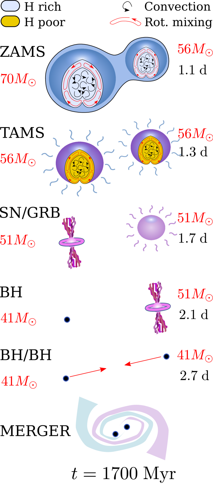
Figure 1: The CHE channel for the formation of double-BHs, including the occurrence of an overcontact phase as in Marchant et al. (2016). Numbers correspond to a system with $Z=Z_{\odot}/50$, initial masses $M_{1}=70M_{\odot}$ and $M_{2}=56M_{\odot}$, and a very short initial period at the zero-age main sequence (ZAMS). This system evolves early on into a contact configuration, where mass is transferred back and forth until a mass ratio of unity is achieved. Efficient rotational mixing distributes the helium rich material from the core throughout the entire envelope, resulting in an almost pure helium star at the terminal-age main sequence (TAMS). Depending on the final masses of each component, the system may then proceed to form a compact BH binary that can merge within a Hubble time, or explode as a PISNe. The models from Marchant et al. (2016) had an error in the computation of spin-orbit coupling which resulted in slightly wider orbits. We have corrected for this, so the values differ slightly from those in Marchant et al. (2016). We have also verified that the conclusions of that work remain valid despite this issue.

In this paper we consider an alternative channel for the formation of ULXs, which is a variation of the CHE channel for merging binary BHs. In this scenario, the initial configuration is a very massive binary with a period $\sim 1$ day and a mass ratio far from unity. It is then expected that only the primary star undergoes efficient rotational mixing (as proposed by de Mink et al. 2009), avoiding a binary interaction before forming a massive BH. The less massive component in such a system will evolve normally, eventually undergoing RLOF and initiating mass transfer. As the resulting BH will usually be more massive than the secondary, this results in a long-lived ULX phase, with mass transfer proceeding on a nuclear timescale. Such a channel of evolution is strongly related to the formation of merging double BHs, PISNe and LGRBs, and could be the source of the most luminous X-ray sources of stellar origin that can be formed under any given conditions. In Section 2 we describe the setup of our stellar evolution models, and present our model for ULX formation in Section 3. We then discuss the consequences of this channel for the luminosity distribution of ULXs in Section 4, and their orbital parameters in Section 5. In Section 6 we discuss the formation of NS-BH and BH-BH binaries after a ULX phase, and the possibility to form systems compact enough to merge in less than a Hubble time. We give our concluding remarks in Section 7.

2 Methods

We extend the models computed by Marchant et al. (2016) to lower initial mass ratios to study the possibility of the primary evolving chemically homogeneously and forming a BH, while the secondary evolves on a much longer timescale, avoiding early interaction. Our tool of choice for stellar modeling is version 8845 of the MESA code (Paxton et al., 2011, 2013, 2015) . We model about a $120\,000$ binary systems for metallicities in the range $\log\leavevmode\nobreak\ Z=-2$ to $-6$ in steps of $0.5$ dex, primary masses between $\log M_{1}/M_{\odot}=1.5-2.5$ ($30M_{\odot}-300M_{\odot}$) in steps of $0.05$ dex, mass ratios $q=M_{2}/M_{1}=0.05-0.6$ (which results in a range of secondary masses between $1.5M_{\odot}-180M_{\odot}$) in steps of $0.05$ and initial orbital periods between $0.5$ and $3$ days, in steps of $0.05$ days. At higher mass ratios we expect the formation of binary-BHs, as discussed in detail by Marchant et al. (2016).

2.1 Stellar evolution

For a given metallicity, the initial helium mass fraction is determined by assuming that it linearly increases with metallicity from the primordial value $Y=0.2477$ (Peimbert et al., 2007) at $Z=0$ to $Y=0.28$ at $Z=Z_{\odot}$. The value of the solar metallicity is taken as $Z_{\odot}=0.017$ (Grevesse et al., 1996).

We use the Ledoux criterion for convection, which we model using mixing-length theory (Böhm-Vitense, 1958) with a mixing length parameter $\alpha=1.5$. In regions that are stable according to the Ledoux criterion, but unstable according to the Schwarzschild criterion, we include semiconvective mixing as in Langer et al. (1983) with an efficiency parameter $\alpha_{\rm sc}=1$. Opacities are computed using CO-enhanced tables from the OPAL project (Iglesias & Rogers, 1996) with solar scaled abundances from Grevesse et al. (1996). As we do not need to follow the detailed nucleosynthetic evolution of our models, we use the simple nuclear networks basic.net, co_burn.net and approx21.net that are provided with MESA and are switched during runtime as needed to account for the later burning phases.

Stellar winds are implemented as in Brott et al. (2011), with mass loss for hot hydrogen-rich stars modeled as in Vink et al. (2001). Between a surface hydrogen composition of $X=0.7$ to $0.4$ we interpolate between the Vink rate and a tenth of the mass loss rate for hydrogen-poor stars of Hamann et al. (1995). For temperatures below that of the bi-stability jump, the rate is taken as the maximum between the Vink rate and that of Nieuwenhuijzen & de Jager (1990), though in practice the stars we model remain blue over most of their lifetimes, so this plays a negligible role. We scale the strength of stellar winds by a factor $(Z/Z_{\odot})^{0.85}$, extending the metallicity dependence predicted by Vink et al. (2001) for O/B stars to hydrogen-poor Wolf-Rayet and cool stars. Note that the metallicity dependence of winds is constrained by observations of massive stars in the Galaxy, the LMC and the SMC (Mokiem et al., 2007), the latter of which has a metallicity of about $0.2\,Z_{\odot}$. Any model at lower metallicities is neccesarily extrapolating these results. Measurements of mass loss at lower metallicities have been reported by Tramper et al. (2011), but are currently under dispute (Bouret et al., 2015).

Rotational mixing and angular momentum transport are treated as diffusive processes following Heger & Langer (2000), including the effects of Eddington-Sweet circulations, the Goldreich-Schubert-Fricke instability, and secular and dynamical shear, with an efficiency parameter $f_{c}=1/30$ (Chaboyer & Zahn, 1992), and a sensitivity to composition gradients parametrized by $f_{\mu}=0.1$ (Yoon et al., 2006). We also include transport of angular momentum due to the Spruit-Tayler dynamo (Spruit, 2002) following the implementation by Petrovic et al. (2005). The effect of centrifugal forces is modeled as in Endal & Sofia (1976). For the primary star, if central and surface helium mass fractions differ by more than $0.2$, we consider the system not to be homogeneously evolving and terminate the simulation.

2.2 Binary evolution

Both components in the binary are assumed to be tidally locked at the ZAMS, although for the lowest mast ratios and shortest orbital periods the Darwin instability (Darwin, 1879) could make the formation of such systems impossible. To account for this, we consider the minimum orbital separation $a_{\rm Darwin}=\sqrt{3(I_{1}+I_{2})/\mu}$ below which a binary would become unstable, where $I_{1}$ and $I_{2}$ are the moments of inertia of both components and $\mu$ is the reduced mass. Systems that have an initial orbital separation below $a_{\rm Darwin}$ are ignored in our analysis. Our models do not include the impact of tidal deformation on stellar structure, but account for tidal synchronization following Hurley et al. (2002) and Detmers et al. (2008), which follow the model for dynamical tides with radiative damping of Zahn (1975, 1977). The angular momentum deposited into each component is distributed throughout the entire star, as described in Paxton et al. (2015).

The evolution of orbital angular momentum considers the effects of mass loss, gravitational wave radiation and spin-orbit coupling, as described in Paxton et al. (2015). In particular, changes due to mass loss are computed by assuming that winds carry the specific orbital angular momentum corresponding to each component.

For these low mass ratios and short orbital periods we expect systems to quickly evolve to an overcontact configuration and a merger if the primary experiences RLOF. CE ejection is unlikely in this case due to the short orbital period and the strongly bound envelope. If the primary undergoes CHE, but the secondary expands and initiates mass transfer before BH formation, the orbit is expected to widen as mass is transferred from the less massive to the more massive star. This slows down the rotation of the primary as it remains tidally locked. At the same time, the primary accretes hydrogen-rich material at its surface. These two effects lead to the interruption of CHE. Because of this, we terminate our simulations if there is mass transfer from any component before BH formation.

After BH formation, if the secondary does not evolve chemically homogeneously, it will eventually expand and undergo RLOF. Low-mass helium stars are expected to undergo an additional phase of mass transfer after helium depletion, which is called Case ABB or BB depending on whether the first mass-transfer event occurred before or after core-hydrogen depletion (Delgado & Thomas, 1981; Dewi et al., 2002). To study the possibility of forming merging BH-NS or BH-BH systems after interaction, we need to consider this additional phase of mass transfer, as due to the large mass ratios involved (the primary is expected to become a BH of more than $20M_{\odot}$), it can result in extreme orbital widening. To take this into account, we consider the evolution of the secondary star until core carbon depletion, or until mass transfer reaches hydrogen depleted regions. In case the latter happens, the orbit should widen significantly making the system irrelevant as a source of GWs.

2.3 BH and NS formation

If the primary star evolves to helium depletion, with a final mass outside the range $60-130M_{\odot}$, we assume it collapses directly to a BH without losing mass or receiving a kick, while inside that range we assume the star explodes as a PISN leaving no remnant (Heger & Woosley, 2002). The initial spin of the BH is computed as $a_{0}=Jc/M^{2}G$, meaning that we assume all the spin angular momentum $J$ contained in the star previous to collapse is retained. Note that this ignores possible mass loss due to PPISNe or LGRBs. PPISNe are expected to result in strong mass loss for helium stars with final masses above $\sim 40M_{\odot}$, and to limit the remnant mass to $\sim 47M_{\odot}$ (Woosley, 2016). Taking into account this effect would produce a reduction of $\sim 25\%$ in the maximum luminosity we predict from sources below the PISN gap. This is much smaller than the variations coming from uncertainties in the accretion rates. LGRBs are also expected to occur through the collapsar scenario (Woosley, 1993) when the pre-collapse star has a large amount of angular momentum that would result in $a_{0}>1$. In that case direct collapse into a BH is impossible without shedding excess angular momentum and mass. For simplicity, we assume direct collapse without mass loss to a maximally spinning black hole ($a_{0}=1$) when this happens.

For the donor star, the ULX phase results in its hydrogen envelope being stripped, and its final mass plays a large role in determining whether it will evolve to become a NS or a BH, and whether the binary system is disrupted or not. For single stars there may not be a well defined threshold in the ZAMS mass below which NSs are formed, and above which the star collapses to a BH. Instead, detailed 1D models predict so-called “islands of explodability”, where a range of initial masses results in NSs and SNe explosions, but with lower and upper boundaries where BHs would be formed instead (Sukhbold et al., 2016). Translating this into a criterion for final core-masses of envelope stripped stars is not straightforward, as the evolution of these differs from that of single stars (Brown et al., 2001). Nevertheless, to study the final fate of our systems, we assume a simple threshold for final masses of envelope stripped stars, and to take into account possible uncertainties we vary this threshold between $8M_{\odot}$ and $12M_{\odot}$. This range is chosen considering predictions from some massive star models for which stars with helium core masses up to $10M_{\odot}$ at core-collapse are predicted to explode as a SNe and produce a NS (Sukhbold et al., 2016). For stars below the threshold we assume a $1.4M_{\odot}$ NS is formed. There is also a lower mass threshold below which white dwarfs would be formed instead of NSs, but in our simulations such low mass helium stars undergo case ABB/BB mass transfer and lose their entire hydrogen envelopes so they are already excluded from further analysis because of this.

We consider the effect of a kick on the newly-formed compact object, following a Maxwellian distribution with a 1D root-mean-square (rms) $\sigma=265\leavevmode\nobreak\ \rm km\leavevmode\nobreak\ s^{-1}$ for NSs (Hobbs et al., 2005). The Hobbs et al. (2005) distribution for NS kicks might be observationally biased towards larger kick velocities, as the small migration distances of HMXBs with respect to their birth location appear to favor smaller kicks (Coleiro & Chaty, 2013). Systems undergoing Case ABB mass transfer can also result in ultra-stripped CO-cores that might produce electron-capture and iron-core-collapse supernovae (SNe), often with small kicks (Tauris et al., 2015). The post-kick orbital period $P_{\rm orb}$ and eccentricity $e$ are computed following Tauris et al. (1999) with no impulse velocity imparted to the BH formed by the primary. If after the kick a bound system remains, we compute its merger time due to radiation of GWs following Peters (1964).

In case the secondary forms a BH instead, for purely illustrative purposes we consider the possibility of it receiving a kick, with $10\%$ of its mass being lost. This could be the case if instead of direct collapse a proto-neutron star is formed first, with a weak explosion that unbinds only a small fraction of the envelope, while the rest falls back (Fryer & Kalogera, 2001). We assume much weaker kicks with $\sigma=26.5\leavevmode\nobreak\ \rm km\leavevmode\nobreak\ s^{-1}$, which mostly results in larger kicks than a momentum kick, where the BH kick velocity is assumed to follow the NS kick distribution, scaled by $1.4M_{\odot}/M_{\rm BH}$. Still, the strength of BH kicks remains quite uncertain, with some arguing for weak kicks and direct collapse (Mirabel & Rodrigues, 2003; Mandel, 2016; Adams et al., 2016), while others argue for the opposite (Repetto et al., 2012; Janka, 2013).

Modeling the effects of a kick on the BH formed by the primary is significantly more difficult, as it requires us to sample different kick velocities and directions and run individual binary stellar evolution models for each. Nevertheless, we expect orbital periods well below $10$ days when the primary collapses (see Section 3.1) for which small kicks would have little impact.

2.4 The Eddington limit for accretion to a BH

A BH accreting matter through a disk at a rate $\dot{M}_{\rm acc}$ is expected to have a luminosity $L_{\rm acc}=\eta\dot{M}_{\rm acc}c^{2}$, where $\eta\simeq 0.06-0.42$ is dependent on the position of the innermost-stable-circular orbit (ISCO) of the BH, which in turn varies with its spin. If this radiation is emitted isotropically, there is a limit at which the force exerted by radiation exceeds the gravitational pull of the BH, which is given by the Eddington luminosity,

$$L_{\rm Edd} = \frac{4\pi GM_{\rm BH}c}{\kappa}$$ (1)

$$= 1.47\times 10^{39}\left(\frac{M_{\rm BH}}{10M_{\odot}}\right)\left(\frac{1+X_{\rm s}}{1.7}\right)^{-1}\;\rm erg\;s^{-1},$$ (2)

where $X_{\rm s}$ is the surface hydrogen mass fraction of the donor, and we have assumed electron scattering to be the main source of opacity. The mass-accretion rate at which this luminosity is reached, is given by

$$\dot{M}_{\rm Edd}=2.6\times 10^{-7}\left(\frac{M_{\rm BH}}{10M_{\odot}}\right)\left(\frac{1+X_{\rm s}}{1.7}\right)^{-1}\left(\frac{\eta}{0.1}\right)^{-1}\;M_{\odot}\rm\;yr^{-1},$$ (3)

and we assume that the accretion rate $\dot{M}_{\rm acc}$ is limited to this value, i.e. if the mass-transfer rate from the donor is $\dot{M}_{\rm mt}$, then $\dot{M}_{\rm acc}=\min(\dot{M}_{\rm Edd},\dot{M}_{\rm mt})$, with the non-accreted material being ejected from the system with the specific orbital angular momentum of the BH.

Although there are many indications that beamed emission can allow for much higher mass-transfer rates and luminosities, in particular in the case of the NS ULX (Bachetti et al., 2014), we consider isotropic emission as a lower limit for the luminosities these objects can achieve. As it will be shown in Section 3, the high BH masses produced through CHE can easily account for ULX luminosities without the need of super-Eddington accretion; the highest luminosities observed can be reached by accreting at only 3 times the Eddington rate. As the energy released as radiation will not contribute to the BH mass, it increases as

$$\dot{M}_{\rm BH}=(1-\eta)\dot{M}_{\rm acc},$$ (4)

and the remaining contribution $\eta\dot{M}_{\rm acc}$ that is radiated away takes as well the angular momentum corresponding to the specific orbital angular momentum of the BH.

Following Podsiadlowski et al. (2003), we consider the evolution of the BH spin as it accretes material, which for a BH with zero initial spin and mass $M_{\rm BH,0}$, results in (Bardeen, 1970)

$$\eta = 1-\sqrt{1-\left(\frac{M_{\rm BH}}{3M_{\rm BH,0}}\right)^{2}},$$ (5)

$$a = \sqrt{\frac{2}{3}}\frac{M_{\rm BH,0}}{M_{\rm BH}}\left(4-\sqrt{18\left(\frac{M_{\rm BH,0}}{M_{\rm BH}}\right)^{2}-2}\right),$$ (6)

so long as $M_{\rm BH}<\sqrt{6}M_{\rm BH,0}$. If the BH mass reaches $\sqrt{6}M_{\rm BH,0}$, we assume $a=1$ and $\eta=0.42$, though in practice the absorption of radiation from the disc can produce a torque that limits the BH spin to $\simeq 0.998$ (Thorne, 1974), with a correspondingly lower $\eta$. If the BH has a non-zero initial spin parameter $a_{0}$, then we can still make use of these expressions by computing an effective initial BH mass $M_{\rm BH,0}^{\rm eff}$, corresponding to a BH with zero spin that would reach $a=a_{0}$ after accreting material up to $M_{\rm BH,0}$. This effective mass can be easily computed from a simple relation between the radius of the ISCO $r_{\rm ISCO}$ and the mass of the BH as it accretes (Bardeen, 1970; Bardeen et al., 1972). If $z=r_{\rm ISCO}/M_{\rm BH}$, then in geometrized units we have

$$M_{\rm BH,0}^{\rm eff}=\sqrt{\frac{z(a_{0})}{6}}M_{\rm BH,0},$$ (7)

which reduces to $M_{\rm BH,0}^{\rm eff}=M_{\rm BH,0}/\sqrt{6}$ for $a_{0}=1$ and $M_{\rm BH,0}^{\rm eff}=M_{\rm BH,0}$ for $a_{0}=0$, as expected. Although no black hole in our models increases its mass by a factor of $\sqrt{6}$, several are formed that are maximally rotating or close to $a_{0}=1$.

3 Formation of ULXs through CHE

Our proposed model for ULX formation involves binary systems at low mass ratios, where the more massive component undergoes CHE, while the secondary evolves normally. This is in contrast to the CHE binary BH formation channel which requires mass ratios closer to unity, for which both stars evolve chemically homogeneously. Because of this it is important to understand under which conditions one, both or neither of the components of a binary would experience efficient rotational mixing. To illustrate this, Figure 2 shows the required initial rotation rates (in terms of the ratio of the angular frequency to its critical value $\Omega/\Omega_{\rm crit}$) for which single stars with a given ZAMS mass would undergo CHE, determined from a grid of single star models computed with MESA. The critical value of the angular frequency depends on the Eddington factor $\Gamma$ at the surface of the star, and is given by (Langer, 1997)

$$\Omega_{\rm crit}=\sqrt{\frac{GM}{R^{3}}(1-\Gamma)},\quad\Gamma\equiv\frac{L}{L_{\rm Edd}}=\frac{\kappa}{4\pi cG}\frac{L}{M},$$ (8)

where $\kappa$ is the opacity at the surface of the star.

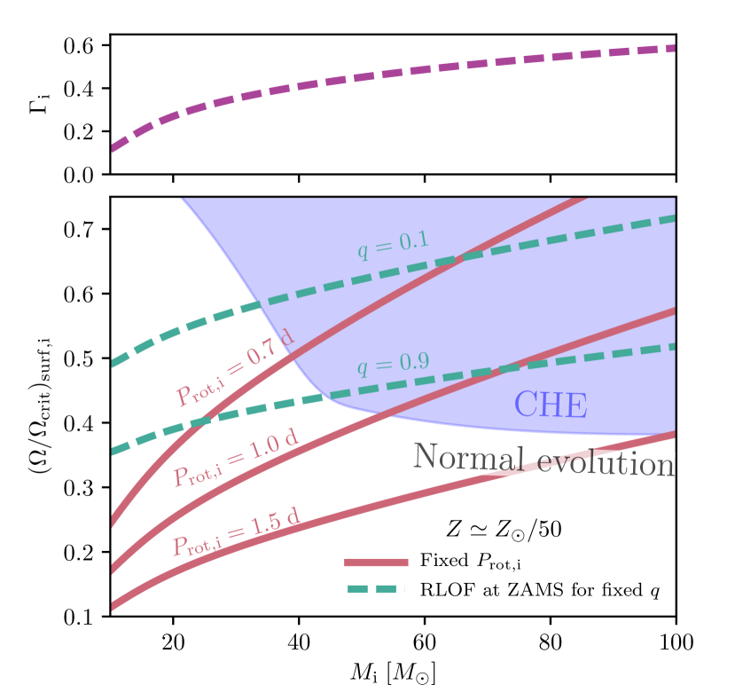
Figure 2: (top) Eddington factor at the ZAMS for non-rotating stars at a metallicity $Z=10^{-3.5}\simeq Z_{\odot}/50$. (bottom) Initial conditions for the occurrence of CHE in single stars at the same metallicity, in terms of mass at the ZAMS and initial ratio of angular frequency $\Omega$ to its critical value $\Omega_{\rm crit}$ at the surface. The colored region indicates stars for which the surface helium abundance at TAMS exceeds 0.8 and is a sharp transition. Solid lines correspond to a fixed initial rotational period, while dashed lines indicate the value of $\Omega/\Omega_{\rm crit}$ if the star is the primary of a binary system at a fixed mass ratio $q$ which exactly fills its Roche lobe at the ZAMS (see Equation 9).

Despite the reduction in stellar lifetimes with mass, rotational mixing is expected to play a larger role for the more massive stars, owing to the increasing importance of radiation pressure which reduces the stability of the stratification in the radiative envelope (Yoon et al., 2006), and to the larger mass of the convective cores relative to the total mass (see, eg. Köhler et al., 2015). This makes the threshold $\Omega/\Omega_{\rm crit}$ for efficient mixing decrease with mass. In contrast, $\Omega_{\rm crit}$ at the ZAMS decreases with mass, so at a constant initial rotation period $\Omega/\Omega_{\rm crit}$ increases with mass, as is shown by the solid lines in Figure 2. If we consider a binary with tidally locked components, this means that for mass ratios close to unity both stars can be inside the region for CHE, while for lower mass ratios the less massive component would evolve normally.

Another important point is that to form a ULX the binary has to avoid RLOF before the primary forms a BH. This again is in contrast to the binary-BH formation channel with CHE, where the detailed simulations of Marchant et al. (2016) showed that most systems need to be in contact to undergo efficient rotational mixing. If the primary is tidally locked such that its rotational frequency is $\Omega=\sqrt{G(M_{1}+M_{2})/a^{3}}$, the largest possible value that $\Omega/\Omega_{\rm crit}$ can have while avoiding mass transfer results when the primary is filling its Roche lobe ($R_{1}=R_{\rm RL,1}=f(q)a$). In this case $\Omega/\Omega_{\rm crit}$ is only a function of the mass ratio and $\Gamma$,

$$\left(\frac{\Omega}{\Omega_{\rm crit}}\right)_{\rm max}=\sqrt{\frac{(1+q)f(q)^{3}}{1-\Gamma}},$$ (9)

which is equal to $0.46(1-\Gamma)^{-1/2}$ and $0.33(1-\Gamma)^{-1/2}$ for $q=0.1$ and $q=0.9$ respectively. This is shown with dashed lines in Figure 2 and it explains why binaries with lower mass ratios can experience CHE while avoiding contact (cf. Yoon et al., 2006; de Mink et al., 2009). For lower mass ratios, binaries can have shorter orbital periods without undergoing RLOF, allowing for a larger range of systems where the primaries fall into the CHE region. The requirement of having a system that avoids RLOF at the ZAMS also limits the minimum primary mass at which CHE evolution can happen in a binary. In all of our binary simulations, the least massive primary that evolves chemically homogeneously has an initial mass $M_{1}=45M_{\odot}$.

Although Figure 2 is useful to illustrate the requirements for CHE in a binary system, this boundary depends on how rotation rates change due to mass loss through the full main sequence evolution, and this is different for single and binary stars. In a tidally synchronized binary, changes in the rotational period depend on how mass loss alters the orbital period, and this is mass-ratio dependent. To assess whether a binary would undergo CHE we then need to model each individual system in detail. In what follows, we describe in more detail how a ULX is formed through CHE, what sets the lower and upper limits in mass ratio for the formation of ULXs, and discuss the effect of metallicity on this channel.

3.1 Mass-ratio dependence and sample case of ULX formation

To exemplify the formation of a ULX via CHE, let us consider the evolution of systems with metallicity $Z=10^{-3.5}\simeq Z_{\odot}/50$ and primary mass $M_{1}=70M_{\odot}$ as the example shown in Figure 1, but for three different mass ratios $q=0.05,0.2$ and $0.6$. For a mass ratio $q=0.05$ (a secondary mass of $3.5M_{\odot}$) and an initial period of $0.8\leavevmode\nobreak\ {\rm days}$, the primary is close to filling its Roche-lobe at the ZAMS, with $R/R_{\rm RL}\simeq 0.92$. However, this binary would have an initial orbital separation of $15R_{\odot}$, while the minimum separation at which the system would avoid the Darwin instability is $a_{\rm Darwin}=21R_{\odot}$. Because of this we do not expect this system to be formed, as it would have resulted in a merger instead of a tidally synchronized binary which is our assumed initial state.

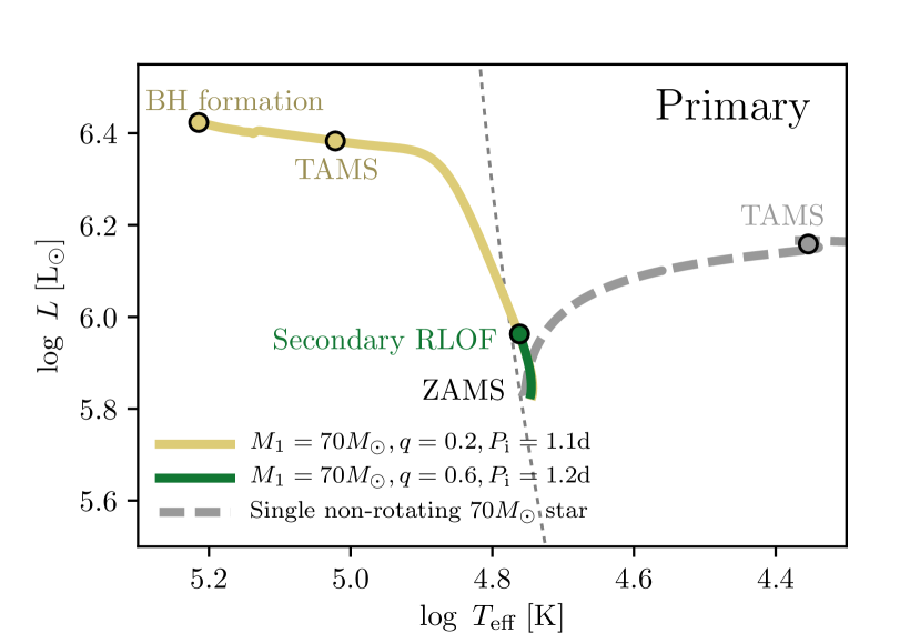
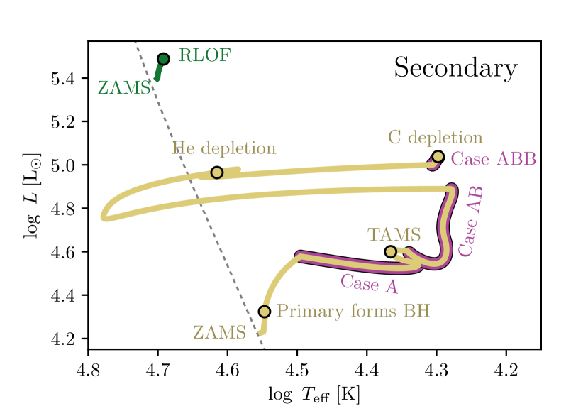
Figure 3: Evolution in the Hertzsprung-Russell diagram of the primary (top) and secondary (bottom) stars in binary systems with $Z=10^{-3.5}\simeq Z_{\odot}/50$ consisting of a $70M_{\odot}$ primary with mass ratios $q=0.2,0.6$ and initial orbital periods that are close to producing RLOF at the ZAMS. The dotted line shows the location of the ZAMS for non-rotating stars, and the track of a non-rotating $70M_{\odot}$ star is also shown for reference. The system with initial mass ratio $q=0.6$ has the primary evolving chemically homogeneously, but the secondary initiates mass transfer before a BH is formed. The system with initial $q=0.2$ manages to form a BH and afterwards undergoes three distinct phases of mass transfer. See Section 3.1 for details.

At larger initial mass ratios the initial configuration is not Darwin unstable, and we show in Figure 3 the evolution in the Hertzsprung-Russell diagram for two systems with mass ratios $q=0.2$ and $0.6$. For an initial mass ratio $q=0.6$ (a secondary mass of $42M_{\odot}$) and an initial period of $1.2\leavevmode\nobreak\ {\rm days}$, after $1.6\leavevmode\nobreak\ {\rm Myrs}$ the orbital separation is still $1.2\leavevmode\nobreak\ {\rm days}$, and the primary experiences a significant amount of mixing, with $Y_{\rm c}=0.44$ and $Y_{\rm s}=0.35$. However, the secondary does not evolve homogeneously, and by this point it has expanded enough to undergo RLOF. Since the secondary is the less massive component, mass transfer will widen the orbit and transfer hydrogen-rich material on the surface of the primary. The steep change in mean molecular weight at the base of the accreted material prevents it from mixing inwards, so we terminate the simulation as we expect the system to break away from CHE.

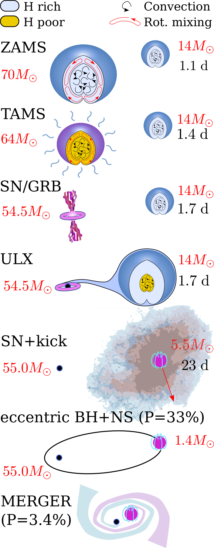
Figure 4: Schematic evolution of a ULX model arising from CHE of the more massive component in a compact binary with unequal masses and $Z=10^{-3.5}\simeq Z_{\odot}/50$ (see Section 3.1 for details). The phase of RLOF actually corresponds to three distinct mass-transfer phases. If at the moment of formation of the NS (or BH for the most massive secondaries) there is a kick in a favorable direction, a compact enough system can be formed such that a merger is possible in less than a Hubble time. For this system in particular, assuming a Maxwellian kick distribution with 1D root-mean-square $\sigma=265\leavevmode\nobreak\ {\rm km\leavevmode\nobreak\ s^{-1}}$, there is a $67\%$ chance that the binary is disrupted, and a $3.4\%$ chance that it results in a NS+BH merger in less than a Hubble time. For simplicity, mass loss at the moment of formation of the first BH is ignored.

To form a ULX, a system with a mass ratio high enough to avoid the Darwin instability, but small enough to avoid interacton before forming a BH is needed. This is the case for the system shown in Figure 4, depicting the evolution for an initial mass ratio $q=0.2$ and an initial period of $1.1\leavevmode\nobreak\ {\rm days}$. The primary in this system evolves chemically homogeneously, depleting central helium after $4.6\leavevmode\nobreak\ {\rm Myrs}$. At this point the orbital period has slightly increased to $1.7\leavevmode\nobreak\ {\rm days}$, but more importantly, the secondary has barely evolved, and its core hydrogen mass fraction is $X_{\rm c}=0.62$. At core helium depletion the primary is still rapidly rotating, with a dimensionless spin angular momentum $a_{0}=1.25$ and a mass of $55M_{\odot}$. As discussed in Section 2.3, we ignore the possibility of a PPISN or a LGRB, and assume the star collapses directly into a $55M_{\odot}$ BH with $a=1$. $12.6\leavevmode\nobreak\ {\rm Myrs}$ after the formation of the system, and with $X_{\rm c}=0.24$, the secondary overflows its Roche-lobe and undergoes a phase of Case A mass transfer lasting $1.6\leavevmode\nobreak\ {\rm Myrs}$, and reducing its mass from $14M_{\odot}$ to $8.6M_{\odot}$, while widening the orbit from $1.7$ to $6.5$ days. The typical mass-transfer rate during this phase is $\leavevmode\nobreak\ \dot{M}_{\rm mt}=10^{-5.7}\leavevmode\nobreak\ M_{\odot}\leavevmode\nobreak\ {\rm yr^{-1}}$, which is only a factor of five above the Eddington rate of the BH. The Eddington luminosity of the BH exceeds $8\times 10^{39}\leavevmode\nobreak\ \rm erg\leavevmode\nobreak\ s^{-1}$, so during mass transfer the system would be an ultra-luminous X-ray source.

After the secondary depletes its central hydrogen, it expands to undergo a short-lived phase (lasting only $28000\leavevmode\nobreak\ {\rm yrs}$) of Case B mass transfer which reduces its mass to $5.8M_{\odot}$, with mass-transfer rates as high as $\dot{M}_{\rm mt}=10^{-3.4}\leavevmode\nobreak\ M_{\odot}\leavevmode\nobreak\ {\rm yr^{-1}}$. At detachment the orbital period is $20\leavevmode\nobreak\ {\rm days}$, and the star has a helium core of $3.6M_{\odot}$, with a significant hydrogen-rich envelope left. During core helium burning most of the envelope is turned into pure helium, resulting in a $5.8M_{\odot}$ star with a $5.1M_{\odot}$ hydrogen-depleted core. After helium depletion, the remaining envelope expands and manages to initiate Case BB mass transfer; however carbon ignites during mass transfer and is rapidly depleted after only $0.3M_{\odot}$ is transferred, though this is already enough to increase the orbital period to $23\leavevmode\nobreak\ {\rm days}$. Note that the overall efficiency of all mass-transfer phases is low, with the BH increasing its mass only by $0.5M_{\odot}$. Assuming the $5.5M_{\odot}$ star explodes as a SN with a possibly strong kick oriented in a random direction, there is a small chance ($3.4\%$) that the system remains in a tight and very eccentric orbit that would allow a BH-NS merger within a Hubble time (see Section 6).

In general, considering our complete set of simulations, we find that ULXs can be formed for initial mass ratios in the range $q\simeq 0.1-0.45$. The lower limit on mass ratios is a product of the Darwin instability, while the upper limit results because secondaries initiate RLOF before BH formation, interrupting CHE. For reference, the detailed outcomes of all our models are shown in Appendix A.

3.2 The impact of metallicity on the properties of ULXs

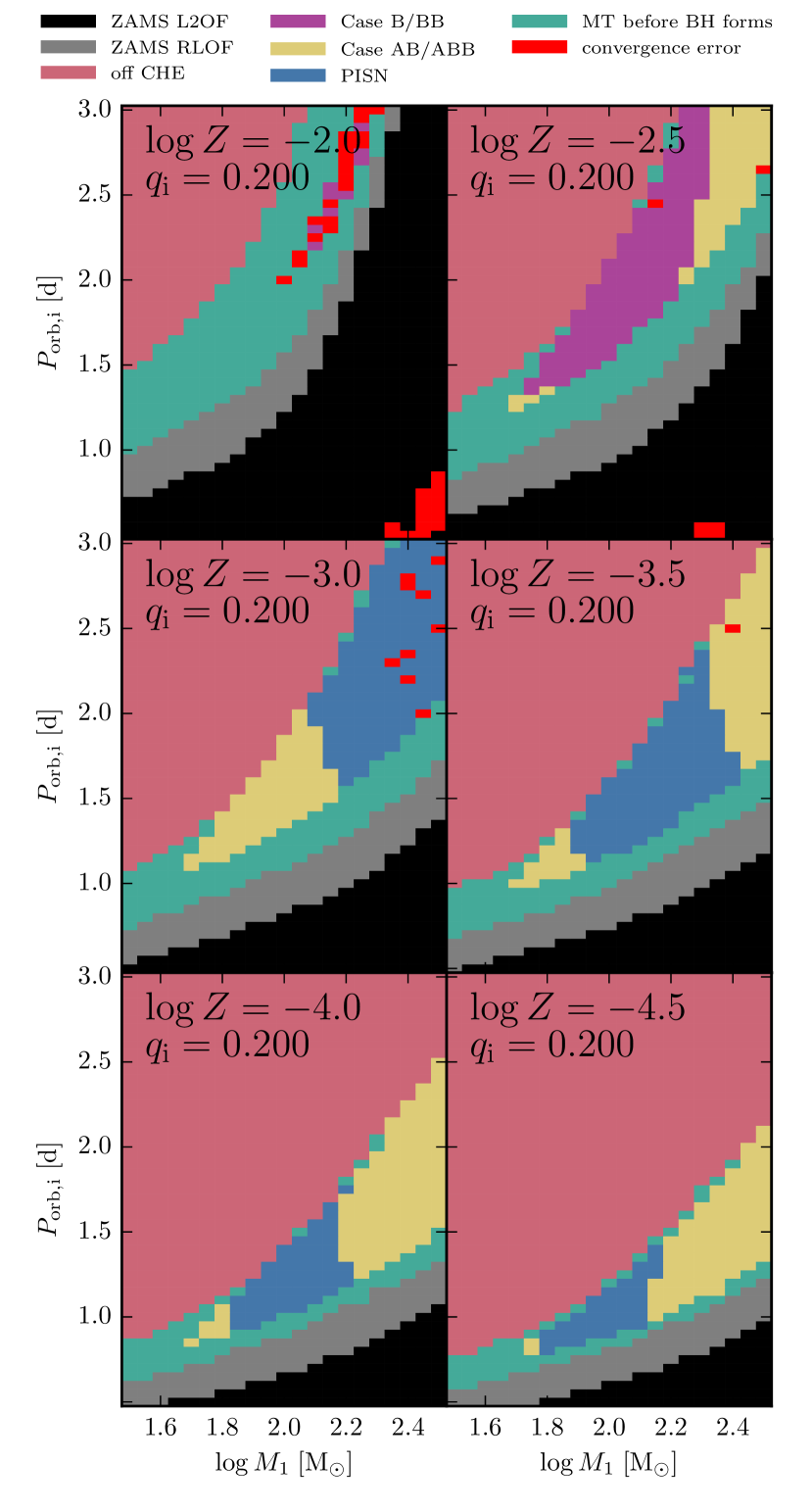
Figure 5: Outcome of simulations for different metallicities and a fixed mass ratio $q$. Systems marked as Case B/BB or Case AB/ABB have primaries that evolve chemically homogeneously and form BHs, to which the secondary then transfers mass resulting in a ULX. Systems marked in blue have primaries that evolve chemically homogeneously but have final masses resulting in PISNe. All other systems interact before the formation of a BH and would not form a ULX. See Appendix A for the outcome of all simulations. and a detailed description of all outcomes.

Figure 5 shows the outcome of simulations with $q=0.2$ for some of the metallicities modeled. At a fixed mass ratio and metallicity, the initial primary masses and orbital periods for which the primary can evolve chemically homogeneously are very similar to those that can produce binary BHs from initial mass ratios closer to unity (Marchant et al., 2016), the main difference being that the period window for contact-less evolution is much larger. Although wind mass loss typically disfavors CHE as it brakes the star’s rotation, for the most massive primaries it can help expose helium-enriched layers from their large convective cores, significantly widening the window for this channel at the highest masses (Köhler et al., 2015; Szécsi et al., 2015).

The properties of ULXs produced through CHE are strongly dependent on metallicity. Metal-poor stars are more compact, making it possible for binaries with the same component masses to have shorter initial orbital periods while still avoiding RLOF at the ZAMS, as can be seen in Figure 5. Although shorter initial orbital periods result in faster surface rotation velocities, this does not translate into more systems undergoing CHE, as the relevant quantity to consider mixing efficiency is not the absolute rotational velocity, but rather its ratio to the critical velocity, which also increases as stars become more compact at lower metallicity. The effect of metallicity-dependent mass loss is more complex. For the highest metallicity modeled, $Z=0.01$, mass loss results in significant orbital widening, which together with tidal coupling significantly spins down the primary and results in very few systems evolving chemically homogeneously. In contrast, for extremely low metallicities, reduced winds mean that the window for the channel does not widen too much at the highest masses.

For systems undergoing CHE, mass loss determines the occurrence of PISNe. At $\log\leavevmode\nobreak\ Z=-2.5$, mass loss is strong enough that systems with initial masses of $300M_{\odot}$ result in helium cores below $60M_{\odot}$, avoiding explosion as a PISNe and producing BHs. At a metallicity of $\log\leavevmode\nobreak\ Z=-3$, the most massive primaries have final masses well above $60M_{\odot}$, which we would expect to explode as PISNe. At $\log\leavevmode\nobreak\ Z=-3.5$ mass loss has reduced to the point where we get primaries with final masses above $130M_{\odot}$, that could possibly avoid the PISNe fate and instead produce very massive BHs. This would translate into a gap in BH masses. At even lower metallicities, the region where PISNe occur moves further down in terms of initial primary mass, and as mass loss becomes negligible, the period window for CHE becomes narrower. This narrowing increases the minimum primary mass at which CHE occurs, such that at an extremely low metallicity of $\log\leavevmode\nobreak\ Z=-6$ only primaries above $70M_{\odot}$ undergo CHE. As mass loss is very weak, these stars still fall into the mass range for PISNe, and there is no longer a gap in BH masses; all the resulting BHs come from systems above the mass limit for PISNe.

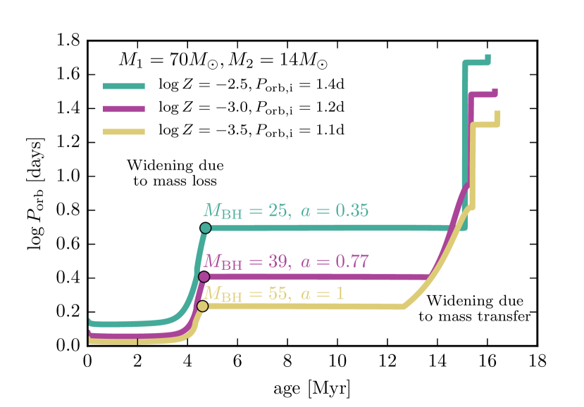
Figure 6: Orbital separation as a function of time for three different systems with the same initial component masses and different metallicities. The initial periods correspond to the shortest one in our simulations for which a system with those component masses and metallicity evolves chemically homogeneously and undergoes a ULX phase. Circles mark the moment of BH formation, and the initial mass and spin of the BH are shown.

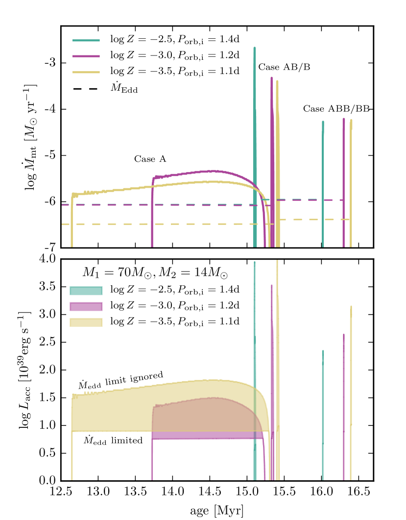
Figure 7: Mass-transfer rates and accretion luminosities during mass-transfer phases for the three systems shown in Figure 6. Accretion luminosities are shown as ranges going from the lower values given by strictly Eddington limited accretion rates, to the potential luminosities that could be achieved if the Eddington limit is ignored. Note that the Eddington accretion rates for the metallicities $\log\leavevmode\nobreak\ Z=-2.5$ and $-3$ overlap. This is due to the lower BH spin at $\log\leavevmode\nobreak\ Z=-2.5$ compensating for the higher BH mass at $\log\leavevmode\nobreak\ Z=-3$.

Mass loss of the primary star also affects the lifetime of a possible ULX phase. Figures 6 and 7 show the evolution of the orbital period and the mass-transfer phases for three of our ULX models with initial primary masses of $70M_{\odot}$ and metallicities $\log\leavevmode\nobreak\ Z=-2.5,-3$ and $-3.5$. The highest metallicity model widens significantly due to mass loss before the BH forms, resulting in the secondary initiating RLOF only after core hydrogen depletion. This Case B mass-transfer phase is short-lived, making it unlikely to detect ULXs during this phase of evolution. In contrast, the two lower metallicity systems remain compact enough after BH formation to undergo long-lived phases of nuclear-timescale mass transfer, with the duration of these increasing at lower metallicities as the orbit widens less and mass transfer starts earlier while the secondary undergoes core-hydrogen burning. The resulting luminosities for these Case A systems are well above $10^{39}\leavevmode\nobreak\ {\rm erg\leavevmode\nobreak\ s^{-1}}$ even when strictly limited to the Eddington rate. During Case A, mass-transfer rates are not much higher than the Eddington rate, which means that even if the Eddington limit is ignored, luminosities can only increase by a factor of $\sim 5$. The situation is different during Case AB/B and ABB/BB mass transfer, where mass-transfer rates can go many orders of magnitude above $\dot{M}_{\rm Edd}$, resulting in potential luminosities going above $10^{42}\leavevmode\nobreak\ {\rm erg\leavevmode\nobreak\ s^{-1}}$, which is the range for HLXs. However, achieving these luminosities requires a complete disregard of the Eddington limit, and even then, the short lifetimes involved would likely make these sources very rare. Note that, with mass accretion limited to the Eddington rate, the BHs modeled have only modest increases in their total masses and spins. The small increase in $\dot{M}_{\rm Edd}$ that can be observed during Case AB/B mass transfer in Figure 7 is only due to a decrease in the opacity of accreted material, as helium rich layers from the secondary are exposed.

4 Luminosity distribution function of ULXs

To estimate the expected properties of observed ULX samples at a fixed metallicity, we need to assume certain distribution functions describing the population of binaries at zero age. We follow the choices made by Marchant et al. (2016), which consider a Salpeter distribution for primary masses ($dN/dM_{1,\rm i}\propto M_{1,\rm i}^{-2.35}$), a flat distribution in $\log\leavevmode\nobreak\ P_{\rm orb}$ ranging from $0.5$ days to a year, a flat distribution in mass ratio from zero to unity, and a binary fraction $f_{b}=0.5$ (i.e. out of three massive stars two form part of a binary system). If we assume the threshold mass for SNe is $8M_{\odot}$, and that the SN rate is $10^{-2}\leavevmode\nobreak\ {\rm yr^{-1}}$ for a star-formation rate (SFR) of ${\rm 1M_{\odot}\leavevmode\nobreak\ yr^{-1}}$, we can then compute expected distributions of luminosities per $M_{\odot}\leavevmode\nobreak\ {\rm yr^{-1}}$ of SFR. This choice for the rate of SNe per $M_{\odot}\leavevmode\nobreak\ {\rm yr^{-1}}$ of SFR is consistent with Milky Way values (Diehl et al., 2006; Robitaille & Whitney, 2010). Note that the distributions we obtain depend linearly on this assumed ratio between the supernova rate and the SFR, which is uncertain to at least a factor of $2$. A detailed description of how we derive formation rates and observable numbers of ULXs is provided in Appendix B.

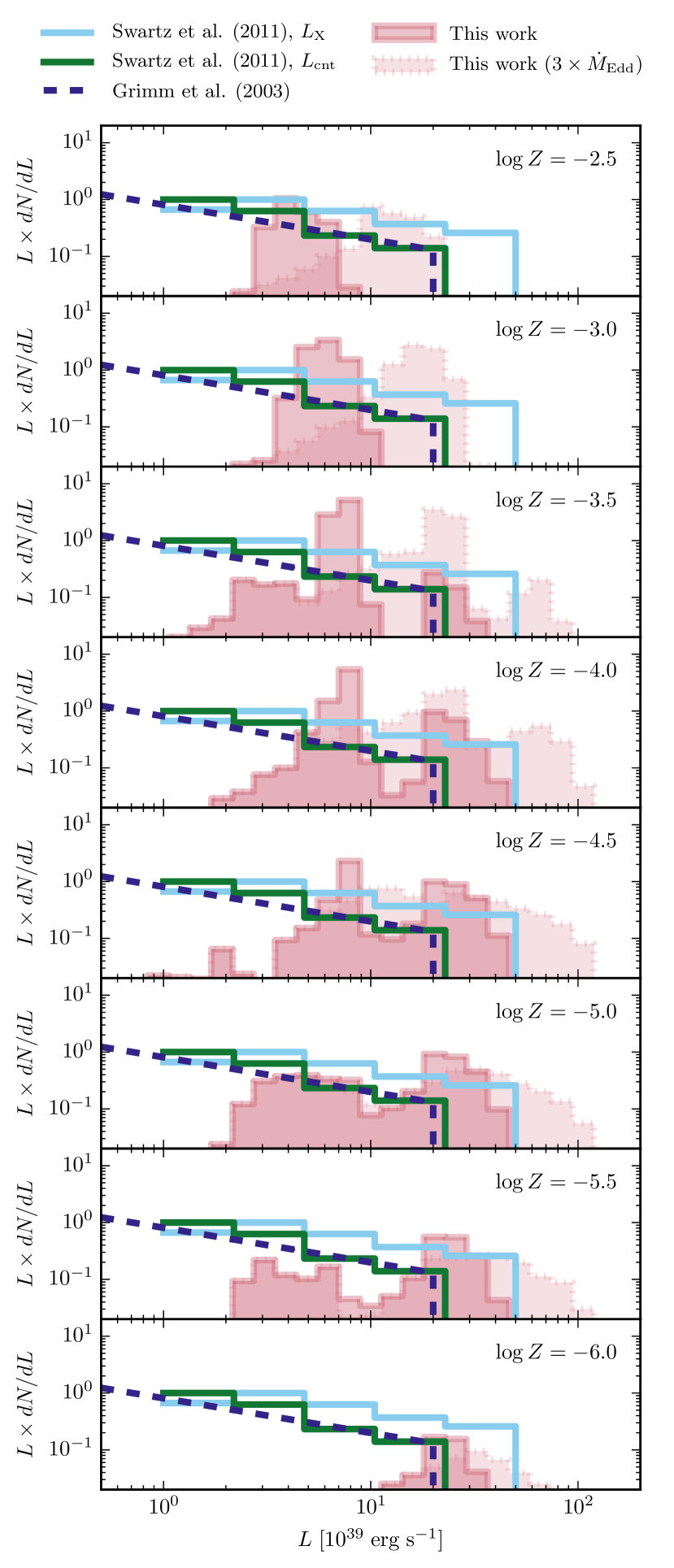
Figure 8: Expected luminosity distribution function for ULXs formed through CHE, compared to the empirical distribution with a slope $\alpha=-1.6$ derived by Grimm et al. (2003) and the sample of 117 ULXs from nearby galaxies described by Swartz et al. (2011), both of which cover metallicities $\log Z>-3.0$. For the sample of Swartz et al. (2011) we include the distributions considering their estimates on source luminosities from spectral modelling $L_{\rm X}$, and that from number of counts $L_{\rm cnt}$. All distributions are normalized to a star-formation rate of ${1\leavevmode\nobreak\ M_{\odot}\leavevmode\nobreak\ \rm yr^{-1}}$.

Figure 9: Same as Figure 8 but for the cumulative distribution function instead. Expected number of observable sources per $M_{\odot}\leavevmode\nobreak\ {\rm yr^{-1}}$ of SFR are also shown, as well as the expected formation rate of ULXs in terms of the SN rate. Although the number of ULXs produced per SN increases with metallicity, at lower metallicities phases with accretion are longer lived resulting in a peak in observable sources per $M_{\odot}\leavevmode\nobreak\ {\rm yr^{-1}}$ of SFR at $\log\leavevmode\nobreak\ Z=-4$.

Our predicted luminosity distribution function and cumulative distribution function are shown in Figures 8 and 9, respectively. These take into account the lifetime of the sources modeled, so they can be compared to observed samples of ULXs. To consider possible uncertainties on the efficiency of mass transfer, we also include the distribution of luminosities if accretion rates of three times the Eddington rate would be possible. This is not done by running a full set of simulations with an adjusted Eddington limit, but rather by considering the potential luminosities of our models which are strictly limited to accrete at $\dot{M}_{\rm Edd}$. The resulting luminosities obtained in this way agree well with models computed self-consistently with an adjusted $\dot{M}_{\rm Edd}$ (see Appendix C for details). For our models we consider the full bolometric accretion luminosity $L_{\rm acc}$, although a fraction of this would not be emitted in the bands detectable by X-ray observatories.

To compare with observations, we also include the empirical distribution described by Grimm et al. (2003) for nearby (within $35\leavevmode\nobreak\ \rm Mpc$) late-type starburst galaxies, described by a power law with a slope of $\sim-1.6$, and a cutoff at a luminosity of $2\times 10^{40}\leavevmode\nobreak\ {\rm erg\leavevmode\nobreak\ s^{-1}}$. Grimm et al. (2003) and Gilfanov et al. (2004) argue that the presence of such a cutoff is indicative of a maximum possible mass for stellar BHs. We also include the 117 ULXs described by Swartz et al. (2011), which represent complete samples of ULXs for local galaxies of diverse types within $14.5\leavevmode\nobreak\ \rm Mpc$. Swartz et al. (2011) consider two different methods to compute the luminosity of ULXs, one obtained from photon counts, and the other, for sources with $>130$ counts detected, from spectral modelling. Although the luminosities from Grimm et al. (2003) correspond to the $2-10\leavevmode\nobreak\ \rm keV$ band, while the photon counts from Swartz et al. (2011) are corrected to give the luminosities in the $0.3-10\leavevmode\nobreak\ \rm keV$ range, the two samples agree well with each other.

The galaxies considered by Grimm et al. (2003) and Swartz et al. (2011) should be indicative of the formation of ULXs in the local environment of our Galaxy and favor high metallicities, with no sources below $\log Z<-3.0$. Moreover, as they do not properly sample dwarf galaxies, we expect an additional bias towards higher metallicities. In particular, there is one ULX detected in the blue compact dwarf galaxy IZw18 (Ott et al., 2005), which has a very low metallicity of $Z_{\odot}/50$, and the study of ULXs in dwarf galaxies provides hints of an increasing number of observable ULXs per $M_{\odot}\;\rm yr^{-1}$ of SFR with decreasing galaxy mass (Swartz et al., 2008).

The CHE channel is expected to produce the most massive BHs possible for a given metallicity, as it transforms almost the whole star into a large helium core. Since large initial masses are required to have efficient rotational mixing, this results in the least massive BH possible at $\log\leavevmode\nobreak\ Z=-2.5$ to have a mass of $20M_{\odot}$, already falling into the ULX range when accreting at the Eddington rate. As Figure 8 shows, there is a much less luminous tail of objects that arises from brief moments at the beginning and end of mass-transfer phases, when transfer rates are below the Eddington limit. At a metallicity of $\log\leavevmode\nobreak\ Z=-3$ we reach a luminosity cutoff due to the lower limit for PISNe at about $10^{40}\leavevmode\nobreak\ \rm erg\leavevmode\nobreak\ s^{-1}$, which, barring possible mass loss from PPISNe, means that accretion rates that are only a factor of a few above Eddington are enough to explain the observed luminosity cutoff with our models. A population of lower mass BHs and NS accretors is still required to explain the lower end of the luminosity function of ULXs, extending to the HMXB regime. Such systems are likely to originate from CE evolution, meaning that the BH accretor results from an envelope stripped star (Podsiadlowski et al., 2003), and thus should have lower masses than those possible through CHE. Although the inclusion of a different channel should in principle produce a break in the distribution function, a similar break that should be visible due to differences between NS and BH accretors is not observed (Grimm et al., 2003), and the distribution function for our highest metallicity models is not far off from that of the most luminous objects in the observed sample. It might be possible then that the population of NS and BH accretors resulting from CE evolution coexists with those produced by CHE and results in a luminosity distribution function that can be described with a single slope.

At lower metallicities this should not be the case; Figure 8 shows that a gap in the luminosity function is expected. This is due to the formation of BHs above the limit for PISNe. The gap is not completely deserted, as systems at the beginning or end of mass-transfer phases to those very massive BHs accrete below the Eddington rate, resulting in a wide range of luminosities for a short period of time. This gap in the distribution results in a clear feature in the cumulative distribution, as shown in Figure 9. Observations in the local universe would favor the observation of galaxies at the upper end of the metallicities modelled, but deeper observations sampling lower metallicity environments should show a significant digression from a population describable by a single power law.

In terms of observable sources, the CHE channel has a strong dependence on metallicity, with almost no sources being produced at metallicities $Z\geq 0.01$, and rising to a peak of $2.3$ ULXs per $M_{\odot}\leavevmode\nobreak\ {\rm yr^{-1}}$ of SFR at a metallicity of $\log\leavevmode\nobreak\ Z=-4$, though the rate is mostly flat in the range $-4.5<\log\leavevmode\nobreak\ Z<-3$. In a slightly counterintuitive way, at metallicities below $\log\leavevmode\nobreak\ Z=-2.5$ the number of ULXs formed per SNe monotonically decreases with metallicity, but it has to be taken into account, as described in Section 3.2, that due to orbital widening from wind mass loss, mass-transfer phases have shorter lifetimes at higher metallicities. This compensates for the smaller number of sources produced per SN at lower metallicities, resulting in the local maximum of observable sources at $\log\leavevmode\nobreak\ Z=-4$. Anyhow, with just a couple of systems formed every $10^{4}$ SNe, it is clear that this evolution channel is only followed by a small fraction of massive stars. Although there are important uncertainties in our calculations, in particular in the choice of initial distribution functions at low metallicities, this systematic behaviour with metallicity should be a generic feature, despite uncertainties of at least a few in the rates we predict.

4.1 Luminosity distribution at redshift $z=0$

Figure 10: Same as Figures 8 and 9, but weighting our models according to the metallicity distribution of Langer & Norman (2006) at redshift $z=0$.

It is tempting to relate the predicted rate of $\sim 2$ ULXs per $M_{\odot}\leavevmode\nobreak\ {\rm yr^{-1}}$ of SFR with the equivalent observed number of sources by Swartz et al. (2011), but we need also consider the contribution from the tail of the normal HMXB population that reaches up to ULX luminosities. More importantly, both the Swartz et al. (2011) and Grimm et al. (2003) sources sample the local universe. If we consider the metallicity distribution of Langer & Norman (2006) evaluated at a redshift $z=0$, we would only expect $\sim 1\%$ of the star-formation in the local universe to happen at a metallicity below $\log\leavevmode\nobreak\ Z=-3$. We use this distribution to evaluate the local luminosity distribution function of ULXs formed through CHE, which we show in Figure 10. The metallicity weighting significantly reduces the number of expected sources to $0.13$ ULXs per $M_{\odot}\leavevmode\nobreak\ {\rm yr^{-1}}$ of SFR, but if we consider mass accretion at three times the Eddington rate, the distribution we predict nicely matches that of the brightest sources of Grimm et al. (2003) and of Swartz et al. (2011) estimated by photon counts. For the majority of ULXs which have lower luminosities, a different formation channel would be required. The luminosities estimated by Swartz et al. (2011) through spectral modeling should better represent the total luminosity of the source, which is what we consider for our models. However, if accretion rates ten times larger than Eddington are allowed to try to match these higher luminosities, Figure 10 shows that the gap produced by PISNe is lost. This is because not many systems transfer mass at those high rates (see Table 1), so the luminosity distribution does not simply shift to higher luminosities. If the increased luminosity is due to a relatively constant beaming factor rather than accretion above the Eddington rate, then we expect that luminosity gap would remain. In any case, the spectrum of BHs $<60M_{\odot}$ and $>130M_{\odot}$ radiating at the same luminosity should differ significantly.

$\log\leavevmode\nobreak\ Z$	$\displaystyle\frac{n_{\rm ULX}}{\rm SFR}\leavevmode\nobreak\ {[M_{\odot}^{-1}\leavevmode\nobreak\ \rm yr]}$			%$>3\dot{M}_{\rm Edd}$	%$>10\dot{M}_{\rm Edd}$	$\displaystyle\frac{R_{\rm ULX}}{R_{\rm SN}}\times 10^{4}$			$\langle t_{\rm ULX}\rangle\leavevmode\nobreak\ \rm[Myr]$	$\displaystyle\left\langle\frac{L_{\rm X,gal}}{\rm SFR}\right\rangle\leavevmode\nobreak\ {\left[\frac{10^{39}\leavevmode\nobreak\ {\rm erg\leavevmode\nobreak\ s^{-1}}}{M_{\odot}\leavevmode\nobreak\ {\rm yr}^{-1}}\right]}$
-2.5	0.6	(0.6,	0)	71	25	2.6	(2.6,	0)	0.23	2.6
-3.0	1.9	(1.9,	0)	76	16	1.9	(1.9,	0)	1	11
-3.5	2.2	(2.1,	0.12)	67	16	0.98	(0.71,	0.26)	2.2	17
-4.0	2.3	(1.8,	0.51)	39	2.1	1.0	(0.44,	0.58)	2.3	26
-4.5	1.5	(0.77,	0.7)	7.7	1.7	0.78	(0.18,	0.61)	1.9	22
-5.0	1.1	(0.45,	0.64)	5.3	1.5	0.66	(0.13,	0.53)	1.7	17
-5.5	0.56	(0.18,	0.39)	5.2	1.4	0.34	(0.044,	0.29)	1.6	9.9
-6.0	0.11	(0,	0.11)	2.6	0.85	0.067	(0,	0.067)	1.6	2.3
local	0.13	(0.13,	0.00062)	70	21	0.39	(0.39,	0.0011)	0.33

Table 1: Rates and general properties of ULXs formed through CHE at different metallicities. Shown here are the expected number of observable ULXs $n_{\rm ULX}$ per $M_{\odot}\leavevmode\nobreak\ {\rm yr^{-1}}$ of SFR, the number of produced ULXs per SNe (i.e. the ratio between the formation rates of ULXs, $R_{\rm ULX}$, and SN, $R_{\rm SN}$), and the expected total X-ray luminosity of galaxies (from sources produced through CHE) per $M_{\odot}\leavevmode\nobreak\ {\rm yr^{-1}}$ of SFR. In parenthesis we indicate separately the number of objects with BHs below the pair-instability gap ($M_{\rm BH}<60M_{\odot}$) and above it ($M_{\rm BH}>130M_{\odot}$). Also included for the expected number of observable ULXs is the percentage of those systems that would accrete at 3 and 10 times their Eddington rates, while for the formation rates we include the average time that formed ULXs spend as such, $\langle t_{\rm ULX}\rangle$. The last column is computed under the assumption that the bolometric luminosity from accreting sources is released as X-rays, and that accretion is strictly limited to the Eddington rate. Local rates are estimated using the metallicity distribution of Langer & Norman (2006) at redshift $z=0$. A value for the locally weighted galactic $L_{\rm X,gal}$ is ignored, as the local environment contains many galaxies at higher metallicities where the total luminosity would be dominated by HMXBs instead of the ULXs described in this work. Values given in terms of SFR are computed assuming a SN rate of $0.01\leavevmode\nobreak\ \rm yr^{-1}$ per $1M_{\odot}\leavevmode\nobreak\ \rm yr^{-1}$ SFR.

Locally, ULXs with BH masses $>130M_{\odot}$ would only represent a small fraction of the total formed through CHE, around $\sim 0.5\%$. Moreover, since ULXs formed through this channel only represent the high-luminosity tail of the luminosity distribution function, they correspond to an even smaller fraction of the total. The upcoming eROSITA X-ray observatory will perform a full-sky survey, which at a sensitivity limit of around $2\times 10^{-14}\leavevmode\nobreak\ \rm erg\leavevmode\nobreak\ s^{-1}\leavevmode\nobreak\ cm^{-2}$ should detect sources with luminosities of $10^{40}\leavevmode\nobreak\ \rm erg\leavevmode\nobreak\ s^{-1}$ up to a distance of $35\leavevmode\nobreak\ \rm Mpc$. Considering the distribution of known sources, around $\sim 100$ ULXs should be detected (Prokopenko & Gilfanov, 2009), so that finding BHs above the PISN gap would appear unlikely. However, as shown in Figure 10, if BHs above the PISN gap can accrete at rates above a few times $\dot{M}_{\rm Edd}$ their luminosities would approach $10^{41}\leavevmode\nobreak\ \rm erg\leavevmode\nobreak\ s^{-1}$, with significantly larger detection volumes (for sources three times more luminous than the cutoff luminosity the detection volume would be $\sim 5$ times larger). eROSITA could then potentially detect a few of these sources, likely in metal-poor dwarf galaxies. On a longer timescale, the Athena X-ray observatory will be capable of probing much deeper, and targeted observations to dwarf galaxies with very low metallicities and high SFRs could test the existence of these objects.

4.2 $L_{\rm X,gal}-\rm SFR$ relation at low metallicities

As we predict the luminosity distribution of X-ray sources to change significantly at low metallicities, we also expect the relation between the total X-ray luminosity of a galaxy $L_{\rm X,gal}$ and its SFR to be different from that in our local environment. Locally, the X-ray luminosity of a galaxy serves as a probe of its SFR (Grimm et al., 2003; Gilfanov et al., 2004), and the presence of a luminosity cutoff results in a linear $L_{\rm X,gal}-\rm SFR$ relationship for high enough SFR. Gilfanov et al. (2004) argue that a population of IMBHs would result in a break from the linear relationship at very high SFR. As BHs formed above the limit for PISNe also form a distinct population of very massive BHs, they could as well result in differences in the dependence of $L_{\rm X,gal}$ with SFR. Moreover, if the $L_{\rm X,gal}-\rm SFR$ relationship changes significantly at lower metallicities, it would need to be recalibrated to serve as a probe of star-formation.

Figure 11: $L_{\rm X,gal}-{\rm SFR}$ relationship arising from ULXs produced through CHE at two different metallicities, compared to the predicted metallicity-independent relationship from Grimm et al. (2003) for the luminosity in the $2-10$ keV band. Systems at $\log\leavevmode\nobreak\ Z=-4$ can also produce BHs above the pair instability gap, resulting in the slightly different structure at low SFR. For simplicity we assume all the luminosity from accretion is emmited as X-rays. For different values of the SFR modelled we constructed 10000 synthetic galaxies, and the color plor indicates the fraction of galaxies contained around the median (i.e., the $20\%$ region is bounded by the fourth and sixth deciles).

To assess the $L_{\rm X,gal}-{\rm SFR}$ relationship, using our ULX models we construct multiple synthetic galaxies for different SFRs (see Appendix D for details), for which we show the distribution of X-ray luminosities in Figure 11. For galaxies with low star-formation rates, that on average should have less than one ULX produced through CHE, low-number statistics plays an important role, and this effect can clearly be seen at SFRs less than $1\leavevmode\nobreak\ M_{\odot}\leavevmode\nobreak\ \rm yr^{-1}$. Unlike the relationship observed by Grimm et al. (2003), Figure 11 shows a very steep increase in luminosity at low SFRs, but this is just because our models do not include the contribution from HMXBs. Instead, the luminosities jump from zero to above $10^{39}\leavevmode\nobreak\ {\rm erg\leavevmode\nobreak\ s^{-1}}$ for galaxies that happen to have a single ULX. Although we cannot properly assess the relationship at very low SFRs, the switch from a non-linear to a linear relationship depends on the sampling of the most luminous sources possible, and we expect ULXs formed through CHE to be the source of these. The SFR at which Grimm et al. (2003) observe a break in the X-ray luminosity distribution of galaxies would then be equivalent to the SFR at which most galaxies would sample a few of the ULXs produced through CHE.

Figure 11 shows that the SFR at which the relationship becomes linear, as well as the expected luminosities at high SFR, has an important dependence on metallicity. This results both from the increased number of sources expected per $M_{\odot}\leavevmode\nobreak\ {\rm yr^{-1}}$ of SFR at lower metallicities, and the formation of BHs above the PISNe gap which can produce much higher luminosities. Table 1 shows the ratio of $L_{\rm X,gal}$ to SFR that we expect in the linear regime at different metallicities. This value can vary up to an order of magnitude, which should be taken into account when using $L_{\rm X,gal}$ as a measure of SFR. The presence of BHs above the PISNe gap does produce changes in the $L_{\rm X,gal}-{\rm SFR}$ reationship, but this happens in the low-SFR regime, likely making it hard to observe.

5 Orbital parameters of ULXs formed through CHE

An additional tool to discriminate between different formation scenarios is the detection of optical counterparts to ULXs, which can help identify the nature of the donor star and the orbital parameters. The largest sample of counterparts to date is given by Gladstone et al. (2013), who detect potential counterparts in 22 out of 33 ULXs studied. There are also two ULXs for which dynamical estimates of the masses are available from measurements of radial-velocity variations due to the orbital motion of the donor star, detected as a WR: M101 ULX-1, with a BH mass likely in the range $20M_{\odot}-30M_{\odot}$ (Liu et al., 2013), and P13, with a BH mass below $15M_{\odot}$ (Motch et al., 2014). Both exclude the possibility of an IMBH as the compact object and set constraints on the properties of the donor. However, these dynamical mass estimates need to be considered with care, as is shown by the case of the HMXB IC10 X-1. Using measurements of radial-velocity variations, Silverman & Filippenko (2008) concluded that this system contains a BH with a mass in excess of $20M_{\odot}$, but Laycock et al. (2015) showed that the radial-velocity variation detected does not follow the stellar motion, but rather comes from a shadowed region in the stellar wind. This means that the dynamical mass estimate is incorrect, making the mass of the compact object much more uncertain and even consistent with a NS accretor.

Figure 12: (top) Distribution of BH and donor masses in ULX systems, weighting our models to the metallicity distribution of Langer & Norman (2006) at redshift $z=0$. (middle) Distribution of mass ratios using the same metallicity distribution. (bottom) Distribution of orbital periods using the same metallicity distribution. Donor masses and orbital periods are separated between Case A and Case B systems, and furthermore, Case A systems are separated between donors that are hydrogen poor or hydrogen rich at their surfaces.

It is beyond the scope of this paper to study in detail the optical properties of our ULX models and compare them to observations, which needs modeling of the emission from the accretion disk, but we can check the distribution of donor and BH masses, together with orbital periods, as is done in Figure 12. This is done by taking into account the lifetime of each phase, so it can be compared with the observed distribution. As more observations place better constraints on the orbital parameters of ULXs, their origin can be better understood by comparing those to the predicted distributions of different formation channels. The bulk ($71\%$) of ULX models formed through CHE should contain main-sequence (MS) hydrogen rich ($X_{\rm s}>Y_{\rm s}$) donors in the range $\sim 8M_{\odot}-30M_{\odot}$ with orbital periods below $20$ days. More massive MS donors in the range $30M_{\odot}-70M_{\odot}$ are only a $16\%$ of the total, with $3\%$ being hydrogen poor ($X_{\rm s}<Y_{\rm s}$). Although less numerous, these massive optical counterparts should be much easier to detect. Case AB/B systems correspond to only $6\%$ of the total, have typical donor masses below $10M_{\odot}$, and typical periods above $10$ days. As has already been mentioned, the predominance of Case A sources is owed to these systems undergoing mass transfer on a nuclear timescale, while mass transfer for post-MS donors operates on a much shorter thermal timescale.

Independent of the formation channel, a common expectation for systems undergoing RLOF is a preference for mass ratios $q=M_{2}/M_{\rm BH}$ below unity, as this value plays an important role in the lifetime of a mass-transfer phase (Podsiadlowski et al., 2003). If the donor is more massive than the BH, mass transfer typically results in a reduction of the orbital separation leading to a short-lived thermal-timescale mass transfer, similar to the situation for intermediate-mass X-ray binaries (Tauris et al., 2000). If instead the donor is a MS star less massive than the BH at the onset of mass transfer, the orbital separation increases as a result of mass transfer, leading to a much longer-lived nuclear-timescale X-ray phase.

The mass-ratio distribution for ULXs produced through CHE at redshift $z=0$ is shown in the second panel of Figure 12. Although the initial mass ratios of these systems are smaller than $q=0.5$, mass loss of the primary before BH formation can lead to mass ratios above unity during the ULX phase; but these are disfavored for the same reason discussed above. The distribution favors mass ratios significantly below unity, with $\sim 50\%$ of the sources having $q<0.5$. This preference for lower mass ratios is stronger at lower metallicites, as the primary undergoes a smaller amount of mass loss before forming a BH and preserves its initially low mass ratio. Instead, for the CE channel, the primary which will form the BH expands and initiates a CE phase, and for very low secondary masses, a merger is expected rather than envelope ejection (see, e.g. Kruckow et al., 2016). As a consequence, the distribution of mass ratios predicted from CE evolution favors mass ratios below, but nor far, from unity (Madhusudhan et al., 2008). In the case of ULXs formed via dynamical capture in clusters, much higher BH than donor masses are also expected, but the orbital periods of these systems are well above $20$ days (Mapelli & Zampieri, 2014), which differentiates them from the bulk of systems produced through CHE. The long orbital periods imply that such systems would have post-MS donors with short lifetimes as active sources, which reduces the likelihood of observing them.

The models of Madhusudhan et al. (2008) have an upper limit of $25M_{\odot}$ for the BH mass, which makes it difficult to explain some of the brightest optical counterparts observed that would require $\sim 50M_{\odot}$ donors. In consequence, they favor IMBHs as the compact object in these sources, which would allow for long-lived mass transfer phases due to the lower mass ratios. This could be avoided if CE could produce higher mass BHs, but even at low metallicities it is difficult to reach BH masses well above $30M_{\odot}$, as envelope stripping significantly reduces the mass of the primary (Linden et al., 2010). ULXs formed through CHE can reach BH masses up to the lower end of the PISN gap ($60M_{\odot}$), and even if PPISNe would reduce this to $\sim 47M_{\odot}$ (Woosley, 2016), this easily allows for stable (and long-lived) RLOF from very massive donors. For BHs formed above the PISN gap, donor masses can be much higher but, at least in the local universe, ULXs with these very massive BHs are expected to be uncommon (Section 4.1).

For reference purposes, the distribution of several properties of our ULX systems at different metallicities is provided in Appendix E.

6 NS-BH and BH-BH binaries after a ULX phase

After a ULX phase, the orbit widens significantly due to mass transfer, with final orbital periods well in excess of $10$ days. Unless the secondary receives a strong kick in a favorable direction, reducing its orbital period and making the system very eccentric, a merger due to GW emission would not happen. As an example, a binary with a $60M_{\odot}$ BH and a $1.4M_{\odot}$ NS at a $10$ day orbital period would take more than $1000\leavevmode\nobreak\ \rm Gyrs$ to merge. Instead, the same system with an eccentricity $e=0.9$ would merge in only $3.5\leavevmode\nobreak\ \rm Gyrs$. This requires fine-tuning both the kick velocity and its direction, making it an unlikely outcome which we study in this section.

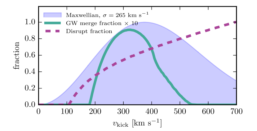
Figure 13: (Top) Possible post-kick orbital properties for a NS-BH binary formed from a low-metallicity system ($\log\leavevmode\nobreak\ Z=10^{-3.5}$) that passed through a ULX phase. The period and masses shown correspond to the pre-SN orbital parameters, and the kick distribution is taken to be a Maxwellian with a 1D rms of $\sigma=265\;{\rm km\;s^{-1}}$, and isotropic in space. After the kick, there is a $67\%$ chance that the binary is disrupted, and a $3.4\%$ chance that the resulting system is compact and eccentric enough to merge in a Hubble time. Solid lines indicate final orbital parameters for fixed kick velocity $v$ and variable angle $\theta$ formed between the kick velocity and the orbital velocity, assuming the kick to be on the orbital plane. Dashed lines indicate the same, except for a fixed $\theta$ and a variable $v$. The blue square at $P_{\rm orb}\simeq 27$ days and $e\simeq 0.07$ corresponds to a symmetric SN (i.e. no kick). (Bottom) Fraction of systems that would be disrupted or that would merge in less than a Hubble time for an isotropic fixed kick velocity.

Figure 13 shows the possible post-kick parameters when a NS is formed in a system of metallicity $\log\leavevmode\nobreak\ Z=-3.5$ with initial masses $M_{1}=70M_{\odot}$, $M_{2}=14M_{\odot}$ and an initial orbital period of $1.1$ days (illustrated in Figure 4). At core carbon depletion of the secondary it consists of a $55M_{\odot}$ BH and a $5.5M_{\odot}$ star with an orbital period of $23$ days. If there is no kick imparted on the NS, then the result is a NS-BH binary at a separation of $P_{\rm orb}\simeq 27$ days and a small eccentricity of $e\simeq 0.07$. Such a system would be too wide for GW radiation to have an important effect, with an expected merger time well in excess of $10000\leavevmode\nobreak\ \rm Gyr$. Still, detecting such a system while the NS is active as a pulsar would be very interesting, but considering a typical pulsar lifetime of $50\leavevmode\nobreak\ \rm Myr$, even if all ULXs would result in a NS-BH binary the expected number of observable sources would be low. As an upper bound, consider systems at a metallicity $\log\leavevmode\nobreak\ Z=-2.5$, for which we expect $2.6$ ULXs formed for every $10^{4}$ SNe. For a galaxy with a SNe rate of $0.01\leavevmode\nobreak\ \rm yr^{-1}$, this would mean $\sim 100$ NS-BH binaries with an active pulsar, which accounting for beaming, should result in less than $\sim 30$ observable pulsars. These would be extragalactic sources, making them hard to observe in radio, and as is shown in Figure 13, we would expect an important fraction to be disrupted from SNe kicks. However, the Square Kilometer Array will be capable of detecting pulsars beyond the large Magellanic clouds, and the discovery of a NS-BH binary is one of its key science goals (Kramer, 2004).

If the NS receives a kick of $\sim 200-500\leavevmode\nobreak\ \rm km\leavevmode\nobreak\ s^{-1}$ in a direction opposite to the orbital velocity, then the orbit can become very eccentric, with a merger time from GW radiation below a Hubble time. At lower kick velocities, despite the direction of the kick, the system cannot be driven to a large eccentricity, while for larger kicks the system would likely be disrupted. The system would circularize before entering the LIGO band, but if it is observed earlier in the LISA band, it could still retain a detectable eccentricity. As shown by Sesana (2016), GW150914 would have been detectable by LISA, and eccentricity measurements for sources at these high frequencies have been proposed as a way to distinguish between different formation scenarios for merging binary-BHs (Nishizawa et al., 2016; Breivik et al., 2016). This could also play a role in understanding the origin of NS-BH mergers.

For the system shown in Figure 13, there is a $3.4\%$ probability that it would merge in less than a Hubble time, and out of those $44\%$ would have merger times under $1\leavevmode\nobreak\ \rm Gyr$. The resulting inspiral would have a mass ratio $q=39$, and a BH with close to maximal spin. The spin and the mass ratio have opposite effects on the possibility of tidally disrupting the star and forming an accretion disk, with larger spins favoring tidal disruption. The simulations of Foucart (2012) show that at high mass ratios and low spins, the NS merges with the BH without being disrupted, producing no accretion disk and no electromagnetic counterpart. For systems at a mass ratio $q=10$ (the largest considered by Foucart, 2012) spin parameters above $a=0.8$ are required to produce an accretion disk, but even close to critical rotation, the disk might not be massive enough to power a strong EM signal. Owing to this, for the much higher mass ratios involved in our simulations, we would not expect the production of counterparts to a GW signal even if the BH is close to critical rotation. In the absence of an electromagnetic counterpart, it would be difficult to assess purely from a GW detection if the system contains a NS or if it is a BH-BH binary, since there is a strong degeneracy between mass-ratios and spins in parameter estimation (see, e.g. Hannam et al., 2013).

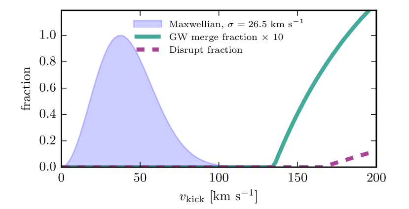
Figure 14: Same as Figure 13 but for a system where a BH would be expected to form from the secondary. We assume that $10\%$ of the stellar mass is lost during BH formation, and that the BH receives a kick with a 1D rms of $\sigma=26.5\;{\rm km\;s^{-1}}$. Kick velocities up to $v=135\rm km\leavevmode\nobreak\ s^{-1}$ are considered on the top panel, which corresponds to $99.999\%$ of the Maxwellian distribution.

A case where the secondary would form a BH is depicted in Figure 14. This system is the product of a binary with metallicity $\log\leavevmode\nobreak\ Z=-3.5$, initial masses $M_{1}=250M_{\odot}$ and $M_{2}=63M_{\odot}$ with an orbital period of $P_{\rm orb}=1.75$ days. The primary in this case forms a BH above the PISNe gap with a mass of $133M_{\odot}$, while the secondary reaches carbon depletion with a final mass of $36M_{\odot}$. Assuming a weak kick is imparted to the BH as described before, the chances of the system being disrupted are essentially zero, with $0.014\%$ of systems merging in less than a Hubble time formed from kick velocities at the tail of the Maxwellian distribution.

6.1 Rate estimates for NS-BH and BH-BH mergers

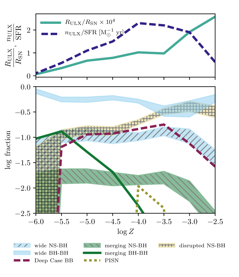
Figure 15: (Top) Production rate of ULXs in terms of the SN rate, and number of observable ULXs per $M_{\odot}\leavevmode\nobreak\ {\rm yr^{-1}}$ of SFR. (Bottom) Final outcomes after a ULX phase, represented as the fraction of the total of ULXs. Wide NS-BH and BH-BH systems correspond to binaries for which the merger time from GWs is longer than $13.8\leavevmode\nobreak\ \rm Gyrs$, while merging NS-BH and BH-BH systems are compact and/or eccentric enough to merge in less than that. Disrupted NS-BH systems correspond to binaries that were disrupted due to the kick imparted on the NS, while the number of disrupted BH-BH systems is negligible. Systems marked as Deep Case BB widen significantly due to mass transfer stripping hydrogen depleted layers of the donor, and we do not model them until core-carbon depletion. A small fraction of systems marked as PISN have secondaries massive enough to explode as PISNe, leaving only the BH produced by the primary. The values for NS-BH binaries, and for wide BH-BH binaries depend on the choice of threshold mass for BH formation.

Considering our full sample of ULX models, the different possible outcomes as a function of metallicity are shown in Figure 15. These values take into account the same distribution functions for the initial conditions as used in Section 4, and also consider possible uncertainties on the mass limit for BH formation by assuming a threshold of either $8M_{\odot}$ or $12M_{\odot}$ for final masses above which BHs are formed. At all metallicities considered the majority of systems would result in either wide BH-BH binaries or NS-BH systems that are disrupted due to the kick to the NS. The fraction that would result in a bound NS-BH binary is $\sim 10\%$, further reducing the chances of detecting such a system with an active pulsar. A similar fraction of systems undergo Case ABB/BB mass transfer driven by shell helium burning before carbon ignition, resulting in layers of hydrogen depleted material being stripped from the secondary. These stars are expected to lose most of their helium envelopes, resulting in stripped CO cores and, owing to the small final mass ratio, very wide binaries.

The most interesting possibility is the formation of NS-BH and BH-BH systems compact enough to merge from the emission of GWs in less than a Hubble time. For most of the metallicity range studied, $\sim 2\%$ of the ULXs would become a NS-BH binary compact enough to merge in a Hubble time, while for BH-BH binaries it is only at metallicities below $\log\leavevmode\nobreak\ Z=-4$ that a non-negligible number of sources could produce a merger. As the BH-BH rate is only relevant at extremely low metallicities and is strongly dependent on the strength of BH kicks which is not well understood, the numbers we provide for BH-BH mergers should be considered speculative. Table 2 shows the expected formation rates per SN for NS-BH and BH-BH compact enough to result in a merger, including the values weighted with the metallicity distribution of Langer & Norman (2006) at redshift $z=0$ to represent the local production rate.

$\log\leavevmode\nobreak\ Z$	$\displaystyle\frac{R_{\rm NS-BH}}{R_{\rm SN}}\times 10^{6}$	$\displaystyle\frac{R_{\rm BH-BH}}{R_{\rm SN}}\times 10^{6}$
$-2.5$	$0.33-0.91$	$0$
$-3.0$	$1.0-2.6$	$0$
$-3.5$	$1.2-2.1$	$0.076$
$-4.0$	$1.2-1.9$	$0.045$
$-4.5$	$0.87-1.6$	$0.16$
$-5.0$	$0.83-1.6$	$3.4$
$-5.5$	$0.41-0.80$	$4.4$
$-6.0$	$0-0.014$	$0.63$
local	0.069-0.18	0.00029

Table 2: Rate of production per SN of NS-BH and BH-BH systems formed after a ULX phase, which are compact enough to merge in less than a Hubble time. The NS-BH rate depends on the threshold mass at which a NS is formed, and the lower and upper bounds given correspond to assuming that for final core masses above $8M_{\odot}$ and $12M_{\odot}$ respectively BHs are formed instead of NSs.

The expected local formation rate is below one per million SNe for NS-BH mergers and below one per billion for BH-BH mergers, making this a very unlikely outcome of the evolution of massive stars .

To put this in the context of detectability by GW detectors, we can estimate a corresponding volumetric rate for the production of these objects. Taking a volumetric SNe rate of $1\times 10^{5}\leavevmode\nobreak\ \rm Gpc^{-3}yr^{-1}$ (see, e.g. Madau & Dickinson 2014) and using our upper bound for the local production rate of NS-BH binaries that would result in a merger, gives a very low rate of $0.018\leavevmode\nobreak\ \rm Gpc^{-3}\leavevmode\nobreak\ yr^{-1}$, which owing to the large fraction of short delay times these systems would have, is closely tracked by the rate of actual mergers. Even assuming a metallicity of $\log\leavevmode\nobreak\ Z=-3.5$ at which we get the largest formation rate, this would still give a very low upper boundary $<0.2\leavevmode\nobreak\ \rm Gpc^{-3}yr^{-1}$. These values are comparable to the lower end of the estimates from CE models (Abadie et al., 2010). At its third science run the LIGO detectors are expected to probe down to rates of $\sim 50\leavevmode\nobreak\ \rm Gpc^{-3}\leavevmode\nobreak\ yr^{-1}$ (Abbott et al., 2016b) for the merger of a $1.4M_{\odot}$ NS with a $10M_{\odot}$ BH, which is well above our estimated rate. The current generation of GW detectors is then unlikely to observe any of these mergers, but third generation detectors like the Einstein Telescope and the Big Bang Observatory, if operating at their expected sensitivities, should detect several of these events per year. Although the contribution of the CHE channel to the NS-BH merger rate might be sub-dominant, they would be characterized by very heavy BHs, with masses well in excess of $20M_{\odot}$.

7 Conclusions

In this work we have studied a new formation channel for ULXs. We find ULXs to form from massive very compact binaries with large mass ratios, where only the initially more massive star undergoes tidally induced chemically homogeneous evolution (CHE), and evolves into a massive BH without ever filling its Roche lobe. Thereafter, the less massive component expands and undergoes mass transfer to the more massive BH, often on the nuclear time scale (cf., Fig. 4). We explore this channel by computing large grids of detailed binary evolution models (see Appendix A), which allows us to fully characterize the ensuing ULX population (Appendix E). We summarize our main conclusions as follows:

1. At metallicities below $Z=0.01$, in binaries with initial orbital periods of $1\dots 3\,$d and mass ratios of $q\simeq 0.1-0.4$, primaries more massive than $45M_{\odot}$ may undergo CHE to form BHs of $20M_{\odot}$ or more. The secondary in these systems then expands and starts mass transfer to the BH. Assuming Eddington-limited accretion leads to mega-year long phases with X-ray luminosities in excess of $10^{40}\,$erg/s for many cases. This evolutionary path is expected to result in the most massive accreting stellar BHs possible at a given metallicity.

2. The occurrence of PISNe, which leave no compact remnant, leads to a gap in BH masses in the range $\sim 60M_{\odot}-130M_{\odot}$. At metallicities higher than $\log\leavevmode\nobreak\ Z=-3$ no BHs above the gap are expected, resulting in a cutoff in BH masses that might be observed as a cutoff in ULX luminosities. At lower metallicities, very massive stars are expected to form BHs above the PISN gap, potentially producing an observable gap in ULX luminosities (Fig. 8).

3. Locally, our new channel can account for the brightest observed ULXs, with $\sim 0.13$ sources per $M_{\odot}\leavevmode\nobreak\ \rm yr^{-1}$ of SFR. Observations of nearby galaxies give a rate of $2$ ULXs per $M_{\odot}\leavevmode\nobreak\ \rm yr^{-1}$ of SFR, so a different channel is required to explain the less luminous sources. The rate from our channel increases significantly in low metallicity environments, with a maximum of $2.3$ sources per $M_{\odot}\leavevmode\nobreak\ {\rm yr^{-1}}$ of SFR expected at a metallicity of $\log\leavevmode\nobreak\ Z=-4$.

4. The metallicity dependence of both the number and the luminosity of the ULXs predicted through our channel, implies that the ratio of the total X-ray luminosity of galaxies and the SFR increases significantly at extremely low metallicities.

5. The majority of our ULX binaries have orbital periods below $20\,$d and MS donors in the mass range $8M_{\odot}\dots 30M_{\odot}$, with a non-negligible number of donors up to $70M_{\odot}$, possibly explaining some bright optical counterparts to observed ULXs that are hard to explain with CE models. More than $90\%$ of our sources contain MS donors, transferring mass at rates below ten times $\dot{M}_{\rm Edd}$. ULXs formed through CHE are also expected to favor low mass ratios, with about $\sim 50\%$ of nearby sources having $q<0.5$.

6. After a ULX phase, depending on the mass of the donor, a NS-BH or BH-BH binary could be produced. There is a small but finite probability to produce NS-BH systems which are compact enough to merge in less than a Hubble time, with a formation rate of $<0.2\leavevmode\nobreak\ \rm Gpc^{-3}\leavevmode\nobreak\ yr^{-1}$. The detection of such mergers in the near future is not likely, but they would be characterized by having large mass ratios, with BHs more massive than $20M_{\odot}$.

Together with the results of (Marchant et al., 2016), who investigated similar binary systems to this study only focussing on mass ratios closer to one, we find that the tightest low-metallicity massive binaries may produce a wealth of exciting phenomena (Fig. 16). Since the primaries above $\sim 30M_{\odot}$ evolve chemically homogeneously (Fig. 2) due to tidal synchronisation, they do not expand and may produce BHs with a mass close to their initial mass. For mass ratios of $q\mathrel{\hbox{\hbox to0.0pt{\hbox{\lower 4.0pt\hbox{$\sim$}}\hss}\hbox{$>$}}}0.8$, the secondary may also follow CHE and form a second massive BH in the system, potentially leading to massive BH mergers. At lower mass ratios the secondaries follow ordinary evolution, leading to ULXs. In both cases, the mass range of BH formation is interrupted by the pair instability regime, leading to pair instability supernovae for primary masses roughly in the range $60M_{\odot}\dots 130M_{\odot}$. Finally, as rapid rotation is required for CHE, the BHs may form with high Kerr parameters, which may give rise to LGRBs within the framework of the collapsar model.

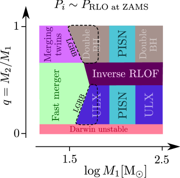
Figure 16: Schematic representation of the evolutionary end stages of massive low-metallicity binaries with the smallest possible initial orbital periods. See text for discussion.

Many of these outcomes can be assessed observationally in the coming years. We have argued that, at low metallicities, the distribution of X-ray luminosities of ULXs could present a pronounced gap, which upcoming missions such as eROSITA and Athena could possibly detect. A similar gap is expected in the distribution of chirp masses of merging double BHs (Marchant et al., 2016), which may be detectable by aLIGO at its design sensitivity. Current transient surveys such as the intermediate Palomar Transient Factory (Rau et al., 2009), the upcoming Zwicky Transient Facility (Bellm, 2014; Smith et al., 2014) and the Large-Synoptic-Survey telescope LSST (Tyson, 2002) may provide strong constraints on the existence and rates of PISNe. All these observations from very different instruments will provide strong tests of our models, and in particular of CHE in the closest massive binary systems.

Appendix A Grids of binary models

A summary of the outcomes of our simulations is presented in Figures 17-25. The meaning of the different labels in those figures is as follows:

• ZAMS L2OF: The initial orbital separation is so short that the system overflows the L2 Lagrangian point at ZAMS. Such a system should rapidly merge.

• ZAMS RLOF: System is undergoing RLOF at ZAMS. As shown in Marchant et al. (2016), these overcontact systems might survive interaction without merging, resulting in a binary with equal mass components. However, for low mass ratios we mostly expect the systems to evolve into deep contact and merge, and even for systems that avoid that, they would not follow the channel for ULX formation described in this work.

• off CHE: Primary reached a point where the difference between central and surface helium abundance is larger than $0.2$. We consider such systems are not evolving chemically homogeneous, and terminate these simulations.

• Case B/BB: The primary evolves chemically homogeneous and forms a BH. The secondary then initiates mass transfer and a possible ULX phase after depleting its central hydrogen. These systems are only expected to have a brief ULX phase. Some of these systems undergo an additional phase of case BB mass transfer after core helium depletion.

• Case AB/ABB: Similar to the previous one, only that mass transfer is initiated while the secondary is on the MS so it operates on a much longer nuclear timescale.

• PISN: The final mass of the primary at helium depletion is in the range $60<M_{1,\rm f}<130$, so we expect to result in a SN leaving the secondary as a single star.

• no MT (double BH): Both stars evolve chemically homogeneous, avoiding mass transfer and resulting in a compact binary BH. This is the path of evolution discussed in Marchant et al. (2016). For the mass ratios studied, only a handful of these systems are found.

• MT before BH forms: Mass transfer, either from the primary or the secondary, happens before BH formation. We expect such systems to either merge (in case the primary is the donor) or widen and interrupt CHE because of accretion of hydrogen-rich material (if the secondary is the donor), which would not result in the formation of a ULX.

• convergence error: Due to numerical problems the simulation was not completed.

• Darwin unstable: At its initial state the system has an orbital separation smaller than $a_{Darwin}$, and thus is Darwin unstable. It would not be possible to form a synchronized binary with this orbital separation, as it would result in a merger instead. The moment of inertia is dependent in the initial rotation rate, which results in some irregularities in the boundary between stable and unstable models.

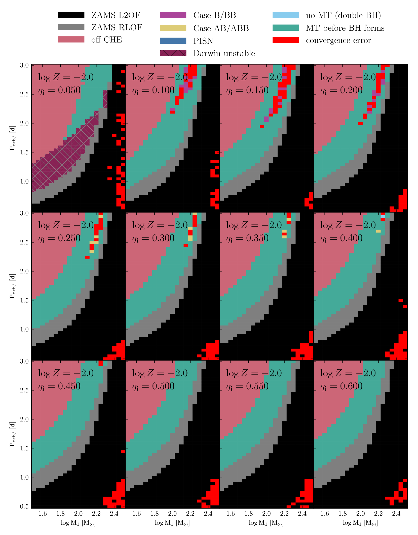
Figure 17: Grid of models for $\log Z=-2.0$. See text in Appendix A for an explanation.

Figure 18: Grid of models for $\log Z=-2.5$. See text in Appendix A for an explanation.

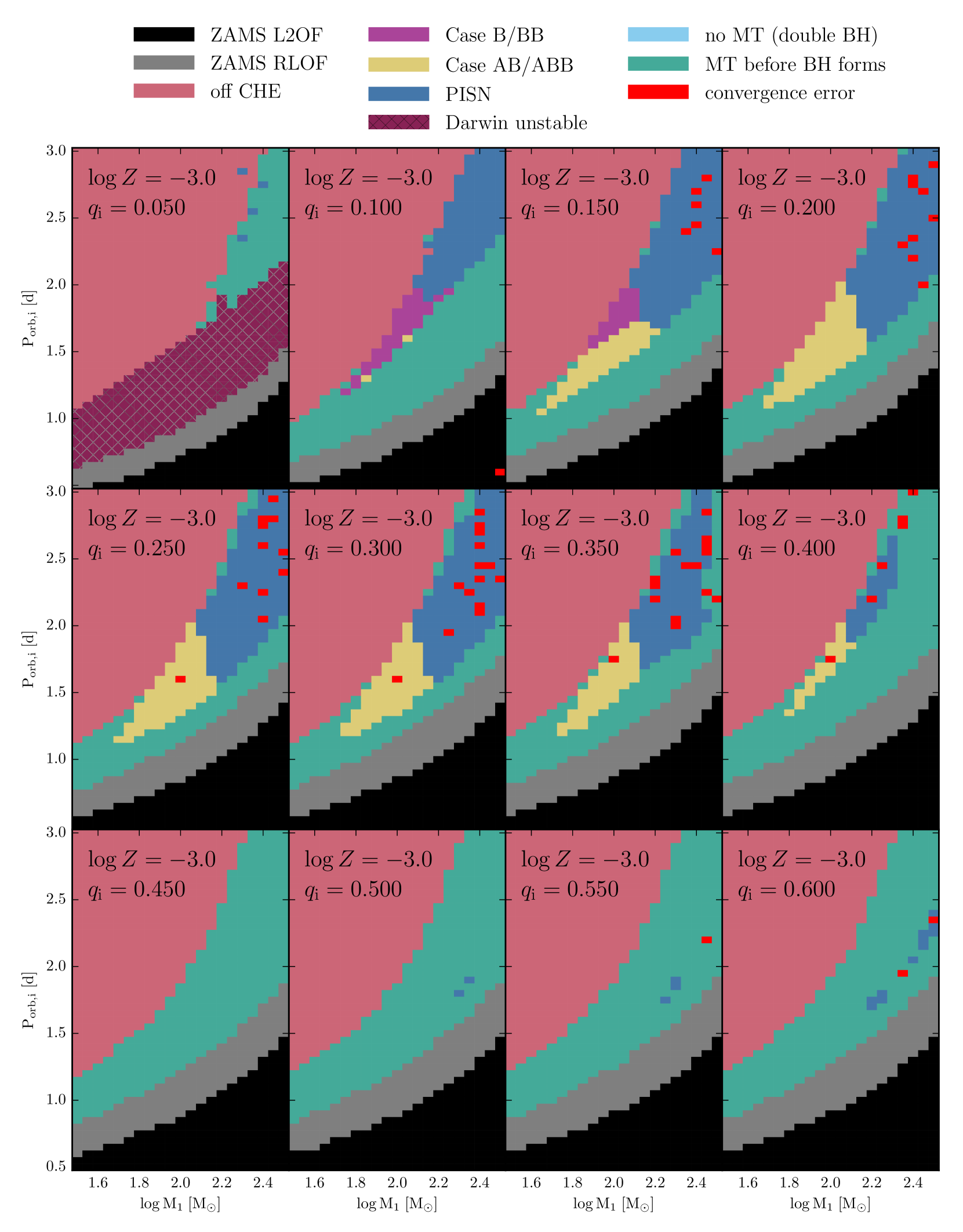
Figure 19: Grid of models for $\log Z=-3.0$. See text in Appendix A for an explanation.

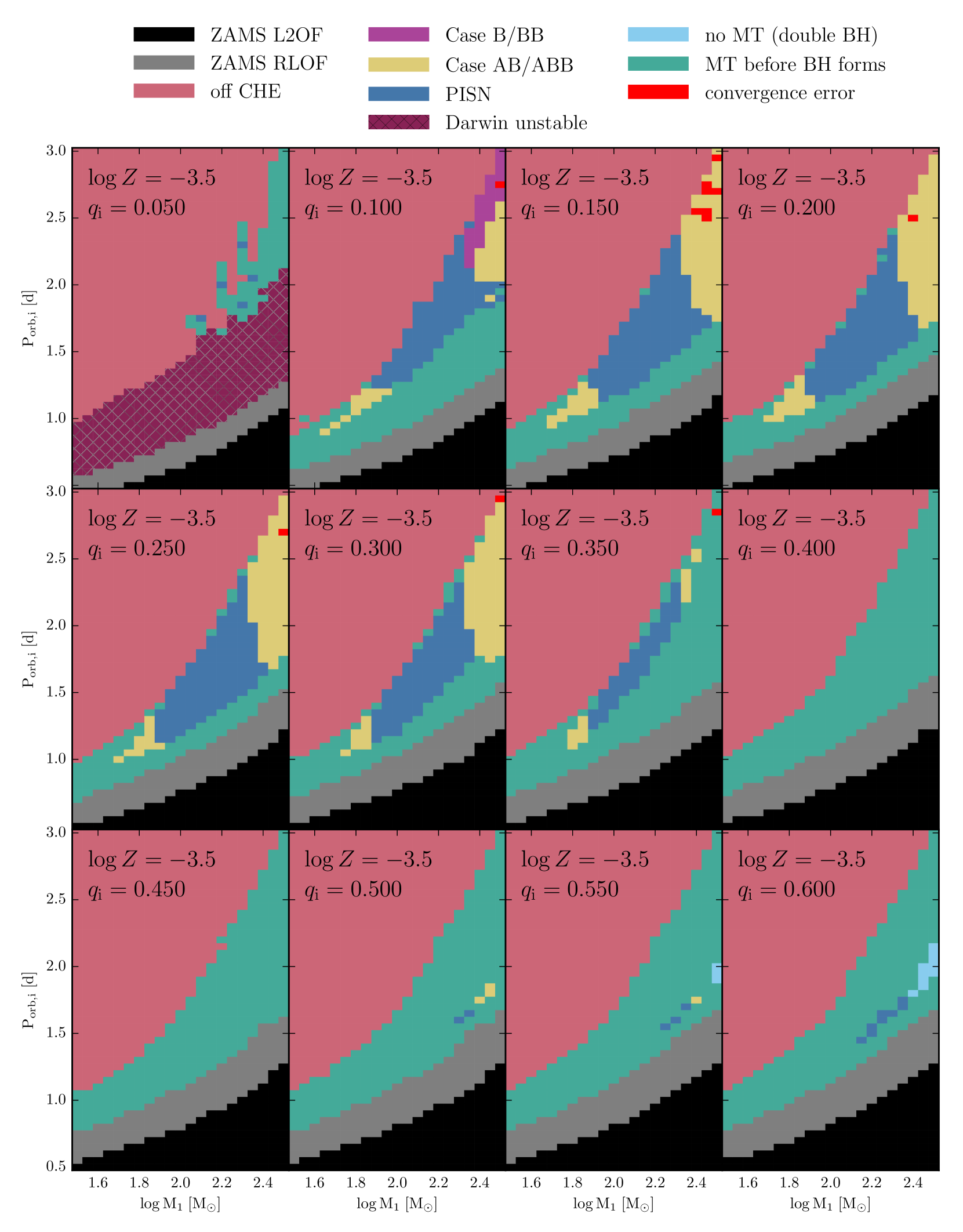
Figure 20: Grid of models for $\log Z=-3.5$. See text in Appendix A for an explanation.

Figure 21: Grid of models for $\log Z=-4.0$. See text in Appendix A for an explanation.

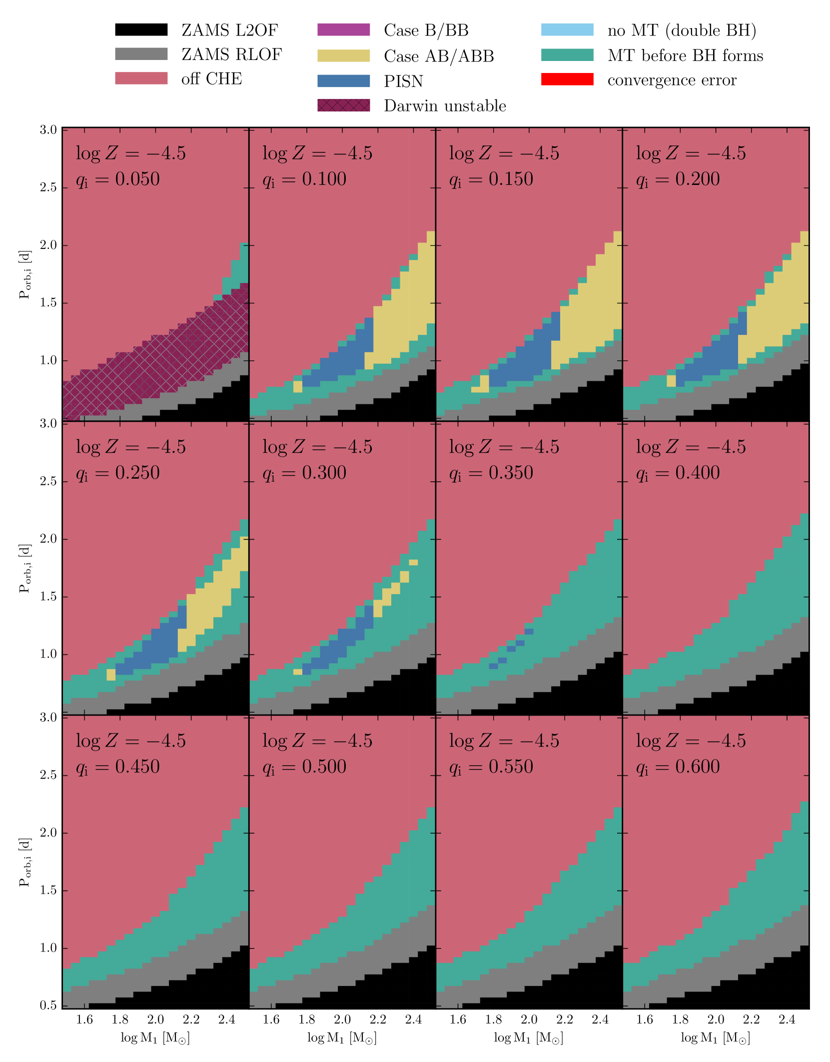
Figure 22: Grid of models for $\log Z=-4.5$. See text in Appendix A for an explanation.

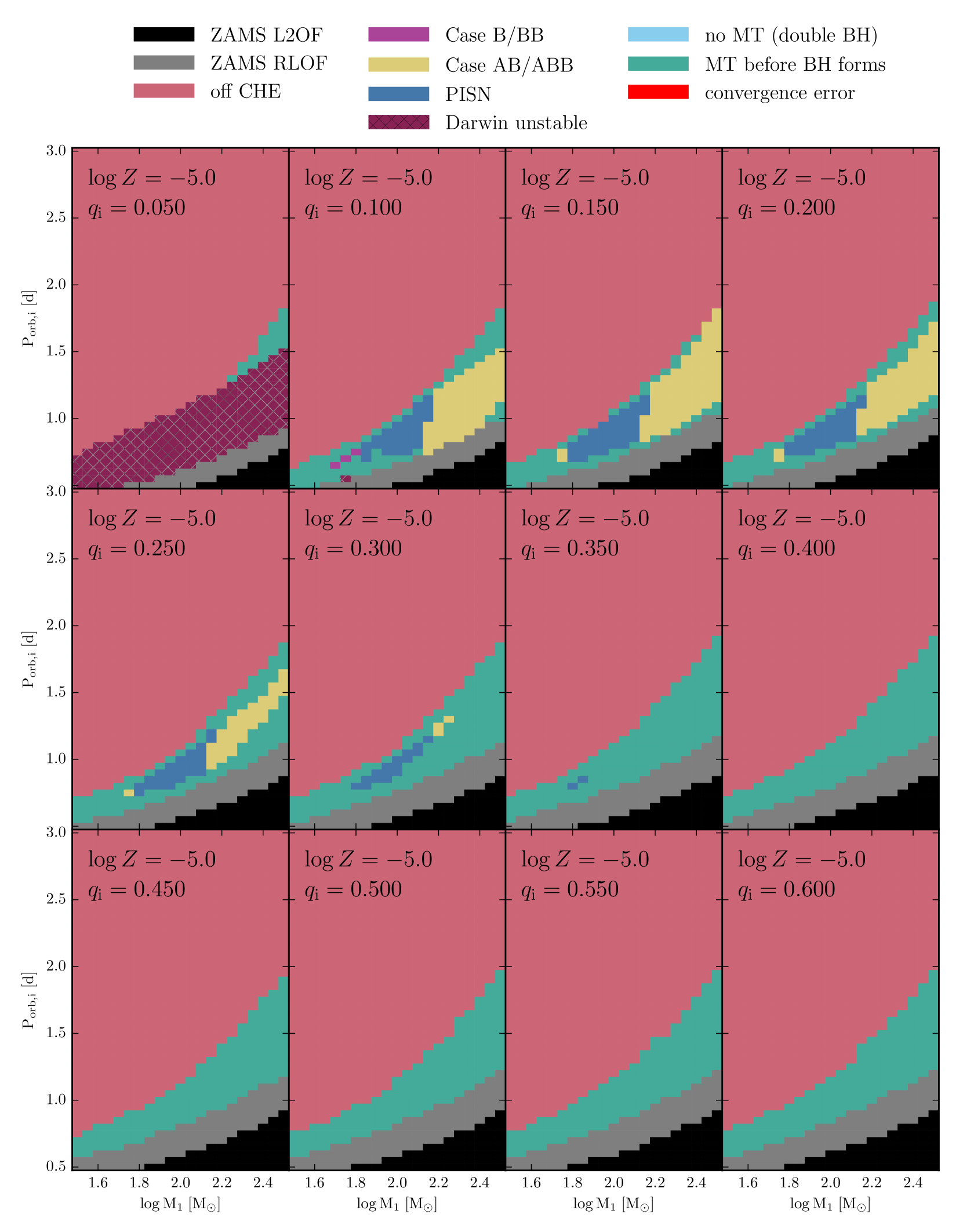
Figure 23: Grid of models for $\log Z=-5.0$. See text in Appendix A for an explanation.

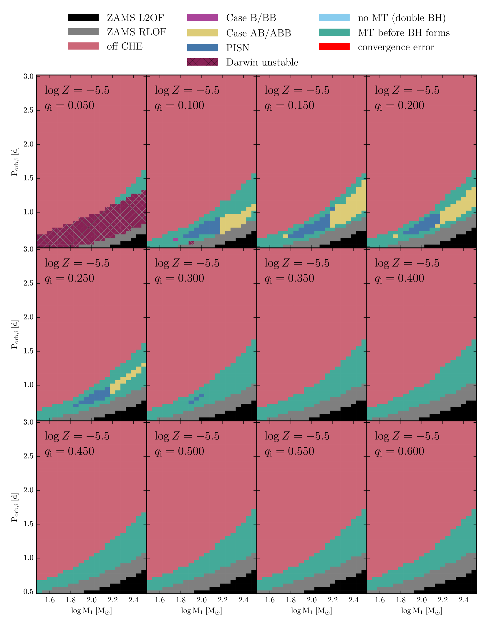
Figure 24: Grid of models for $\log Z=-5.5$. See text in Appendix A for an explanation.

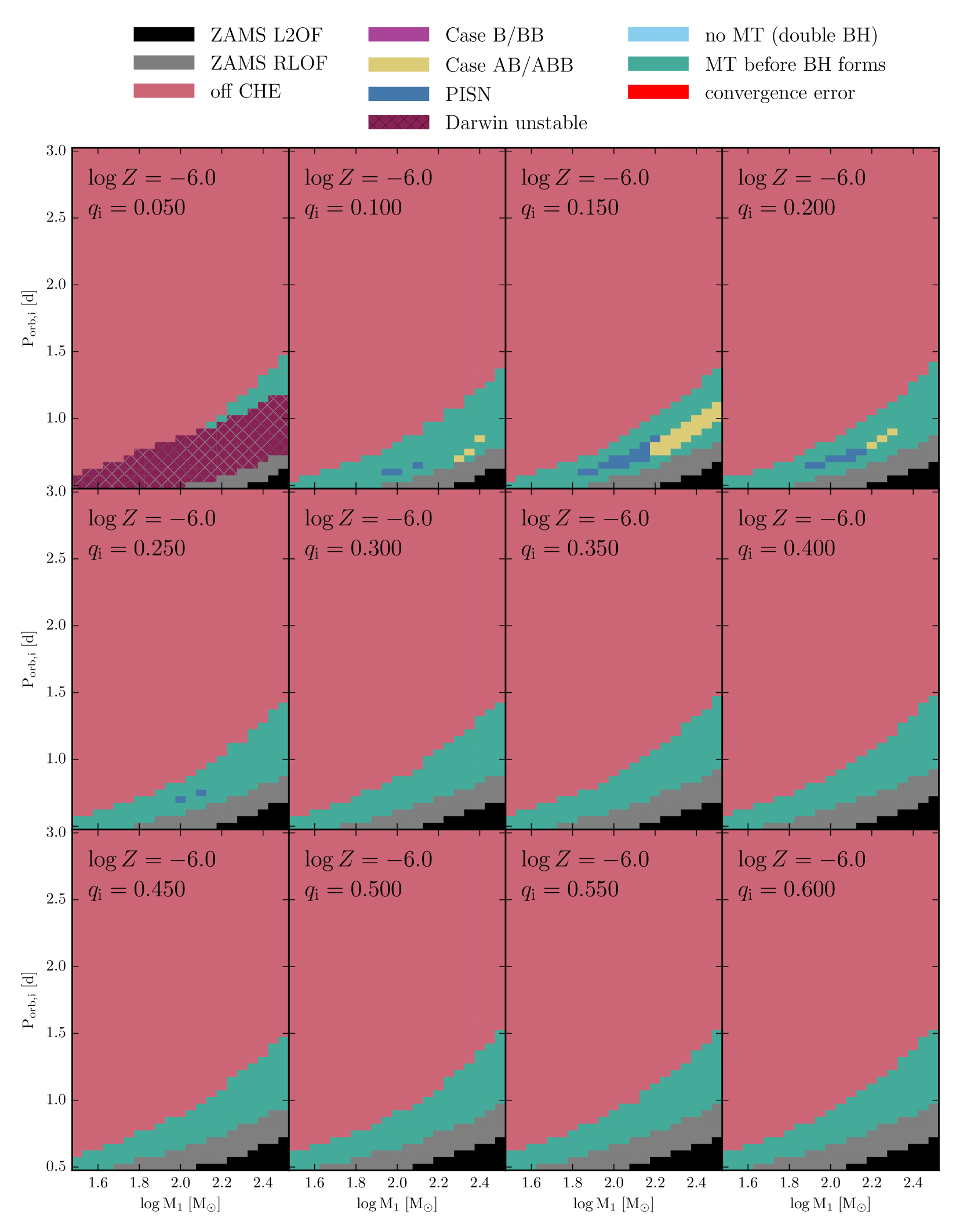
Figure 25: Grid of models for $\log Z=-6.0$. See text in Appendix A for an explanation.

Appendix B Computation of the formation rate and number of observable ULXs

To compute the number of ULXs formed per core-collapse SN, we first consider the binary fraction $f_{\rm b}$ defined as the ratio between the number of binary systems formed to the total number of binaries and singles formed. Our assumption that out of three massive stars two are formed in a binary implies $f_{\rm b}=0.5$. We further assume that the lower mass threshold for a single star to result in a SN is $M_{\rm SN}=8M_{\odot}$, and that binaries containing primaries with masses $M_{1}>M_{\rm SN}$ produce two SNe. Using this, the formation rate of massive binaries $R_{\rm MB}$, defined as the number of binaries with primary masses above $M_{\rm SN}$ formed per unit time in a given galaxy (or collection of galaxies), can be related to the formation rate of SNe of that galaxy, $R_{\rm SN}$:

$$R_{\rm MB}=\frac{f_{\rm b}}{1+f_{\rm b}}R_{\rm SN}.$$ (10)

Taking into account the results of our binary models, we can define a function $F_{\rm ULX}(M_{\rm 1,i},q_{\rm i},P_{\rm i},Z)$ which is either $1$ or $0$ depending on whether a binary system with the corresponding initial parameters results in a ULX or not. Considering a distribution of initial binary parameters given by

$$\frac{dN}{dM_{1,\rm i}}\propto f_{M}(M_{1,\rm i}),\quad\frac{dN}{dq}\propto f_{q}(q),\quad\frac{dN}{dP_{\rm i}}\propto f_{P}(P_{\rm i}),$$ (11)

the rate of formation of ULXs can be expressed in terms of the SN rate as

$$\begin{aligned} \frac{R_{\rm ULX}}{R_{\rm SN}}=\frac{f_{\rm b}}{1+f_{\rm b}}\times\qquad\qquad\qquad\qquad\qquad\qquad\qquad\qquad\\ \qquad\qquad\frac{\displaystyle\int_{M_{\rm SN}}^{\infty}\int_{0}^{1}\int_{P_{\rm min}}^{P_{\rm max}}F_{\rm ULX}f_{M}f_{q}f_{P}\;dP_{\rm i}dq_{\rm i}dM_{1,\rm i}}{\displaystyle\int_{M_{\rm SN}}^{\infty}\int_{0}^{1}\int_{P_{\rm min}}^{P_{\rm max}}f_{M}f_{q}f_{P}\;dP_{\rm i}dq_{\rm i}dM_{1,\rm i}}.\end{aligned}$$ (12)

To compute the number of observable ULXs in a galaxy, $n_{\rm ULX}$, we need to take into account the duration of a ULX phase, which we define as $t_{\rm ULX}(M_{\rm 1,i},q_{\rm i},P_{\rm i},Z)$. Furthermore, if we assume the formation rate of SNe is proportional to the $\rm SFR$, $n_{\rm ULX}$ is then given by

$$\begin{aligned} \frac{n_{\rm ULX}}{\rm SFR}=\frac{f_{\rm b}}{1+f_{\rm b}}\frac{R_{\rm SN}}{\rm SFR}\times\qquad\qquad\qquad\qquad\qquad\qquad\qquad\\ \qquad\qquad\frac{\displaystyle\int_{M_{\rm SN}}^{\infty}\int_{0}^{1}\int_{P_{\rm min}}^{P_{\rm max}}t_{\rm ULX}f_{M}f_{q}f_{P}\;dP_{\rm i}dq_{\rm i}dM_{1,\rm i}}{\displaystyle\int_{M_{\rm SN}}^{\infty}\int_{0}^{1}\int_{P_{\rm min}}^{P_{\rm max}}f_{M}f_{q}f_{P}\;dP_{\rm i}dq_{\rm i}dM_{1,\rm i}},\end{aligned}$$ (13)

and for this work we have used $R_{\rm SN}/{\rm SFR}=0.01\;M_{\odot}^{-1}$. For a different value of this ratio, all results presented in this paper can easily be scaled. Finally, the average time that systems resulting in a ULX spend as active sources can be computed as

$$\begin{aligned} \langle t_{\rm ULX}\rangle=\frac{n_{\rm ULX}}{R_{\rm ULX}}=\qquad\qquad\qquad\qquad\qquad\qquad\qquad\qquad\\ \qquad\qquad\frac{\displaystyle\int_{M_{\rm SN}}^{\infty}\int_{0}^{1}\int_{P_{\rm min}}^{P_{\rm max}}t_{\rm ULX}f_{M}f_{q}f_{P}\;dP_{\rm i}dq_{\rm i}dM_{1,\rm i}}{\displaystyle\int_{M_{\rm SN}}^{\infty}\int_{0}^{1}\int_{P_{\rm min}}^{P_{\rm max}}F_{\rm ULX}f_{M}f_{q}f_{P}\;dP_{\rm i}dq_{\rm i}dM_{1,\rm i}}.\end{aligned}$$ (14)

Appendix C Evolution of models accreting above $\dot{M}_{\rm Edd}$

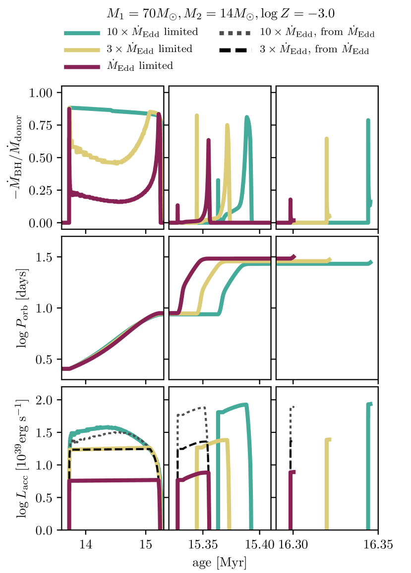
Figure 26: Zoom-in into the three mass transfer phases of the ULX model at metallicity $\log Z=-3.0$ shown in Figure 7, including simulations where the Eddington limit was increased by factors of $3$ and $10$. Dashed and dotted lines show the estimated luminosity that simulations with increased Eddington factors would have, using the potential luminosity a source could reach in the simulation strictly limited to the Eddington rate. (top) Mass transfer efficiency. (middle) Orbital periods. (bottom) Accretion luminosity.

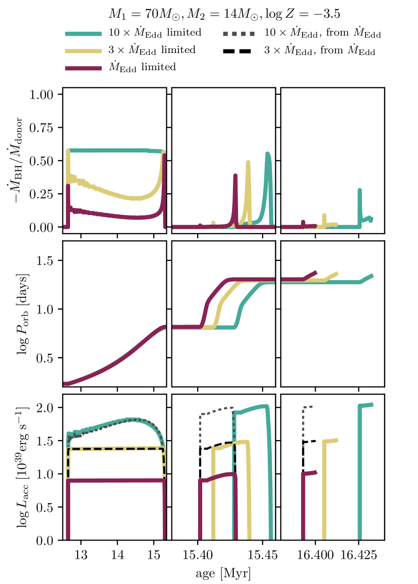
Figure 27: Same as figure 26, bur for a metallicity $\log Z=-3.5$

In section 4 we consider how the distribution of ULX luminosities varies if the BH can accrete either at three or ten times its Eddington rate. This is not done self-consistently, but rather by post-processing our simulation grids that are strictly limited to the Eddington rate, and considering the potential luminosity they could reach at different phases. Figures 26 and 27 show two examples of this, comparing the estimated luminosities with simulations where the Eddington limit is increased self-consistently.

The longer lasting X-ray phase, which is expected to dominate in observed populations, is Case A mass transfer, which is depicted on the left panels of Figures 26 and 27. When accreting at 10 times the Eddinton rate, for both metallicites shown, Case A mass transfer becomes as efficient as it can be, while not becoming completely conservative due to wind mass loss from the donor and the loss of a significant amount of accreted mass as radiation (see Equation 4). Despite the change in efficiency, the evolution of the orbital periods remains more or less the same, as the final mass ratios are very similar, and the evolution of orbital angular momentum is dominated by wind mass loss of the donor and spin-orbit coupling, which are not modified by the efficiency of accretion. For both metallicites, the non-self-consistent method does a very good job in reproducing both the luminosities and lifetimes of ULX phases.

For the post main-sequence mass-transfer phases shown in the middle and right panels of Figures 26 and 27, mass-transfer rates are about two orders of magnitude above the Eddington limit, such that all models considered accrete inefficiently, even when allowed to do so at ten times the Eddington rate. The resulting orbital evolution is then almost identical, with luminosities and lifetimes of ULXs in models with increased Eddington rates being well reproduced from the model strictly limited to $\dot{M}_{\rm Edd}$.

Appendix D Construction of synthetic galaxies at a fixed SFR

To model the X-ray luminosities that individual galaxies would have for a given SFR, we consider all individual timesteps for each binary model simulated at a given metallicity, and account for the probability of each of these to be observed. In the following, we consider a timestep of size $\Delta t$ at a given point in time for a simulation with initial parameters $M_{1,\rm i}$, $q_{\rm i}$, $P_{\rm i}$ and $Z$, during which the binary is predicted to be an X-ray source with luminosity $L_{\rm X}$. The rate at which such a system would form is independent of $\Delta t$, and can be computed in terms of the SFR as

$$\begin{aligned} \frac{R_{\rm\Delta t}}{\rm SFR}=\frac{f_{\rm b}}{1+f_{\rm b}}\frac{R_{\rm SN}}{\rm SFR}\times\qquad\qquad\qquad\qquad\qquad\qquad\qquad\\ \qquad\qquad\frac{\displaystyle f_{M}f_{q}f_{P}\;\Delta P_{\rm i}\Delta q_{\rm i}\Delta M_{1,\rm i}}{\displaystyle\int_{M_{\rm SN}}^{\infty}\int_{0}^{1}\int_{P_{\rm min}}^{P_{\rm max}}f_{M}f_{q}f_{P}\;dP_{\rm i}dq_{\rm i}dM_{1,\rm i}},\end{aligned}$$ (15)

where $\Delta P_{\rm i}$, $\Delta q_{\rm i}$ and $\Delta M_{1,\rm i}$ are the spacings in the parameter space of our simulation grids corresponding to the particular model in question. The probability of observing $k$ such systems in a galaxy can can then be determined using a Poisson distribution,

$$P(k)=\frac{\lambda^{k}e^{-\lambda}}{k!},\quad\lambda=R_{\Delta t}\Delta t.$$ (16)

A synthetic galaxy can then be constructed by sampling this probability distribution for each timestep in all simulations at a given metallicity, and adding up the individual contributions of $kL_{\rm X}$ to the total X-ray luminosity of the galaxy, $L_{\rm X,gal}$.

The average ratio between galactic X-ray luminosities and SFRs can be computed without the need to model a large population as

$$\begin{aligned} \left\langle\frac{L_{\rm X,\rm gal}}{\rm SFR}\right\rangle=\frac{f_{\rm b}}{1+f_{\rm b}}\frac{R_{\rm SN}}{\rm SFR}\times\qquad\qquad\qquad\qquad\qquad\qquad\qquad\\ \qquad\quad\frac{\displaystyle\int_{M_{\rm SN}}^{\infty}\int_{0}^{1}\int_{P_{\rm min}}^{P_{\rm max}}\int_{0}^{t_{\rm f}}L_{\rm X}(t)f_{M}f_{q}f_{P}\;dt\,dP_{\rm i}dq_{\rm i}dM_{1,\rm i}}{\displaystyle\int_{M_{\rm SN}}^{\infty}\int_{0}^{1}\int_{P_{\rm min}}^{P_{\rm max}}f_{M}f_{q}f_{P}\;dP_{\rm i}dq_{\rm i}dM_{1,\rm i}},\end{aligned}$$ (17)

where we integrate over the age $t$ of a binary with given initial parameters, from the ZAMS to the endpoint of its evolution, $t_{\rm f}$. We have verified that our synthetic galactic models satisfy this average, which can also be seen from the models at high values of SFR in Figure 11 following the expected linear trend.

Appendix E Properties of ULXs

Figures 28-35 show several properties of our ULX models, including BH masses, accretion luminosities assuming mass transfer is limited to the Eddington rate, BH spins, the ratio between mass transfer and the Eddington rate $\dot{M}_{\rm mt}/\dot{M}_{\rm Edd}$, donor masses, and orbital periods. Color plots indicate in logarithmic scale 2D density distributions of all quantities against BH masses, while histograms are in a linear scale. For all metallicities, we use the distributions described in Section 4 for the mass of the primary, the mass ratio, and the orbital separation of the binary. These distributions take into account the lifetimes of different phases, and so correspond to the observable distributions at a fixed metallicity.

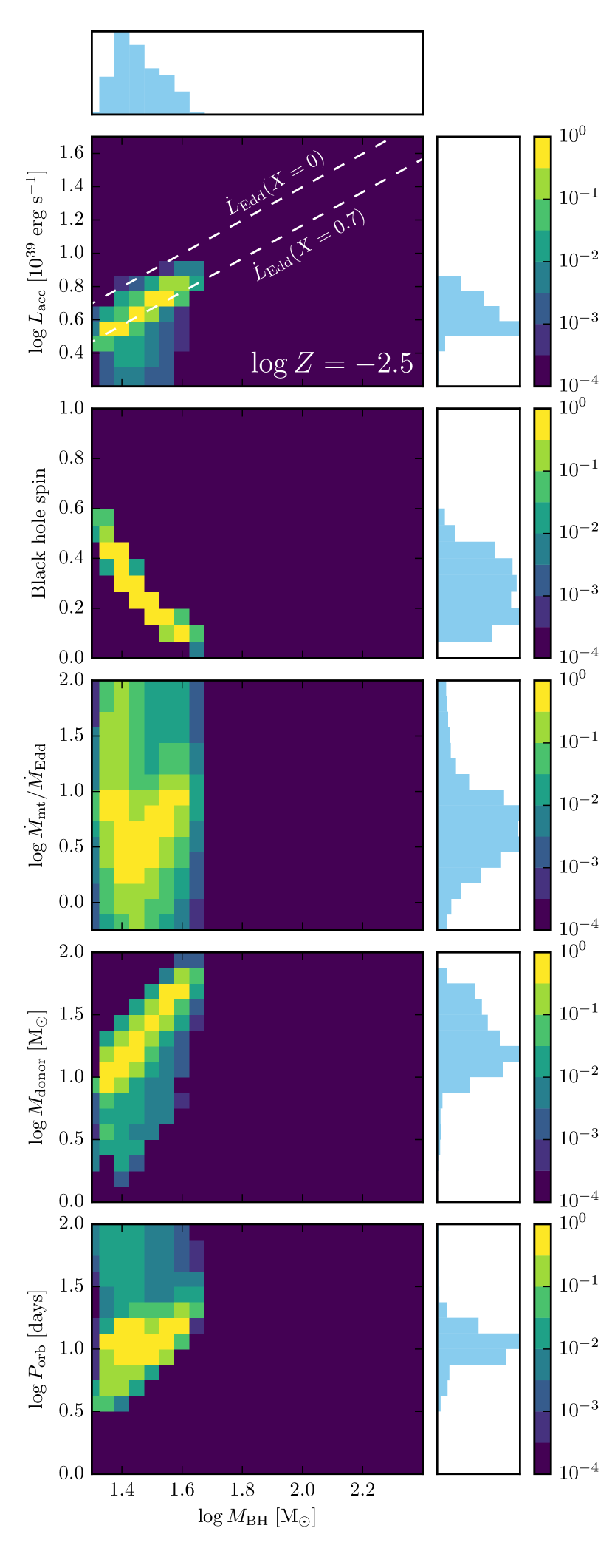
Figure 28: General properties of ULXs for $\log Z=-3.0$. See text in Appendix E for an explanation.

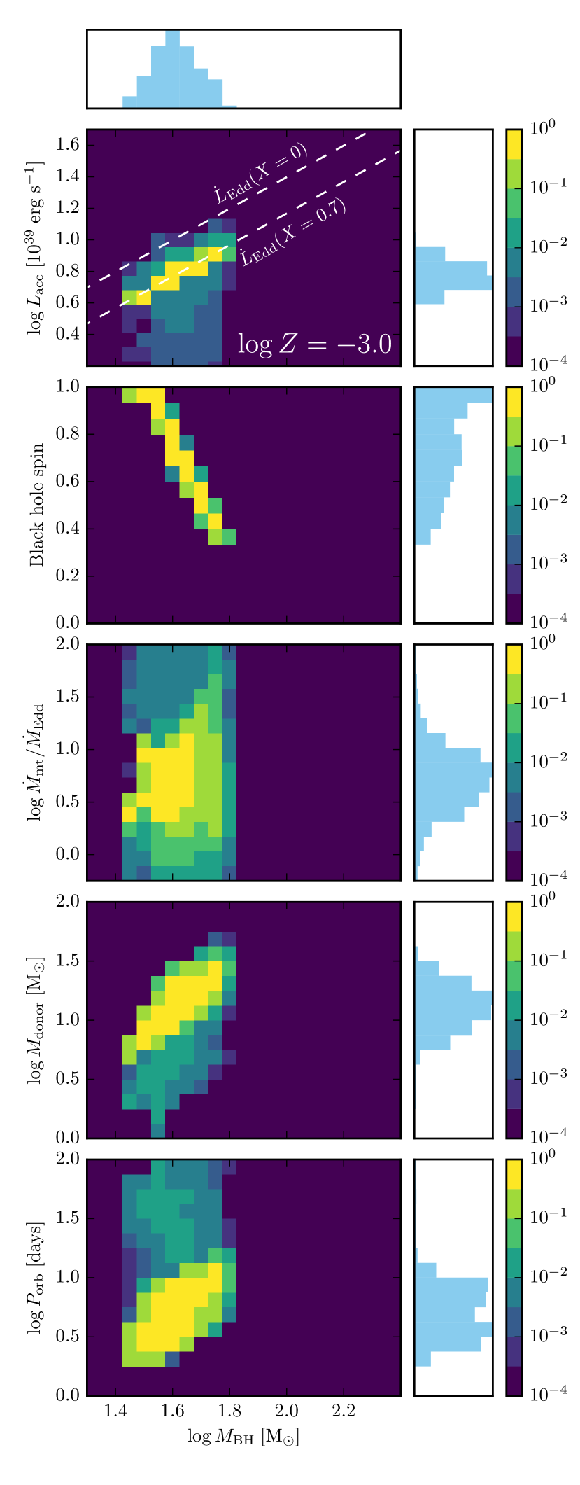
Figure 29: General properties of ULXs for $\log Z=-3.0$. See text in Appendix E for an explanation.

Figure 30: General properties of ULXs for $\log Z=-3.0$. See text in Appendix E for an explanation.

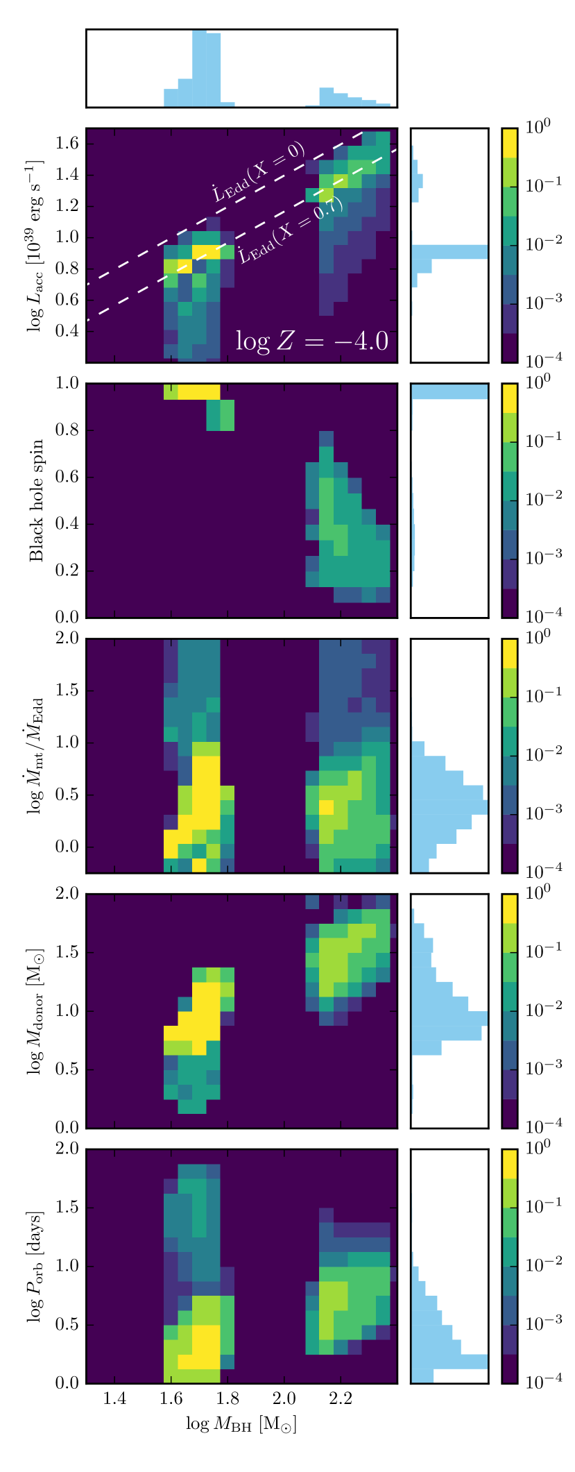
Figure 31: General properties of ULXs for $\log Z=-4.0$. See text in Appendix E for an explanation.

Figure 32: General properties of ULXs for $\log Z=-4.5$. See text in Appendix E for an explanation.

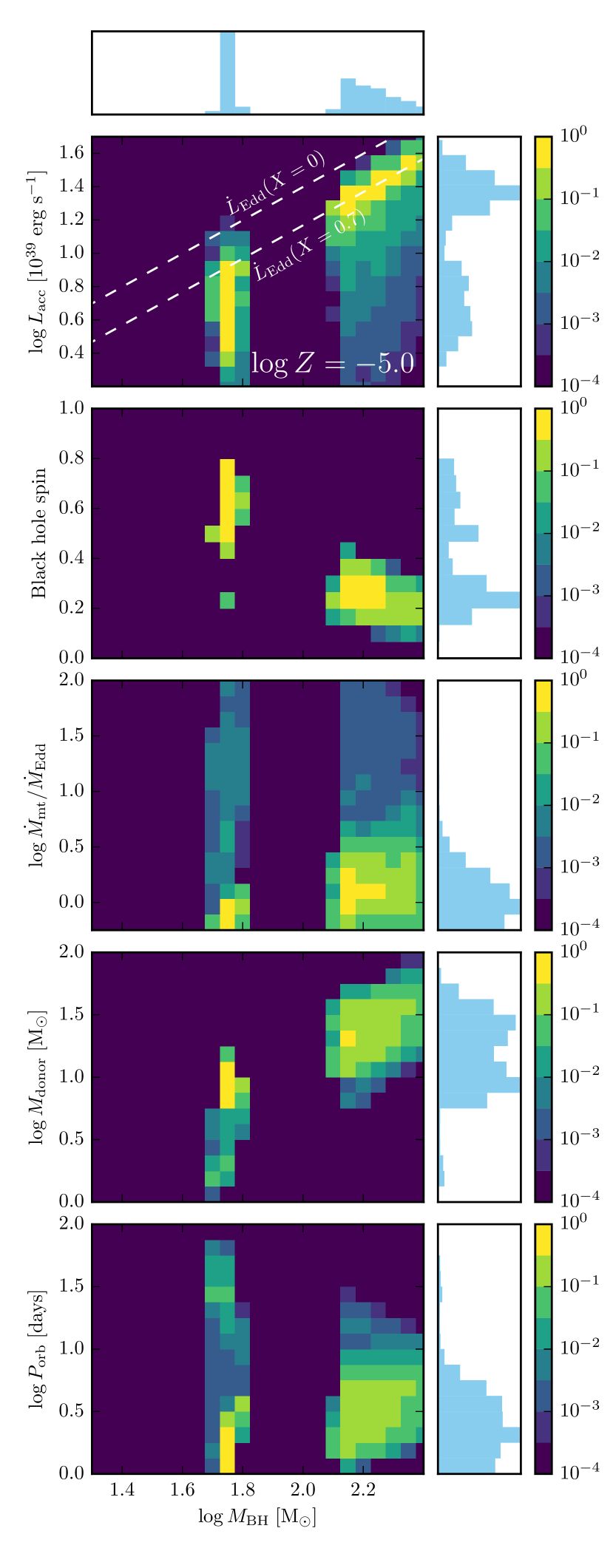
Figure 33: General properties of ULXs for $\log Z=-5.0$. See text in Appendix E for an explanation.

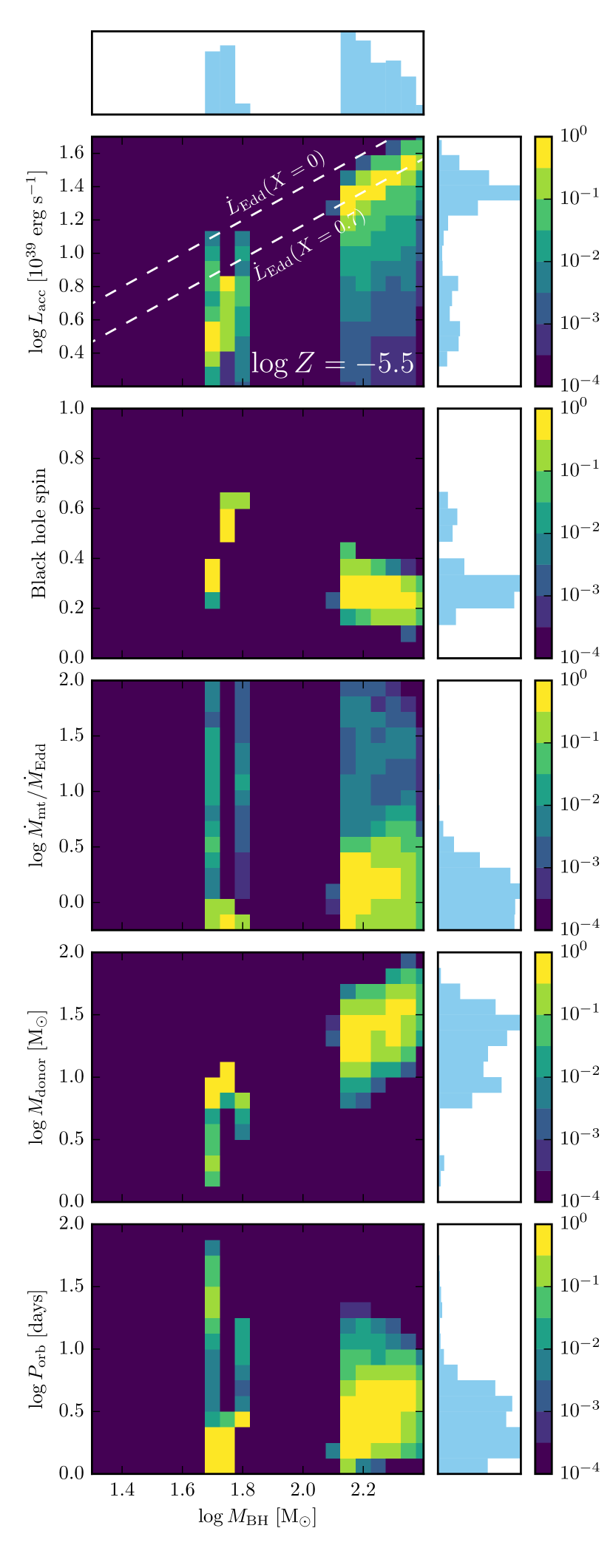
Figure 34: General properties of ULXs for $\log Z=-5.5$. See text in Appendix E for an explanation.

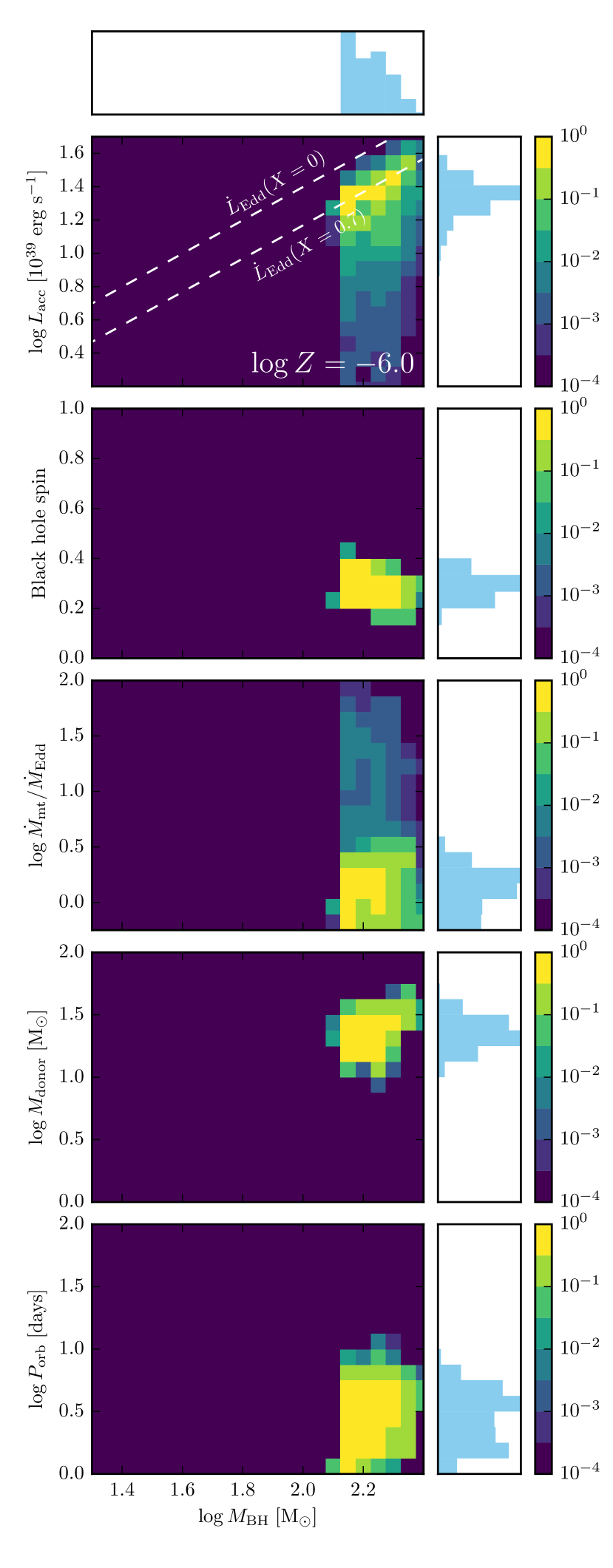
Figure 35: General properties of ULXs for $\log Z=-6.0$. See text in Appendix E for an explanation.