Dynamical tides in coalescing superfluid neutron star binaries with hyperon cores and their detectability with third generation gravitational-wave detectors

Abstract

The dynamical tide in a coalescing neutron star binary induces phase shifts in the gravitational waveform as the orbit sweeps through resonances with individual g-modes. Unlike the phase shift due to the equilibrium tide, the phase shifts due to the dynamical tide are sensitive to the stratification, composition, and superfluid state of the core. We extend our previous study of the dynamical tide in superfluid neutron stars by allowing for hyperons in the core. Hyperon gradients give rise to a new type of composition g-mode. Compared to g-modes due to muon-to-electron gradients, those due to hyperon gradients are concentrated much deeper in the core and therefore probe higher density regions. We find that the phase shifts due to resonantly excited hyperonic modes are $\sim$$10^{-3}\textrm{ rad}$, an order of magnitude smaller than those due to muonic modes. We show that by stacking events, third generation gravitational-wave detectors should be able to detect the phase shifts due to muonic modes. Those due to hyperonic modes will, however, be difficult to detect due to their smaller magnitude.

1 Introduction

Tides in coalescing neutron star (NS) binaries modify the rate of inspiral and generate phase shifts in the gravitational wave (GW) signal that encode information about the the NS interior. The tide is often decomposed into an equilibrium tide and a dynamical tide, where the former represents the fluid’s quasi-static response and the latter represents its resonant response (e.g., in the form of resonantly excited g-modes). The GW phase shift due to the equilibrium tide, which should be detectable with Advanced LIGO (LIGO Scientific Collaboration et al., 2015) by stacking multiple merger events, can constrain the NS tidal deformability and therefore the supranuclear equation of state (Read et al., 2009; Hinderer et al., 2010; Damour et al., 2012; Del Pozzo et al., 2013; Lackey & Wade, 2015; Agathos et al., 2015). However, the equilibrium tide can only indirectly constrain the interior stratification (i.e., the composition profile; Chatziioannou et al. 2015) and is insensitive to superfluid effects (see, e.g., Penner et al. 2011). By contrast, the dynamical tide is directly sensitive to both the stratification (Shibata, 1994; Lai, 1994; Reisenegger & Goldreich, 1994; Kokkotas & Schafer, 1995; Ho & Lai, 1999; Hinderer et al., 2016; Steinhoff et al., 2016) and superfluid effects (Yu & Weinberg, 2017). GW phase shifts due to the dynamical tide can therefore provide a unique probe of the NS interior, similar to asteroseismology observations which are now providing detailed constraints on the physics of the interiors of white dwarfs, solar-type stars, and red giants (Winget & Kepler, 2008; Chaplin & Miglio, 2013).

Previous studies of the dynamical tide in binary NSs focused on ‘canonical’ $1.4M_{\odot}$ NSs and assumed that the core does not contain exotic hadronic matter, such as hyperons. Although it is energetically favorable for nuclear matter to transition to hyperonic matter at high densities (Ambartsumyan & Saakyan, 1960), the discovery of $2M_{\odot}$ NSs (Demorest et al., 2010; Antoniadis et al., 2013) ruled out many hyperonic models since they tend to have softer equations of state. However, the degree of softening is uncertain (Lonardoni et al., 2015) and in the last few years many new hyperonic models compatible with the observations of $2M_{\odot}$ NSs have been proposed (e.g., Bednarek et al. 2012; Weissenborn et al. 2012; Gusakov et al. 2014; Tolos et al. 2016).

The dynamical tide in hyperonic models is modified by the hyperon composition gradient, which provides a new source of buoyancy that can support g-mode oscillations much deeper within the NS core than the leptonic composition gradient (Dommes & Gusakov, 2016). GW phase shifts induced by the excitation of hyperonic g-modes therefore probe the innermost core, where the density is a few times the nuclear saturation density.

The total phase shift accumulated over the inspiral due to the equilibrium tide is $\sim 1\textrm{ rad}$ while that due to the dynamical tide is only $\lesssim 10^{-2}\textrm{ rad}$. However, their detectability is not as different as these numbers might suggest. In part, this is because the dynamical tide phase shift accumulates at lower GW frequencies, where ground-based detectors are more sensitive. There is also more time before the merger to build up the signal-to-noise ratio (SNR) and compare the waveform signal before and after resonance. In addition, because the dynamical tide causes small but sudden increases in GW frequency at mode resonances, it has a unique signature that cannot be easily mimicked by varying other parameters of the binary (such as the masses).

In this paper we extend our previous study of dynamical tides in superfluid NSs (Yu & Weinberg, 2017) in order to account for the possible presence of hyperons in the core. We also evaluate the detectability of the phase shifts induced by the dynamical tide with second and third generation GW detectors. We begin in Section 2 by describing our background hyperonic NS model and in Section 3 we solve for its g-modes. In Section 4, we consider the resonant tidal driving of the g-modes and calculate the resulting GW phase shift. In Section 5, we evaluate the prospects for detecting the phase shifts with current and future GW detectors.

2 SUPERFLUID MODELS with hyperons

We construct our background superfluid models using an approach similar to that of Yu & Weinberg (2017; hereafter YW17), but with some key differences described below; we refer the reader to YW17 and references therein for further details, particularly as pertains to our treatment of the thermodynamics. Briefly, we assume that the background star is non-rotating, cold (zero temperature), in chemical equilibrium, and that all charge densities are balanced. We treat the neutrons in the core as superfluid and all other particle species (protons, $\Lambda$-hyperons, electrons, and muons) as normal fluid matter.

The two main differences between the present approach and that of YW17 are that here: (1) we use the GM1’B equation of state (Gusakov et al., 2014) rather than SLy4(Rikovska Stone et al., 2003), and (2) we solve the general relativistic (GR) Tolman-Oppenheimer-Volkhov (TOV) equations of stellar structure rather than the Newtonian equations. We use GM1’B because it allows for the existence of hyperons in the inner core, is consistent with the existence of $2M_{\odot}$ NSs, and Gusakov et al. (2014) provide enough detail to allow for a calculation of the Brunt-Väisälä frequency, $\mathcal{N}$, and thus g-modes. Regarding the second point, in YW17 we solved the Newtonian equations of stellar structure in order to be consistent with our Newtonian treatment of the stellar oscillations and tidal driving (a relativistic treatment of the tides would significantly complicate the analysis and would not lead to substantially different results). However, $\approx 2M_{\odot}$ Newtonian models do not reach high enough core densities to yield hyperons in GM1’B ($\rho\gtrsim 7\times 10^{14}$ g/cm³). We therefore construct GR background models which are more compact than Newtonian models and contain hyperons if $M\gtrsim 1.4M_{\odot}$. For simplicity, however, we still solve for the g-modes and tidal driving using the Newtonian equations of stellar oscillation. As we describe in Section 3, we carry out a partial check of the robustness of this hybrid approach by calculating some of the g-modes (but not tidal driving) using the GR equations of stellar oscillation.

We consider superfluid NS models with three different masses: $1.4M_{\odot}$, $1.5M_{\odot}$, and $1.6M_{\odot}$. The $1.4M_{\odot}$ NS does not contain hyperons because its central density is too low whereas the $1.5M_{\odot}$ and $1.6M_{\odot}$ hyperon star (HS) models both contain $\Lambda$ hyperons in the inner core. The $1.6M_{\odot}$ HS mass is chosen such that the density of the inner core is high enough to contain $\Lambda$ hyperons but just slightly too low to contain other hyperon species. In particular, a more massive NS in GM1’B would contain $\Xi^{-}$ and $\Xi^{0}$ hyperons which, while potentially interesting for tidal physics, would considerably complicate the analysis. Compared to the $1.6M_{\odot}$ HS model, the $1.5M_{\odot}$ HS model has a smaller mass fraction of hyperons in the inner core. By comparing the results for the three models, we study how the presence and abundance of $\Lambda$ hyperons modify the g-mode oscillation spectrum and the dynamical tide GW phase shifts.

Table 1: Parameters of the background NS and HS models.

$M$ [$M_{\odot}$]	$R$ [km]	$\rho_{0}$ [g   cm-3]	$R_{\Lambda}$ [km]	$R_{\mu}$ [km]	$R_{\rm cc}$ [km]
1.4	13.7	$6.5\times 10^{14}$	–	11.3	12.2
1.5	13.6	$7.1\times 10^{14}$	3.3	11.5	12.3
1.6	13.5	$8.1\times 10^{14}$	5.3	11.6	12.4

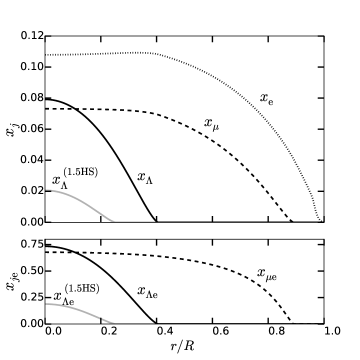
Figure 1: Upper panel: number fraction of electrons $x_{\rm e}$ (dotted line), muons $x_{\mu}$ (dashed line), and $\Lambda$ hyperons $x_{\Lambda}$ (solid black line) as a function of fractional radius $r/R$ for the $1.6M_{\odot}$ HS model. For comparison, we also show $x_{\Lambda}$ for the $1.5M_{\odot}$ HS model (solid grey line). Bottom panel: number of muons per electron $x_{\mu\rm e}$ (dashed line) and $\Lambda$ hyperons per electron $x_{\Lambda\rm e}$ (solid black line) for the $1.6M_{\odot}$ HS model, and $x_{\Lambda\rm e}$ for the $1.5M_{\odot}$ HS model (solid grey line).

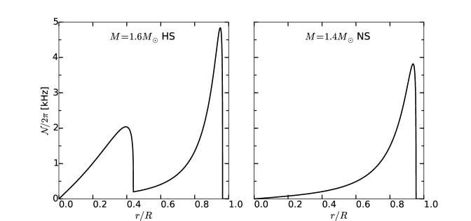
Figure 2: Brunt-Väisälä frequency $\mathcal{N}/2\pi$ for the $1.6M_{\odot}$ HS (left panel) and the $1.4M_{\odot}$ NS (right panel). Both models have a muonic contribution that peaks in the outer core. The HS has an additional contribution due to hyperons that peaks in the inner core. Note that we evaluate the frequencies in the Newtonian limit (eq. 4).

The conditions for chemical equilibrium due to weak interactions are (Dommes & Gusakov, 2016),

$$\mu_{\rm n}=\mu_{\rm p}+\mu_{\rm e},$$ (1)

$$\mu_{\rm n}=\mu_{\Lambda},$$ (2)

$$\mu_{\rm e}=\mu_{\mu},$$ (3)

where $\mu_{j}$ is the chemical potential of particle species $j$, with $j$ being either a neutron (n), proton (p), $\Lambda$ hyperon ($\Lambda$), electron (e), or muon ($\mu$). These conditions, along with the equations of stellar structure, determine the composition profile for each star. Because of the presence of hyperons, the equation of state has four degrees of freedom instead of the three in YW17. In particular, we parametrize the thermodynamic relations in terms of the pressure $P$, the neutron chemical potential $\mu_{\rm n}$, the muon-to-electron ratio $x_{\mu\rm e}=x_{\mu}/x_{\rm e}$, and the $\Lambda$-to-electron ratio $x_{\Lambda\rm e}=x_{\Lambda}/x_{\rm e}$, where $x_{j}=n_{j}/n_{\rm b}$ is the number fraction of species $j$ per baryon and $n_{j}$ is its number density.

In Table 1, we give the values of the following parameters for our three models: total mass $M$, radius $R$, central density $\rho_{0}$, radius below which $\Lambda$ hyperons are present $R_{\Lambda}$, radius below which muons are present $R_{\mu}$, and radius of the core-crust interface $R_{\textrm{cc}}$ (defined as where the baryon density $n_{\rm b}=0.08\textrm{ fm}^{-3}$). In Fig. 1, we show the composition profile for the $1.6M_{\odot}$ HS model and for comparison, $x_{\Lambda}(r)$ and $x_{\Lambda\rm e}(r)$ for the $1.5M_{\odot}$ HS model.

Based on the discussion in YW17 (see their Section 2.1 and Appendix A), in the Newtonian limit the Brunt-Väisälä (i.e., buoyancy) frequency is given by

$$\mathcal{N}^{2}= -\frac{1-\epsilon_{\textrm{n}}}{1-x_{\textrm{n}}-\epsilon_{\textrm{n}}}\frac{g}{\rho}\sum_{j=\mu,\Lambda}\left(\frac{\partial\rho}{\partial x_{j\rm e}}\right)\frac{\text{d}x_{j\rm e}}{\text{d}r},$$ (4)

where the partial derivative is evaluated by holding the three other thermodynamic parameters fixed ($P$, $\mu_{\rm n}$, and $x_{i\rm e}$ for $i\neq j$), $g(r)$ is the gravitational acceleration at radius $r$, and $\epsilon_{\rm n}$ is the superfluid entrainment function (YW17, see also Prix & Rieutord 2002). Numerical values for entrainment are provided in Gusakov et al. (2014) but using a different parameterization.

In the core, we evaluate the buoyancy using equation (4). In the crust, we follow YW17 and assume for simplicity that the crust is neutrally buoyant ($\mathcal{N}=0$); this does not significantly affect the core g-modes of interest here since the crust contains only a small fraction of the mass. In Fig. 2 we show $\mathcal{N}$ for the $1.4M_{\odot}$ NS model (right panel) and the $1.6M_{\odot}$ HS model (left panel). Whereas the $1.4M_{\odot}$ model contains only a single $\mathcal{N}$ peak (due to the muon gradient $\text{d}x_{\mu\rm e}/\text{d}r$), the $1.6M_{\odot}$ HS model contains two $\mathcal{N}$ peaks (one due to the muon gradient $\text{d}x_{\mu\rm e}/\text{d}r$ and one at higher densities due to the $\Lambda$ hyperon gradient $\text{d}x_{\Lambda\rm e}/\text{d}r$). As we show in the next section, this additional peak leads to a new type of g-mode, i.e., hyperonic g-modes.

We assume that $x_{\mu\rm e}$ and $x_{\Lambda\rm e}$ do not vary during oscillations of the normal fluid; i.e., the composition is “frozen" and thus the perturbed fluid element is out of chemical equilibrium. Reisenegger & Goldreich (1992) consider the timescale for the proton fraction $x_{\rm p}$ in a normal fluid NS to relax towards chemical equilibrium due to Urca processes ($x_{p}$ is the source of buoyancy in a normal fluid NS). They show that for even a moderately warm NS, the relaxation timescale is much longer than the oscillation period of low-order g-modes and therefore, to a very good approximation, $x_{\rm p}$ is frozen within the fluid element. Similarly, to check whether $x_{\Lambda\rm e}$ is frozen, we must consider the direct Urca process $\Lambda\to{\rm p}+{\rm L}+\bar{\nu}_{\rm L}$, where the lepton in the reaction $\textrm{L}=\rm{e}$ or $\mu$. In Appendix A we show that the corresponding relaxation timescale is much longer than the oscillation period of low order hyperonic g-modes and therefore the assumption of frozen composition should also hold for these modes.

3 EIGENMODES OF A SUPERFLUID HYPERON STAR

The oscillation equations of a superfluid HS are similar to those of a superfluid NS and can be written as (Prix & Rieutord 2002, YW17)

$$\boldsymbol{\nabla}\cdot(\rho_{\textrm{c}}\boldsymbol{\xi}_{\textrm{c}})+\delta\rho_{\textrm{c}}=0,$$ (5)

$$\boldsymbol{\nabla}\cdot(\rho_{\textrm{n}}\boldsymbol{\xi}_{\textrm{n}})+\delta\rho_{\textrm{n}}=0,$$ (6)

$$\sigma^{2}\left[\boldsymbol{\xi}_{\textrm{c}}-\epsilon_{\textrm{c}}(\boldsymbol{\xi}_{\textrm{c}}-\boldsymbol{\xi}_{\textrm{n}})\right]=\boldsymbol{\nabla}\left(\delta\tilde{\mu}_{\textrm{c}}+\delta\Phi\right),$$ (7)

$$\sigma^{2}\left[\boldsymbol{\xi}_{\textrm{n}}+\epsilon_{\textrm{n}}(\boldsymbol{\xi}_{\textrm{c}}-\boldsymbol{\xi}_{\textrm{n}})\right]=\boldsymbol{\nabla}\left(\delta\tilde{\mu}_{\textrm{n}}+\delta\Phi\right),$$ (8)

$$\nabla^{2}\delta\Phi=4\pi G(\delta\rho_{\textrm{c}}+\delta\rho_{\textrm{n}}),$$ (9)

where we assume that the perturbed quantities have a time dependence $e^{\rm{i}\sigma t}$, $\delta\mathcal{Q}(\boldsymbol{x})$ denotes the Eulerian perturbation of a quantity $\mathcal{Q}$ at position $\boldsymbol{x}$, subscript ‘n’ denotes the neutron superfluid flow, and subscript ‘c’ denotes the normal fluid flow (consisting of the charged particles and the $\Lambda$ hyperons; we continue to use a subscript c in order to match the notation used in Prix & Rieutord (2002) and YW17). The other quantities are the mass densities $\rho_{\textrm{c(n)}}$ (the total density $\rho=\rho_{\rm c}+\rho_{\rm n}$), the perturbed specific chemical potentials $\delta\tilde{\mu}_{\textrm{c(n)}}$, the Lagrangian displacements $\boldsymbol{\xi}_{\textrm{c(n)}}$, the perturbed gravitational potential $\delta\Phi$, and the entrainment function $\epsilon_{\rm c}=\epsilon_{\rm n}\rho_{\rm n}/\rho_{\rm c}$ (see YW17 for further details).

Although the oscillation equations take a simple form when written in terms of $\boldsymbol{\xi}_{\textrm{c}}$ and $\boldsymbol{\xi}_{\textrm{n}}$, it is more convenient to express the tidal excitation of modes in terms of the mass-averaged flow $\boldsymbol{\xi}_{+}$ and the difference flow $\boldsymbol{\xi}_{-}$, where

$$\boldsymbol{\xi}_{+}=\frac{1}{\rho}\left(\rho_{\textrm{c}}\boldsymbol{\xi}_{\textrm{c}}+\rho_{\textrm{n}}\boldsymbol{\xi}_{\textrm{n}}\right),$$ (10)

$$\boldsymbol{\xi}_{-}=\left(1-\epsilon_{\textrm{n}}-\epsilon_{\textrm{c}}\right)\left(\boldsymbol{\xi}_{\textrm{c}}-\boldsymbol{\xi}_{\textrm{n}}\right).$$ (11)

When solving the oscillation equations, we choose ($\boldsymbol{\xi}_{+}$, $\boldsymbol{\xi}_{\rm n}$, $\delta P$, $\delta\tilde{\mu}_{\textrm{n}}$, $\delta\Phi$) to be our independent variables. We can then use equations (10) and (11) to calculate $\boldsymbol{\xi}_{\rm c}$ and $\boldsymbol{\xi}_{-}$. Since the Lagrangian perturbations to $x_{\mu\rm e}$ and $x_{\Lambda\rm e}$ vanish for a frozen composition, we can use the chain rule to express the density perturbation as

$$\delta\rho_{\textrm{c}} =\left(\frac{\partial\rho_{\textrm{c}}}{\partial P}\right)\delta P+\left(\frac{\partial\rho_{\textrm{c}}}{\partial\tilde{\mu}_{\textrm{n}}}\right)\delta\tilde{\mu}_{\textrm{n}}-\sum_{j=\mu,\Lambda}\left(\frac{\partial\rho_{\textrm{c}}}{\partial x_{j\rm e}}\right)\frac{\text{d}x_{j\rm e}}{\text{d}r}\xi^{r}_{\rm c},$$ (12)

and similarly for $\delta\rho_{\textrm{n}}$, where $\xi^{r}_{\rm c}(r)$ denotes the radial dependence of the radial component of $\boldsymbol{\xi}_{\rm c}$ (the angular dependence is given by the spherical harmonic function $Y_{lm}(\theta,\phi)$ of degree $l$ and order $m$). As we show in YW17 (see also Lindblom & Mendell 1994; Andersson et al. 2004), the operator $\mathcal{L}$ corresponding to equations (5)-(9) is Hermitian with respect to the inner product

$$\left\langle\begin{bmatrix}\boldsymbol{\xi}_{+}\\ \boldsymbol{\xi}_{-}\end{bmatrix},\begin{bmatrix}\boldsymbol{\xi}_{+}^{\prime}\\ \boldsymbol{\xi}_{-}^{\prime}\end{bmatrix}\right\rangle=\int\text{d}^{3}x\begin{bmatrix}\boldsymbol{\xi}_{+}^{\ast}&\boldsymbol{\xi}_{-}^{\ast}\end{bmatrix}\begin{bmatrix}\rho&0\\ 0&\tilde{\rho}\end{bmatrix}\begin{bmatrix}\boldsymbol{\xi}_{+}^{\prime}\\ \boldsymbol{\xi}_{-}^{\prime}\end{bmatrix},$$ (13)

where

$$\tilde{\rho}=\frac{\rho_{\textrm{c}}\rho_{\textrm{n}}}{(1-\epsilon_{\textrm{n}}-\epsilon_{\textrm{c}})\rho}.$$ (14)

The set of eigenmodes thus forms an orthonormal base. We use the same boundary conditions as YW17 and normalize the modes such that

$$\sigma_{a}^{2}\left\langle\begin{bmatrix}\boldsymbol{\xi}_{a+}\\ \boldsymbol{\xi}_{a-}\end{bmatrix},\begin{bmatrix}\boldsymbol{\xi}_{b+}\\ \boldsymbol{\xi}_{b-}\end{bmatrix}\right\rangle=E_{0}\delta_{ab},$$ (15)

where $\sigma_{a}$ is the eigenvalue of mode $a$ and $E_{0}=GM^{2}/R$.

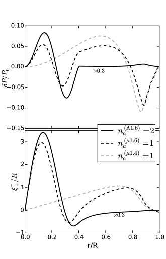
Figure 3: Structure of the second hyperonic g-mode $n_{a}^{(\Lambda 1.6)}=2$ (solid black lines) and the first muonic g-mode $n_{a}^{(\mu 1.6)}=1$ (dashed black lines) of the $1.6M_{\odot}$ HS and the first g-mode $n_{a}^{(\mu 1.4)}=1$ of the 1.4 $M_{\odot}$ NS (dashed grey lines). All three modes have spherical degree $l_{a}=2$. The upper panel shows the Eulerian perturbation of the pressure $\delta P$ in units of the central pressure $P_{0}$. The lower panel shows the radial component of the mass-averaged Lagrangian displacement $\xi^{r}_{+}$ in units of $R$. All quantities are normalized according to Equation (15); for display purposes, those corresponding to the $n_{a}^{(\Lambda 1.6)}=2$ mode are multiplied by an additional factor of 0.3.

As Dommes & Gusakov (2016) first showed, the core g-modes of an HS can be classified into two types: ‘hyperonic’ g-modes and ‘muonic’ g-modes. The hyperonic g-modes are primarily supported by the $\Lambda$ hyperon gradient and are concentrated in the inner core, while the muonic g-modes are supported by a combination of the $\Lambda$ hyperon and muon gradients and span both the inner and outer core. In Fig. 3 we show the structure of the second hyperonic g-mode $n_{a}^{(\Lambda 1.6)}=2$ and the first muonic g-mode $n_{a}^{(\mu 1.6)}=1$ of our $1.6M_{\odot}$ HS model. In the superscript, $\Lambda 1.6$ ($\mu 1.6$) stands for the hyperonic (muonic) modes of the 1.6 $M_{\odot}$ HS model. We will use this labeling convention throughout the paper. For comparison, we also show the first g-mode of our $1.4M_{\odot}$ NS model. All three g-modes have angular degree $l_{a}=2$ and thus couple to the $l=2$ harmonic of the tide.

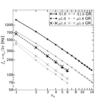
Figure 4: Eigenfrequencies $f_{a}=\sigma_{a}/2\pi$ of $l_{a}=2$ g-modes calculated with the Newtonian oscillation equations (black lines) and the GR oscillation equations (grey lines). For the $1.6M_{\odot}$ HS model, we show the hyperonic modes with filled circles connected by solid lines and the muonic modes with filled circles connected by dashed lines. For the $1.4M_{\odot}$ NS model, which only have muonic g-modes, we use crosses connected by dashed lines.

In Fig. 4 we show the eigenfrequencies $f_{a}=\sigma_{a}/2\pi$ of the first several $l_{a}=2$ g-modes of our $1.6M_{\odot}$ HS and $1.4M_{\odot}$ NS models. To guide the eye, we use straight lines to connect each of the hyperonic modes (solid) and, separately, each of the muonic modes (dashed). As we describe in Section 2, in order to build HSs without complicating the dynamical tide calculation, we solve the TOV equations to construct the background models but the Newtonian equations to calculate the g-modes and tidal driving. We partially assess the impact of this hybrid approach by redoing the calculation of the g-modes using the GR oscillation equations. For this calculation, we ignore the gravitational perturbations (i.e., we adopt the Cowling approximation) and solve the superfluid GR oscillation equations (see, e.g., Dommes & Gusakov 2016; Passamonti et al. 2016). We find that our hybrid approach overestimates the g-mode eigenfrequencies by $\simeq 70\%$ (see grey lines in Fig. 4). For example, the highest frequency $l_{a}=2$ hyperonic g-mode in the $1.6M_{\odot}$ HS has a frequency of $f_{a}^{\rm(GR)}=743\textrm{ Hz}$ in the fully relativistic calculation (as seen by an observer at infinity) compared to $f_{a}=1271\textrm{ Hz}$ in the hybrid calculation. Nevertheless, as we show in Section 4, the dynamical tide phase shift is independent of the eigenfrequency $f_{a}$ (in our normalization) and is therefore unaffected by the overestimate of $f_{a}$. There is still an error due to our hybrid calculation of the tidal coupling strength, but we argue in Section 4 that this should not be too significant.

Consistent with the asymptotic properties of high-order g-modes (Aerts et al., 2010), we find that for modes with $n_{a}^{(j)}\gtrsim\textrm{ few}$, the GR oscillation equations yield $l_{a}=2$ eigenfrequencies that are well approximated by $f_{a}^{(j,\textrm{GR})}={f_{0}^{(j)}}/{n_{a}^{(j)}}$, where $f_{0}^{(j)}=\{1020,410,460,500,510\}\textrm{ Hz}$ for $j=\{\Lambda 1.6,\mu 1.6,\Lambda 1.5,\mu 1.5,\mu 1.4\}$, respectively. We find that the characteristic frequency $f_{0}^{(\Lambda)}$ of the hyperonic modes scales almost linearly with the size of the hyperonic core $R_{\Lambda}$. This is because $f_{0}^{(\Lambda)}\propto\int_{0}^{R_{\Lambda}}\mathcal{N}d\ln r$ and for $r\lesssim R_{\Lambda}$, the density $\rho\simeq\textrm{ constant}$ and $\mathcal{N}\propto r$.

4 TIDAL DRIVING AND PHASE SHIFT of the gravitational waveform

Following YW17 (see also Lai 1994; Weinberg et al. 2012), we solve for the resonant tidal excitation of g-modes by expanding the tidal displacement field as

$$\begin{bmatrix}\boldsymbol{\xi}_{+}(\boldsymbol{x},t)\\ \boldsymbol{\xi}_{-}(\boldsymbol{x},t)\end{bmatrix}=\sum_{a}b_{a}(t)\begin{bmatrix}\boldsymbol{\xi}_{a+}(\boldsymbol{x})\\ \boldsymbol{\xi}_{a-}(\boldsymbol{x})\end{bmatrix},$$ (16)

where the subscript $a=\{n_{a},\ l_{a},\ m_{a}\}$ denotes a specific eigenmode of the NS and $b_{a}(t)$ is the time-dependent, dimensionless amplitude of mode $a$ (a mode with amplitude $|b_{a}|=1$ has energy $E_{0}=GM^{2}/R$). Inserting this expansion into the linear superfluid oscillation equations (5)-(9) and including the time-dependent tidal potential ($\delta\Phi\rightarrow\delta\Phi+U$) yields the mode amplitude equation

$$\ddot{b}_{a}+\sigma_{a}^{2}b_{a}=\sigma_{a}^{2}U_{a}(t),$$ (17)

where the tidal driving coefficient

$$U_{a}(t)=\frac{M^{\prime}}{M}\sum_{l\geq 2,m}W_{lm}Q_{alm}\left(\frac{R}{D(t)}\right)^{l+1}e^{-im\psi(t)}.$$ (18)

Here $M^{\prime}$ is the mass of the companion, $lm$ are harmonics of the tidal potential, the coefficients $W_{lm}=4\pi(2l+1)^{-1}Y_{lm}(\pi/2,0)$ are of order unity for the dominant harmonics (Press & Teukolsky, 1977), $D(t)$ is the orbital separation, and $\psi(t)$ is the orbital phase.

The time-independent, dimensionless tidal coupling coefficient (sometimes referred to as the tidal overlap integral)

$$Q_{alm}=\frac{1}{MR^{l}}\int\text{d}^{3}x\rho\,\boldsymbol{\xi}_{a+}^{\ast}\cdot\boldsymbol{\nabla}\left(r^{l}Y_{lm}\right).$$ (19)

By angular momentum conservation, $Q_{alm}$ is non-zero only if $l_{a}=l$ and $m_{a}=m$. Based on our numerical calculations, we find that the $Q_{alm}$ of our different models and mode types are approximately given by

$$|Q_{alm}^{(j)}|=Q_{0}n_{a}^{-\alpha},$$ (20)

where

$$\alpha\approx 2.5\hskip 7.11317pt\textrm{and}$$

$$Q^{(j)}_{0}=\{1.7,\,3.6,\,1.6,\,3.5,\,4.0\}\times 10^{-3},$$ (21)

for $j=\{\Lambda 1.6,\mu 1.6,\Lambda 1.5,\mu 1.5,\mu 1.4\}$, respectively.

Although these values are based on the hybrid calculation (GR background and Newtonian oscillations), we expect the error due to this inconsistency to be relatively small. As an approximate measure of the correction, we computed $|Q_{alm}|$ for the $1.4M_{\odot}$ NS model but with the background constructed using the Newtonian structure equations rather than the TOV equations (we could not perform such a test for the HS model because a $2.0M_{\odot}$ Newtonian model does not contain hyperons). We find that $Q_{alm}$ changes by at most $5\%$, which suggests that our hybrid model gives a reasonably accurate estimate of the tidal coupling strength. Indeed, given that $GM/Rc^{2}\approx 20\%$, we do not expect relativistic corrections to be much bigger than a few tens of percent.

We numerically solve the amplitude equation (17) of the resonantly driven g-modes and find that the result is in good agreement with the analytic solution given by the stationary-phase approximation (Lai, 1994; Reisenegger & Goldreich, 1994). The GW phase shift induced by the resonant excitation of each mode is therefore approximately given by (YW17)

$$\delta\phi_{a}=-\frac{5\pi^{2}}{2048}k^{\prime}\left(\frac{GM}{Rc^{2}}\right)^{-5}\sum_{m=\pm 2}|Q_{a2m}|^{2},$$ (22)

where $k^{\prime}=2/[q(1+q)]$, $q=M^{\prime}/M$, and here the subscript $a$ already accounts for the contributions from both the $m_{a}=2$ and $m_{a}=-2$ modes. Since $\delta\phi_{a}$ depends on $f_{a}$ only through $|Q_{alm}|$, and we expect that our hybrid approach accurately estimates $|Q_{alm}|$ to within a few tens of percent, our estimate of $\delta\phi_{a}\propto|Q_{alm}|^{2}$ should be accurate to within a factor of order unity.

In Table 2 we list $f^{\rm(GR)}_{a}$ (see grey lines in Figure 4) and $\delta\phi_{a}$ for the three-lowest order $l_{a}=2$ g-modes of each type, for each stellar model. Numerically, we find that summing over all of the resonantly excited modes yields a total cumulative phase shift

$$\delta\phi^{\textrm{(1.6HS)}}=-4.3\times 10^{-3}k^{\prime},$$ (23)

$$\delta\phi^{\textrm{(1.5HS)}}=-6.7\times 10^{-3}k^{\prime},$$ (24)

$$\delta\phi^{\textrm{(1.4NS)}}=-9.9\times 10^{-3}k^{\prime},$$ (25)

where $\delta\phi^{\textrm{(HS)}}$ accounts for both the hyperonic modes and muonic modes.

As can be gleaned from Table 2 [also eqs. (20) - (22)], the total phase shift is dominated by the contributions of the $n_{a}=1$ g-modes (the modes with the highest frequency). The phase shifts due to muonic modes are insensitive to whether hyperons are present in the core and decrease with increasing HS/NS mass. In the HS models, the cumulative phase shift due to the muonic g-modes is about five times larger than that due to the hyperonic g-modes. Moreover, comparing the $1.6M_{\odot}$ HS model to the $1.5M_{\odot}$ HS model, we find that the phase shift due to the hyperonic modes is relatively insensitive to the size of the hyperon core $R_{\Lambda}$, in contrast to the eigenfrequency spectrum which is shifted to lower frequencies as the mass of the hyperon core decreases (see discussion at end of Section 3).

Table 2: Eigenfrequencies $f_{a}^{\rm(GR)}$ and gravitational waveform phase shift $\delta\phi_{a}$ for the three-lowest order $l_{a}=2$ g-modes for each stellar model. The format is $\left\{f_{a}/100\textrm{ Hz},\,|\delta\phi_{a}|/\textrm{rad}\right\}$.

$j$	$n_{a}^{(j)}=1$	$n_{a}^{(j)}=2$	$n_{a}^{(j)}=3$
$\Lambda 1.6$	{7.4,   5.5e-4}	{4.3,   3.4e-4}	{3.0,   3.6e-7}
$\mu 1.6$	{4.1,   3.4e-3}	{2.0,   1.6e-5}	{1.3,   1.2e-5}
$\Lambda 1.5$	{4.1,   1.1e-3}	{2.5,   1.6e-7}	{1.4,   6.6e-7}
$\mu 1.5$	{4.5,   5.4e-3}	{2.4,   6.6e-6}	{1.6,   2.1e-5}
$\mu 1.4$	{4.6,   9.8e-3}	{2.4,   3.6e-7}	{1.6,   3.0e-5}

5 DETECTABILITY OF THE MODE RESONANCES

In this section we estimate the detectability of the dynamical tide phase shift using the Fisher matrix formalism (Cutler & Flanagan, 1994). In Section 5.1, we describe how we model the GW signal and the detectability of the resonances based on single events and multiple stacked events. In Section 5.2, we present our detectability estimates for Advanced LIGO and proposed third generation GW detectors.

5.1 Modeling the detectability

Following Cutler & Flanagan (1994), if we assume a strong GW strain signal $h(t)$ and Gaussian detector noise, then the signal parameters $\theta^{i}$ have a probability distribution $p(\theta^{i})\propto\exp\left[-(1/2)\Gamma_{ij}\text{d}\theta^{i}\text{d}\theta^{j}\right]$, where $\text{d}\theta^{i}=\theta^{i}-\hat{\theta}^{i}$ is the difference between the parameters and their best fit values $\hat{\theta}^{i}$ and

$$\Gamma_{ij}=\left(\frac{\partial h}{\partial\theta^{i}}\Bigg{|}\frac{\partial h}{\partial\theta^{j}}\right)$$ (26)

is the Fisher information matrix. The parentheses denote the inner product

$$\left(h_{1}|h_{2}\right)=2\int_{0}^{\infty}\frac{\tilde{h}^{\ast}_{1}(f)\tilde{h}_{2}(f)+\tilde{h}_{1}(f)\tilde{h}_{2}^{\ast}(f)}{S_{n}(f)}\text{d}f,$$ (27)

where $\tilde{h}_{1}$ and $\tilde{h}_{2}$ are the Fourier transforms of $h_{1}$ and $h_{2}$ and $S_{n}(f)$ is the strain noise power spectral density. The signal-to-noise ratio (SNR) of a signal $h$ is given by $\textrm{SNR}=(h|h)^{1/2}$ and the root-mean-square (rms) measurement error in $\theta^{i}$ is given by a diagonal element of the inverse Fisher matrix

$$\Delta\theta^{i}=\sqrt{\left(\boldsymbol{\Gamma}^{-1}\right)^{ii}}.$$ (28)

If the rms error in, say, the phase shift due to a particular resonance $\Delta(\delta\phi_{a})$ is smaller than $\delta\phi_{a}$, then that phase shift is detectable.

The above analysis is based on the detection of a single inspiral event. We can roughly estimate how stacking multiple events would affect the measurement accuracy by using the approach given in Markakis et al. (2010); a more precise estimate would require a fully Bayesian investigation and is beyond the scope of this paper (see, e.g., the recent studies of the detectability of the equilibrium tide phase shift by Del Pozzo et al. 2013; Lackey & Wade 2015; Agathos et al. 2015). The estimate assumes that the events are homogeneously distributed in a sphere of effective radius $d^{\rm eff}_{\rm max}$ and that the error in each parameter $\Delta\theta$ scales linearly with effective distance $d^{\rm eff}<d^{\rm eff}_{\rm max}$. Then, Markakis et al. (2010) show that the rms error averaged over all of the events is

$$\langle{\Delta\theta}\rangle\approx\frac{\Delta\theta_{\rm ref}}{d^{\rm eff}_{\rm ref}\sqrt{4\pi\mathcal{R}P_{\rm obs}d^{\rm eff}_{\rm max}}},$$ (29)

where $\Delta\theta_{\rm ref}$ is the rms error of parameter $\theta$ from a single reference event at effective distance $d_{\rm ref}^{\rm eff}$, $\mathcal{R}$ is the event rate per unit time per unit volume, and $P_{\rm obs}$ is the total observation period. In the above calculation we ignore the cosmological expansion and assume that the event rate is constant.

Similar to Balachandran & Flanagan (2007), who also studied the detectability of mode resonances (see also Flanagan & Racine 2007), we assume that the frequency-domain GW signal has the form

$$\tilde{h}(f)=\mathcal{A}f^{-7/6}e^{i\Psi(f)},$$ (30)

where the amplitude (Maggiore, 2007)

$$\mathcal{A}=\left(\frac{5}{24\pi^{4/3}}\right)^{1/2}\left(\frac{G\mathcal{M}}{c^{3}}\right)^{-5/6}\frac{\mathcal{K}}{d}.$$ (31)

Here $\mathcal{M}=[(MM^{\prime})^{3}/(M+M^{\prime})]^{1/5}$ is the chirp mass, $d$ is the distance to the source, and $\mathcal{K}$ is the antenna response (for an optimally oriented source $\mathcal{K}=1$). Our model of the phase evolution $\Psi(f)$ accounts for the zeroth order post-Newtonian point-particle contribution and for the resonant tidal excitation of individual g-modes. We ignore higher order post-Newtonian terms, spin, the equilibrium tide, and nonlinear tidal effects (such as those considered in Essick et al. 2016), and assume that the signal shuts off at the gravitational wave frequency corresponding to the inner-most stable circular orbit $f=2f_{\rm ISCO}\simeq 1.6\times 10^{3}\textrm{Hz }[2.8M_{\odot}/(M+M^{\prime})]$ (Cutler & Flanagan, 1994; Poisson & Will, 1995). In Appendix B we show that under these assumptions,

$$\Psi(f)=\Psi_{\rm pp}(f)-\sum_{a}\left(1-\frac{f}{f_{a}}\right)\delta\phi_{a}\Theta\left(f-f_{a}\right),$$ (32)

where, by the stationary-phase approximation, the point-particle phase is (Cutler & Flanagan, 1994)

$$\Psi_{\rm pp}(f)=2\pi ft_{c}-\phi_{c}-\frac{\pi}{4}+\frac{3}{4}\left(\frac{8\pi G\mathcal{M}f}{c^{3}}\right)^{-5/3},$$ (33)

$\delta\phi_{a}$ is the phase shift due to the tidal resonance with a mode $a$ with eigenfrequency $f_{a}$, and $\Theta\left(f-f_{a}\right)$ is the Heaviside step function. Here $t_{c}$ and $\phi_{c}$ are constants of integration that set a reference time and phase. The duration of each resonance is, in general, much shorter than the orbital decay timescale due to radiation reaction (their ratio is $\simeq 0.1\times[(\mathcal{M}/1.2M_{\odot})(f/500\text{ Hz})]^{5/6}$; see Lai 1994; Flanagan & Racine 2007; Balachandran & Flanagan 2007). We therefore model the resonance as an instantaneous process, which should be a good approximation since nearly all the g-modes we consider have $f_{a}^{\rm(GR)}<500\textrm{ Hz}$ (the one exception is the $n_{a}=1$ hyperonic g-mode of the $1.6M_{\odot}$ HS model which has $f_{a}^{\rm(GR)}=740\textrm{ Hz}$).

Since the phase shift is dominated by the resonant excitation of the lowest order mode, for simplicity we do not sum over the modes in our waveform model but instead just consider the phase shift due to a single mode. Our model therefore depends on 6 parameters: $\mathcal{A}$, $\mathcal{M}$, $t_{c}$, $\phi_{c}$, $f_{a}$, and $\delta\phi_{a}$. Flanagan & Racine (2007) also consider the effect of phase shifts on the GW signal, although their model is written in terms of the phase of the time-domain waveform $\phi(t)$ (their equation 1.9) rather than the frequency-domain waveform $\Psi(f)$. In Appendix B we show that the two treatments are consistent.

Before examining the numerical results, note that

$$\frac{\partial\tilde{h}}{\partial(\delta\phi_{a})}=-\textrm{i}\left(1-\frac{f}{f_{a}}\right)\Theta\left(f-f_{a}\right)\tilde{h},$$ (34)

$$\frac{\partial\tilde{h}}{\partial f_{a}}=-\textrm{i}\delta\phi_{a}\frac{f}{f_{a}^{2}}\Theta\left(f-f_{a}\right)\tilde{h}.$$ (35)

Note that the $(1-f/f_{a})$ factor eliminates the $\delta$-function at $f=f_{a}$ stemming from the derivative of $\Theta$. By equation (28), we see that $\Delta(\delta\phi_{a})$ and $\Delta f_{a}$ both vary linearly with distance (and thus inversely with SNR) and that $\Delta(\delta\phi_{a})$ is independent of $\delta\phi_{a}$ whereas $\Delta f_{a}\propto(\delta\phi_{a})^{-1}$. Conceptually, these last two properties reflect the fact that the measurability of phase shifts $\Delta(\delta\phi_{a})$ is mostly determined by how much SNR accumulates before and after the resonance (which is independent of $\delta\phi_{a}$ itself), whereas the larger $\delta\phi_{a}$ is, the easier it is to localize the frequency of the resonance (and thus the smaller $\Delta f_{a}$ is). Lastly, because the dominating g-modes are excited at frequencies higher than the most sensitive band of ground-based GW detectors ($\approx 70\textrm{ Hz}$), larger $f_{a}$ have larger $\Delta(\delta\phi_{a})$ and $\Delta(f_{a})$ and thus worse detectability. This is different from the results in Balachandran & Flanagan (2007) who found that increasing $f_{a}$ would make the detection easier, as Balachandran & Flanagan (2007) considered modes that were excited at frequencies lower than the most sensitive band.

5.2 Detectability with second and third generation detectors

Table 3: Threshold distance $d_{\rm th}^{\rm hor}$ out to which dynamical tide resonances are detectable [$\Delta(\delta\phi_{a})=|\delta\phi_{a}|$] assuming a single merger event.

$f_{a}$ [Hz]	$|\delta\phi_{a}|$ [rad]	Detector	$d_{\rm th}^{\rm hor}$ [Mpc]	SNR	$\Delta f_{a}$ [Hz]
		aLIGO	1.9	1.9e+3	2.4e+2
450	0.01	CE	27	5.5e+3	2.1e+2
		ET-D	17	2.5e+3	2.2e+2
		aLIGO	0.19	1.9e+4	2.4e+2
450	0.001	CE	2.7	5.5e+4	2.1e+2
		ET-D	1.7	2.5e+4	2.2e+2
		aLIGO	0.06	5.7e+4	2.5e+2
750	0.001	CE	0.8	1.8e+5	2.3e+2
		ET-D	0.5	8.1e+4	2.4e+2

For the numerical results, we take $M=M^{\prime}=1.4M_{\odot}$ (using $M=M^{\prime}=1.5M_{\odot}$ or $1.6M_{\odot}$ in the Fisher matrix calculation changes the rms errors only by $\lesssim 10\%$). Since the values of $t_{c}$ and $\phi_{c}$ do not affect the evaluation of $\Delta(\delta\phi)$ and $\Delta f_{a}$, we set them equal to zero. We show results for three sets of tidal parameters, one with $f_{a}=450$ Hz and $\delta\phi_{a}=0.01\textrm{ rad}$, corresponding to the lowest order muonic g-mode in the NS/HS model, one with $f_{a}=450\text{ Hz}$ and $\delta\phi_{a}=0.001\text{ rad}$ for the first hyperonic mode in the $1.5M_{\odot}$ HS model, and one with $f_{a}=750\text{ Hz}$ and $\delta\phi_{a}=0.001\text{ rad}$ for the first hyperonic mode in $1.6M_{\odot}$ HS. Higher order g-modes resonate at lower frequencies and have smaller $\Delta(\delta\phi_{a})$ because more SNR is accumulated after their resonances [eq. (34)]. However, because of the steep falloff of $\delta\phi_{a}$ with decreasing frequency [increasing $n_{a}$; see eq. (20)], it is much more difficult to detect their phase shifts.

For the detector noise, we consider the noise curves of Advanced LIGO (aLIGO) at design sensitivity (LIGO Scientific Collaboration et al., 2015), and the noise curves of proposed third generation detectors including the Cosmic Explorer (CE; Abbott et al. 2017) and the Einstein Telescope (specifically, ET-D; Hild et al. 2011). For simplicity we consider here only the detectability of a single detector instead of a network of detectors (Schutz, 2011). We also ignore the tidal phase shift due to the companion NS/HS which should increase $\delta\phi_{a}$ by a factor of two if $M=M^{\prime}$.

Our analysis neglects systematic uncertainties due to calibration errors in the instruments. The current calibration uncertainty of aLIGO is somewhat larger than the phase shift due to dynamic tides (the phase uncertainty is $\simeq 0.03\textrm{ rad}$ at 450 Hz; Vitale et al. 2012; The LIGO Scientific Collaboration et al. 2016). Regardless, we show that for aLIGO the measurement errors dominate ($\Delta(\delta\phi_{a})\ga 0.1\textrm{ rad}$ even with event stacking) and preclude detecting the dynamical tide with aLIGO. As for the third generation detectors, currently there is no published estimate of their expected calibration performance. We therefore ignore this effect in our study and work under the assumption that it will be at least a factor of $\sim 10$ better than aLIGO’s.

5.2.1 Single events

In Table 3 we show the threshold horizon distance $d_{\rm th}^{\rm hor}$ out to which different GW detectors can measure tidal resonances assuming a single merger event. Here $d_{\rm th}^{\rm hor}$ is defined to be the distance at which an event has $\Delta(\delta\phi_{a})=\delta\phi_{a}$ assuming an optimal antenna response $\mathcal{K}=1$. We also give the events corresponding SNR and $\Delta f_{a}$. For the dominating muonic mode, aLIGO can detect such a feature only for an event happening within 1.9 Mpc (i.e., within the Local Group). With the third generation detectors, this horizon distance can be pushed out to $\approx 20-30\textrm{ Mpc}$, and thus could include the Virgo Cluster ($16\text{ Mpc}$). If we account for the random source orientation (by dividing $d_{\rm th}^{\rm hor}$ by 2.3) and assume the ‘most-likely’ event rate of $\mathcal{R}=10^{3}\textrm{ Gpc${}^{-3}$ yr${}^{-1}$}$ (Abadie & et al. 2010; Abbott et al. 2016), we find that such an event should happen only once every $\approx 150\textrm{ yr}$ at CE sensitivity (here we ignore that the Universe is far from being homogeneous in such a local range and simply assume that the sources are uniformly distributed).

In terms of SNR, the detection of g-modes from a single event typically requires an $\text{SNR}\gtrsim 2000$, with the exact number depending on the detailed shape of the sensitivity curve. As a comparison, for a typical event with $\text{SNR}=12$, with aLIGO we can only measure $\Delta(\delta\phi_{a})=1.9\textrm{ rad}$, which is more than two orders of magnitude larger than $\delta\phi_{a}$, and $\Delta f_{a}=4.7\times 10^{4}\textrm{ Hz}$, which is greater than the entire detector bandwidth.

As for the hyperonic mode, its small phase shift makes its detection possible only from the extremely loud events with SNR $\gtrsim 10^{4}$. Even with CE, the most sensitive detector we consider, the horizon distance can only reach 2.7 (0.8) Mpc for the $1.5M_{\odot}$ ($1.6M_{\odot}$) HS model. Therefore, unless there is an extremely rare nearby event, the phase shift due to a hyperonic mode is unlikely to be detected from a single event.

5.2.2 Multiple stacked events

In Table 4, we give the rms errors $\langle\Delta(\delta\phi_{a})\rangle$ and $\langle\Delta(f_{a})\rangle$ found by stacking multiple events. We assume a total observation duration $P_{\rm obs}=5$ years, an SNR cutoff of 40 to determine $d_{\rm max}^{\rm eff}$, and an event rate of $\mathcal{R}=10^{3}\textrm{ Gpc${}^{-3}$ yr${}^{-1}$}$(Abadie & et al., 2010; Abbott et al., 2016). Under these assumptions, the number of expected events is 1, $9\times 10^{4}$, and $2\times 10^{3}$ for aLIGO, CE, and ET-D, respectively (CE has the largest $d_{\rm max}^{\rm eff}$, with a cosmological redshift $z=0.3$).

We find that aLIGO can only measure phase shifts to an accuracy of $\langle\Delta(\delta\phi_{a})\rangle\gtrsim 0.2\textrm{ rad}$. Since this is at least an order of magnitude larger than the phase shifts induced by resonant mode excitation, the dynamical tide is unlikely to be detectable with aLIGO even with event stacking.

By contrast, with CE the phase shifts can be measured to an accuracy of $\langle\Delta(\delta\phi_{a})\rangle\approx 3\times 10^{-3}\textrm{ rad}$. CE should therefore be able to detect the phase shift due to the muonic modes ($\delta\phi_{a}\approx 10^{-2}\textrm{ rad}$); they might only be marginally detectable with a single ET-D alone, however. CE has rms errors that are $\approx 100$ times smaller than aLIGO because its $\Delta\theta_{\rm ref}$ is 15 times smaller (it accumulates 15 times more SNR post-resonance than aLIGO for the same source) and, for a given SNR cutoff, its $d_{\rm max}^{\rm eff}$ is $\approx 40$ times larger [cf. eq. (29)].

Detecting the phase shift due to the hyperonic modes ($\delta\phi_{a}\approx 10^{-3}\textrm{ rad}$) will, however, be difficult even with CE event stacking given that $\langle\Delta(\delta\phi_{a})\rangle\gtrsim\delta\phi_{a}$. Moreover, $\mathcal{R}$ is predicted to be smaller for higher-mass NSs (Kiziltan et al., 2013), i.e., those containing hyperon cores, and therefore there will be fewer such events to stack. It may also be difficult to distinguish the phase shifts of the hyperonic modes from those of the muonic modes, especially if the dominant (i.e., lowest order) muonic and hyperonic modes have similar frequencies, as is the case in our $1.5M_{\odot}$ HS model.

Our stacking calculation only accounts for the distance distribution of the sources but otherwise assumes all the events are identical. It therefore neglects variation of the inspiral parameters, including the NS mass distribution. Although this is a coarse approximation that should be relaxed in future studies, we do not expect it to significantly affect our estimates of $\langle\Delta(\delta\phi_{a})\rangle$. From equation (29), we see that $\langle\Delta\theta\rangle\propto\Delta\theta_{\rm ref}$, where $\Delta\theta_{\rm ref}$ is the reference value that is intended to be representative of all the events. Considering the phase shift measurement ($\theta=\delta\phi_{a}$), we showed in Section 5.1 that $\Delta(\delta\phi_{a})$ is independent of $\delta\phi_{a}$ and instead mostly depends on $f_{a}$. From Table 2 we see that for the muonic modes, $f_{a}$ is nearly independent of $M$ (it only changes be $10\%$ in going from $1.4M_{\odot}$ to $1.6M_{\odot}$). Therefore, for each detector there is a reliable reference value for $\Delta(\delta\phi_{a})$ and our estimate of $\langle\Delta(\delta\phi_{a})\rangle$ should not be strongly affected by our neglect of the mass distribution of the events.

Table 4: Measurement errors found by stacking events for different detectors and values of $f_{a}$ and $\delta\phi_{a}$.

$f_{a}[\text{ Hz}]$	$|\delta\phi_{a}|\text{ [rad]}$	Detector	$\langle{\Delta(f_{a})}\rangle\text{ [Hz]}$	$\langle\Delta(\delta\phi_{a})\rangle\text{ [rad]}$
		aLIGO	5.8e+3	2.5e-1
450	0.01	CE	5.3e+1	2.6e-3
		ET-D	1.7e+2	7.7e-3
		aLIGO	5.8e+4	2.5e-1
450	0.001	CE	5.3e+2	2.6e-3
		ET-D	1.7e+3	7.7e-3
		aLIGO	1.8e+5	7.4e-1
750	0.001	CE	2.0e+3	8.6e-3
		ET-D	5.9e+3	2.5e-2

6 CONCLUSIONS

We studied the dynamical tide in coalescing NS binaries and investigated how the resonant excitation of g-modes might impact the GW signal. In our previous work (YW17), we carried out the first study of dynamical tides in a superfluid NS. We showed that the dynamical tide, unlike the equilibrium tide, is directly sensitive to the composition and superfluid state of the core and thus offers a unique probe of the NS interior. Here, we extended the results of YW17 by allowing for hyperons in the NS core. Dommes & Gusakov (2016) showed that hyperons modify the buoyancy profile in the star and give rise to a new type of g-mode. We confirmed their results, and calculated the spectrum of hyperonic g-modes in the inner core and muonic g-modes in the outer core for different NS models (with varying hyperon core radii $R_{\Lambda}$). We found that the characteristic frequency of the hyperonic g-modes increases linearly with $R_{\Lambda}$ and that the hyperonic g-modes can have considerably higher frequencies than the muonic g-modes. We also showed that the frequency and tidal coupling of the muonic modes is not particularly sensitive to the existence of hyperons in the core.

The resonant tidal excitation of the hyperonic and muonic g-modes remove energy from the orbit and induce phase shifts in the GW signal. We found that the lowest order g-modes induce the largest phase shifts, with magnitudes $|\delta\phi_{a}|\sim 10^{-3}-10^{-2}\textrm{ rad}$. The muonic g-modes, which are concentrated in the outer core where the tide is stronger, induce phase shifts that are a few times larger than that of the hyperonic g-modes.

Using the Fisher matrix formalism, we estimated the detectability of the induced phase shifts both from single events and from stacked events. We found that with the next generation GW detectors (CE and/or ET), a single, optimally oriented event within $\approx 20\textrm{ Mpc}$ (e.g., within the Virgo Cluster) should be loud enough to detect the phase shift due to the muonic modes. The system would need to be about five to ten times closer (e.g., within the Local Group), in order to detect the smaller phase shifts associated with the hyperonic modes. While such nearby events are rare, we found that by stacking multiple events, there is a reasonably good likelihood that next generation detectors can detect the phase shifts induced by the muonic modes. Measuring the frequency and phase shift of the muonic mode resonance can help constrain the stratification and superfluid state of the NS core. The phase shift due to the hyperonic modes will likely be difficult to detect even with event stacking.

By restricting our models to relatively low masses ($M\leq 1.6M_{\odot}$), we ensured that the only type of hyperon in the core were $\Lambda$ hyperons. In the future, it might be interesting to also study higher mass models, which would include $\Xi^{-}$ and $\Xi^{0}$ hyperons. Their composition gradients presumably give rise to yet more types of g-modes in the core. We also assumed that the $\Lambda$ hyperons were normal fluid in the inner core (consistent with the treatment in Dommes & Gusakov (2016)). Whether the hyperons will be superfluid is uncertain, but if they are then they might either have a modified g-mode spectrum compared to our model or they might not support g-modes at all (similar to the g-modes supported by the proton-to-neutron gradient, which vanish when the neutrons are superfluid; Lee 1995; Andersson & Comer 2001; Prix & Rieutord 2002). Finally, it would also be interesting to investigate how tidal coupling in a superfluid NS is modified by rotation and nonlinear instabilities, both of which have been shown to be potentially important in the normal fluid case (see, respectively, Ho & Lai 1999; Lai & Wu 2006; Flanagan & Racine 2007 and Weinberg et al. 2013; Venumadhav et al. 2014; Weinberg 2016; Essick et al. 2016).

Appendix A RATE OF DIRECT URCA PROCESS

We show here that the timescale for a resonantly oscillating fluid element to relax toward chemical equilibrium by the $\Lambda$-hyperon direct Urca process

$$\Lambda\to{\rm p}+\rm{L}+\bar{\nu}_{\rm L},\hskip 14.22636pt{\rm p}+\rm{L}\to\Lambda+\nu_{\rm L},\hskip 2.84544pt\textrm{ where L}=\rm{e},\mu$$ (36)

is much longer than its oscillation timescale. While the nucleonic direct Urca (eq. 36 but with n in place of $\Lambda$) is also possible in the core (Lattimer et al., 1991), its rate is greatly suppressed because the neutrons are superfluid and the core temperature is well-below the critical temperature for neutron superfluidity (see, e.g., Yakovlev et al. 2001). Previous studies have shown that other damping mechanisms are also slow compared to the oscillation timescales we consider (Reisenegger & Goldreich, 1992, 1994; Lai, 1994). We therefore conclude that the composition of the fluid element is nearly frozen and that the modes can be treated as adiabatic to a good approximation.

Our calculation is similar to one given inYakovlev et al. (2001; Section 3.5). We focus on the reaction with $\rm{L}=\rm{e}$; the reaction with $\rm{L}=\mu$ occurs at a similar rate (Prakash et al., 1992). Note that while our calculation should hold for an NS with np$\Lambda$e$\mu$ composition, as is the case for the models we consider, for more massive NSs or NSs with different equation of state that also host other hyperon species, non-Urca weak interactions like $\rm{n}+\Lambda\rightleftharpoons\rm{p}+\Sigma^{-}$ can have a much higher reaction rate than direct Urca processes and might therefore modify the calculation (Yakovlev et al., 2001).

We first define the chemical equilibrium parameter $\beta_{\Lambda}=\mu_{\Lambda}-\mu_{\rm p}-\mu_{\rm e}$ and the deviation from equilibrium relative to the background temperature

$$\eta=\frac{\delta\beta_{\Lambda}}{kT},$$ (37)

where $\delta\beta_{\Lambda}=\delta\beta_{\Lambda}(P,\mu_{\rm n},x_{\mu{\rm e}},x_{\Lambda{\rm e}})$. Although we are interested in the dis-equilibrium of a perturbed fluid element, and thus the Lagrangian perturbation $\Delta\beta_{\Lambda}$, since the background is in chemical equilibrium $\beta_{\Lambda}=0$ and therefore to linear order $\delta\beta_{\Lambda}=\Delta\beta_{\Lambda}$.

The timescale to relax toward chemical equilibrium is

$$\tau_{\rm urca}\approx\frac{\eta}{\dot{\eta}}.$$ (38)

To proceed, we estimate $\tau_{\rm urca}$ in an iterative manner. First, we obtain a zeroth order solution by assuming the composition is frozen and thus $\Delta x_{\Lambda\rm e}=0$ (and also $\Delta x_{\mu\rm e}=0$). We then use this solution to evaluate $\eta$ and $\tau_{\rm urca}$. As long as the resulting reaction timescale is much longer than the oscillation timescale, our approach is self-consistent. This approach implies

$$\eta\approx\frac{1}{kT}\left(\frac{\partial\beta_{\Lambda}}{\partial x_{\Lambda\rm e}}\right)\delta x_{\Lambda\rm e}=-\frac{b_{a}}{kT}\left(\frac{\partial\beta_{\Lambda}}{\partial x_{\Lambda\rm e}}\right)\frac{\text{d}x_{\Lambda\rm e}}{\text{d}r}\xi_{\rm c}^{r},$$ (39)

where $b_{a}$ is the amplitude of the resonantly driven mode. The first equality follows because $P$ and $\mu_{n}$ adjust to the background values on very short timescales, and $x_{\mu\rm e}$ is nearly constant in the inner core (cf. Fig. 1). The second equality follows because in our zeroth order solution $\Delta x_{\Lambda\rm e}=0$. In order to calculate $\xi_{\rm c}^{r}$ and $b_{a}$, we use the numerical solution for the $n_{a}^{(\Lambda 1.6)}=1$ mode, which has a post-resonance amplitude $b_{a}\simeq 1\times 10^{-3}$. We find that $\delta\beta_{\Lambda}\sim 2\textrm{ MeV}\gg kT$ for the largest perturbations and therefore for a cold NS we are in the limit $\eta\gg 1$.

Due to the Urca process, the deviation from chemical equilibrium changes at a rate

$$\dot{\eta}\approx\frac{1}{kT}\left(\frac{\partial\beta_{\Lambda}}{\partial x_{\Lambda\rm e}}\right)\dot{x}_{\Lambda\rm e},$$ (40)

with

$$\dot{x}_{\Lambda\rm e}=\frac{n_{e}\dot{n}_{\Lambda}-n_{\Lambda}\dot{n}_{\rm e}}{n_{\rm e}^{2}}=\frac{(1+x_{\Lambda\rm e})}{n_{e}}\dot{n}_{\Lambda}=-\frac{(1+x_{\Lambda\rm e})}{n_{e}}\delta\Gamma.$$ (41)

The net reaction rate per unit volume

$$\delta\Gamma =\Gamma(\Lambda\to{\rm p}+\rm{e}^{-}+\bar{\nu}_{\rm e})-\Gamma({\rm p}+{e}^{-}\to\Lambda+\nu_{\rm e})$$

$$=q\frac{\epsilon}{kT}H(\eta)\eta$$ (42)

(eqs. (144)-(147) in Yakovlev et al. 2001). Here $\epsilon$ is the equilibrium neutrino emissivity [eq. (124) and Table 4 in Yakovlev et al. 2001; we use the rest masses rather than the effective masses, which is sufficiently accurate here] and is given by

$$\epsilon=1.6\times 10^{26}\left(\frac{n_{\textrm{e}}}{0.16\textrm{ fm}^{-3}}\right)\left(\frac{m_{\Lambda}}{m_{\rm N}}\right)\left(\frac{T}{10^{9}\textrm{ K}}\right)^{6}\textrm{ erg cm${}^{-3}$ s${}^{-1}$}.$$ (43)

Although we calculate $\epsilon$ based on the hyperonic direct Urca proceess, we use the nucleon direct Urca values (assuming normal fluid nucleons) for the numerical prefactor $q=0.158$ and for the function

$$H(\eta)=1+\frac{10\eta^{2}}{17\pi^{2}}+\frac{\eta^{4}}{17\pi^{4}}\simeq\frac{\eta^{4}}{17\pi^{4}}.$$ (44)

The hyperon process should yield very similar values for $q$ and $H(\eta)$ [cf. Section 3.3 and eqs. (112)-(117) in Yakovlev et al. 2001; the energy integral $I$ is the same for all direct Urca processes and the angular integrals $A$ are similar].

Since the threshold of the hyperon direct Urca process is expected to nearly coincide with the threshold for the creation of hyperons (Prakash et al., 1992), we assume that equation (42) applies for $r\leq R_{\Lambda}$. We thereby find

$$\tau_{\rm urca}^{-1} \approx q\left(\frac{\partial\beta_{\Lambda}}{\partial x_{\Lambda\rm e}}\right)\left(\frac{1+x_{\Lambda\rm e}}{n_{\rm e}}\right)\frac{\epsilon}{(kT)^{2}}H(\eta)$$

$$\approx 1.5\times 10^{-2}\left(\frac{\delta\beta_{\Lambda}}{1\textrm{ MeV}}\right)^{4}\textrm{ s}^{-1}.$$ (45)

Although both $x_{\Lambda\rm e}$ and $\left({\partial\beta_{\Lambda}}/{\partial x_{\Lambda\rm e}}\right)$ depend on density $\rho$, to obtain the numerical result on the second line we treated them as constant since $\rho$ varies slowly in the inner core. Note that $\tau_{\rm urca}^{-1}$ is independent of temperature in the limit $\eta\gg 1$.

Since $\tau_{\rm urca}^{-1}$ is much smaller than the oscillation frequency of the g-modes, we conclude that we can safely neglect the hyperonic direct Urca process and adopt the frozen composition approximation.

Appendix B PHASE SHIFT

In this appendix we derive the phase $\Psi(f)$ of the frequency-domain waveform $\tilde{h}(f)\propto\exp\left[i\Psi(f)\right]$ due to the resonant excitation of a single mode with eigenfrequency $f_{a}$. Following Flanagan & Racine (2007; see also Reisenegger & Goldreich 1994), the resonance induces a sudden perturbation $\delta\dot{f}$ to the rate of frequency evolution relative to the point particle model

$$\dot{f}(f)=\dot{f}_{\rm pp}(f)+\delta\dot{f}(f).$$ (46)

The time taken by the binary to evolve to some frequency $f$ after the resonance is, to linear order in $\delta\dot{f}$,

$$t(f)=\int_{0}^{f}\frac{\text{d}f}{\dot{f}}\simeq\int_{0}^{f}\frac{1}{\dot{f}_{\rm pp}}\left(1-\frac{\delta\dot{f}}{\dot{f}_{\rm pp}}\right)\text{d}f=t_{\rm pp}(f)-\delta t_{a},$$ (47)

where $\delta t_{a}=-\delta\phi_{a}/2\pi f_{a}$ (see Section IV of Flanagan & Racine 2007; note that their sign convention for $\delta\phi_{a}$ is opposite ours). Here we ignore the bandwidth of the resonance and treat the perturbation $\delta\dot{f}$ proportional to a delta function at $f=f_{a}$ since the duration of the resonance is much shorter than the orbital decay time scale (their ratio $\simeq 0.1\times[(\mathcal{M}/1.2M_{\odot})(f_{a}/500\text{ Hz})]^{5/6}$; Lai 1994). Since $\delta\phi_{a}<0$, the mode resonance speeds up the inspiral and it takes slightly less time to reach a given post-resonance $f$. After the resonance, the phase

$$\frac{\phi[t(f)]}{2\pi}=\int_{0}^{t(f)}f(t^{\prime})\text{d}t^{\prime}\simeq\int_{0}^{f}\left[\frac{f^{\prime}}{\dot{f}_{\rm pp}}-\frac{f^{\prime}\delta\dot{f}}{\dot{f}_{\rm pp}^{2}}\right]\text{d}f^{\prime}=\frac{\phi_{\rm pp}(f)+\delta\phi_{a}}{2\pi}.$$ (48)

The phase of the frequency domain waveform post-resonance is therefore

$$\Psi(f)=2\pi ft(f)-\phi[t(f)]-\frac{\pi}{4}=\Psi_{\rm pp}(f)-\left(1-\frac{f}{f_{a}}\right)\delta\phi_{a},$$ (49)

where the first equality comes from the stationary phase approximation and $\Psi_{\rm pp}=2\pi ft_{\rm pp}(f)-\phi_{\rm pp}(f)-\pi/4$ is given by equation (33). If we had chosen the parameters so that the perturbed and unperturbed waveforms coincide after the resonance rather than before the resonance then the $(1-f/f_{a})$ factor would have the opposite sign. For the small $\delta\phi_{a}$ due to g-mode resonances, we find that both choices give nearly identical rms errors $\Delta(\delta\phi_{a})$ and $\Delta f_{a}$ due to the covariance with $t_{c}$ and $\phi_{c}$.

References

- Abadie & et al. (2010) Abadie J., et al. 2010, Classical and Quantum Gravity, 27, 173001
- Abbott et al. (2016) Abbott B. P., et al., 2016, ApJ, 832, L21
- Abbott et al. (2017) Abbott B. P., et al., 2017, Classical and Quantum Gravity, 34, 044001
- Aerts et al. (2010) Aerts C., Christensen-Dalsgaard J., Kurtz D. W., 2010, Asteroseismology. Springer Science+Business Media, Dordrecht
- Agathos et al. (2015) Agathos M., Meidam J., Del Pozzo W., Li T. G. F., Tompitak M., Veitch J., Vitale S., Van Den Broeck C., 2015, Phys. Rev. D, 92, 023012
- Allen et al. (2012) Allen B., Anderson W. G., Brady P. R., Brown D. A., Creighton J. D. E., 2012, Phys. Rev. D, 85, 122006
- Ambartsumyan & Saakyan (1960) Ambartsumyan V. A., Saakyan G. S., 1960, Soviet Ast., 4, 187
- Andersson & Comer (2001) Andersson N., Comer G. L., 2001, MNRAS, 328, 1129
- Andersson et al. (2004) Andersson N., Comer G. L., Grosart K., 2004, MNRAS, 355, 918
- Antoniadis et al. (2013) Antoniadis J., et al., 2013, Science, 340, 448
- Balachandran & Flanagan (2007) Balachandran P., Flanagan E. E., 2007, preprint, (arXiv:gr-qc/0701076)
- Bednarek et al. (2012) Bednarek I., Haensel P., Zdunik J. L., Bejger M., Mańka R., 2012, A&A, 543, A157
- Chaplin & Miglio (2013) Chaplin W. J., Miglio A., 2013, ARA&A, 51, 353
- Chatziioannou et al. (2015) Chatziioannou K., Yagi K., Klein A., Cornish N., Yunes N., 2015, Phys. Rev. D, 92, 104008
- Cutler & Flanagan (1994) Cutler C., Flanagan É. E., 1994, Phys. Rev. D, 49, 2658
- Damour et al. (2012) Damour T., Nagar A., Villain L., 2012, Phys. Rev. D, 85, 123007
- Del Pozzo et al. (2013) Del Pozzo W., Li T. G. F., Agathos M., Van Den Broeck C., Vitale S., 2013, Phys. Rev. Lett., 111, 071101
- Demorest et al. (2010) Demorest P. B., Pennucci T., Ransom S. M., Roberts M. S. E., Hessels J. W. T., 2010, Nature, 467, 1081
- Dommes & Gusakov (2016) Dommes V. A., Gusakov M. E., 2016, MNRAS, 455, 2852
- Essick et al. (2016) Essick R., Vitale S., Weinberg N. N., 2016, Phys. Rev. D, 94, 103012
- Flanagan & Racine (2007) Flanagan É. É., Racine É., 2007, Phys. Rev. D, 75, 044001
- Gusakov et al. (2014) Gusakov M. E., Haensel P., Kantor E. M., 2014, MNRAS, 439, 318
- Hild et al. (2011) Hild S., Abernathy M., Acernese F., Amaro-Seoane P., et al. 2011, Classical and Quantum Gravity, 28, 094013
- Hinderer et al. (2010) Hinderer T., Lackey B. D., Lang R. N., Read J. S., 2010, Phys. Rev. D, 81, 123016
- Hinderer et al. (2016) Hinderer T., et al., 2016, Physical Review Letters, 116, 181101
- Ho & Lai (1999) Ho W. C. G., Lai D., 1999, MNRAS, 308, 153
- Kiziltan et al. (2013) Kiziltan B., Kottas A., De Yoreo M., Thorsett S. E., 2013, ApJ, 778, 66
- Kokkotas & Schafer (1995) Kokkotas K. D., Schafer G., 1995, Monthly Notices of the Royal Astronomical Society, 275, 301
- LIGO Scientific Collaboration et al. (2015) LIGO Scientific Collaboration et al., 2015, Classical and Quantum Gravity, 32, 074001
- Lackey & Wade (2015) Lackey B. D., Wade L., 2015, Phys. Rev. D, 91, 043002
- Lai (1994) Lai D., 1994, MNRAS, 270, 611
- Lai & Wu (2006) Lai D., Wu Y., 2006, Phys. Rev. D, 74, 024007
- Lattimer et al. (1991) Lattimer J. M., Prakash M., Pethick C. J., Haensel P., 1991, Physical Review Letters, 66, 2701
- Lee (1995) Lee U., 1995, A&A, 303, 515
- Lindblom & Mendell (1994) Lindblom L., Mendell G., 1994, ApJ, 421, 689
- Lonardoni et al. (2015) Lonardoni D., Lovato A., Gandolfi S., Pederiva F., 2015, Physical Review Letters, 114, 092301
- Maggiore (2007) Maggiore M., 2007, Gravitational Waves, Volume 1: Theory and Experiments, 1 edn. Oxford University Press, Oxford, United Kindom
- Markakis et al. (2010) Markakis C., Read J. S., Shibata M., Uryu K., Creighton J. D. E., Friedman J. L., 2010, preprint, (arXiv:1008.1822)
- Passamonti et al. (2016) Passamonti A., Andersson N., Ho W. C. G., 2016, MNRAS, 455, 1489
- Penner et al. (2011) Penner A. J., Andersson N., Samuelsson L., Hawke I., Jones D. I., 2011, Phys. Rev. D, 84, 103006
- Poisson & Will (1995) Poisson E., Will C. M., 1995, Phys. Rev. D, 52, 848
- Prakash et al. (1992) Prakash M., Prakash M., Lattimer J. M., Pethick C. J., 1992, ApJ, 390, L77
- Press & Teukolsky (1977) Press W. H., Teukolsky S. A., 1977, ApJ, 213, 183
- Prix & Rieutord (2002) Prix R., Rieutord M., 2002, A&A, 393, 949
- Read et al. (2009) Read J. S., Markakis C., Shibata M., Uryū K., Creighton J. D. E., Friedman J. L., 2009, Phys. Rev. D, 79, 124033
- Reisenegger & Goldreich (1992) Reisenegger A., Goldreich P., 1992, ApJ, 395, 240
- Reisenegger & Goldreich (1994) Reisenegger A., Goldreich P., 1994, ApJ, 426, 688
- Rikovska Stone et al. (2003) Rikovska Stone J., Miller J. C., Koncewicz R., Stevenson P. D., Strayer M. R., 2003, Phys. Rev. C, 68, 034324
- Schutz (2011) Schutz B. F., 2011, Classical and Quantum Gravity, 28, 125023
- Shibata (1994) Shibata M., 1994, Progress of Theoretical Physics, 91, 871
- Steinhoff et al. (2016) Steinhoff J., Hinderer T., Buonanno A., Taracchini A., 2016, Phys. Rev. D, 94, 104028
- Takatsuka et al. (2006) Takatsuka T., Nishizaki S., Yamamoto Y., Tamagaki R., 2006, Progress of Theoretical Physics, 115, 355
- The LIGO Scientific Collaboration et al. (2016) The LIGO Scientific Collaboration et al., 2016, preprint, (arXiv:1602.03845)
- Tolos et al. (2016) Tolos L., Centelles M., Ramos A., 2016, preprint, (arXiv:1610.00919)
- Venumadhav et al. (2014) Venumadhav T., Zimmerman A., Hirata C. M., 2014, ApJ, 781, 23
- Vitale et al. (2012) Vitale S., Del Pozzo W., Li T. G. F., Van Den Broeck C., Mandel I., Aylott B., Veitch J., 2012, Phys. Rev. D, 85, 064034
- Wang & Shen (2010) Wang Y. N., Shen H., 2010, Phys. Rev. C, 81, 025801
- Weinberg (2016) Weinberg N. N., 2016, ApJ, 819, 109
- Weinberg et al. (2012) Weinberg N. N., Arras P., Quataert E., Burkart J., 2012, ApJ, 751, 136
- Weinberg et al. (2013) Weinberg N. N., Arras P., Burkart J., 2013, ApJ, 769, 121
- Weissenborn et al. (2012) Weissenborn S., Chatterjee D., Schaffner-Bielich J., 2012, Nuclear Physics A, 881, 62
- Winget & Kepler (2008) Winget D. E., Kepler S. O., 2008, ARA&A, 46, 157
- Yakovlev et al. (2001) Yakovlev D. G., Kaminker A. D., Gnedin O. Y., Haensel P., 2001, Phys. Rep., 354, 1
- Yu & Weinberg (2017) Yu H., Weinberg N. N., 2017, MNRAS, 464, 2622