Time evolution of entanglement for holographic steady state formation

Abstract

Within gauge/gravity duality, we consider the local quench-like time evolution obtained by joining two 1+1-dimensional heat baths at different temperatures at time $t=0$. A steady state forms and expands in space. For the 2+1-dimensional gravity dual, we find that the “shockwaves” expanding the steady-state region are of spacelike nature in the bulk despite being null at the boundary. However, they do not transport information. Moreover, by adapting the time-dependent Hubeny-Rangamani-Takayanagi prescription, we holographically calculate the entanglement entropy and also the mutual information for different entangling regions. For general temperatures, we find that the entanglement entropy increase rate satisfies the same bound as in the ‘entanglement tsunami’ setups. For small temperatures of the two baths, we derive an analytical formula for the time dependence of the entanglement entropy. This replaces the entanglement tsunami-like behaviour seen for high temperatures. Finally, we check that strong subadditivity holds in this time-dependent system, as well as further more general entanglement inequalities for five or more regions recently derived for the static case.

MPP-2017-87

1 Introduction

In recent years, the application of holography to the study of far-from-equilibrium physics has been successfully implemented (see Danielsson:1999fa ; Grumiller:2008va ; Bhattacharyya:2008xc ; Chesler:2008hg for early work and Berti:2016rij ; Zhang:2016coy ; Cardoso:2012qm for reviews). The usefulness of this approach lies in the fact that real-time dynamics of strongly correlated systems are directly computable, and its collective responses can easily be found. This provides a new approach to studying quantum quenches in strongly coupled systems. Such quenches can be roughly divided into global quenches and local quenches. In quantum field theory, ‘global’ refers to changes of the Lagrangian and ‘local’ to changes of the ground state. In holography however, ‘global’ quenches refer to the evolution of the entire gravity dual from an initial configuration, while ‘local’ holographic quenches involve a sudden change of the geometry at a region localized in space.

Following AbajoArrastia:2010yt ; Balasubramanian:2010ce , important results on holographic global quenches have been obtained using the AdS-Vaidya metric, see for example Balasubramanian:2011ur ; Balasubramanian:2011at ; Liu:2013iza ; Li:2013sia ; Liu:2013qca ; Alishahiha:2014cwa ; Kundu:2016cgh . Quenches of a local type can be holographically studied in a variety of manners. These include investigating sudden local excitations of bulk fields Caputa:2014vaa ; Caputa:2014eta ; Caputa:2015waa ; Rangamani:2015agy ; David:2016pzn ; Rozali:2017bco , specific bulk spacetimes describing a massive point particle dropping from the boundary into the bulk Nozaki:2013wia ; Jahn:2017xsg , or the sudden joining of two previously separated boundary CFTs (BCFTs) Astaneh:2014fga . Local quenches can also be naturally studied in holographic models of defect or interface CFTs Erdmenger:2016msd . Formulae for the evolution of holographic entanglement entropy were recently used in Ageev:2017wet to obtain an explicit description for different regimes of a holographic heating process. Analytic progress in this direction was made in Pedraza:2014moa , where the late-time behavior of two-point functions, Wilson loops and entanglement entropy was studied perturbatively in a boost-invariant system. For calculating these correlations, a useful approach is to consider two-point functions given by lengths of spatial geodesics anchored at the boundary. In particular, Balasubramanian:2011ur gives an early comprehensive study of correlations in the geodesic approximation, and Ecker:2016thn contains a study in a background of colliding shockwaves.

An important conclusion Heller:2012km ; Heller:2011ju ; Chesler:2010bi ; Fernandez:2014fua is the fact that a transition to a hydrodynamic regime can take place very early in the time evolution, before reaching thermodynamic equilibrium. This is also the case in non-conformal systems Attems:2017zam . In some cases, equilibrium is never reached, and instead a steady state is obtained at late times. Such a state involves a constant flow of energy or charge between two reservoirs Bernard:2012je ; Bernard:2013bqa ; Chang:2013gba ; Bernard2015 ; Bernard:2016nci ; Hoogeveen:2014bqa . The study of steady states is particularly interesting in the presence of emergent collective behavior, since it provides insight into the interplay between quantum effects and out-of-equilibrium physics. As an example for the formation of a thermal steady state, we consider in this paper, following the work given above, the time evolution of a 1+1-dimensional field theory system which is initially separated into two space regions. These are initially independently prepared in thermal equilibrium at temperatures $T_{\mathrm{L}}$ and $T_{\mathrm{R}}$, respectively. At time $t=0$, we bring the two space regions into contact at $x=0$, which gives rise to an initial state with temperature profile

$$T(t=0,x)=T_{\mathrm{L}}\,\theta(-x)+T_{\mathrm{R}}\,\theta(x)\,,$$ (1)

and let the system evolve. Around $x=0$, a growing region with a constant energy flow $\left\langle J_{E}\right\rangle\neq 0$, the steady state, develops. Within field theory, this was discussed by Bernard and Doyon in Bernard:2012je ; Bernard:2013bqa ; Bernard2015 . In their work, they showed that for late times, the steady-state region can asymptotically be described by a thermal distribution at shifted temperature. Such a local quench-like system can be modeled for example as in Astaneh:2014fga ; Hoogeveen:2014bqa , where two independently thermalised BCFTs are joined at $t=0$. In this work, in contrast, we will follow Bhaseen:nature and utilise a different setup where equation (1) holds at $t=0$, and a steady state forms when evolving the state both forwards and backwards in time. However, we will only consider the regime $t\geq 0$ as physically interesting.

Figure 1: At $t=0$, both systems are isolated and independently at equilibrium. Evolving forward in time from $t=0$, a spatially homogeneous non-equilibrium steady state develops in the middle region, carrying an energy current $J_{E}$.

In principle, the time-dependent system described above can be set up and studied in arbitrary dimensions. However, in 1+1 dimensions the numerical analysis can be supplemented with analytical results, due to the fact that in this case conformal field theory techniques can be applied. From the holographic perspective, it is relevant that 2+1-dimensional gravity is non-dynamical. We study the 1+1-dimensional case and its gravity dual in the present paper. An important difference between the 1+1-dimensional and the higher-dimensional case is given by the following: In 1+1 dimensions, the shock waves with which the steady state region expands are dissipation-free. Both in the field theory and in the gravity dual, for all times the transition between the heat baths and the steady-state region is described by a step function. On the other hand, in the higher-dimensional case the shock waves experience diffusion and the temperature profile is no longer described by a step function. This may be referred to as a rarefaction wave.

A main focus of the present paper is the study of the time dependence of entanglement entropy and of mutual information in the steady-state system described above. In particular, our analysis describes how these quantities change as the shock wave moves through the chosen entangling region, for instance a spacelike interval of length $\ell$ located away from $x=0$.

To our knowledge, the time evolution of the entanglement entropy in this setup has not been studied yet. For our analysis we take the holographic perspective, which allows us to make use of the prescriptions proposed in Ryu:2006bv ; Ryu:2006ef ; Hubeny:2007xt . The original Ryu-Takayanagi prescription states that in a $d$-dimensional CFT the entanglement entropy of any region $\mathcal{A}$ is proportional to the area of the minimal codimension-two surface in the $d$+1-dimensional dual static geometry anchored at the boundary of $\mathcal{A}$. Later this prescription was generalized to the time-dependent case, in which the entanglement entropy of $\mathcal{A}$ is proportional to the extremised spacelike codimension-two surface in the time-dependent bulk geometry. For our 1+1-dimensional boundary setup, the extremal surfaces we are looking for are geodesics.

AdS/CFT relates thermal states to stationary AdS black holes. Away from equilibrium, the time evolution of the field-theory system corresponds to the evolution of the spacetime dynamics subject to appropriate boundary conditions at the asymptotic AdS boundary. The holographic dual of the initial state with the temperature profile (1) is thus given by a geometry consisting of two AdS black holes at two different temperatures both cut at $x=0$, and a half of each glued together at $t=0$. For this particular scenario, the asymptotic late-time geometry is known and the steady-state region was shown to be equivalent to a boosted AdS Schwarzschild black hole at temperature $\sqrt{T_{\mathrm{L}}T_{\mathrm{R}}}$ Bhaseen:nature . This result is in agreement with the earlier CFT result.

Taking the holographic approach, according to Bhaseen:nature , the steady-state region in the late-time limit can be described by a boosted thermal state in the higher-dimensional case as well if the system shows time-independent asymptotic behaviour. The corresponding argument is based on black hole uniqueness theorems. A numerical analysis of the 2+1 dimensional boundary CFT Amado:2015uza shows very good agreement with the conjecture. However, while in Bhaseen:nature the two wavefronts in the higher-dimensional case are both shockwaves, it was later shown in Spillane:2015daa and Lucas:2015hnv that the solution with one shockwave and one rarefaction wave is preferred.

Hydrodynamics provides another fruitful approach to study the time evolution of systems subject to a local quench like (1). Studying the hydrodynamic expansion to first order, the authors of Chang:2013gba conjectured the universality of the steady state regime in a sense that its emergence at late times is universal and irrespective of the dynamical details of the system or details of the initial state configuration and that the heat current can be described with a universal formula. The assumptions on which the conjecture is based are similar to the ones in Bhaseen:nature namely that at late times the system can be described by three regions, the two heat reservoirs and a steady state regime growing in time as two shockwaves move towards spatial infinity.

A free field analysis within Klein-Gordon theory in Doyon:2014qsa showed that in contrast to the 1+1-dimensional case in more dimensions the emerging steady state is different from its strongly coupled analogue. A recent review Calabrese:2016xau on quantum quenches in 1+1 dimensional conformal theories discussed global quenches at finite temperature and local quenches at zero temperature.

Much interest has also been directed towards the holographic study of the time-dependent behaviour of entanglement entropy after global quenches. For example, in AbajoArrastia:2010yt ; Balasubramanian:2010ce ; Balasubramanian:2011ur ; Balasubramanian:2011at ; Hartman:2013qma ; Liu:2013iza ; Li:2013sia ; Liu:2013qca ; Kundu:2016cgh it was found that after a global quench, an initial quadratic growth of entanglement with time is followed by a universal linear growth regime. The special case where the final state is an AdS-Schwarzschild black hole is referred to as entanglement tsunami Liu:2013iza ; Li:2013sia ; Liu:2013qca . Noteworthy, in Liu:2013qca the linear growth is found to be independent of the choice of entangling regions. It is also interesting to note that the cases studied in Keranen:2014zoa ; Keranen:2015fqa display a linear growth independent of the equation of state, showing more evidence that points towards a universal behavior. Related work on the evolution of entanglement entropy after a local quench also include Caputa:2014vaa ; Caputa:2014eta ; Caputa:2015waa ; Rangamani:2015agy ; David:2016pzn ; Rozali:2017bco ; Nozaki:2013wia ; Jahn:2017xsg ; Astaneh:2014fga . In most of these references the authors complemented the holographic analysis with results from a CFT analysis. In particular in David:2016pzn , the authors consider a local quench with a small time width $\epsilon$ and find universal features of the time evolution of the entanglement entropy.

A related, but distinct line of research involves the deformation of strongly coupled matter by time dependent perturbations of a relevant scalar operator. Numerical investigations into this situation Buchel:2014gta involve an uncharged black brane solution which is perturbed by varying the non-normalizable boundary mode of a massive bulk scalar in time. One of the most interesting results to emerge from such a study has been the appearance of a “universal fast quench regime” in which the change in energy density after the quench scaled as a power law in the quench width.

The first focus of this paper (section 2) is to investigate the time evolution of the steady state itself. We analyze the causal structure of the dual geometry and find that the hypersurfaces that, in the chosen coordinate system, extend the boundary shockwaves into the bulk are spacelike. Therefore they appear to be superluminal. However, as we explain, causality is not violated.

In sections 3 and 4, we then numerically compute the time evolution of the entanglement entropy for a spacelike interval which at $t=0$ is entirely enclosed in one of the heat baths, say the left one. As we work with a 1+1 dimensional boundary the interval is one-dimensional. The entanglement entropy of such an interval quantifies the quantum entanglement between the interval and its complement. Let us describe what happens when the shockwave passes the interval. Before the shockwave propagating outwards enters the interval on its right edge, the entanglement entropy is constant in time. The same is true once the shockwave has left the left edge of the interval behind. While the shockwave is passing through the interval, we observe a universal time evolution: The functional dependence on the interval length and the two temperatures $T_{\mathrm{L,R}}$ is the same for a wide range of temperatures and intervals, as long as the temperatures and their difference are small compared to the inverse of the interval length considered. In section 5, we present an analytic proof for the universal behaviour. For larger temperatures and temperature differences there are deviations from this universality which we see both in our numerical result and our analytical computation. For the latter we give an estimate.

In section 3, we also study the time dependence of the mutual information for which we consider equal length intervals at equal distance from $x=0$. The mutual information quantifies the amount of information obtained about the degrees of freedom in the one interval from the degrees of freedom in the other. We find that mutual information for the geometry described above grows monotonically in time. Furthermore, we look at an interval initially located within the smaller temperature heat bath. Its entanglement entropy increases with time. In section 5 we show analytically that its average increase rate is bounded. This is similar to what is observed for the entanglement tsunami. A further analytically tractable case is when one of the temperatures is zero and the other temperature is large compared to the inverse of the interval length. For this case we show that the entanglement entropy grows linearly in time.

Our second main focus, considered in section 6, concerns entanglement inequalities for $n$ disconnected intervals. A famous example is the strong subadditivity for $n=3$ intervals. In this paper we numerically study generalized entanglement inequalities introduced in Bao:2015bfa for $n=5$ intervals. These authors proved these inequalities in the static case. We numerically verify by considering a large number of examples that these inequalities also hold in the time dependent geometry considered here. For obtaining this result we have developed a new algorithm counting the number of physical ways to link the boundary intervals by curves in the bulk. Details of this algorithm are given in the supplementary material joined to the hep-th submission of this paper.

In this work we use two complementary numerical methods for evaluating the entanglement entropy. They are described in sections 3 and 4, respectively. Their results are consistent and allow us to support the assumptions we make in each of the two numerical approaches. For the first method we explicitly solve the geodesic equation numerically and employ a shooting method to handle the boundary conditions. This approach requires a smooth geometry which we realize with a hyperbolic tangent ansatz. We refer to this method as the shooting method. The second method uses analytic expressions for the geodesic length, available for the pure AdS Schwarzschild or boosted AdS Schwarzschild geometries. From these we can write down the geodesic length of a piecewise defined geodesic parametrized by the point in spacetime where the two pieces meet on a specific hypersurface. Extremising the expression with respect to the meeting point gives the entanglement entropy of the interval. We refer to this method as the matching method. A corresponding Mathematica code is provided in a supplementary file together with this paper. In contrast to the first method, the second method does not require the knowledge of the geodesics themselves nor does it resort to a smoothened version of the geometry. The advantage of the matching method is that it allows us to study a wider spectrum of temperatures compared to the shooting method. Note that in this paper we only consider intervals that experience at most two of the three regions, the two heat baths and the steady state region.

This paper is organised as follows. In section 2 we describe the holographic ansatz we work with and discuss the causal structure of the geometry considered. In section 3 and 4 we explain the two complementary numerical methods, shooting and matching, in detail and present the consistent results on the time evolution of the entanglement entropy and the mutual information. Analytical results are presented in section 5. In 5.2 we analytically prove the universal behaviour of the time dependence of the entanglement entropy. We present analytical results for the special case in which one of the heat baths is at zero temperature and discuss bounds on the entropy increase rate in sections 5.3 and 5.4. Section 6 is devoted to the study the entanglement entropy of setups with many disconnected intervals. An algorithm for dealing with the large number of configurations is introduced and subsequently used to explore entanglement inequalities. In section 7 we present some analytical results on the higher dimensional case and comment on the challenges of the numerical approach in this case. We conclude in section 8 .

2 Holographic Setup

We are interested in studying a strongly coupled CFT in $d-1=1$ spatial dimensions. The energy flow in such a system can be qualitatively captured by pure gravity alone in holography, so the bulk action that we will consider is simply

$$S=\frac{1}{16\pi G}\int d^{3}x\,\sqrt{-g}\,(R-2\Lambda)\,,$$ (2)

where $\Lambda=-1/L^{2}$ is the cosmological constant of $AdS$. A static CFT configuration at finite temperature $T$ is dual to the BTZ black hole Banados:1992wn ; Banados:1992gq ,

$$ds_{T}^{2}=\frac{L^{2}}{z^{2}}\left[-\left(1-(2\pi Tz)^{2}\right)dt^{2}+\frac{dz^{2}}{1-(2\pi Tz)^{2}}+dx^{2}\right]\,,$$ (3)

where $L$ is the radius of AdS spacetime, which we will set to $L=1$ later, and the temperature is related to the horizon’s position $z_{H}$ via $1/T=2\pi z_{H}$. We will always assume the spatial coordinate $x$ to be decompactified, such that $-\infty<x<+\infty$. In this geometry, the calculation for the entanglement entropy can be easily derived from the fact that the BTZ black hole is obtained from a quotient of pure $\text{AdS}_{3}$ Hubeny:2007xt . Given a spatial interval with separation $\ell$ in the CFT, the holographic result for the entropy of the entanglement between this region and its complement is given by Ryu:2006bv

$$S_{\text{BTZ}}=\frac{L}{4G}\log\left(\frac{1}{\pi^{2}\epsilon^{2}T^{2}}\sinh^{2}(\pi\ell T)\right)\,,$$ (4)

where $\epsilon$ is a UV cut-off. Using minimal subtraction, this result may be regularized to read

$$S^{\text{ren}}_{\text{BTZ}}=\frac{L}{4G}\log\left(\frac{1}{\pi^{2}T^{2}}\sinh^{2}(\pi\ell T)\right)\,.$$ (5)

In this paper we study the particular dynamical configuration investigated in Bhaseen:nature . We consider two thermal reservoirs, each of them initially at equilibrium but at different temperatures, $T_{L}$ and $T_{R}$. After bringing the two systems into thermal contact at $t=0$, a spatially homogeneous steady state develops, carrying a heat flow $J_{E}$ which transfers energy from the heat bath at higher temperature to the other. This physical situation is presented in figure 1. The steady state configuration in the CFT is described by a Lorentz-boosted stress-energy tensor, which is dual to a boosted black hole geometry,

$$ds_{\text{boost}}^{2}=\frac{L^{2}}{z^{2}}\left[-\left(1-\frac{z^{2}}{z_{H}^{2}}\right)(dt\,\cosh\theta-dx\,\sinh\theta)^{2}+\frac{dz^{2}}{1-z^{2}/z_{H}^{2}}+(dx\,\cosh\theta-dt\,\sinh\theta)^{2}\right].$$ (6)

This is dual to a boosted thermal state with boost parameter $\theta$, temperature $T$ and velocity $\beta$, which are determined by

$$T=\sqrt{T_{L}T_{R}}\,,\quad\chi=\frac{T_{L}}{T_{R}}\,,\quad\beta=\frac{\chi-1}{\chi+1}\,,\quad\theta=\text{arctanh}\,\beta\,.$$ (7)

This is a particular case of equations (144) for $d=2$. Its associated entanglement entropy is given by

$$S_{\text{boost}}=\frac{L}{4G}\log\left(\frac{1}{\pi^{2}T_{R}T_{L}\epsilon^{2}}\sinh(\pi\ell T_{L})\sinh(\pi\ell T_{R})\right)\,.$$ (8)

This result also gives the late-time limit of our case, since the central region expands progressively as the shockwaves advance towards the heat reservoirs located at spatial infinity. As with (4), it must be renormalized by subtracting $(L/4G)\log\epsilon^{-2}$, according to our scheme of minimal subtraction.

For the case $d=2$, the shockwaves move with the same speed $u=1$ in both directions, so generically, at a time $t>0$, the geometry is divided into three regions. Schematically,

$$ds^{2}=\left\{\begin{array}[]{ll}ds_{T_{L}}^{2}&\mathrm{if\ }x<-t\\ ds_{\text{boost}}^{2}&\mathrm{if\ }-t<x<t\\ ds_{T_{R}}^{2}&\mathrm{if\ }x>t\end{array}\right.$$ (9)

Such a dynamical solution corresponds to the idealized limit in which the initial temperature profile of the system includes a step function of zero width, leading to sharp shockwaves in the CFT. In this limit, there are three different regions, the central one corresponding to the steady state, which is formed by the propagating shockwaves. Note that this simple solution only applies to the (1+1)-dimensional case. In a generic number of dimensions, the dynamics is non-linear and the nature of the right and left shockwaves is very different. See section 7 and Bhaseen:nature for a discussion of the higher-dimensional case.

Given a generic smooth temperature profile of finite width, it is convenient to work in Fefferman-Graham coordinates $(\tilde{z},\tilde{t},\tilde{x})$. The dynamical solution in these coordinates can be found in references Banados:1998gg ; Bhaseen:nature . It may be written as

$$ds^{2}=\frac{L^{2}}{\tilde{z}^{2}}\left(d\tilde{z}^{2}+g_{\mu\nu}(\tilde{z},\tilde{x},\tilde{t})d\tilde{x}^{\mu}d\tilde{x}^{\nu}\right)\,,$$ (10)

where

$$g_{tt}(z,x,t) =-\left[1-\frac{z^{2}}{L^{2}}\left(f_{R}(x-t)+f_{L}(x+t)\right)\right]^{2}+\left[\frac{z^{2}}{L^{2}}\left(f_{R}(x-t)-f_{L}(x+t)\right)\right]^{2}\,,$$ (11a)

$$g_{tx}(z,x,t) =-2\frac{z^{2}}{L^{2}}\left(f_{R}(x-t)-f_{L}(x+t)\right)\,,$$ (11b)

$$g_{xx}(z,x,t) =\left[1+\frac{z^{2}}{L^{2}}\left(f_{R}(x-t)+f_{L}(x+t)\right)\right]^{2}-\left[\frac{z^{2}}{L^{2}}\left(f_{R}(x-t)-f_{L}(x+t)\right)\right]^{2}\,.$$ (11c)

The functions $f_{L}(x+t)$ and $f_{R}(x-t)$ are to be determined by the boundary conditions. The way to do this is to calculate the boundary stress-energy tensor. Its vacuum expectation value is given by

$$\langle T^{tt}\rangle =\langle T^{xx}\rangle=\frac{c}{6\pi^{2}L^{2}}\left(f_{R}(x-t)+f_{L}(x+t)\right)\,,$$ (12a)

$$\langle T^{tx}\rangle =\frac{c}{6\pi^{2}L^{2}}\left(f_{R}(x-t)-f_{L}(x+t)\right)\,,$$ (12b)

where $c$ is the central charge of the CFT. The initial condition $\langle T^{tx}\rangle=0$ (i.e. the absence of a heat current at $t=0$) demands that $f_{L}(v)=f_{R}(v)$. In the following we will consider a profile

$$f_{L}(v)=f_{R}(v)=\frac{\pi^{2}L^{2}}{4}\Big{(}(T_{L}^{2}+T_{R}^{2})+(T_{R}^{2}-T_{L}^{2})\tanh(\alpha v)\Big{)}\,,$$ (13)

which corresponds to a step of width $w\approx 1/(2\alpha)$. In the limit $\alpha\to\infty$, it asymptotes to a sharp step function,

$$f_{L/R}(v)\to\frac{\pi^{2}L^{2}}{2}\left(T_{L}^{2}+\left(T_{R}^{2}-T_{L}^{2}\right)\theta(v)\right)\,.$$ (14)

The discontinuous metric in this case is given by

$$g_{tt}=-\left(1-\pi^{2}z^{2}T_{L/R}^{2}\right)^{2}\,,\quad g_{tx}=0\,,\quad g_{xx}=\left(1+\pi^{2}z^{2}T_{L/R}^{2}\right)^{2}$$ (15)

on the left ($L$) and right ($R$) sides respectively, and

$$g_{tt} =-1+\pi^{2}\left(T_{R}^{2}+T_{L}^{2}\right)z^{2}-\pi^{4}T_{L}^{2}T_{R}^{2}z^{4}\,,$$ (16a)

$$g_{tx} =\pi^{2}\left(T_{R}^{2}-T_{L}^{2}\right)z^{2}\,,$$ (16b)

$$g_{xx} =1+\pi^{2}\left(T_{R}^{2}+T_{L}^{2}\right)z^{2}+\pi^{4}T_{L}^{2}T_{R}^{2}z^{4}$$ (16c)

in the central region. The relation between this solution and the equivalent in Schwarzschild-type coordinates is discussed in section 4.

It is now worth to point out that this discontinuous geometry is formed by gluing different spacetimes together along co-dimension one hypersurfaces which represent the extension of the shockwaves from the boundary into the bulk. The procedure by which spacetimes are matched to one another in GR involves the use of Israel junction conditions Israel1966 . Generically, each chunk of spacetime ends in a codimension one hypersurface, and when two of these hypersurfaces $\Sigma_{1},\Sigma_{2}$ are identified, they must have the same topology and induced metric $\gamma_{ij}$. The identification is generally only possible provided that the energy-momentum tensor $S_{ij}$, defined on the hypersurface $\Sigma_{1}\equiv\Sigma_{2}$ which glues regions of spacetime together, satisfies

$$\left(K_{ij}^{+}-\gamma_{ij}K^{+}\right)-\left(K_{ij}^{-}-\gamma_{ij}K^{-}\right)=-\kappa S_{ij}\,.$$ (17)

Note, however, that $S_{ij}$ vanishes for our case, as the bulk solution is supposed to be a vacuum solution everywhere. In these equations, $K^{+},K^{-}$ are extrinsic curvatures of the hypersurface, computed from the induced metric on the right and left sides respectively. They correspond to different embeddings, since this hypersurface is embedded from both sides. We checked that this condition is satisfied for the present geometry. There is, however, a non-trivial conceptual question, since the spacetimes that are being glued include a horizon which, apparently, is cut into three pieces. In order to visualize this, it is useful to employ a causal Kruskal diagram of the spacetime Banados:1992gq . This will also allow us to understand and interpret the fact that in the bulk, the “shockwaves” form spacelike hypersurfaces. Of course, this means that while on the bounday, via the AdS/CFT correspondence, we describe actual shockwaves in the CFT, the spacelike hypersurfaces that extend these shockwaves from the boundary into the bulk in our dual AdS picture should not be referred to as genuine shockwaves from a bulk perspective. Nevertheless, for the sake of brevity we will from now on leave away inverted commas and also refer to the bulk hypersurfaces as shockwaves.

The bulk spacetime has two spatial coordinates $z,x$. In order to obtain a Kruskal diagram, we compactify $z$ and the time $t$ for each slice of the $x$ direction, thus obtaining the Kruskal coordinates $(R,T)$, defined by

$$T=\left|\frac{z-z_{H}}{z+z_{H}}\right|^{1/2}\sinh\left(\frac{t}{z_{H}}\right),\quad R=\left|\frac{z-z_{H}}{z+z_{H}}\right|^{1/2}\cosh\left(\frac{t}{z_{H}}\right).$$ (18)

Let us now analyze the resulting diagram of figure 2, in order to understand how the spacelike bulk shockwaves are still in agreement with causality of the bulk. A two-dimensional Kruskal diagram is included in the bottom left corner, it shows a two-dimensional spacetime divided into four quadrants: the external universe is captured by the right quadrant, the interior of the black hole by the quadrant at the top, and the other two correspond to the respective analytical continuations. The lines of constant $z$ correspond to hyperbolae, which get closer to the horizon with increasing value of $z$, to the extreme that the line corresponding to $z=z_{H}$ degenerates to the diagonals that separate the interior and the exterior of the black hole. The lines of constant $t$ correspond to straight lines emanating from the center, which at $t=0$ appear as horizontal in the right quadrant and as vertical in the top quadrant. They get closer to the future horizon with increasing value of $t$.

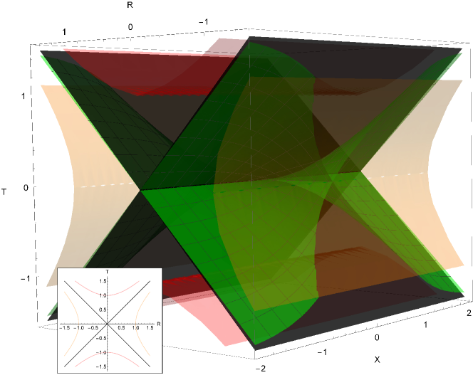
Figure 2: Kruskal diagram of the bulk spacetime. The black diagonal sheets correspond to the location of the black hole’s horizon. The red surfaces show the location of the singularity, and the orange surfaces show the location of the boundary at $z=0$. The green surface is the worldvolume of the bulk shockwaves along which the three regions of spacetime are glued together. A steady state region forms both for $t>0$ and for $t<0$. However, note that the physically relevant part of this spacetime for our investigation is assumed to be $t\geq 0$ only.

Focusing on the exterior of the black hole in figure 2, the shockwaves leave the central point $x=0$ at $t=0$. Therefore the initial location of the shockwave is marked by the horizontal ray $t=x=0,0\leq z\leq z_{H}$. Any other boundary point $x=x_{0}$ experiences the shockwave crossing at $t=|x_{0}|$ (and this extends radially all along $z$), so the location of the shockwave is marked by a straight line that increasingly separates from the initial horizontal line as $|x_{0}|$ increases. Gathering the locations corresponding to a shockwave for all values of $x$, we obtain the green surface in figure 2. This figure displays that in this causal diagram, the shockwave worldvolume does not touch the horizon surface, except at the line corresponding to $T=R=0$, which is the bifurcation surface. Consequently, the only part of the event horizon of the static regions on the left and on the right that is retained in this construction is a half of the bifurcation surface for each side. Apart from that, only the event horizon of the steady-state region appears, it remains untouched by the shockwaves on which the gluing of spacetimes takes place.

As mentioned above, the analysis of the causal diagram in figure 2 reveals another important aspect of the shockwaves: their spacelike nature, i.e. the fact that their induced metric will have positive determinant. Intuitively, this means that in the bulk, they would be perceived as being superluminal. Of course, this raises puzzling questions concerning whether this system should be considered to be physical or not. However, we note that the present geometry is a solution of vacuum in three dimensions, in which general relativity does not have propagating degrees of freedom. Therefore, these shockwaves do not transport information in the bulk, and every bulk observer will locally observe AdS space everywhere. However as we will see from the time dependence of entanglement entropy later on, from the dual CFT perspective the shockwaves, which travel at the speed of light on the boundary, do transport information. Considerations of energy conditions in the bulk are also unnecessary, given that it is a vacuum solution (including the fact that $S_{ij}=0$ in (17)), so most common energy conditions are trivially satisfied.

The intuitive picture of why information is not transported by these shockwaves in the bulk can be understood by taking into account that apparent faster than light propagation is present in many physical situations. In order to illustrate this point, we look at the example of two rulers, as in figure 3. The red dot corresponds to their point of intersection. As the rulers move in diverging directions (at speeds slower than light), as indicated by the arrows of the figure, their point of intersection moves forward at a higher speed. The velocity of this point depends on the angle between the two rulers, and it can move superluminally if the initial conditions conspire accordingly.

However, this point of intersection is an emergent object and not a physical one, so it does not carry information. As a consequence, causality is not violated. In other words, consecutive positions of that point are not causally related, even though the information about these events is encoded in the initial conditions. Similarly, the shockwaves of our system have dynamics encoded in the initial conditions and can develop apparent superluminal speeds, but since they do not carry information, causality is preserved.

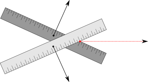
Figure 3: Two rulers moving at an angle. The red dot to the right indicates the point of intersection of the rulers. As the rulers move away in diverging directions, their point of intersection may move at superluminal speed, but without transport of information.

Another particular feature present in the $2+1$-dimensional case is that spacetime is always locally $AdS$, even at the matching surface. This means that a local observer traveling with the shockwave still sees $AdS$ everywhere. This is why the velocity and features of the shockwave cannot be physically relevant in the bulk.

In the following we holographically study the evolution of entanglement entropy in this setup. We find that it has physical behaviour in agreement with field-theory expectations. For instance, there is a well-defined velocity of propagation for entanglement entropy. This is in agreement with arguments using a quasiparticle picture Calabrese:2005in , according to which the initial condition acts as a source of pairs of quasiparticle excitations. As they propagate causally throughout the system, larger regions get entangled. In this picture, if a maximum quasiparticle velocity exists, then the entanglement entropy grows linearly in time for certain boundary regions. We will see that also holographically, there is a velocity associated to entanglement, independently of the gluing of the spacetimes. In fact, in the following section we will see that entanglement entropy does evolve in a causal manner, and obeys the velocity bound known from the study of entanglement tsunamis.

3 Numerical results I: Shooting method

We now turn to the numerical computation of entanglement entropy in the background introduced in the preceding section. For this purpose, we study minimal surfaces whose boundary at $z=0$ is in $x=x_{L}$ and $x=x_{R}$, and consider space-like intervals with $t(x_{L})=t(x_{R})$.  By the HRT prescription in $2+1$ dimensions Hubeny:2007xt , the minimal surface compatible with these boundary conditions corresponds to a geodesic in the bulk. This follows from a solution of the geodesic equations, which read

$$\frac{d^{2}x^{P}}{ds^{2}}+\Gamma^{P}_{MN}\frac{dx^{M}}{ds}\frac{dx^{N}}{ds}=0\,,\qquad P=t,x,z\,.$$ (19)

We assume an affine parametrization of the geodesic, which implies

$$\frac{\partial x^{M}}{\partial s}\frac{\partial x^{N}}{\partial s}g_{MN}=1\,.$$ (20)

The induced metric on the minimal surface reads

$$h_{ab}=\frac{\partial x^{M}}{\partial x^{a}}\frac{\partial x^{N}}{\partial x^{b}}g_{MN}=h_{ss}\,,$$ (21)

where $s$ is the coordinate of the surface. The entanglement entropy then follows from the area of the manifold $\gamma_{A}$, which can be computed from the induced metric as

$$S_{A}=\frac{1}{4G}\int_{s(x_{L})}^{s(x_{R})}ds\,{\cal L}\,,\qquad\textrm{with}\qquad{\cal L}=\sqrt{h_{ss}}\,.$$ (22)

From (20) and (21) we find that the entanglement entropy of (22) reduces to the trivial integral $S_{A}=\frac{1}{4G}\int_{s(x_{L})}^{s(x_{R})}ds$. The solution of the geodesic equations leads to the behavior $z\sim e^{-|s|}$ in the regime $s\to\pm\infty$. Consequently, the entanglement entropy is divergent. In the present case the divergence behaves as ${\textrm{Area}}(\gamma_{A}^{div})\sim-2L\log\epsilon+\cdots$, and a renormalization scheme is required. We use a minimal subtraction scheme, so that the renormalized entanglement entropy is defined as

$$S_{A}^{\textrm{ren}}=\frac{1}{4G}\left(\textrm{Area}(\gamma_{A})-\textrm{Area}(\gamma_{A}^{div})\right)\qquad\textrm{with}\qquad\textrm{Area}(\gamma_{A}^{div})=-2L\log\epsilon\,.$$ (23)

In the following we will compute renormalized entropies according to this formula.

3.1 Numerical solution of the geodesic equations

The geodesic equations of (19) consist of three coupled differential equations of second order, whose solution can be expressed in the parametric form

$$t=t(s)\,,\qquad x=x(s)\,,\qquad z=z(s)\,.$$ (24)

These equations can be solved by imposing six boundary conditions, which are

$$\begin{cases}t(s_{L})=t(s_{R})=t_{0}&\\ x(s_{L})=x_{L}\,,\qquad x(s_{R})=x_{R}&\\ z(s_{L})=z(s_{R})=\epsilon\,.&\end{cases}$$ (25)

We use the shooting method for the numerical computation of the geodesic equations: We shoot from $s=0$ with given values of $\{t(0),x(0),z(0)\}$ and $\{t^{\prime}(0),x^{\prime}(0),z^{\prime}(0)\}$, and then find the values of these initial conditions that lead to the desired boundary values at $s\to s_{L,R}$ given in (25). 

We introduce a cutoff $\epsilon\ll 1$ for regularization. This also induces a cutoff in the affine parameter, i.e. $s_{L}\sim-|\log\epsilon|$ and $s_{R}\sim|\log\epsilon|$. In the following we will consider space-like intervals $A$ and $B$ as shown in figure 4. Figures 5 and 6 display a typical solution of the geodesic equations, which satisfies the boundary conditions of (25). Once the geodesics are obtained, the next step is to compute the area of these curves and then the entanglement entropy from (23). We now present results for the time evolution of the entanglement entropy in the system of section 2.

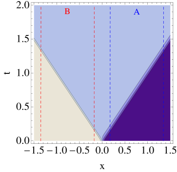
Figure 4: Contour plot of energy density $\langle T^{tt}(t,x)\rangle$ with the model in $d=2$, see section 2. Dashed lines show the time evolution of the endpoints of the intervals $A$ and $B$, in the positive and negative semiplane respectively. We consider the intervals $x^{A}\in[0.175,1.35]$ (blue) and $x^{B}\in[-1.35,-0.175]$ (red), temperatures $T_{L}=0.2$, $T_{R}=0.195$ and $\alpha=25$ (in equation (10)), in units in which $L=1$.

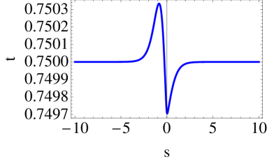
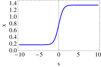
Figure 5: Parametric dependence of the geodesic as a function of the affine parameter $s$. We show $t=t(s)$ (left) and $x=x(s)$ (right). We have considered the interval $x^{A}\in[0.175,1.35]$ as shown in figure 4, and $t_{0}=0.75$, see equation (25).

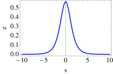
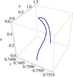
Figure 6: Parametric dependence of the geodesic. (Left) We show $z=z(s)$. (Right) Geodesic in the space $(t,x,z)$. See figure 5 for further details.

3.2 Entanglement entropy and universal time evolution

For the moment we consider a single interval $x\in[x_{L},x_{R}]$ denoted by $A$, placed in the positive semiplane, i.e. $x_{L,R}>0$. Let us study the time evolution of the entanglement entropy $S_{A}$ during the formation of the steady state. We are considering the model in $d=2$, so that the shockwaves are at $t=|x|$. This means that the shockwaves touch the two ends of the interval at times $t=|x_{L}|$ and $t=|x_{R}|$, see figure 4. We will denote these values by $t_{1}$ and $t_{2}$, respectively. In the limit $\alpha\to\infty$ in (13), the entanglement entropy turns out to be constant in the regimes $0\leq t\leq t_{1}$ and $t_{2}\leq t$, and there is a non-trivial time evolution only in the interval $t_{1}\leq t\leq t_{2}$, i.e.

$$S_{A}(t)=\begin{cases}S_{A}(t=0)&0\leq t\leq t_{1}\\ S_{A}(t)&t_{1}\leq t\leq t_{2}\\ S_{A}(t=\infty)&t_{2}\leq t\end{cases}\,.$$ (26)

We display in figure 7 (left) the time evolution of the entanglement entropy of interval $A$ of figure 4, from a numerical computation of the geodesic equations. In this and subsequent figures we display the entanglement entropy renormalized as shown in equation (23). Let us focus on the regime $t_{1}\leq t\leq t_{2}$. It is convenient to define the normalized entanglement entropy $f_{A}(\rho)$ as

$$f_{A}(\rho)\equiv\frac{S_{A}(t)-S_{A}(t=0)}{S_{A}(t=\infty)-S_{A}(t=0)}\qquad\textrm{with}\qquad\rho\equiv(t-t_{1})/\Delta t\,,$$ (27)

where $\Delta t=\ell=|x_{R}-x_{L}|$. This corresponds to the function $S_{A}(t)$ normalized to the interval [0,1] in both horizontal and vertical axes for $t_{1}\leq t\leq t_{2}$. It is clear from equations(26) and (27) that $f_{A}(\rho)$ has the values $f_{A}(0)=0$ and $f_{A}(1)=1$. We have computed numerically the entanglement entropy $S_{A}(t)$ in number of configurations with different temperatures $T_{L}$, $T_{R}$ and lengths $\ell$, and find that for a large range of temperature differences, the behavior of $f_{A}(\rho)$ may be approximated by

$$f_{A}(\rho)\simeq 3\rho^{2}-2\rho^{3}\,,\qquad 0\leq\rho\leq 1\,.$$ (28)

Specifically, this function fits extremely well the numerical results of the entanglement entropies as long as $\ell T_{L}<1$ and $\ell T_{R}<1$. This is illustrated in figure 7 (right) for a particular case. The result of equation (28) is independent of the values of the parameters $T_{L}$, $T_{R}$ and $\ell$, and so it implies the existence of an ’almost’ universal time-evolution of entanglement entropy in the theory with $d=2$ at small temperatures. Eq. (28) will be proven analytically in section 5.2 within a small temperature expansion.

The analysis presented above applies also to intervals in the negative semiplane. We show in figure 7 (left) the entanglement entropy of interval $B$ of figure 4. Note that both functions, $S_{A}(t)$ and $S_{B}(t)$, tend to the same value when the intervals reach the steady-state regime.

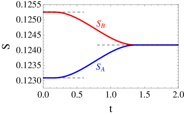
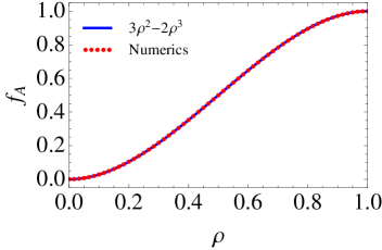
Figure 7: (Left) Renormalized entanglement entropies of intervals $A$ and $B$ as a function of time, see figure 4. The intervals correspond to $x^{A}\in[0.175,1.35]$ and $x^{B}\in[-1.35,-0.175]$, and temperatures $T_{L}=0.2$ and $T_{R}=0.195$. The (dashed) horizontal lines correspond to the results by using the analytical formulae (34) and (35). We have set $G=1$ and $L=1$. (Right) Renormalized entanglement entropy $S_{A}$ as a function of time, normalized to $[0,1]$ in both horizontal and vertical axes, see (27). The dots correspond to the numerical result with the interval $A$ in figure 4, while the continuous line is the universal behavior $f_{A}(\rho)=3\rho^{2}-2\rho^{3}$.

3.3 Time evolution of mutual information

A quantity of interest related to the entanglement entropy is the mutual information. It measures which information of subsystem $A$ is contained in subsystem $B$, or in other words the amount of information that can be obtained from one of the subsystems by looking at the other one. An advantage of this quantity is that it is finite, so that it does not need to be regularized. It is defined as

$$I(A,B)=S_{A}+S_{B}-S(A\,\cup B)\,,$$ (29)

where, holographically,

$$S(A\,\cup B)=\textrm{min}\bigg{\{}S_{A}+S_{B},S_{1}+S_{2}\bigg{\}}\,,$$ (30)

and $S_{1}$ and $S_{2}$ are defined as the entanglement entropy of the intervals $[x_{R}^{B},x^{A}_{L}]$ and $[x_{L}^{B},x^{A}_{R}]$ respectively, see figure 4. Note that the mutual information satisfies $I(A,B)\geq 0$. This corresponds to the simplest example of inequalities of entanglement entropies in a system involving a number of subsystems. See also section 6 for a further discussion.

We have numerically studied the time evolution of $S(A\,\cup B)$ and the mutual information $I(A,B)$. The results are shown in figure 8. An important property that we can infer from this result is that, contrary to the entanglement entropy $S_{A}$ or $S_{B}$, the mutual information always grows with time, i.e.

$$\partial_{t}I(A,B)\geq 0\,.$$ (31)

We have checked this property for a large number of configurations, with different temperatures and intervals, and it always remains valid. This seems to imply that in the boundary picture, the shockwaves transport information about the presence of the other heat bath throughout the system. Note that while the hypersurfaces describing the shockwave in the bulk are spacelike and can hence not carry information in the bulk picture (as explained in section 2), the shockwaves are null on the boundary, and hence they can be interpreted to transport information from the boundary perspective.

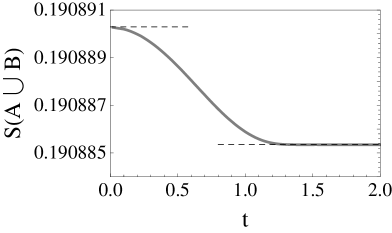
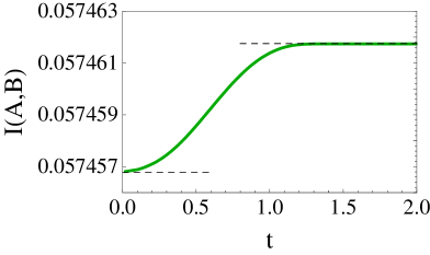
Figure 8: (Left) Renormalized entanglement entropy of $A\,\cup B$ as a function of time, see figure 4. (Right) Mutual information of $A$ and $B$ as a function of time. In these figures the (dashed) horizontal lines correspond to the results by using the analytical formulas, equations(33), (34) and (35). The intervals correspond to $x^{1}\in[-0.175,0.175]$ and $x^{2}\in[-1.35,1.35]$, and temperatures $T_{L}=0.2$ and $T_{R}=0.195$. We have set $G=1$ and $L=1$.

3.4 Conservation of entanglement entropy

Let us consider the two extreme regimes $t=0$ and $t\to\infty$. It is possible to obtain analytical results for the entanglement entropies in these cases for the model with $d=2$ presented in section 2. On the spacelike slice defined by $t=0$, the metric corresponds to two black holes of different temperature located to the left and right of $x=0$ each, i.e.

$$ds^{2}=ds_{L}^{2}\theta(-x)+ds_{R}^{2}\theta(x)\,,$$ (32)

and in this case the entanglement entropy for an interval $[x_{L},x_{R}]$ with $x_{L}<0$ and $x_{R}>0$ becomes, using minimal subtraction,

$$S(T_{L},x_{L};T_{R},x_{R})=$$ (33)

$$\qquad\qquad\frac{L}{2G}\log\left[\frac{T_{\mathrm{L}}\cosh\left(\pi T_{\mathrm{L}}x_{\mathrm{L}}\right)\sinh\left(\pi T_{\mathrm{R}}x_{\mathrm{R}}\right)-T_{\mathrm{R}}\sinh\left(\pi T_{\mathrm{L}}x_{\mathrm{L}}\right)\cosh\left(\pi T_{\mathrm{R}}x_{\mathrm{R}}\right)}{\pi T_{\mathrm{L}}T_{\mathrm{R}}}\right]\,.$$

To obtain this expression we considered the length of a curve piecewise defined in the two heat baths, consisting of two pieces at $x<0$ and $x>0$ glued together at $x=0$. They are parts of two geodesics, defined in a geometry with a black hole at temperature $T_{\mathrm{L}}$ and $T_{\mathrm{R}}$, respectively. The curve is chosen such that its length is minimal with respect to the value of the radial coordinate at which the two geodesics meet at $x=0$. For a similar matching-based method see section 4.

If we place the interval in just one semiplane, i.e. $x_{L,R}>0$ (or $x_{L,R}<0$), the entanglement entropy at $t=0$ corresponds to the one for a stationary black hole at temperature $T$, which reads

$$S(T,\ell;t=0)=\frac{L}{2G}\log\left(\frac{1}{\pi T}\sinh(\pi\ell T)\right)\,,\qquad\ell:=|x_{R}-x_{L}|\,.$$ (34)

In this equation $T=T_{L}$ (or $T_{R}$) when $x_{L,R}<0$ (or $x_{L,R}>0$). In the other extreme, $t\to\infty$, the system is in the steady-state regime, and the entanglement entropy is the one for a boosted black hole,

$$S(T_{L},T_{R},\ell;t=\infty)=\frac{L}{4G}\log\left(\frac{1}{\pi^{2}T_{L}T_{R}}\sinh\left(\pi\ell T_{L}\right)\sinh\left(\pi\ell T_{R}\right)\right)\,.$$ (35)

These analytical results, equations(34) and (35), correspond to $S_{A}(t=0)$ and $S_{A}(t=\infty)$ in equation (26), respectively. From these formulae we easily obtain the property

$$S_{A}(t=0)+S_{B}(t=0)=S_{A}(t=\infty)+S_{B}(t=\infty)\,,$$ (36)

where we consider intervals $A$ with $x^{A}_{L,R}>0$, and $B$ with $x^{B}_{L,R}<0$, and lengths $\ell=\ell_{A}=\ell_{B}$. This property is non-trivial, as in the left-hand side of equation (36) there is the contribution of stationary black hole solutions at temperatures $T_{L}$ and $T_{R}$, while in the right-hand side there is a boosted black hole and the corresponding energy flow contributes as well to the entanglement entropy. This relation is significant as it implies the ’conservation’ of entanglement entropies between $t=0$ and $t=\infty$. However, there is a non-trivial time evolution at intermediate times, as we discuss below. Interestingly, (36) has also been obtained in a slightly different setup in Hoogeveen:2014bqa .

In figure 9 (left), the time evolution of $S_{A+B}\equiv S_{A}+S_{B}$ is displayed. We see that our numerics confirm the conservation law of equation (36). In the next subsection we will study this system in the quenching regime, i.e. $t_{1}\leq t\leq t_{2}$ in equation (26), and characterize the violations of the entanglement entropy conservation in this case.

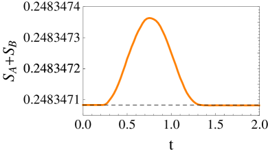
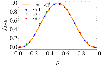
Figure 9: (Left) Renormalized entanglement entropy $S_{A}+S_{B}$ as a function of time, see figure 4. The (dashed) horizontal line corresponds to the result by using the analytical formulae (34) and (35). We have set $G=1$ and $L=1$. (Right) Renormalized entanglement entropy $S_{A+B}$ as a function of time, normalized to $[0,1]$ in both horizontal and vertical axes, see (37). The dots correspond to the numerical result with intervals $A$ and $B$, placed symmetrically with respect to $x=0$ as shown in figure 4, in different configurations: Set 1 is $(T_{L}=0.2,T_{R}=0.195,\ell_{A}=\ell_{B}=1.175)$, Set 2 is $(T_{L}=0.2,T_{R}=0.175,\ell_{A}=\ell_{B}=1.175)$ and Set 3 is $(T_{L}=0.2,T_{R}=0.175,\ell_{A}=\ell_{B}=1.475)$. The continuous line is the universal behavior $f_{A+B}(\rho)=\left[4\rho(1-\rho)\right]^{3}$.

3.5 Non-universal effects in time evolution

As it is shown in figure 9 (left), we find from our numerics that $S_{A+B}(t)\neq const$ in the quenching regime. This implies that the entanglement entropy is not conserved at intermediate times. A straightforward computation shows that these non-conservation effects are only possible if there are non-universal contributions in equation (28), otherwise this equation would predict $S_{A+B}(t)=const$.

In the following we restrict to intervals $A$ and $B$ with the same length and placed symmetrically with respect to $x=0$, i.e. $\ell_{A}=\ell_{B}$ and $x_{L,R}^{A}=-x_{R,L}^{B}$. While the function $S_{A+B}(t)$ has the same value at $t=0$ and $t=\infty$ (see (36)), we find from our numerics that it has a maximum at $t_{\textrm{max}}\approx(t_{1}+t_{2})/2$. In order to characterize the time evolution of $S_{A+B}(t)$, let us define the normalized entanglement entropy

$$f_{A+B}(\rho)\equiv\frac{S_{A+B}\left(t\right)-S_{A+B}(t=0)}{S_{A+B}(t_{\textrm{max}})-S_{A+B}(t=0)}\qquad\textrm{with}\qquad\rho\equiv(t-t_{1})/\Delta t\,,$$ (37)

where $t_{1}$ and $\Delta t$ are defined as in equation (27). Finally, from a numerical computation of $f_{A+B}(\rho)$ in a variety of intervals, we find that its behaviour is well-approximated by

$$f_{A+B}(\rho)\simeq\left[4\rho(1-\rho)\right]^{3}\,,\qquad 0\leq\rho\leq 1\,.$$ (38)

This is illustrated in figure 9 (right) for several configurations. From a combination of the results in (28) and (38), we conclude that for small temperatures, the normalized entanglement entropy defined in equation (27) can be approximated by

$$f_{A}(\rho)=3\rho^{2}-2\rho^{3}+\Delta_{A}(\rho)\,,\quad\textrm{with}\quad\Delta_{A}(\rho)\simeq C(T_{L},T_{R},\ell)\cdot[4\rho(1-\rho)]^{3}\,.$$ (39)

The factor $C(T_{L},T_{R},\ell)$ has a non-universal dependence on the parameters of the interval, so that $\Delta_{A}(\rho)$ is a non-universal contribution to $f_{A}(\rho)$. Note, however, that $C(T_{L},T_{R},\ell)$ does not appear to affect the universal behavior of $f_{A+B}(\rho)$, see (38). Some remarks deserve to be mentioned: On the one hand, $\Delta_{A}(\rho)$ is a correction of order ${\cal O}(\rho^{3})$, so that it does not jeopardize the early-time behavior $S_{A}(t)\sim t^{2}$ which is present in a wide variety of systems, see e.g. Balasubramanian:2010ce ; Balasubramanian:2011ur ; Balasubramanian:2011at ; Hartman:2013qma ; Liu:2013iza ; Li:2013sia ; Liu:2013qca ; Kundu:2016cgh ; OBannon:2016exv ; Lokhande:2017jik . On the other hand, the effect of $\Delta_{A}(\rho)$ is extremely small in the configurations we studied numerically. The range of validity of equation (28) will be further discussed in sections 4 and 5.

4 Numerical results II: Matching of geodesics

This section is devoted to an approach complementary to solving the geodesic equation as above – a method that we refer to as the matching approach. The idea is rather simple and based on the same principle as the variational derivation of the light refraction law. In short: we take the discontinuous shockwave geometry, where the metric is piecewise constant and coincides either with the standard or the boosted Schwarzschild metric. We calculate geodesics in each of these two spacetime regions and parametrize them by the positions of two points: One of these is located where the geodesic meets the conformal boundary of AdS, and the other where the geodesic meets the shockwave. We take two geodesics that reach the shockwave at the same point, each of them being located in one of the two regions of spacetime. We add their (renormalised) lengths and extremise the sum with respect to the position of the ’meeting point’ at the shockwave. The value of the length at the extremum yields the desired entanglement entropy of an interval enclosed by the ’boundary’ endpoints of our geodesics. Having painted the procedure by a broad brush, we shall now describe some technical details and assumptions made to carry out this procedure.

4.1 Setup and assumptions

Let us take the metric in its piecewise form (15, 16). The metric is a piecewise smooth function of Fefferman-Graham coordinates, denoted by $\tilde{z},\tilde{t},\tilde{x}$ in this section. We use the name region to refer to the whole subset of our space on which the metric coefficients are smooth, e.g steady state region (denoted $S_{\text{\ss}}$) is given by $\tilde{t}>0,~{}|\tilde{x}|<\tilde{t},~{}\tilde{z}\in\left(0,(\pi{}\sqrt{T_{L}T_{R}})^{-1}\right)$. In the same manner, the left and right thermal regions will be denoted by $L$ and $R$, respectively. The dimension two surface along which the metric is discontinuous will be referred to as the shockwave. Our aim is to calculate (regularised) geodesics length between two points lying on the conformal boundary of the space-time. If both endpoints belong to the same region, the answer is already known to be (5) in a thermal region and (8) in the steady state region. If, however, the boundary points belong to different regions, finding the solution is a more complicated task. We therefore make some assumptions about the spacetime.
Most importantly, we assume that the coordinates $\tilde{z},\tilde{t},\tilde{x}$ cover all the regions in a smooth way, and it is actually the metric components as functions of $\tilde{z},\tilde{t},\tilde{x}$ that are discontinuous. This assumption can be motivated by the fact that our metric (15, 16) can be obtained as a limit of a continuous metric (11, 13) where the shockwave width ($w$) tends to zero ($\alpha$ goes to infinity). It is reasonable to assume that taking the limit described does not influence the domain of our coordinates. The agreement between numerical results from the continuous model at large $\alpha$ and the results of this section shall confirm that the assumption made yields correct results. From the assumption follows in particular that curves which are continuous in our coordinates are also continuous on the manifold itself. This will be essential in our calculation, since it is based on joining two smooth curves in a way that it is still continuous.

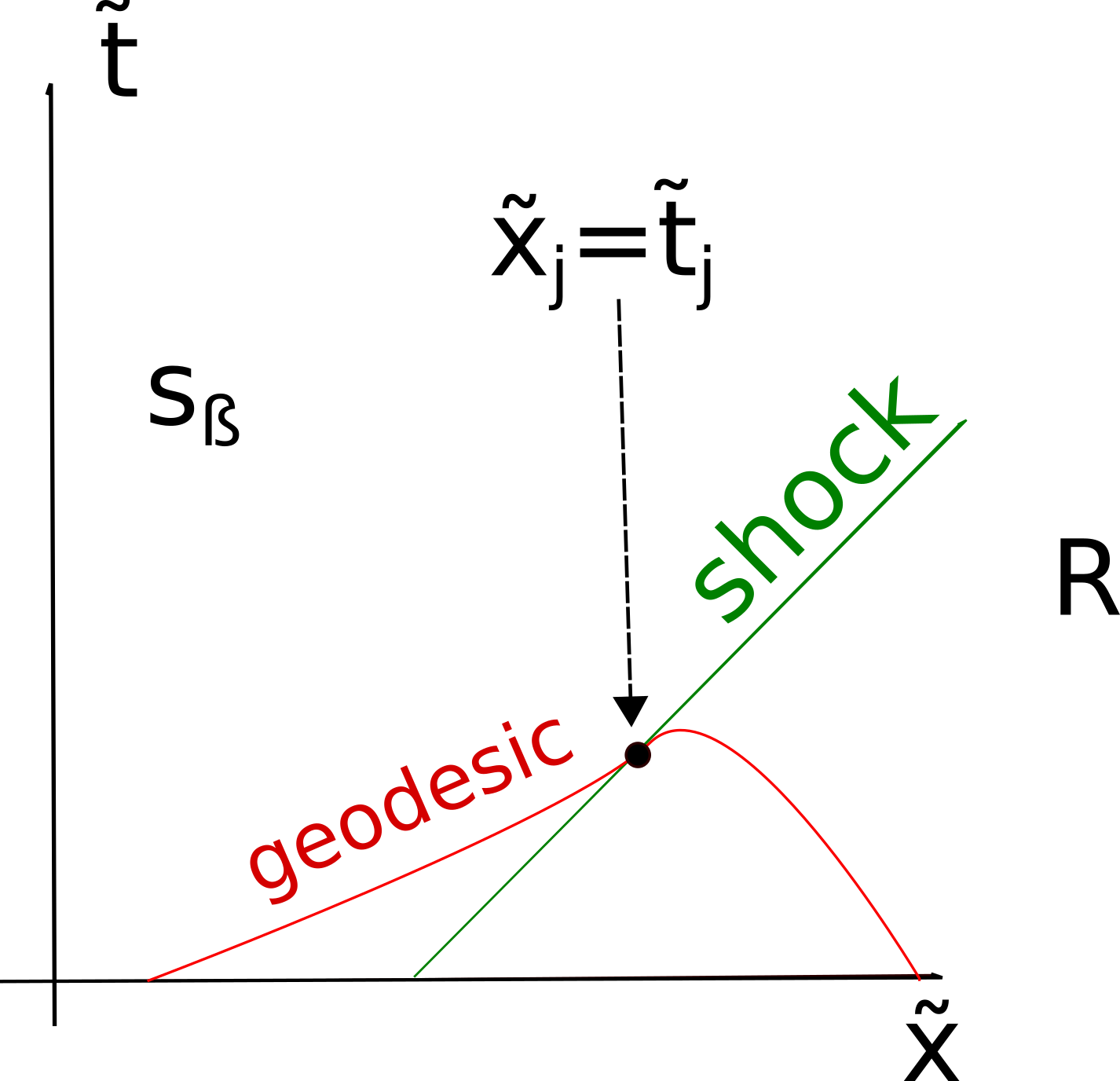
Figure 10: A cartoon of a curve used in our procedure, projected onto a $\tilde{t},x$ hypersurface. $S_{\text{\ss}}$ and $R$ denote regions of spacetime, the steady state and right thermal region, respectively. The red line is a piecewise geodesic (it is a geodesic in any of both regions) connecting boundary endpoints and a point on a shockwave ($\tilde{x}=\tilde{t}$ in our coordinates). Then the (renormalised) length of that geodesic is extremised with respect to the coordinates of the joining point, which yields the entanglement entropy.

4.2 Geodesics and distance

Given our setup, we need to calculate a spacelike distance between a given point on the boundary and an arbitrary point on the shockwave. To achieve this, we shall follow the logic of Shenker:2013pqa and utilise the fact that every three-dimensional asymptotically AdS manifold that is a solution to Einstein’s equations is locally isometric to AdS₃. So, if we identify the isometry, we may use the ready formulæ for geodesic distance in AdS₃ space. It is worth noting that thanks to this property special to three dimensions, we do not need to calculate the geodesics explicitly, we just express their length as a function of coordinates of the two points. This considerably simplifies the calculation. However, we still have to find formulæ for the geodesic distance in our problem. The metric (15, 16) is given in Fefferman-Graham (FG) coordinates. To use the results of Shenker:2013pqa , we need to change to Schwarzschild-type coordinates. There is a technical difficulty in that step: in every region the change of coordinates takes a different form. We denote FG-type coordinates as $(\tilde{z},~{}\tilde{t},~{}\tilde{x})$ and the Schwarzschild coordinates as $(z,~{}t,~{}x)$. In Schwarzschild coordinates, the metric takes the form (3)

$$\mathrm{d}s^{2}=\frac{L^{2}}{z^{2}}\left[-\left(1-(2\pi Tz)^{2}\right)\mathrm{d}t^{2}+\frac{\mathrm{d}z^{2}}{1-(2\pi Tz)^{2}}+\mathrm{d}x^{2}\right]\,,$$ (41)

where $T$ is a real, positive constant – an (effective) temperature. Then, the coordinate transformations are obtained as follows. For the steady state they read

$$z =\frac{\tilde{z}}{1+\pi^{2}T_{L}T_{R}\tilde{z}^{2}},$$ (42)

$$\tilde{z} =\frac{1-\sqrt{1-4\pi^{2}T_{L}T_{R}z^{2}}}{2\pi^{2}T_{L}T_{R}z},$$ (43)

$$\left(\begin{array}[]{c}t\\ x\end{array}\right) =\left(\begin{array}[]{c c}\cosh\left[\theta\right]&-\sinh\left[\theta\right]\\ -\sinh\left[\theta\right]&\cosh\left[\theta\right]\end{array}\right)\left(\begin{array}[]{c}\tilde{t}\\ \tilde{x}\end{array}\right),$$ (50)

$$\sinh\left[\theta\right] =\frac{T_{L}-T_{R}}{2\sqrt{T_{L}T_{R}}},~{}\cosh\left[\theta\right]=\frac{T_{L}+T_{R}}{2\sqrt{T_{L}T_{R}}}.$$

(42) is the inverse relation to (43). We quote both since there is a sign to be fixed. From (50) it follows that the effective temperature from equation (41) for the steady state can be expressed in terms of the reservoirs’ temperatures as

$$T=\sqrt{T_{L}T_{R}}.$$ (51)

For the thermal regions it is sufficient to take (42) and set $T_{L}=T_{R}$, $\theta=0$ to obtain

$$\tilde{z}=\frac{1-\sqrt{1-4\pi^{2}z^{2}T_{L/R}^{2}}}{2\pi^{2}T_{L/R}^{2}z}.$$ (52)

The distance can be expressed, following Shenker:2013pqa , as

$$\cosh\left[\frac{d}{L}\right]=T_{1}T_{1}^{\prime}+T_{2}T_{2}^{\prime}-X_{1}X_{1}^{\prime}-X_{2}X_{2}^{\prime}$$ (53)

with $d$ the geodesic distance. In terms of the Schwarzschild coordinates, the functions $X_{1},~{}X_{2},~{}T_{1},$ and $T_{2}$ read

$$T_{1} =\frac{z_{H}\sqrt{1-\frac{z^{2}}{z_{H}^{2}}}\sinh\left(\frac{t}{z_{H}}\right)}{z},$$ (54)

$$T_{2} =\frac{z_{H}\cosh\left(\frac{x}{z_{H}}\right)}{z},$$ (55)

$$X_{1} =\frac{z_{H}\sqrt{1-\frac{z^{2}}{z_{H}^{2}}}\cosh\left(\frac{t}{z_{H}}\right)}{z},$$ (56)

$$X_{2} =\frac{z_{H}\sinh\left(\frac{x}{z_{H}}\right)}{z},$$ (57)

with Schwarzschild horizon radius $z_{H}=(2\pi T)^{-1}$. From the formulae above it is clear that if one of the points is taken to the boundary ($z=0$) while the other is being kept fixed, the distance must diverge. Therefore, a regularisation is needed for small $z$. Since from (42) and (52) it follows that in every region

$$z=\tilde{z}+\mathcal{O}(\tilde{z}^{3}),$$

there is no difference in which coordinates we regularise. For concreteness, let us sketch the procedure of computing the regularised length for a case in which one end of the geodesic reaches the boundary in the steady state region and the other in the right thermal region with temperature $T_{R}$ (that is the case of figure (10)). So, we are interested in two lengths: one for the curve connecting the ‘starting point’ on the boundary ($\tilde{t}_{b},~{}\tilde{x}_{min},~{}z=\epsilon{}$) with a point on the shockwave $\tilde{x_{j}},~{}\tilde{x_{j}},~{}\tilde{z}_{j}$ and another joining the same point on a shockwave with the endpoint on a boundary on another side ($\tilde{t}_{b},~{}\tilde{x}_{max},z=\epsilon{}$), and then take a ’regularised limit’ $\epsilon\rightarrow 0$ (i.e. subtracting the divergent part and then taking the limit). To apply (53), we need to connect these to the Schwarzschild coordinates of the respective patches. Let us note that the condition for the position of the shockwave is identical in any of the used coordinates,

$$x_{j}=t_{j}\Leftrightarrow\tilde{x}_{j}=\tilde{t}_{j}.$$

For simplicity, we regularise in Schwarzschild coordinates. Using the asymptotic approximation of hyperbolic cosine by an exponential, we arrive at the conclusion that the minimal counter-term used in (23) is indeed the proper one to regularise our length. At this point it is convenient to set the $\text{AdS}_{3}$  radius to unity, $L=1$.
Now, we are ready to write the full, renormalised distance as a function of the joining point on the shockwave,

$$d_{R}(z_{j},x)= \log\left[\left(1+\pi^{2}T_{R}^{2}\tilde{z}_{j}^{2}\right)\cosh\left({2\pi T_{R}(x-\ell)}\right)-(1-(\pi T_{R}\tilde{z}_{j})^{2})\cosh\left({2\pi T_{R}(t-x)}\right)\right]+$$

$$\log\Big{[}\left(1+\pi^{2}T_{L}T_{R}\tilde{z}_{j}^{2}\right)\cosh\left({\pi(tT_{L}-tT_{R}+2T_{R}x)}\right)$$ (58)

$$+\left(\pi^{2}T_{L}T_{R}\tilde{z}_{j}^{2}-1\right)\cosh\left({\pi(t(T_{L}+T_{R})-2T_{R}x)}\right)\Big{]}-\frac{1}{2}\log\left(16\pi^{8}T_{L}^{2}T_{R}^{6}\tilde{z}_{j}^{4}\right).$$

In the above, we used a shortened notation: $\ell=\tilde{x}_{max}-\tilde{x}_{min}$, $x=\tilde{x}_{j}-\tilde{x}_{min}$, $t=\tilde{t}_{b}-\tilde{x}_{min}$ – the time that has passed since the shockwave entered the boundary interval. Now, this quantity is to be extremised with respect to, $\tilde{z}_{j}$ and $x$ (which is the same as extremising w.r.t $\tilde{x}_{j}$). Extremal points are solutions to

$$\partial_{\tilde{z}_{j}}d_{R}=0\,,\qquad\partial_{x}d_{R}=0\,.$$ (59)

These equations turn out to be fourth order polynomial equations in $z_{j}$ and non-polynomial equations in $x$. Therefore, we turn to numerical methods for solving non-linear algebraic equations. Note however that the above-mentioned system can be solved analytically in certain simplifying cases, see section 5. Upon solving the system (59), we obtain the coordinates of the extremum of $d_{R}$, namely ($z_{0},~{}x_{0}$). Then the desired entanglement entropy is given by

$$S=\frac{1}{4}d_{R}(z_{0},x_{0}).$$ (60)

4.3 Numerical algorithm

To solve the non-linear algebraic system (59), we need to involve numerical analysis. Our solution was developed in Wolfram Mathematica. All the codes used in this section are available online as supplementary material to the arXiv submission of the paper. The algorithm consists of two steps: First, following the idea of wagon2010mathematica in a slightly modified form (see GraphAnalysi ), we find a rough approximation of the solution by plotting curves satisfying each of the two equations in (59). Then we use coordinates of crossing points of those as a starting point for standard Newton’s solver built-in Mathematica’s FindRoot function. To understand why such a two-step procedure is necessary, let us briefly discuss the function (58) and equations (59).

Figure 11: The distance function $d_{R}(z_{j},x_{j})$ for parameters: $t_{b}=0.7,~{}x_{min}=0.5,~{}x_{max}=1.5,~{}T_{L}=2,T_{R}=1$ in units where $L=1$. The function turns imaginary outside of some region (where the argument of the logarithm in (58) turns negative).

As figure 11 shows, the domain of the distance function and the the full domain of our coordinates are not the same. This is in agreement with the fact that on a Lorentzian manifold, not every point is spacelike-separated from a given point. Then, the function going to zero and ceasing to be real signals that one of the boundary endpoints becomes null or time-like separated from the joining point. However, since $d_{R}=\log(...)$, both equations (59) have the form $\partial\log(f(...))=0$, so looking for their solution is equivalent to solving $\partial f(...)=0$ if $f$ does not vanish on the solution. This equivalent form is strongly preferable, given the nature of the numerical computations, in which unnecessary divisions decrease numerical precision. On the other hand, the modified system of equations consists of two functions that are well-defined for the whole domain of our coordinates. Therefore, we begin our numerical approach with an algorithm capable of finding rough approximations of all solutions to the system of equations in a given domain. From those solutions we choose the ones satisfying our requirement that the length evaluated on solution is positive. Then, these solutions are refined by using Newton’s method that yields the solution with the desired accuracy, in our case fifteen digits. If more than one solution is regular in the sense that the length is positive, the final answer is taken to be the one for which the value of length is smallest, according to the HRT proposal. The domain in which we search for solutions is (in terms of variables defined in (58))

$$x\in[0;L],~{}\tilde{z}_{j}\in[0;1.0001*(\pi\sqrt{T_{L}T_{R}})^{-1}]$$ (61)

on the left side, or

$$x\in[0;L],~{}\tilde{z}_{j}\in[0;1.0001*(\pi T_{L})^{-1}]$$ (62)

on the right, which ensures that solutions lying far below the horizon are excluded. This however allows the algorithm to look for the solution arbitrarily close to the horizon, and to boost the data generation.

To justify the exclusion of solutions with $\tilde{z}_{j}>\tilde{z}_{H}$, we have numerically tested that the solutions lying below the horizon, should they appear, are not the physical ones. The argument behind this is based on the analysis of the Kruskal diagram of our space-time (see figure 2). In short, we see that the shockwave does not cross the horizon except for the bifurcation surface – it stays entirely in the outer region of the black hole. This means that the point where the geodesic crosses the shockwave will generically be outside of the horizon ($\tilde{z}<\tilde{z}_{H}$), and since this is a causality argument, this occurs both from the point of view of the static region and from the point of view of the steady state region. Indeed, we find that a solution to our matching equations with these properties always seems to exist. Therefore, the fact that we can find a solution beneath the horizon ($\tilde{z}_{j}>\tilde{z}_{H}$) is only an artefact of our choice of coordinates. On the numerical side we allow, for test purposes, $\tilde{z}_{j}$ to exceed the above mentioned bounds by large values ($2-3$ times larger), and the solutions found in those regions were never chosen by the algorithm. With the restricted domain of interest and given accuracy, our algorithm has an acceptable speed: computing the entanglement entropy for a given interval and a given boundary time takes roughly $0.2$ seconds.

4.4 Results

In this way we obtain entanglement entropy for a wide range of temperatures. To compare with results of the previous section, we consider properties of entanglement entropy of the same boundary regions, namely

$$A=[0.175,1.35],~{}B=[-1.35,-0.175].$$ (63)

All our data is generated using $\text{AdS}_{3}$  radius as unit, $L=1$. We are also going to take various temperature differences. In that subsection by $t$ we denote the boundary time, to stick to the conventions of the previous section. The first result, shown in figure 12, indicates that both our methods (of this and the preceding section) yield the same results for the same initial data. That ensures us about the correctness of our results, as numerical techniques used in both approaches are substantially different.

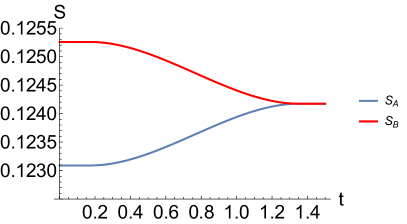
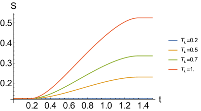
Figure 12: Comparison of entanglement entropies for intervals $A$ and $B$ at temperatures $T_{L}=0.2$ $T_{R}=0.195$ (left panel), and entanglement entropies for the interval $A$ in different temperatures – with $T_{R}=0.195$ and $T_{L}$ ranging from $0.2$ (blue curve) to $1.$ (orange) as functions of boundary time $t$. The left panel shows exact matching with previous results from figure 7, which is a consistency check. The right panel shows how the evolution changes when one gradually increases the temperature of one of the heat baths. All lengths in units of $\text{AdS}_{3}$  radius ($L=1$).

Now, let us analyse the universal formula for normalised entanglement entropy (27). Using the joining method we are not only able to prove the universal formula (see section 5), but also find in what range it is broken. The results on the universal formula for $f_{A}$ can be seen on figure 13.

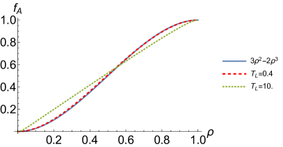
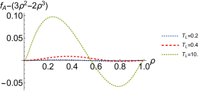
Figure 13: Normalised entanglement entropy $f_{A}$ for the interval $A$ in temperatures $T_{L}=0.4$ and $T_{L}=10.$ compared to the universal formula $3\rho^{2}-2\rho^{3}$ (left panel) and deviations from universal formula for $T_{L}=0.2,~{}0.4,~{}10.$ (right panel) The $T_{L}=0.2$ case was already shown on figure 13. In that case the deviation is approximately $0.002$. Upon increasing the temperature of the left bath, the deviation from the universal formula grows and the time evolution resembles more a straight line – however the difference $f_{A}(t)-t$ still reaches values around $0.04$ for $T_{L}=10.$. See section 5.4 for a discussion of the high temperature linear behaviour. All lengths in units of $\text{AdS}_{3}$ radius ($L=1$).

Finally, we reconsider the question of non-conservation of the sum $S_{A}+S_{B}$ with the alternative numerical approach of ths section. The results of figure 9 pass convergence tests, however the peak is tiny compared to the value of entropy (difference in 6-th decimal). Here we confirm the observed behaviour of $S_{A}+S_{B}$ in the alternative numerical approach. Our findings are presented on figure 14. An interesting fact is that we numerically find that the normalised sum

$$\frac{S_{A}(t)+S_{B}(t)}{2S_{A}(\infty)}$$ (64)

is bounded from above by a value of approximately $1.025$. So, the maximal deviation from a constant appears to be at most 2.5% of the value of entropy –which is however too much to attribute it to a numerical error.

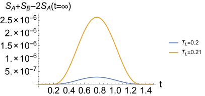
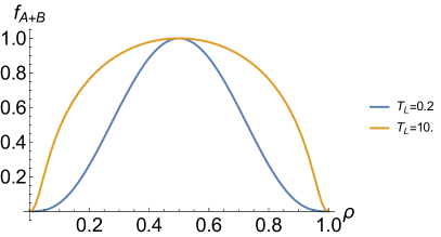
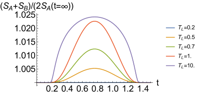
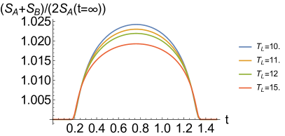
Figure 14: Top left: Sum of $S_{A}$ and $S_{B}$ for two different, yet close, values of $T_{L}$, shifted by the asymptotic ($t=\infty$) value of that sum. The blue plot is the case studied in section 3, as previously the deviation from constancy is of order $10^{-7}$ while the sum is of order $10^{-1}$. The yellow plot shows a similar quantity for temperature $T_{L}=0.21$, just slightly higher. The deviation is now order of magnitude bigger. Top right: Normalised deviation $f_{A+B}$ for different temperatures $T_{L}$. The blue curve has been already shown in figure 9 to follow the universal behaviour $[4\rho(1-\rho)]^{3}$. For much bigger temperature $T_{L}=10$, the shape of the curve changes considerably. Bottom: Ratio of sum $S_{A}+S_{B}$ and asymptotic value of that sum as a function of boundary time. The deviation of the sum from its asymptotic value reaches around $2.5\%$, but seems to be bounded even when one increases the temperature – compare left and right figures which are in the same scale. The bigger the temperature difference, the more the curve resembles a semi-circle. All lengths in units of $\text{AdS}_{3}$  radius ($L=1$).

5 Analytical results

Some of the numerical results presented in the two preceding sections may actually be obtained analytically, at least in some limits. This applies in particular to the result (28) for the time evolution of the entanglement entropy. Moreover, we derive a bound on the increase rate for the entanglement entropy. We begin this section in 5.1 by a review of velocity bounds previously obtained for global quenches. We then obtain analytical results for the time evolution of the entanglement entropy for the limit of both heat bath temperatures small in section 5.2 , and of one of the two temperatures vanishing in section 5.3. Finally we obtain a velocity bound on entanglement growth in section 5.4.

5.1 Review of universal velocity bounds

In the past, much interest has been directed towards the holographic study of the time dependent behaviour of entanglement entropy after global quenches. For example, in a series of papers AbajoArrastia:2010yt ; Balasubramanian:2010ce ; Balasubramanian:2011ur ; Balasubramanian:2011at ; Hartman:2013qma ; Liu:2013iza ; Li:2013sia ; Liu:2013qca , it was found that after a global quench, the entanglement entropy of a sufficiently large boundary region would exhibit an initial quadratic growth of entanglement with time,

$$\Delta S(t)\propto t^{2}+...,$$ (65)

followed by a universal linear growth regime where

$$\Delta S(t)=v_{E}s_{eq}A_{\Sigma}t+...\ .$$ (66)

In this formula, $t$ is the time after the quench, $\Delta S$ is the change in entanglement entropy, $s_{eq}$ is the entropy density of the (late time) equilibrium thermal state, $A_{\Sigma}$ is the surface area of the boundary region $\Sigma$ of which the entanglement entropy is computed and $v_{E}$ is a velocity that depends on the final equilibrium state. In the case of an AdS-Schwarzschild black hole as final state, it was found that AbajoArrastia:2010yt ; Liu:2013iza ; Li:2013sia ; Liu:2013qca

$$v_{E}=\frac{\sqrt{d}(d-2)^{\frac{1}{2}-\frac{1}{d}}}{\left(2(d-1)\right)^{1-\frac{1}{d}}},$$ (67)

which is referred to as the entanglement velocity or tsunami velocity. The reason for this nomenclature is that the behaviour (66) can be understood in terms of a heuristic picture in which the entanglement growth is caused by entangled quasi-particles that were created by the global quench and are propagating at the speed (67), forming the entanglement tsunami. See also Bai:2014tla ; Leichenauer:2015xra ; Ziogas:2015aja ; Tanhayi:2015cax ; Hartman:2015apr ; Casini:2015zua ; Mezei:2016zxg ; Mezei:2016wfz for further work on this topic. A related concept is the so-called butterfly velocity Shenker:2013pqa ; Roberts:2014isa

$$v_{B}=\sqrt{\frac{d}{2(d-1)}}$$ (68)

for the spatial propagation of chaotic behaviour in the boundary theory. This speed is also connected to the growth of operators in a thermal state Shenker:2013pqa ; Roberts:2014isa . From (67) and (68), it is obvious that

$$1\geq v_{B}\geq v_{E},$$ (69)

and the case $d=2$ is the special case where $1=v_{B}=v_{E}$. Interestingly, the velocities seem to play an important role in the description of entanglement spreading not only for global quenches, but also for local quenches Rangamani:2015agy ; Astaneh:2014fga ; Rozali:2017bco .

5.2 Time evolution of entanglement entropy: Both temperatures small

Based on the matching procedure outlined in section 4, it is easy to prove the universal formula (28) for the time evolution of entanglement entropy as an approximation for small $T_{L}$ and $T_{R}$. In order to do so, we simply replace $T_{L}\rightarrow\delta\cdot T_{L}$, $T_{R}\rightarrow\delta\cdot T_{R}$ and expand the expressions for $\partial_{z_{j}}d_{R}$ and $\partial_{x}d_{R}$ in (59) in the small quantity $\delta$. Similarly, we expand the analogous function $d_{L}$ and its derivative when $x_{max}\leq 0$. To lowest non-trivial order in $\delta$, we find

$$\partial_{x}d_{R}\propto\partial_{z_{j}}d_{L}\propto(\ell-t)(\ell+2t-4x)t-(\ell-2t)z_{j}^{2},$$ (70)

$$\partial_{z_{j}}d_{R}\propto\partial_{x}d_{L}\propto(\ell-t)(t-2x)(\ell+t-2x)t+z_{j}^{4}.$$ (71)

The condition $\partial_{z_{j}}d_{R}=\partial_{x}d_{R}=0$ (respectively $\partial_{z_{j}}d_{L}=\partial_{x}d_{L}=0$) has then the simple solution

$$x=t,z_{j}=\sqrt{(\ell-t)t}.$$ (72)

This may be inserted into $d_{R}$ in equation (58) and the similar expression for $d_{L}$, giving the entanglement entropy $S(t)$, and this in turn can be inserted into (27). Expanding again in small $\delta$ as above, we then find for both the left- and right-side the analytic result

$$f(\rho)=3\rho^{2}-2\rho^{3}$$ (73)

at order $\delta^{0}$. Here, $\rho$ is again the rescaled time defined in (27). It is interesting to note that the small $T_{L},T_{R}$ expansions leading to (73) loose their analytic validity at an order of magnitude of $T_{L},T_{R}$ at which our numerics are still well approximated by (73). It might hence be interesting to do the $T_{L},T_{R}$ expansions in a more systematic way and to study the higher orders in more detail. This might also help to understand the range of validity of equation (39).

It is worth stressing that the universal dynamics of entanglement entropy is not only of purely academic interest. It is known that the low-energy spectrum of excitations of some models (i.e systems with ballistic conductance, possessing quasiparticle description, see Bernard:2016nci ) are governed by effectively conformal theories. The regime in which this approximation is valid for thermal states is indeed when both of the temperatures are low, so the highest lying parts of spectrum are not largely populated in the thermal state – which is also the range of validity of our universal formula (28). This means that in the limit of small temperatures our universal evolution of entanglement entropy should be also valid in ballistic regimes of real, i.e electronic systems. It is therefore an interesting possible direction of investigation to compute other quantities, as correlation functions, in this low-temperature limit and compare them against expectations from other theories (i.e. lattice models).

5.3 Entanglement Entropy: Limit of zero temperature for one of the heat baths

In addition to the case where both temperatures $T_{L}$ and $T_{R}$ are small (studied in section 5.2), there is another situation where the matching equations derived in section 4 can be solved analytically: The case where $T_{R}=0$ with arbitrary $T_{L}$ (or the analogous case $T_{L}=0$ with arbitrary $T_{R}$, which we will not consider separately).

First of all, let us reassure ourselves that this case is actually physical. Setting $T_{R}\rightarrow 0$ in equations (140)-(144) has the consequences

$$T \rightarrow 0$$ (74)

$$\chi \rightarrow+\infty$$ (75)

$$\beta \rightarrow+1$$ (76)

$$\theta \rightarrow+\infty.$$ (77)

Despite the divergence of the rapidity $\theta$, we see that for $d=2$, the line element (6) of the boosted black hole has a well-defined limit

$$ds^{2} \rightarrow\frac{L^{2}}{z^{2}}\left(dz^{2}+(-1+\pi^{2}T_{L}^{2}z^{2})dt^{2}+(1+\pi^{2}T_{L}^{2}z^{2})dx^{2}-2\pi^{2}T_{L}^{2}z^{2}dtdx\right).$$ (78)

Similarly, instead of (58), we find the expression

$$d_{R}(z_{j},x)= \log\Big{[}4\pi^{3}\left(\ell^{2}-2\ell x-t^{2}+2tx+z_{j}^{2}\right)$$

$$\times\left(\pi T_{L}z_{j}^{2}\cosh\left(\pi tT_{L}\right)-(t-2x)\sinh\left(\pi tT_{L}\right)\right)\Big{]}$$ (79)

$$-\frac{1}{2}\log\left(16\pi^{8}T_{L}^{2}z_{j}^{4}\right)$$

which can be shown to be extremised for

$$x=\frac{\pi tT_{L}(\ell-t)\coth\left(\pi tT_{L}\right)+\ell+t}{2+2\pi T_{L}(\ell-t)\coth\left(\pi tT_{L}\right)},\ z_{j}=\sqrt{\frac{\ell(\ell-t)}{1+\pi T_{L}(\ell-t)\coth\left(\pi tT_{L}\right)}}.$$ (80)

This yields the analytic solution

$$S(\ell)\propto\log\left(\ell\sinh\left(\pi tT_{L}\right)\right)+\log\left(1+\pi T_{L}(\ell-t)\coth\left(\pi tT_{L}\right)\right)-\log(\pi T_{L}).$$ (81)

Expanding around $T_{L}=0$ yields to lowest order the universal formula (28) again, however (81) is an analytical result for the entanglement entropy which is valid for any $T_{L}$. For large $T_{L}$, we obtain

$$S(\ell)\approx\frac{L}{4G}\pi tT_{L}=s_{eq}t,$$ (82)

where we have used (85) with $T_{R}\equiv 0$. This result shows that for large $T_{L}$, the entanglement entropy will increase in an approximately linear way, saturating the bound to be discussed in section 5.4. Note the discrepancy of a factor $A_{\Sigma}=2$ between (82) and equation (66) for $d=2$, where $v_{E}=1$. This may be because in a global quench, the entanglement tsunami enters the interval of interest from both sides, while in our local quench like setup, the shockwave enters the interval only from one side. However, we should stress that in contrast to the entanglement tsunamis studied in global quenches in AbajoArrastia:2010yt ; Hartman:2013qma ; Liu:2013iza ; Li:2013sia ; Liu:2013qca ; Bai:2014tla ; Leichenauer:2015xra ; Ziogas:2015aja ; Tanhayi:2015cax ; Hartman:2015apr ; Casini:2015zua ; Mezei:2016zxg ; Mezei:2016wfz , we do not have a heuristic quasi-particle like picture explaining the entropy increase and decrease experienced by different intervals in our inhomogeneous setup even qualitatively. We will discuss the possible bounds on the entropy increase or decrease rate of different intervals in our system for general $T_{L},T_{R}$ in section 5.4.

5.4 Bounds on entropy increase rate

As shown in section 3, for the full time-dependent background (10) we expect that for an interval of length $\ell$, the time dependent entanglement entropy $S(\ell,t)$ will be constant before the shockwave enters the interval, evolve with time $t$ while the shockwave passes through the interval, and be constant again after the shockwave has left the interval. This is precisely the behaviour seen in figure 7, for example. Furthermore, normalising the entropy such as to obtain a dimensionless quantity, we have observed in section 3 that for small temperatures $T_{L},T_{R}$, the time dependence of the entanglement entropy can be approximated by the formula (28), which we analytically proved in section 5.2. In this section, we will have a closer look at the rates of entropy increase that we observe in the time dependent entanglement entropies $S(\ell,t)$.

We begin by analytically deriving some useful expressions. For a sharp shockwave moving at the speed of light, the change in the entanglement entropy of an interval with length $\ell$ will occur over a time period $\Delta t=\ell$. From (8) and (5) (with $T\rightarrow T_{L}$ for example, as appropriate when the interval is entirely on the left) we then easily find the average entropy increase rate

$$v_{av}\equiv\frac{\Delta S}{\Delta t}=\frac{L}{4G\ell}\log\left(\frac{T_{L}\sinh(\pi\ell T_{R})}{T_{R}\sinh(\pi\ell T_{L})}\right).$$ (83)

In particular, we find

$$0\leq|v_{av}|\leq\frac{L}{4G}\pi|T_{R}-T_{L}|$$ (84)

with $\lim_{\ell\rightarrow 0}v_{av}=0$ and $\lim_{\ell\rightarrow\infty}v_{av}=\frac{L}{4G}\pi|T_{R}-T_{L}|$. This is interesting, because it implies that for fixed $T_{L}$ and $T_{R}$, $v_{av}$ is bounded. By choosing $T_{L}$ and $T_{R}$, however, we can make $v_{av}$ as large as we want.

In (66), the rate of entropy increase was normalised by the entropy density $s_{eq}$ of the final state. Taking the limit $\ell\rightarrow\infty$ in (8), we find that

$$s_{eq}=\frac{L}{4G}\pi(T_{L}+T_{R}).$$ (85)

Hence, motivated by the comparison with the literature on entanglement tsunamis AbajoArrastia:2010yt ; Hartman:2013qma ; Liu:2013iza ; Li:2013sia ; Liu:2013qca ; Bai:2014tla ; Leichenauer:2015xra ; Ziogas:2015aja ; Tanhayi:2015cax ; Hartman:2015apr ; Casini:2015zua ; Mezei:2016zxg ; Mezei:2016wfz , we can define the normalised average entanglement entropy increase rate

$$\tilde{v}_{av}\equiv\frac{v_{av}}{s_{eq}},$$ (86)

and hence we find the bound

$$|\tilde{v}_{av}|\leq\left|\frac{T_{R}-T_{L}}{T_{R}+T_{L}}\right|\leq 1.$$ (87)

We consequently see that, when normalising in a specific physical way, both the average increase and decrease rate of entanglement entropy in the formation of the steady state will be bounded by a similar bound as observed for two dimensional entanglement tsunamis or the local quenches of Rangamani:2015agy .

It should be noted however that the bound (87) is only a bound on the averaged increase rate of entanglement entropy. If the universal formula (28) would hold for any choice of $T_{L},T_{R},\ell$, then the momentary entanglement entropy increase rate could violate the bound (87) by up to $50\%$ at the moment when the shockwave is in the middle of the interval. But as discussed earlier the formula (28) is not valid for any choice of $T_{L}$,$T_{R}$ and $\ell$, and numerically we find that the momentary normalised entropy increase (or decrease) rate

$$\tilde{v}\equiv\frac{1}{s_{eq}}\frac{dS(\ell,t)}{dt}$$ (88)

still satisfies the bound

$$|\tilde{v}|\leq 1$$ (89)

in all examples that we have explicitly checked. See, for example, figure 15. Furthermore, using the analytical result (81) of section 5.3, we can compute the momentary increase rate

$$\tilde{v}(T_{R}=0)=\frac{1}{\frac{1}{\pi\ell T_{L}-\pi tT_{L}}+\coth(\pi tT_{L})}.$$ (90)

For this result, it can be analytically shown that for any parameters $T_{L},\ell$ and $t$ the bound (89) is satisfied. This is in contrast to the results of Kundu:2016cgh , where it was explicitly found in a different setup that the momentary increase rate for small regions, far away from the tsunami regime, can indeed violate the velocity bound (89). See also OBannon:2016exv ; Lokhande:2017jik for further discussions of entanglement entropy growth for small subsystems in different setups.

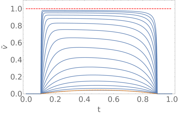
Figure 15: Entropy increase rates (88) for an interval from $x_{min}=0.1$ to $x_{max}=0.9$ as a function of time $t$. We have chosen a fixed $T_{R}=1$ and $T_{L}=1+10^{\alpha}$ with $\alpha=-1,-0.8,-0.6,...,2$, where $\alpha$ increases from the lowest solid curve in the figure to the highest one. The dotted (orange) line represents the curve expected from the universal low temperature formula (28) for $T_{R}=1,\ T_{L}=1.1$. The dashed (red) line signifies the bound (89).

A bound of the type (87) is especially interesting when compared to other velocities that are related to the spread of entanglement or other disturbances on the boundary of AdS_d+1, such as the entanglement velocity (67) and the butterfly effect velocity (68). As said before, the case $d=2$ is the special case where $1=v_{B}=v_{E}$, and hence the bound (87) can be expressed in terms of $v_{E}$ and/or $v_{B}$. As we will see in section 7.2, this may however not be the case for higher dimensions any more.

Nevertheless, we can attempt to interpret our findings for $2+1$ bulk dimensions in terms of the intuition provided by the study of the entanglement tsunami phenomenon. As noted in section 5.3 in discussing the result (82), in the limit where the entanglement entropy increases linearly ($\ell\gg T_{L}^{-1}$) with a rate saturating the bound (89), the shockwave seems to take the role that the entanglement tsunami had for a global quench. As the shockwave enters the interval only from one side instead of from both sides, the increase rate in (82) is only half of the one calculated in a global quench according to (66), where $A_{\Sigma}=2$ and $v_{E}=1$. As pointed out in section 5.1, the linear increase (66) is only valid when looking at large enough boundary regions (compared to the inverse of the temperature). Our analytical results (82) and especially (28) then show how this linear behaviour is modified when moving away from this limit: The linear increase of entropy characteristic of the entanglement tsunami is replaced by a much smoother S-shaped curve. This might, in analogy with the tsunami picture, be called an entanglement tide. It should be pointed out that in our matching procedure of section 4, the shockwave is always assumed to be infinitely thin, hence this modification is not a result of a finite shockwave size. Also, other works where the evolution of entanglement entropy away from the tsunami regime was studied are Kundu:2016cgh ; OBannon:2016exv ; Lokhande:2017jik , with somewhat contrasting results, as explained above.

6 Entanglement entropies of systems with many disconnected components

When working in $1+1$-dimensional CFTs, the subsystems for which entanglement entropy may be calculated are either isolated intervals or unions of $n$ intervals. It is known that for example in the case two intervals $A$ and $B$, there are two possible (physical, see section 6.1) configurations for calculating the entanglement entropy for the union of these two intervals, $S(AB)\equiv S(A\cup B)$, as shown in figure 16 Headrick:2007km ; Headrick:2010zt ; Allais:2011ys . By the HRT proposal Hubeny:2007xt , the entanglement entropy is given by the minimal possible configuration of extremal curves,

$$S(AB)=\min\left\{S(A)+S(B),S_{AB_{1}}+S_{AB_{2}}\right\}.$$ (91)

As the parameters defining $A$ and $B$ are varied, there may be phase transitions between these two configurations, and we will consequently refer to these configurations as phases. Interestingly, the entanglement entropies of the subsystem $A\cup B$ and its (sub)subsystems may be required to satisfy certain inequalities, which in the $n=2$ case discussed here are only the subadditivity (SA) Araki:1970ba

$$S(AB)\leq S(A)+S(B),$$ (92)

following immediately from the holographic prescription (91), and the triangle or Araki-Lieb inequality Araki:1970ba

$$S(AB)\geq|S(A)-S(B)|.$$ (93)

While this is well-known and straightforward for the $n=2$ case just discussed, some interest has recently emerged Ben-Ami:2014gsa ; Alishahiha:2014jxa ; Bao:2015bfa ; Mirabi:2016elb ; Bao:2016rbj for similar concepts for situations involving $n>2$ disconnected intervals. Here we present our study of this case, and apply it to the steady-state spacetime in subsection 6.4. The Wolfram Mathematica code that we use for this analysis is uploaded to the arXiv as an ancillary file together with this paper and with a sample of the numerical results that is obtained from the matching procedure of section 4. There is some overlap between the issues addressed in this section (especially subsection 6.1) and the ones investigated in Bao:2016rbj , which was published after most of this section was completed. Although we are working in a covariant (time-dependent) setting, the findings of Bao:2016rbj suggest that the code used in our ancillary file may still be optimized. However, it nevertheless produces the desired results.

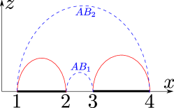
Figure 16: For the union of the two intervals $A$ (from 1 to 2) and $B$ (from 3 to 4), there are two possible ways how to calculate the entanglement entropy $S(A\cup B)$. One is by adding the entanglement entropies of the two intervals $A$ and $B$ (given by the solid red curves), the other is by adding the two curves $AB_{1}$ and $AB_{2}$, depicted as dashed blue curves.

6.1 The phases of the union of $n$ intervals

As shown in figure 16, for two intervals ($n=2$) there are two possible phases or configurations describing the entanglement entropy of the union of these intervals. Suppose we are given $n\in\mathbb{N}$ intervals, how many possible phases are there, and how do they look like? For a simplified situation where the lengths of all intervals are equal, as well as the distances between them, this has already been studied in Ben-Ami:2014gsa . We are however interested in the general case here. Of course, for any given $n$, the above question can simply be answered by drawing all possible configurations by hand. However, in this subsection we provide an algorithm that for any $n$ enumerates the possible phases in a consistent manner, without omitting any solution or counting it twice, and which can easily be implemented (see the corresponding ancillary file). We do not assume a translation invariant spacetime, however we will assume a spacetime with simple topology, such as Poincaré AdS or a flat black brane, excluding possible phenomena such as entanglement plateaux Hubeny:2013gta , see also Bao:2016rbj . Our task then essentially boils down to finding the noncrossing partitions of a set with $n$ elements, a well known combinatorial problem related to the Catalan numbers $C_{n}$ Catalan . We will, however, still present our solution to this problem in detail, as this exposition also serves to explain our notation and the inner workings of our ancillary file.

In a $1+1$ dimensional CFT, the $n$ intervals under consideration (which we assume to be all part of a specified equal time slice on the boundary) are all lined up one after the other, and we can enumerate their start- and end-points from $1$ to $2n$, as was already done in figure 16. Note that this is only an enumeration, and not meant to indicate the lengths of the different intervals or the coordinates of the boundary points for example.

Naively, in the $n=2$ case, we could have also drawn a configuration as the one depicted in figure 17, with two curves crossing each other Allais:2011ys . Such a configuration is, however, considered to be unphysical for various reasons. First, in the static case where the RT prescription holds, it can easily be shown that this type of configuration can never yield the lowest values for the entanglement entropy, hence can be ignored in (91) Headrick:2007km ; Allais:2011ys . Second, in a time dependent (HRT) case the two curves may not actually cross any more. However, the co-dimension one surface spanned between them and the boundary intervals would then become null or timelike at some point. As pointed out in Hubeny:2013gta , the co-dimension one surface required by the homology condition has to be restricted to be spacelike everywhere in the HRT prescription. Hence the configuration of figure 17 is also excluded in the dynamic case. Third, it has been discussed in Allais:2011ys that configurations of this intersecting type do not play a role when the (regularised) entanglement entropy of an interval is monotonously increasing with the interval length.

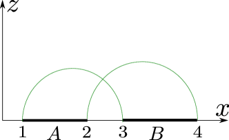
Figure 17: An unphysical configuration for $S(A\cup B)$.

When enumerating the possible phases of the entanglement entropy of the union of $n$ intervals, we therefore aim at excluding phases with curves intersecting when projected into the same plane, as shown in figure 17. Due to our labeling of the boundary points, it is clear that each interval begins at a point labeled by an odd number and ends at an even one. In figure 16, for $n=2$ we find one phase where bulk curves connect the points 1 to 2 and 3 to 4, and one phase where the bulk curves connect the points 1 to 4 and 2 to 3. In the unphysical case shown in figure 17 however, the points 1 to 3 and 2 to 4 are connected by bulk curves. We hence realize that in order to avoid intersections as the one shown in 17, each odd label has to be connected to an even label by a bulk curve. This means that each viable configuration for any $n$ has to be a mapping of the set of odd numbers $\{1,3,...,2n-1\}$ to the set of even numbers $\{2,4,...,2n\}$. The number of these possible mappings is given by $n!$, the number of possible permutations of the set $\{2,4,...,2n\}$,

$$\text{phase 1:\ }\left(\begin{array}[]{c}1\rightarrow 2\\ 3\rightarrow 4\\ 5\rightarrow 6\\ ...\\ 2n-1\rightarrow 2n\end{array}\right),\ ...,\ \text{phase i:\ }\left(\begin{array}[]{c}1\rightarrow\sigma_{i}(2)\\ 3\rightarrow\sigma_{i}(4)\\ 5\rightarrow\sigma_{i}(6)\\ ...\\ 2n-1\rightarrow\sigma_{i}(2n)\end{array}\right),...$$ (104)

Here, $\sigma_{i}$ is the $i$-th out of the $n!$ possible permutations of the set $\{2,4,...,2n\}$. Returning to the specific example of $n=2$, we hence obtain the two phases

$$S(AB)=S(A)+S(B)\ \Leftrightarrow\ \left(\begin{array}[]{c}1\rightarrow 2\\ 3\rightarrow 4\end{array}\right)\ \text{``disconnected phase'' ,}$$ (107)

$$S(AB)=S(AB_{1})+S(AB_{2})\ \Leftrightarrow\ \left(\begin{array}[]{c}1\rightarrow 4\\ 2\rightarrow 3\end{array}\right)\ \text{``connected phase'' ,}$$ (110)

where e.g. $1\rightarrow 2$ stands for the curve connecting the points 1 and 2.

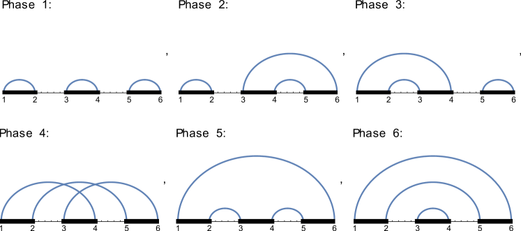
Figure 18: $3!=6$ preliminary configurations for $n=3$. Note that the 4th configuration is likely unphysical. According to the nomenclature of Ben-Ami:2014gsa , the phase 6 is referred to as engulfed phase.

All the possible phases obtained this way for $n=3$ are shown in figure 18. Clearly, there are $3!=6$ of them, however we see that there is still one involving intersections. Of course, when sketching these six possible configurations by hand, it is easy to identify the one involving intersections and to discard it. However, from our point of view of automatizing this process, we need to formulate and implement the criterion that distinguishes the unphysical phase

$$\left(\begin{array}[]{c}1\rightarrow 4\\ 3\rightarrow 6\\ 5\rightarrow 2\end{array}\right)$$ (114)

from the physical phases such as e.g.

$$\left(\begin{array}[]{c}1\rightarrow 4\\ 3\rightarrow 2\\ 5\rightarrow 6\end{array}\right).$$ (118)

To do so, we exclude all configurations in which there are two intervals spanned by the endpoints of bulk curves that intersect in such a way that the intersection is an interval that is not either empty or one of the intervals spanned by the bulk curves. For example, in the unphysical example (114) the curves span the intervals $[1,4]$, $[3,6]$ and $[2,5]$. The first and the last of these intersect in $[2,4]$ which is not one of the spanned intervals, hence this configuration is excluded as unphysical. In contrast, in the example (118) the curves span the set of intervals $\{[1,4],[2,3],[5,6]\}$, and apart from the empty interval the only intersection between these intervals is $[2,3]$, which is an element of the above set. Hence this phase is considered physical. See the ancillary file for a concrete implementation.

This approach allows us to implement a general algorithm that gives us all possible phases for the entanglement entropy of a set of $n$ disconnected intervals, with any $n$. For the case $n=3$, we then have to exclude phase 4 in figure 18, and are left with the five physical phases already identified in Allais:2011ys . For $n=4$ for example, the 14 physical phases are shown in figure 19. For general $n$, the number of these physical phases is given by the $n$-th Catalan number Catalan

$$C_{n}=\frac{1}{n+1}\left(\begin{array}[]{c}2n\\ n\end{array}\right),$$ (121)

which grows as $C_{n}\sim\frac{4^{n}}{n^{3/2}\sqrt{\pi}}$ for large $n$. However, with a more optimized code, it may not be necessary to compute all the values of this number of phases Bao:2016rbj .

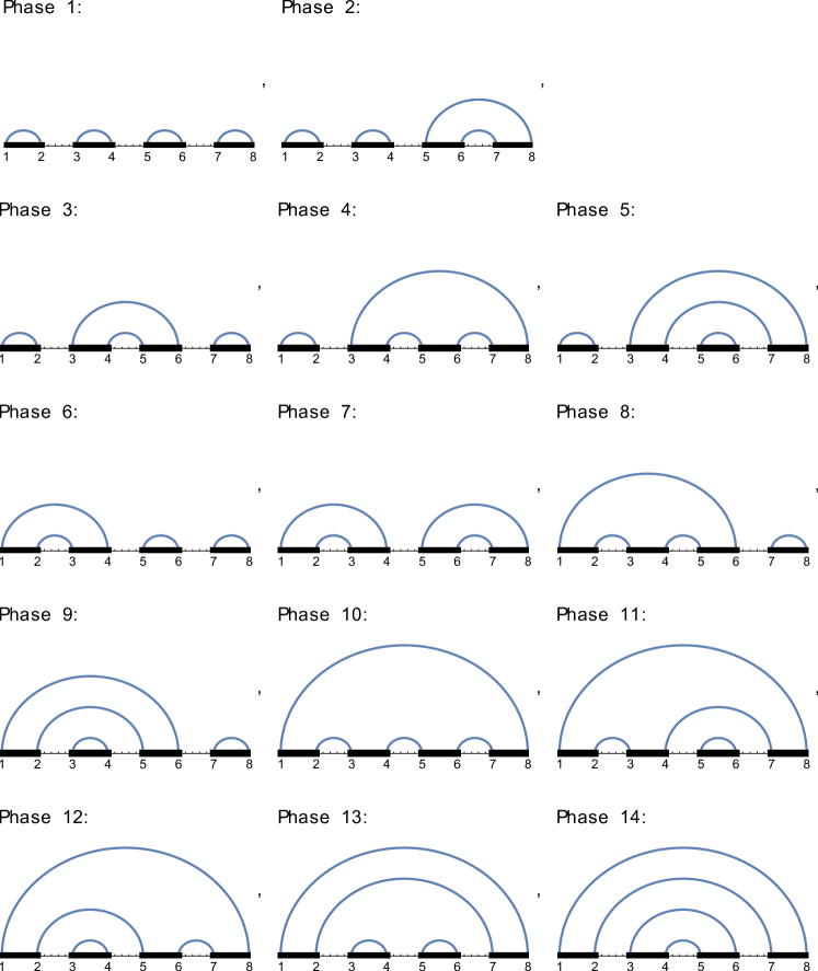
Figure 19: Physical configurations for $n=4$ intervals. Note that out of the $4!=24$ configurations that our counting would naively have suggested, there are only 14 physical ones, i.e. 14 ones where the curves do not intersect when projected to the same plane.

6.2 Inequalities for the union of $n$ intervals

Our interest in this section is to study the entanglement inequalities that can be formulated when working with $n>2$ intervals.

At the level $n=3$, the most well-known inequality that entanglement entropies are expected to satisfy is the strong subadditivity (SSA) doi:10.1063/1.1666274 , commonly stated as

$$S(AB)+S(BC)-S(ABC)-S(B)\geq 0.$$ (122)

A different inequality often associated with SSA is doi:10.1063/1.1666274

$$S(AB)+S(BC)-S(A)-S(C)\geq 0,$$ (123)

see Allais:2011ys ; Hayden:2011ag for a discussion of the relation between (122) and (123) in the holographic case. For the static holographic cases in which the Ryu-Takayanagi prescription Ryu:2006bv ; Ryu:2006ef applies, these two inequalities were proven in Headrick:2007km . For the case of time-dependent bulk spacetimes where the HRT prescription Hubeny:2007xt applies, a proof of (122) was given in Wall:2012uf using the null curvature condition, see also the review Prudenziati:2015cva .

Similarly at $n=3$, we encounter what is known as the monogamy of mutual information or alternatively negativity of tripartite information

$$I_{3}(A:B:C)\equiv S(A)+S(B)+S(C)-S(AB)-S(BC)-S(AC)+S(ABC)\leq 0.$$ (124)

This was proven for the static RT case in Hayden:2011ag , and for the time dependent HRT case in Wall:2012uf . There are many more possible inequalities that entanglement entropies for $n\geq 3$ intervals have to satisfy Linden2005 ; 6134666 , which can be seen to follow from (124) and the other inequalities discussed so far for $n\leq 3$ Hayden:2011ag . Hence these inequalities are also proven to hold in holography, assuming appropriate energy conditions.

The study of entanglement entropy inequalities in AdS/CFT is hence of very high importance for the understanding of holography. On the one hand, if it can be shown that holographic prescriptions satisfy certain entanglement inequalities that do not hold in general quantum theories, this would help distinguish quantum theories that can in principle have a simple holographic dual from those that cannot. On the other hand, if energy conditions in the bulk can be used to prove certain entanglement inequalities that have to hold in the dual, then conversely, it may be possible to derive novel bulk energy conditions from boundary entanglement entropies Lashkari:2014kda .

In the following, we will hence use the entanglement entropies that we have calculated in our time dependent background metric (10) using the matching procedure of section 4 to test, for the manifestly time dependent HRT case, the validity of some of the entanglement inequalities derived in Bao:2015bfa for the static RT case. It should however be noted that as the metric (10) is a vacuum solution to Einstein’s equations everywhere, it trivially satisfies all common energy conditions, and is hence considered to be a physical spacetime. We hence do not expect any of the inequalities of Bao:2015bfa to be violated, however as their proof is only valid in the static case, it is interesting to test this expectation thoroughly. At the level of $n=5$ boundary intervals, these inequalities read

$$S(ABC)+S(BCD)+S(CDE)+S(DEA)+S(EAB)-S(ABCDE)$$

$$-S(BC)-S(CD)-S(DE)-S(EA)-S(AB)\geq 0$$ (125)

$$2S(ABC)+S(ABD)+S(ABE)+S(ACD)+S(ADE)+S(BCE)+S(BDE)$$

$$-S(AB)-S(ABCD)-S(ABCE)-S(ABDE)-S(AC)-S(AD)-S(BC)$$

$$-S(BE)-S(DE)\geq 0$$ (126)

$$S(ABE)+S(ABC)+S(ABD)+S(ACD)+S(ACE)+S(ADE)+S(BCE)$$

$$+S(BDE)+S(CDE)-S(AB)-S(ABCE)-S(ABDE)-S(AC)$$

$$-S(ACDE)-S(AD)-S(BCD)-S(BE)-S(CE)-S(DE)\geq 0$$ (127)

$$S(ABC)+S(ABD)+S(ABE)+S(ACD)+S(ACE)+S(BC)+S(DE)$$

$$-S(AB)-S(ABCD)-S(ABCE)-S(AC)-S(ADE)-S(B)-S(C)$$

$$-S(D)-S(E)\geq 0$$ (128)

$$3S(ABC)+3S(ABD)+3S(ACE)+S(ABE)+S(ACD)+S(ADE)+S(BCD)$$

$$+S(BCE)+S(BDE)+S(CDE)-2S(AB)-2S(ABCD)-2S(ABCE)$$

$$-2S(AC)-2S(BD)-2S(CE)-S(ABDE)-S(ACDE)-S(AD)-S(AE)$$

$$-S(BC)-S(DE)\geq 0$$ (129)

A further quantity of interest is the $n$-partite information,

$$I_{n}(A_{1}:A_{2}:A_{3}:...:A_{n})\equiv\sum_{i=1}^{n}S(A_{i})-\sum_{i<j}^{n}S(A_{i}\cup A_{j})+\sum_{i<j<k}^{n}S(A_{i}\cup A_{j}\cup A_{k})$$

$$\mp...-(-1)^{n}S(A_{1}\cup A_{2}\cup...\cup A_{n}),$$ (130)

generalising the concept of three-partite information introduced in (124). In a holographic context, quantities such as four- and five-partite information where studied for example in Alishahiha:2014jxa ; Mirabi:2016elb . In fact, based on the examples studied in those papers, the authors proposed the entanglement inequalities

$$I_{4}(A:B:C:D)\geq 0$$ (131)

and

$$I_{5}(A:B:C:D:E)\leq 0.$$ (132)

While the inequalities (131) and (132) may be true for the special cases studied in Alishahiha:2014jxa ; Mirabi:2016elb , where all intervals have the same length and distance from their neighboring intervals, it was already stated in Hayden:2011ag that (131) and (132) do not hold in general holographic setups. In fact, using the numerical data for the time dependent backgrounds studied in this paper or simply data valid for static backgrounds such as the BTZ metric (3) and feeding this data into our ancillary file, it is possible to find explicit examples for sets of four or five intervals that will lead to violations of the proposed inequalities (131) and (132).

6.3 Symmetries of entanglement inequalities

In section 6.1 we have described how we can systematically enumerate all the possible phases that the entanglement entropy of the union of $n$ intervals can have. In order to check the validity of inequalities for entanglement entropy using this counting procedure, it is also important to consider the symmetries of the inequalities under consideration. Take as the simplest example the strong subadditivity inequality (122), valid for the combination of the $n=3$ intervals $A,B,C$. Comparing to our enumeration introduced in section 6.1, see also figure 18, it is clear that a priori there may be five different physical configurations determining the quantity $S(ABC)$. However, there are different ways to assign the labels $A,B,C$ to the intervals $[1,2],[3,4],[5,6]$ in figure 18. If we impose a strict alphabetical ordering $A=[1,2],B=[3,4],C=[5,6]$, the inequality (122) will not be equivalent for example to the inequality

$$S(AB)+S(AC)-S(ABC)-S(A)\geq 0,$$ (133)

which we obtained by relabeling $A$ and $B$. On the other hand, (122) is invariant under interchanging $A$ and $C$. This means that entanglement inequalities involving many intervals may have a non-trivial amount of symmetry (or asymmetry) under permutation (or renaming) of intervals $A,B,C,...$ which we will have to take into account when employing a strict enumeration of intervals from left to right as we do in section 6.1 and in our numerical code for technical reasons.

In our ancillary file, we solve this problem as follows: Take an inequality, e.g. (122), in a form where the intervals are denoted $A,B,C,...$ without assuming a specific ordering of them on the boundary. We then write the inequality with all elements to the left of an $\geq$ sign, and represent it as a set of sets of elements, e.g.

$$\{\{A,B\},\{B,C\},\{-B\},\{-A,-B,-C\}\}.$$ (134)

It is then easy to apply all possible permutations to this set, and filter out the ones that act non-trivially, i.e. that do not leave it invariant. In the end, we are left with a list of sets of the form (134), which correspond to inequalities which are inequivalent when using a strict alphabetical ordering $A=[1,2],B=[3,4],...$ of the intervals along the boundary. In this context, it is interesting to note that the degree of symmetries uncovered this way varies from one inequality to the other. For example, while by permuting the intervals $A,B,C,D,E$ (which in this subsection are now assumed to be ordered alphabetically on the boundary) gives us 10 inequivalent inequalities following from (127), this number is 60 for (129).

6.4 Analysis and Results

We now have almost all prerequisites that are needed in order to check the validity of entanglement inequalities such as (125) - (129) in the time dependent system holographically described by the bulk metric (10). As the matching-procedure outlined in section 4 can only be applied when the geodesics cross the shockwave once, we have to restrict ourselves to the study of intervals for which all boundary points have $x$-coordinates either larger than zero or smaller than zero. We generally assume all boundary points of intervals under investigation to be located at equal boundary time.

We have carried out this analysis for various choices of temperatures $T_{L}$ and $T_{R}$, for various values of the boundary time $t$, and for intervals to the left and to the right of $x=0$. As the results were qualitatively similar in all these cases, we will in the following only discuss the example where we chose $T_{L}=9,T_{R}=1$ (hence $\beta=\frac{4}{5}$) and the boundary time slice to be at $t=1$, with intervals in the range $x>0$. According to our discussion in section 6.1 there will be $42$ possible phases that the entanglement entropy of $n=5$ intervals can take. Furthermore, in a non-homogeneous system, $n$ intervals are defined by $2n$ boundary points. As our calculations will be numerical, we are faced with a severe problem: Even if we are able to check the validity of inequalities such as (125) - (129) for any given set of five intervals, how can we make sure that we find all potentially interesting cases? After all, we have to cover a $2n$ dimensional parameter space, on which phase transitions between $42$ different phases can occur. Numerically, we will of course only be able to check a finite number of examples. Naively, the best idea appears to be to take a finite number of evenly spaced points on the boundary,

$$x=0.1,0.2,0.3,...,2.0$$ (135)

and to calculate the entanglement entropy for any interval formed by any two of these points. From this data, we may then calculate the entanglement entropy of the union of any possible set of $n$ intervals that can be formed from the given boundary points, and subsequently check the validity of all entanglement inequalities of interest.

However, we can do better than this. In the study of mutual information for Poincaré backgrounds, where there are only two phases as shown in figure 16, it is known that the phase will depend on the relation between the sizes of the two intervals and the distances between them. In our attempt to cover the relevant phase space for $n\leq 5$ intervals, it will hence be advantageous to allow for the distances between boundary points to vary between as many orders of magnitude as possible. Instead of using equally spaced boundary points such as in (135), the idea is thus to use points which are positioned in a fractal-like way, e.g.

$$x=0,1-\frac{2}{\alpha},1-\frac{4}{\alpha^{2}},1-\frac{8}{\alpha^{3}},...,1+\frac{8}{\alpha^{3}},1+\frac{4}{\alpha^{2}},1+\frac{2}{\alpha},2,$$ (136)

where we have found that the choice $\alpha=9/2$ gives a good trade-off between the orders of magnitude of length scales covered and the overall number $N$ of points, which for a reasonable runtime of our numerics we would like to keep at $N=20$.

Using the matching prescription explained in section 4, we have calculated the renormalised lengths of the geodesics connecting any two of the $N=20$ boundary points under consideration. In our case at hand, this requires $\frac{1}{2}N(N-1)=190$ calculations. As a next step, for some $n\leq 5$ we want to form $n$ boundary intervals by selecting $2n$ boundary points out of the $N$ available points. Obviously, there are

$$\left(\begin{array}[]{c}N\\ 2n\\ \end{array}\right)=\frac{N!}{(2n)!(N-2n)!}$$ (139)

ways to do so. Given our $N=20$ points positioned on the boundary time slice $t=1$ according to the sequence (136), we are hence for example able to study $184756$ distinct unions of $n=5$ non-adjacent boundary intervals. For all these $184756$ different cases, it is then possible to calculate the entanglement entropy, see figure 20. Interestingly, in the case at hand we find that out of the $184756$ available unions of intervals, $100177$ are in the totally disconnected phase in which $S(A_{1}\cup A_{2}\cup...)=S(A_{1})+S(A_{2})+...$, and in which hence the entanglement inequalities (124)-(132) are trivially saturated. Consequently, only the remaining $84579$ cases will be of further interest. It should also be noted that the overall value of the entanglement entropy for a given union of intervals is dependent on the explicit cutoff used in our numerics. However, the linear combinations of entanglement entropies appearing in the inequalities (122), (124) but also (125)-(129), are always balanced in such a way that the cut-off dependence of the individual terms cancels, such that the result is physical.

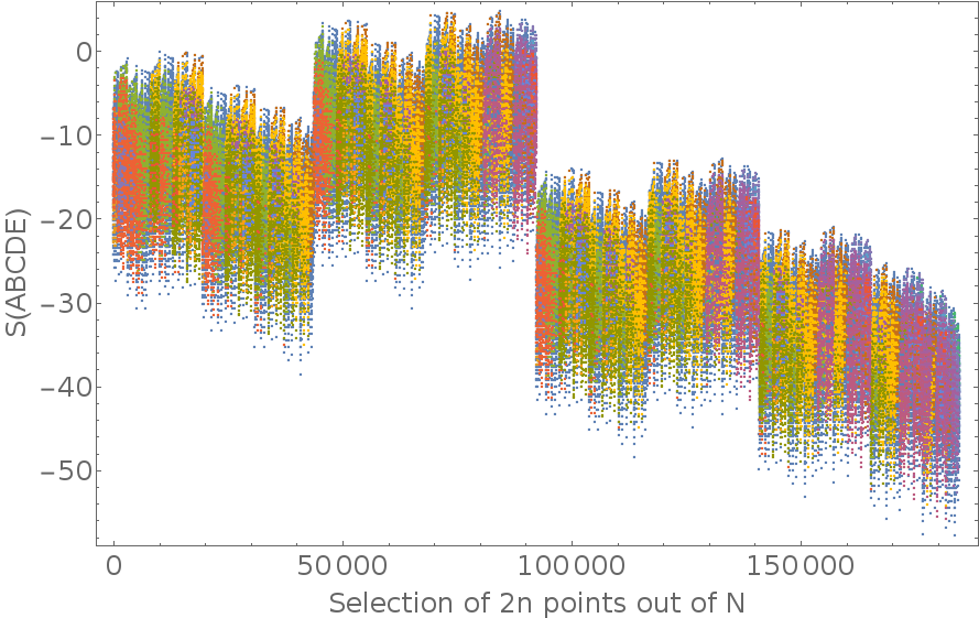
Figure 20: Entanglement entropies for all $184756$ possible unions of $n=5$ non-adjacent intervals formed out of the $N=20$ boundary points (136) at $t=1$, for $T_{L}=9$ and $T_{R}=1$. The value of the entanglement entropy is dependent on the explicit cut-off or renormalisation scheme used, so the overall shift of the vertical axis is of no relevance, only linear combinations of entanglement entropies in which the cut-off dependence cancels are physical. The colour represents the different phases that the entanglement entropy of the union of five intervals can be in. The intricate structure of the data over the horizontal axis is due to the lexicographic order in which the $184756$ possible unions of $n=5$ intervals are enumerated and the placement of the boundary points according to (136).

Now, we have all the necessary ingredients together to check the validity of various entanglement inequalities, as well as of their permutated versions as discussed in section 6.3. The results are as follows:

• At $n=3$, both strong subadditivity (122) and monogamy of mutual information (124) are satisfied, as expected based on Wall:2012uf ; Prudenziati:2015cva . In contrast to Ben-Ami:2014gsa , we find that even the engulfed phase (see figure 18) can be the minimal one in specific examples. Generically, this seems to happen when the middle interval is very small compared to the gap between the other two intervals.

• At $n=4$, the only inequality that we are checking is the positivity of four-partite information (131). In fact, in contrast to Alishahiha:2014jxa ; Mirabi:2016elb , we find a number of examples for sets of four intervals where this inequality is violated. However, as it was pointed out in Hayden:2011ag and was explicitly checked by us, this is not a particular feature of the time dependent case, and happens already in holographic systems with static bulk-spacetime duals.

• At $n=5$, we find numerous violations of the negativity of five-partite information (132), see the similar discussion for $n=4$. In fact, out of the $184756$ total and $84579$ nontrivial sets of five intervals under investigation, we find a violation of (132) in $417$ cases. It is also noteworthy that even for the $84579$ cases where five-partite information does no have to vanish a priori, the result that we obtain vanishes within numerical accuracy for $81183$ cases, see figure 21.

  Furthermore, we check the inequalities (125)-(129) as well as all their relevant permutations, see section 6.3. The result is that we find not a single case in which any of these inequalities is violated, neither for the specific example currently at hand ($T_{L}=9,T_{R}=1,t=1$) nor for any other example that we studied. See for example figure 22. We view this as a clear indication that the inequalities (125)-(129), although so far only proven in the static case, will generally also hold in physical time-dependent cases.

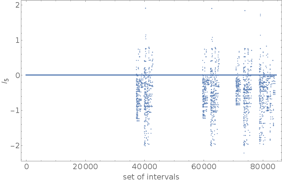
Figure 21: Five-partite information for the $84579$ sets of five intervals (out of initially $184756$) for which the total entanglement entropy is not in the totally disconnected phase. Clearly there are multiple violations of the proposed inequality (132). As in figure 20, we are here displaying results for the example where $T_{L}=9$, $T_{R}=1$ and the boundary time $t=1$.

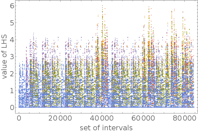
Figure 22: The left-hand sides of the inequality (125) for the $84579$ sets of five intervals (out of initially $184756$) for which the total entanglement entropy is not in the totally disconnected phase. Clearly there are no violations of the inequality (125). The different colors in the figure stand for different permutations, as explained in section 6.3. As in figure 20, we are here displaying results for the example where $T_{L}=9$, $T_{R}=1$ and the boundary time $t=1$.

7 Comments on higher dimensions

7.1 State of the art in $d>2$

After investigating the one-dimensional case in detail, it is natural to ask about a generalisation to higher dimensions. That case is, however, much subtler. It has already been addressed in various works. Let us briefly summarize the current state of discussion about the higher-dimensional case. In Bhaseen:nature , a straightforward generalization of the 1+1 dimensional model was suggested, namely a solution consisting of two shockwaves, not necessarily travelling with identical velocities, and a non-equilibrium steady state between the shocks. Such a solution was numerically found in the hydrodynamic regime Bhaseen:nature . Later, a similar solution beyond the hydrodynamic approximation was found in Amado:2015uza , in the framework of gauge/gravity duality. However, at the hydrodynamical level an inconsistency between the non-equilibrium steady-state (NESS) conjecture of Bhaseen:nature and thermodynamics was pointed out in Spillane:2015daa . The issue is as follows: The setup of two heat baths put in contact at an initial time is essentially a classical Riemann problem of solving partial differential equations. For this type of problem, there is a so-called entropy condition. This is a requirement that characteristic lines of the differential operator involved, i.e. curves along which the initial condition is transported, always end rather than begin on the shock wave. The name ‘entropic condition’ comes from the fact that if characteristics end at some point, the information about the initial state is lost and hence the entropy is produced. If the characteristics started at the discontinuity, the system would require fixing an initial condition on the shockwave, such that information would be produced and entropy would decrease. A detailed analysis of this condition for higher dimensions leads to the conclusion that while a shockwave moving from the region of higher temperature to the colder one is a entropically valid solution, a shock moving in the opposite direction is not (see section 3 of Spillane:2015daa for details). The results of Spillane:2015daa imply that the solution involving two shockwaves is valid in $d=2$ only, when the velocities of the shocks are identical and equal to one. In higher dimensions, to stay in agreement with entropic considerations, we have to replace the unphysical shockwave by a new solution – the rarefaction wave – which is continuous but not smooth and much wider than the shockwave. Let us stress that the double-shock solution is not mathematically incorrect since for complicated non-linear PDEs, uniqueness of solutions is not always guaranteed for arbitrary types of boundary or initial conditions. The double shockwave is however non-physical due to the entropic reasons mentioned. The physical solution is unique in the sense that the shock-rarefaction solution is realised in nature. Let us however emphasize that as shown in Spillane:2015daa , the double-shock solution is a valid, physically correct and unique solution to the initial value problem of our non-linear equation in $d=2$.

An important question about the shock-rarefaction solution in higher dimensions is whether it does support the existence of a NESS, defined as a region with constant energy current that can be obtained by boosting a static thermal state with some effective temperature. There are two possibilities: Either the rarefaction solution extends over a large enough region and reaches the existing shock, excluding the formation of NESS, or the rarefaction wave is relatively compact and a NESS is formed between the rarefaction and the shock wave on the other side. In Lucas:2015hnv , the authors argue in favour of the latter, based on numerical studies for hydrodynamical setups. Moreover they discover that for most conditions, the quantitative difference of observables obtained in a non-physical dual-shock solution and those obtained in the thermodynamically favoured rarefaction-shock solution is of order of a few percent. The specific properties of the steady state remain similar to the universal behaviour of the NESS in Bhaseen:nature .
A further question is whether the dual gravity description allows for a physical rarefaction-shock solution. An example of such a solution was found in Herzog:2016hob in the limit of large dimensions $d\rightarrow\infty$. However, obtaining a clear, numerical shock-rarefaction solution in the gauge/gravity framework in $d=3$ or $4$ dimensions and testing its properties such as stability is still an open problem. It is worth noting that the authors of Amado:2015uza found a full numerical solution of an ‘almost’ Riemann problem where the initial condition is a smooth approximation of a step function, as our (13) in the framework of AdS/CFT. Since, as discussed previously, the values of the observables obtained from the shock-rarefaction solution and the double shock solution differ only by a few percent, it is not clear which of them is the holographic dual of the hydrodynamic solution. The authors of the previously mentioned paper themselves state that their solution seems to agree with the double-shock conjecture, the work however was published before the entropic issues of the double shock solutions were pointed out in Spillane:2015daa .

The arguments mentioned here ensure that a qualitative analysis of the entanglement entropy in higher dimensions can be carried out, based on the simple NESS model of Bhaseen:nature . We devote this section to this analysis.

7.2 Analytical considerations

Here we present analytical results for the higher-dimensional cases. These are obtained by assuming that the dual-shock solution is valid at least approximately. While the higher dimensional analogue of the time-dependent metric (10) is not known analytically any more, we still know the boosted black-brane line element generalising (6) to higher dimensions Bhaseen:nature

$$ds^{2} =\frac{L^{2}}{z^{2}}\left(\frac{dz^{2}}{f(z)}-f(z)\left(\cosh\theta dt-\sinh\theta dx\right)^{2}+\left(\cosh\theta dx-\sinh\theta dt\right)^{2}+dy_{\perp}^{2}\right),$$

$$f(z) =1-\left(\frac{z}{z_{H}}\right)^{d},\ z_{H}=\frac{d}{4\pi T}.$$ (140)

Setting $\theta=0$ and $T=T_{L}$ or $T=T_{R}$, we recover the metrics of the initial static black branes. For the late time steady state, the boost parameter (or rapidity) $\theta$ is given by Bhaseen:nature

$$T =\sqrt{T_{L}T_{R}},$$ (141)

$$\chi =\left(\frac{T_{L}}{T_{R}}\right)^{\frac{d}{2}},$$ (142)

$$\beta =\frac{\chi-1}{\sqrt{\left(\frac{1}{d-1}+\chi\right)(d-1+\chi)}},$$ (143)

$$\theta =\text{arctanh}\beta,$$ (144)

where $\beta$ is the boost velocity. It is also important to note that in higher dimensions, the two shockwaves move with different velocities, Bhaseen:nature

$$u_{L}=\frac{1}{d-1}\sqrt{\frac{\chi+d-1}{\chi+\frac{1}{d-1}}},\ \ u_{R}=\sqrt{\frac{\chi+\frac{1}{d-1}}{\chi+d-1}}.$$ (145)

Interchanging $T_{L}$ and $T_{R}$ means $\chi\rightarrow 1/\chi$ and under this transformation $u_{L}\leftrightarrow u_{R}$.

Although the entanglement entropy $S(\ell)$ for a strip of width $\ell$ and infinite extent in the $dy_{\perp}$ directions cannot be calculated analytically in the background (140), we find that in the limit $\ell\rightarrow\infty$ where the entanglement entropy becomes extensive, the entropy density analytically reads

$$s_{eq} =\frac{1}{4G}\left(\frac{4\pi TL}{d}\right)^{d-1}\cosh\theta.$$ (146)

$$=\frac{(4\pi L)^{d-1}}{4Gd^{d}}\sqrt{\left(\left(\frac{T_{L}}{T_{R}}\right)^{\frac{d}{2}}+d-1\right)\left((d-1)\left(\frac{T_{L}}{T_{R}}\right)^{\frac{d}{2}}+1\right)}\left(\frac{T_{R}}{T_{L}}\right)^{\frac{d}{4}}(T_{L}T_{R})^{\frac{d-1}{2}}$$ (147)

Let us consider the question whether meaningful statements, similar to (84), about the (average) entropy increase rates of a strip in this setup may also be found for higher dimensions. Due to the form of the velocities (145), we see that the time the shockwave takes to pass through a strip of width $\ell$ is

$$\Delta t_{L/R}=\frac{\ell}{u_{L/R}}.$$ (148)

Just as in section 5.4, we may calculate the average increase/decrease rate of entanglement entropy. We assume for now that the entanglement is only influenced by the shockwaves, and not the light cones. We find

$$v_{av,\,L/R}=\frac{\Delta S_{L/R}}{\Delta t_{L/R}}\rightarrow\frac{1}{4G}\left(\frac{4\pi L}{d}\right)^{d-1}u_{L/R}\left(T^{d-1}\cosh\theta-T_{L/R}^{d-1}\right)$$ (149)

for $\ell\rightarrow\infty$. Consequently, in analogy to (86),

$$\tilde{v}_{av,\,L} =\frac{v_{av,\,L}}{s_{eq}}=u_{L}\left(1-\frac{\chi^{\frac{d-1}{d}}}{\cosh\theta}\right)=\frac{\sqrt{(d-1+\chi)((d-1)\chi+1)}-d\chi^{\frac{d-1}{d}+\frac{1}{2}}}{\sqrt{d-1}((d-1)\chi+1)},$$ (150)

$$\tilde{v}_{av,\,R} =\frac{v_{av,\,R}}{s_{eq}}=u_{R}\left(1-\frac{\chi^{\frac{1-d}{d}}}{\cosh\theta}\right)=\sqrt{\frac{\frac{1}{d-1}+\chi}{d-1+\chi}}\left(1-\frac{d\chi^{\frac{1}{d}}}{\sqrt{\chi(d-1+\chi)((d-1)\chi+1)}}\right).$$ (151)

As a consistency check, we see that under $T_{L}\leftrightarrow T_{R}$, $\tilde{v}_{av,\,L}\leftrightarrow\tilde{v}_{av,\,R}$. Also, for $d=2$ this exactly reproduces our findings from section 5.4. Interestingly, in contrast to (87), we find that while these formulas imply an upper bound

$$\tilde{v}_{av,\,L,R}(\chi)\leq 1$$ (152)

on the normalised average entropy increase, we do not find a lower bound on $\tilde{v}_{av,\,L,R}$ limiting the entropy decrease for $d>2$. In figure 23, the two functions $\tilde{v}_{L/R}(\chi)$ are plotted for $d=2,3,4$. We see that in higher dimensions, due to (152), $\tilde{v}_{av}$ may exceed both $v_{E}$ and $v_{B}$ defined in section 5.4. However, only a full numerical solution of the higher dimensional case will produce a clearer picture of the relation between the entropy increase rate for a given intervals and other bounds or quantities such as (67) or (68). Such a numerical solution will also allow to address the impact of considering a shock or a rarefaction wave in relation to the absence of a lower bound on $\tilde{v}_{av}$ in $d>2$. This may be relevant for a general discussion of whether choosing a gravity solution that decreases the thermodynamic entropy has unphysical consequences for the entanglement entropy.

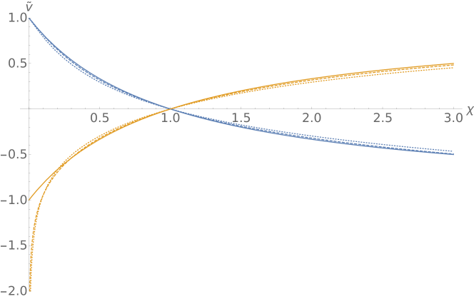
Figure 23: Normalised entropy increase and decrease rates (150),(151) for $d=2$ (solid), $d=3$ (dashed) and $d=4$ (dotted) as a function of $\chi$. Note that in the formulas (150),(151), $\tilde{v}_{L}>0$, $\tilde{v}_{R}<0$ for $\chi>1$ and $\tilde{v}_{L}<0$, $\tilde{v}_{R}>0$ for $\chi<1$. While $1\geq\tilde{v}_{L,R}\geq-1$ for $d=2$, we see that $1\geq\tilde{v}_{L,R}$ with no lower bound for $d>2$.

7.3 Numerical considerations

Refs. Megias:2015tva ; Megias:2016vae give a solution of the background equations of motion on the gravity side in the case $d\geq 2$ by considering a linearization of the system. This approach turns out to be equivalent to linearized hydrodynamics, as it is valid as long as $|T_{L}-T_{R}|<|T_{L}+T_{R}|$. Using this background, we may compute numerically the entanglement entropy for any number of dimensions by following the procedure of Sec. 3. The result for $d=3$ and moderate values of $\ell$ is shown in Figs. 24 and 25.  These figures display that in contrast to the case $d=2$ studied in Sec. 3, the ‘conservation’ of entanglement entropies between $t=0$ and $t=\infty$ given by (36) turns out to be not valid for $d=3$, at least within the linearization procedure chosen.  As a consequence, the possible existence of a universal behavior for the time evolution of entanglement entropies analogous to (28) is not obvious in this case. However, the increase of the mutual information with time $\partial_{t}I(A,B)\geq 0$, cf. Eq. (31), appears to be a robust property valid also for $d=3$, and the same can be said for the decrease of $S(A\,\cup B)$ with time. A more detailed study of these issues will be addressed elsewhere.

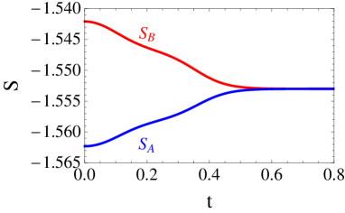
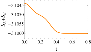
Figure 24: (Left) Renormalized entanglement entropies $S_{A}$ and $S_{B}$ as a function of time, in a system with $d=3$. (Right) Renormalized entanglement entropy $S_{A}+S_{B}$ as a function of time. In both figures we have considered the linearized background computed in Refs. Megias:2015tva ; Megias:2016vae , the intervals $x^{A}\in[0.05,0.275]$ and $x^{B}\in[-0.275,-0.05]$, and temperatures $T_{L}=0.6$ and $T_{R}=0.5$. We have set $G=1$ and $L=1$.

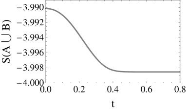
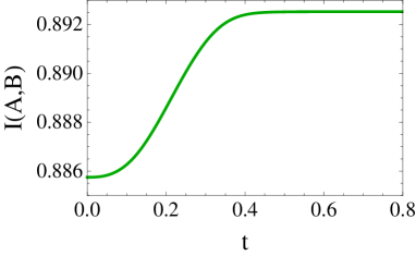
Figure 25: (Left) Renormalized entanglement entropy of $A\,\cup B$ as a function of time. (Right) Mutual information of $A$ and $B$ as a function of time. We consider a system with $d=3$ within the linearized background of Refs. Megias:2015tva ; Megias:2016vae , with the same configuration as in Fig. 24.

8 Conclusion and outlook

In this work we have studied a holographic model for far-from-equilibrium dynamics that describes the time-dependent properties of energy flow and information flow of two thermal reservoirs initially isolated. In this system, a universal steady state develops, described by a boosted black brane. A relevant observable that provides physical insight into the evolution of the system is the entanglement entropy, which measures the information flow between two subsystems. By using the exact solution for $d=2$ provided in Bhaseen:nature , we have studied the time evolution of the entanglement entropy, and characterized some universal properties of the quenching process. We also studied the time evolution of mutual information and found it to monotonically grow in time.

In section 5, after a brief overview of velocity bounds for entropy spread and increase, we have investigated the matching procedure outlined in section 4 in more detail, showing that in certain circumstances an analytical solution is possible. This allowed us to prove the validity of the universal formula (28) in the appropriate low temperature limits. In subsection 5.4, we then investigated the increase rates of entanglement entropy obtained using the numerical and analytical results of the previous sections. We find that both averaged and momentary entanglement entropy increase and decrease rates are bounded by the speed of light (89). While this bound is close to being saturated for intervals that are large compared to the scale set by the temperature, this is not the case for smaller intervals, where the universal formula (28) becomes a good approximation, see again figure 15. This indicates that the shockwave in our setup, which in many ways is similar to a local quench, mimics an entanglement tsunami for large interval sizes $\ell$, leading to a linear entropy increase with the appropriate rate. For small $\ell$ however, the universal behaviour (28) with its characteristic S-shape takes over. We refer to this as an ‘entanglement tide’. As discussed in section 7, it will be very interesting to study these questions for analogous systems in higher dimensions, where the speed of light, the entanglement velocity $v_{E}$ and the butterfly velocity $v_{B}$ are not equivalent any more. This may help to get a better understanding of the mechanisms related to entanglement tsunamis.

Apart from the monogamy of mutual information and strong subadditivity, other inequalities involving a large number of subsystems have been proven in the static case, see Bao:2015bfa . In section 6, we have studied various entanglement entropy inequalities, which were proposed for up to $n=5$ intervals, in the present time-dependent system. What we found was that the inequalities proven in Bao:2015bfa also hold in the time-dependent system under consideration in this paper, at least in all cases that we numerically checked. However, we found that the signs of four- and five-partite information are not definite in this holographic system, in contrast to the results of Alishahiha:2014jxa ; Mirabi:2016elb . As the bulk metric investigated in this paper is a vacuum solution everywhere, and hence trivially satisfies the most common energy conditions, we did not have any a priori reason to expect encountering a violation of the entanglement entropy inequalities of Bao:2015bfa . It may hence be an interesting possibility for future research to check the validity of these inequalities for time-dependent bulk spacetimes that violate, for example, the null energy condition (NEC), similarly to what was done for strong subadditivity in Prudenziati:2015cva ; Allais:2011ys ; Callan:2012ip ; Caceres:2013dma . With this paper, we also upload the numerical code used to obtain the results of section 6 to the arXiv. We hope that this will facilitate future research in this direction.

One of the possible further directions of investigation is suggested by the elegant analytical behaviour of the entanglement entropy in the small temperature limit. It is known that low-energy behaviour of ballistic, quantum-mechanical models is well described by conformal field theories. For a thermal state this means that in the low-temperature regime of lattice model may be approximated by a thermal state of a CFT since that is a situation in which lower part of energy spectrum determines properties of the theory, as more excited states are not occupied. Therefore, we presume that the simple universal evolution of the entanglement entropy we observe should be as well visible in lattice (i.e. tensor network or exact diagonalisation) calculations. It will be interesting to compare to that kind of models, as local quenches in such systems have recently drawn some attention, see for example Bohrdt:2016vhv . Moreover, it is conceivable that further physically observables can be computed in that low-temperature limit.

Finally, comparisons to non-equilibrium hydrodynamics may provide further useful information. Recent work on this includes Romatschke:2017vte . Universal structures in a holographic model of non-equilibrium steady states, which are spatial analogues of quasinormal modes, have recently been considered in Sonner:2017jcf .

References

- (1) U. H. Danielsson, E. Keski-Vakkuri and M. Kruczenski, Black hole formation in AdS and thermalization on the boundary, JHEP 02 (2000) 039, [hep-th/9912209].
- (2) D. Grumiller and P. Romatschke, On the collision of two shock waves in AdS(5), JHEP 08 (2008) 027, [0803.3226].
- (3) S. Bhattacharyya, V. E. Hubeny, R. Loganayagam, G. Mandal, S. Minwalla, T. Morita et al., Local Fluid Dynamical Entropy from Gravity, JHEP 06 (2008) 055, [0803.2526].
- (4) P. M. Chesler and L. G. Yaffe, Horizon formation and far-from-equilibrium isotropization in supersymmetric Yang-Mills plasma, Phys. Rev. Lett. 102 (2009) 211601, [0812.2053].
- (5) E. Berti, V. Cardoso, L. C. B. Crispino, L. Gualtieri, C. Herdeiro and U. Sperhake, Numerical Relativity and High Energy Physics: Recent Developments, Int. J. Mod. Phys. D25 (2016) 1641022, [1603.06146].
- (6) M. Guo, C. Niu, Y. Tian and H. Zhang, Applied AdS/CFT with Numerics, PoS Modave2015 (2016) 003, [1601.00257].
- (7) V. Cardoso et al., NR/HEP: roadmap for the future, Class. Quant. Grav. 29 (2012) 244001, [1201.5118].
- (8) J. Abajo-Arrastia, J. Aparicio and E. Lopez, Holographic Evolution of Entanglement Entropy, JHEP 11 (2010) 149, [1006.4090].
- (9) V. Balasubramanian, A. Bernamonti, J. de Boer, N. Copland, B. Craps, E. Keski-Vakkuri et al., Thermalization of Strongly Coupled Field Theories, Phys. Rev. Lett. 106 (2011) 191601, [1012.4753].
- (10) V. Balasubramanian, A. Bernamonti, J. de Boer, N. Copland, B. Craps, E. Keski-Vakkuri et al., Holographic Thermalization, Phys. Rev. D84 (2011) 026010, [1103.2683].
- (11) V. Balasubramanian, A. Bernamonti, N. Copland, B. Craps and F. Galli, Thermalization of mutual and tripartite information in strongly coupled two dimensional conformal field theories, Phys. Rev. D84 (2011) 105017, [1110.0488].
- (12) H. Liu and S. J. Suh, Entanglement Tsunami: Universal Scaling in Holographic Thermalization, Phys. Rev. Lett. 112 (2014) 011601, [1305.7244].
- (13) Y.-Z. Li, S.-F. Wu, Y.-Q. Wang and G.-H. Yang, Linear growth of entanglement entropy in holographic thermalization captured by horizon interiors and mutual information, JHEP 09 (2013) 057, [1306.0210].
- (14) H. Liu and S. J. Suh, Entanglement growth during thermalization in holographic systems, Phys. Rev. D89 (2014) 066012, [1311.1200].
- (15) M. Alishahiha, A. Faraji Astaneh and M. R. Mohammadi Mozaffar, Thermalization in backgrounds with hyperscaling violating factor, Phys. Rev. D90 (2014) 046004, [1401.2807].
- (16) S. Kundu and J. F. Pedraza, Spread of entanglement for small subsystems in holographic CFTs, Phys. Rev. D95 (2017) 086008, [1602.05934].
- (17) P. Caputa, M. Nozaki and T. Takayanagi, Entanglement of local operators in large-N conformal field theories, PTEP 2014 (2014) 093B06, [1405.5946].
- (18) P. Caputa, J. Simón, A. Štikonas and T. Takayanagi, Quantum Entanglement of Localized Excited States at Finite Temperature, JHEP 01 (2015) 102, [1410.2287].
- (19) P. Caputa, J. Simón, A. Štikonas, T. Takayanagi and K. Watanabe, Scrambling time from local perturbations of the eternal BTZ black hole, JHEP 08 (2015) 011, [1503.08161].
- (20) M. Rangamani, M. Rozali and A. Vincart-Emard, Dynamics of Holographic Entanglement Entropy Following a Local Quench, JHEP 04 (2016) 069, [1512.03478].
- (21) J. R. David, S. Khetrapal and S. P. Kumar, Universal corrections to entanglement entropy of local quantum quenches, JHEP 08 (2016) 127, [1605.05987].
- (22) M. Rozali and A. Vincart-Emard, Comments on Entanglement Propagation, JHEP 06 (2017) 044, [1702.05869].
- (23) M. Nozaki, T. Numasawa and T. Takayanagi, Holographic Local Quenches and Entanglement Density, JHEP 05 (2013) 080, [1302.5703].
- (24) A. Jahn and T. Takayanagi, Holographic Entanglement Entropy of Local Quenches in AdS4/CFT3: A Finite-Element Approach, 1705.04705.
- (25) A. F. Astaneh and A. E. Mosaffa, Quantum Local Quench, AdS/BCFT and Yo-Yo String, JHEP 05 (2015) 107, [1405.5469].
- (26) J. Erdmenger, M. Flory, M.-N. Newrzella, M. Strydom and J. M. S. Wu, Quantum Quenches in a Holographic Kondo Model, JHEP 04 (2017) 045, [1612.06860].
- (27) D. S. Ageev and I. Ya. Aref’eva, Memory Loss in Holographic Non-equilibrium Heating, 1704.07747.
- (28) J. F. Pedraza, Evolution of nonlocal observables in an expanding boost-invariant plasma, Phys. Rev. D90 (2014) 046010, [1405.1724].
- (29) C. Ecker, D. Grumiller, P. Stanzer, S. A. Stricker and W. van der Schee, Exploring nonlocal observables in shock wave collisions, JHEP 11 (2016) 054, [1609.03676].
- (30) M. P. Heller, D. Mateos, W. van der Schee and D. Trancanelli, Strong Coupling Isotropization of Non-Abelian Plasmas Simplified, Phys. Rev. Lett. 108 (2012) 191601, [1202.0981].
- (31) M. P. Heller, R. A. Janik and P. Witaszczyk, The characteristics of thermalization of boost-invariant plasma from holography, Phys. Rev. Lett. 108 (2012) 201602, [1103.3452].
- (32) P. M. Chesler and L. G. Yaffe, Holography and colliding gravitational shock waves in asymptotically AdS5 spacetime, Phys. Rev. Lett. 106 (2011) 021601, [1011.3562].
- (33) D. Fernández, Towards Collisions of Inhomogeneous Shockwaves in AdS, JHEP 07 (2015) 126, [1407.5628].
- (34) M. Attems, J. Casalderrey-Solana, D. Mateos, D. Santos-Oliván, C. F. Sopuerta, M. Triana et al., Paths to equilibrium in non-conformal collisions, 1703.09681.
- (35) D. Bernard and B. Doyon, Energy flow in non-equilibrium conformal field theory, J. Phys. A45 (2012) 362001, [1202.0239].
- (36) D. Bernard and B. Doyon, Time-reversal symmetry and fluctuation relations in non-equilibrium quantum steady states, J. Phys. A46 (2013) 372001, [1306.3900].
- (37) H.-C. Chang, A. Karch and A. Yarom, An ansatz for one dimensional steady state configurations, J. Stat. Mech. 1406 (2014) P06018, [1311.2590].
- (38) D. Bernard and B. Doyon, Non-equilibrium steady states in conformal field theory, Annales Henri Poincaré 16 (2015) 113–161.
- (39) D. Bernard and B. Doyon, Conformal field theory out of equilibrium: a review, J. Stat. Mech. 1606 (2016) 064005, [1603.07765].
- (40) M. Hoogeveen and B. Doyon, Entanglement negativity and entropy in non-equilibrium conformal field theory, Nucl. Phys. B898 (2015) 78–112, [1412.7568].
- (41) M. J. Bhaseen, B. Doyon, A. Lucas and K. Schalm, Energy flow in quantum critical systems far from equilibrium, Nat Phys 11 (06, 2015) 509–514.
- (42) S. Ryu and T. Takayanagi, Holographic derivation of entanglement entropy from AdS/CFT, Phys. Rev. Lett. 96 (2006) 181602, [hep-th/0603001].
- (43) S. Ryu and T. Takayanagi, Aspects of Holographic Entanglement Entropy, JHEP 08 (2006) 045, [hep-th/0605073].
- (44) V. E. Hubeny, M. Rangamani and T. Takayanagi, A Covariant holographic entanglement entropy proposal, JHEP 07 (2007) 062, [0705.0016].
- (45) I. Amado and A. Yarom, Black brane steady states, JHEP 10 (2015) 015, [1501.01627].
- (46) M. Spillane and C. P. Herzog, Relativistic Hydrodynamics and Non-Equilibrium Steady States, J. Stat. Mech. 1610 (2016) 103208, [1512.09071].
- (47) A. Lucas, K. Schalm, B. Doyon and M. J. Bhaseen, Shock waves, rarefaction waves, and nonequilibrium steady states in quantum critical systems, Phys. Rev. D94 (2016) 025004, [1512.09037].
- (48) B. Doyon, A. Lucas, K. Schalm and M. J. Bhaseen, Non-equilibrium steady states in the Klein-Gordon theory, J. Phys. A48 (2015) 095002, [1409.6660].
- (49) P. Calabrese and J. Cardy, Quantum quenches in 1+1 dimensional conformal field theories, J. Stat. Mech. 1606 (2016) 064003, [1603.02889].
- (50) T. Hartman and J. Maldacena, Time Evolution of Entanglement Entropy from Black Hole Interiors, JHEP 05 (2013) 014, [1303.1080].
- (51) V. Keranen, H. Nishimura, S. Stricker, O. Taanila and A. Vuorinen, Dynamics of gravitational collapse and holographic entropy production, Phys. Rev. D90 (2014) 064033, [1405.7015].
- (52) V. Keranen, H. Nishimura, S. Stricker, O. Taanila and A. Vuorinen, Gravitational collapse of thin shells: Time evolution of the holographic entanglement entropy, JHEP 06 (2015) 126, [1502.01277].
- (53) A. Buchel, R. C. Myers and A. van Niekerk, Nonlocal probes of thermalization in holographic quenches with spectral methods, JHEP 02 (2015) 017, [1410.6201].
- (54) N. Bao, S. Nezami, H. Ooguri, B. Stoica, J. Sully and M. Walter, The Holographic Entropy Cone, JHEP 09 (2015) 130, [1505.07839].
- (55) M. Banados, C. Teitelboim and J. Zanelli, The Black hole in three-dimensional space-time, Phys. Rev. Lett. 69 (1992) 1849–1851, [hep-th/9204099].
- (56) M. Banados, M. Henneaux, C. Teitelboim and J. Zanelli, Geometry of the (2+1) black hole, Phys. Rev. D48 (1993) 1506–1525, [gr-qc/9302012].
- (57) M. Banados, Three-dimensional quantum geometry and black holes, in Trends in theoretical physics II. Proceedings, 2nd La Plata Meeting, Buenos Aires, Argentina, November 29-December 4, 1998, pp. 147–169, 1998. hep-th/9901148. DOI.
- (58) W. Israel, Singular hypersurfaces and thin shells in general relativity, Il Nuovo Cimento B (1965-1970) 44 (1966) 1–14.
- (59) G. Mandal, R. Sinha and N. Sorokhaibam, The inside outs of AdS3/CFT2: exact AdS wormholes with entangled CFT duals, JHEP 01 (2015) 036, [1405.6695].
- (60) P. Calabrese and J. L. Cardy, Evolution of entanglement entropy in one-dimensional systems, J. Stat. Mech. 0504 (2005) P04010, [cond-mat/0503393].
- (61) C. Ecker, D. Grumiller and S. A. Stricker, Evolution of holographic entanglement entropy in an anisotropic system, JHEP 07 (2015) 146, [1506.02658].
- (62) A. O’Bannon, J. Probst, R. Rodgers and C. F. Uhlemann, A First Law of Entanglement Rates from Holography, 1612.07769.
- (63) S. F. Lokhande, G. W. J. Oling and J. F. Pedraza, Linear response of entanglement entropy from holography, 1705.10324.
- (64) S. H. Shenker and D. Stanford, Black holes and the butterfly effect, JHEP 03 (2014) 067, [1306.0622].
- (65) S. Wagon, Mathematica® in Action: Problem Solving Through Visualization and Computation. Springer New York, 2010.
- (66) J. M. (http://mathematica.stackexchange.com/users/50/j m), Updating wagon’s findallcrossings2d[] function, 2012.
- (67) X. Bai, B.-H. Lee, L. Li, J.-R. Sun and H.-Q. Zhang, Time Evolution of Entanglement Entropy in Quenched Holographic Superconductors, JHEP 04 (2015) 066, [1412.5500].
- (68) S. Leichenauer and M. Moosa, Entanglement Tsunami in (1+1)-Dimensions, Phys. Rev. D92 (2015) 126004, [1505.04225].
- (69) V. Ziogas, Holographic mutual information in global Vaidya-BTZ spacetime, JHEP 09 (2015) 114, [1507.00306].
- (70) M. R. Tanhayi, Thermalization of Mutual Information in Hyperscaling Violating Backgrounds, JHEP 03 (2016) 202, [1512.04104].
- (71) T. Hartman and N. Afkhami-Jeddi, Speed Limits for Entanglement, 1512.02695.
- (72) H. Casini, H. Liu and M. Mezei, Spread of entanglement and causality, JHEP 07 (2016) 077, [1509.05044].
- (73) M. Mezei, On entanglement spreading from holography, JHEP 05 (2017) 064, [1612.00082].
- (74) M. Mezei and D. Stanford, On entanglement spreading in chaotic systems, JHEP 05 (2017) 065, [1608.05101].
- (75) D. A. Roberts, D. Stanford and L. Susskind, Localized shocks, JHEP 03 (2015) 051, [1409.8180].
- (76) M. Headrick and T. Takayanagi, A Holographic proof of the strong subadditivity of entanglement entropy, Phys. Rev. D76 (2007) 106013, [0704.3719].
- (77) M. Headrick, Entanglement Renyi entropies in holographic theories, Phys. Rev. D82 (2010) 126010, [1006.0047].
- (78) A. Allais and E. Tonni, Holographic evolution of the mutual information, JHEP 01 (2012) 102, [1110.1607].
- (79) H. Araki and E. H. Lieb, Entropy inequalities, Commun. Math. Phys. 18 (1970) 160–170.
- (80) O. Ben-Ami, D. Carmi and J. Sonnenschein, Holographic Entanglement Entropy of Multiple Strips, JHEP 11 (2014) 144, [1409.6305].
- (81) M. Alishahiha, M. R. M. Mozaffar and M. R. Tanhayi, On the Time Evolution of Holographic n-partite Information, JHEP 09 (2015) 165, [1406.7677].
- (82) S. Mirabi, M. R. Tanhayi and R. Vazirian, On the Monogamy of Holographic -partite Information, Phys. Rev. D93 (2016) 104049, [1603.00184].
- (83) N. Bao and A. Chatwin-Davies, The Complexity of Identifying Ryu-Takayanagi Surfaces in AdS3/CFT2, JHEP 11 (2016) 034, [1609.01727].
- (84) “CDF Player.” https://en.wikipedia.org/wiki/CDF_Player, accessed 11th April 2017.
- (85) V. E. Hubeny, H. Maxfield, M. Rangamani and E. Tonni, Holographic entanglement plateaux, JHEP 08 (2013) 092, [1306.4004].
- (86) R. Stanley, Catalan Numbers. Cambridge University Press, 2015.
- (87) E. H. Lieb and M. B. Ruskai, Proof of the strong subadditivity of quantum-mechanical entropy, Journal of Mathematical Physics 14 (1973) 1938–1941, [http://dx.doi.org/10.1063/1.1666274].
- (88) P. Hayden, M. Headrick and A. Maloney, Holographic Mutual Information is Monogamous, Phys. Rev. D87 (2013) 046003, [1107.2940].
- (89) A. C. Wall, Maximin Surfaces, and the Strong Subadditivity of the Covariant Holographic Entanglement Entropy, Class. Quant. Grav. 31 (2014) 225007, [1211.3494].
- (90) A. Prudenziati, Strong subadditivity and holography, Phys. Rev. D93 (2016) 106003, [1509.07885].
- (91) C. Lancien, S. Di Martino, M. Huber, M. Piani, G. Adesso and A. Winter, Should Entanglement Measures be Monogamous or Faithful?, Phys. Rev. Lett. 117 (2016) 060501, [1604.02189].
- (92) N. Linden and A. Winter, A new inequality for the von neumann entropy, Communications in Mathematical Physics 259 (2005) 129–138.
- (93) J. Cadney, N. Linden and A. Winter, Infinitely many constrained inequalities for the von neumann entropy, IEEE Transactions on Information Theory 58 (June, 2012) 3657–3663.
- (94) N. Lashkari, C. Rabideau, P. Sabella-Garnier and M. Van Raamsdonk, Inviolable energy conditions from entanglement inequalities, JHEP 06 (2015) 067, [1412.3514].
- (95) C. P. Herzog, M. Spillane and A. Yarom, The holographic dual of a Riemann problem in a large number of dimensions, JHEP 08 (2016) 120, [1605.01404].
- (96) E. Megias, Out-of-equilibrium energy flow and steady state configurations in AdS/CFT, PoS EPS-HEP2015 (2015) 366, [1510.04219].
- (97) E. Megias, Far-from-equilibrium energy flow and entanglement entropy, in 5th International Conference on New Frontiers in Physics Kolymbari, Crete, Greece, July 6-14, 2016, 2016. 1701.00098.
- (98) R. Callan, J.-Y. He and M. Headrick, Strong subadditivity and the covariant holographic entanglement entropy formula, JHEP 06 (2012) 081, [1204.2309].
- (99) E. Caceres, A. Kundu, J. F. Pedraza and W. Tangarife, Strong Subadditivity, Null Energy Condition and Charged Black Holes, JHEP 01 (2014) 084, [1304.3398].
- (100) A. Bohrdt, C. B. Mendl, M. Endres and M. Knap, Scrambling and thermalization in a diffusive quantum many-body system, New J. Phys. 19 (2017) 063001, [1612.02434].
- (101) P. Romatschke, Far From Equilibrium Fluid Dynamics, 1704.08699.
- (102) J. Sonner and B. Withers, Universal spatial structure of nonequilibrium steady states, 1705.01950.