Electromagnetic properties of impure superconductors with pair-breaking processes

Abstract

Recently a generic model has been proposed for the single-particle properties of gapless superconductors with simultaneously present pair-conserving and pair-breaking impurity scattering (the so-called Dynes superconductors). Here we calculate the optical conductivity of the Dynes superconductors. Our approach is applicable for all disorder strengths from the clean up to the dirty limit and for all relative ratios of the two types of scattering, nevertheless the complexity of our description is equivalent to that of the widely used Mattis-Bardeen theory. We identify two optical fingerprints of the Dynes superconductors: (i) the presence of two absorption edges and (ii) a finite absorption at vanishing frequencies even at the lowest temperatures. We demonstrate that the recent anomalous optical data on thin MoN films can be reasonably fitted by our theory.

I Introduction

In the limit of low temperatures and low excitation energies, the single-particle properties as well as the two-particle response functions of metals are governed by elastic scattering on impurities. Provided that the effect of impurities can be described by classical fields, the normal-state properties are largely independent of the precise nature of those fields. However, once the metal becomes superconducting, a sharp distinction can be made between two types of impurity scattering: If the impurity potential is time reversal-invariant, the corresponding scattering does not destroy the pairing, and Anderson gave a very general argument that neither the thermodynamic properties, nor the tunneling density of states of the superconductor can change with respect to the clean case.Anderson59 On the other hand, Abrikosov and Gor’kov have shown that, if the impurity potential does not respect time-reversal symmetry, then the corresponding scattering becomes pair breaking, thereby affecting both, the thermodynamics and the tunneling density of states of the superconductor.Abrikosov61

Surprisingly, experimentally it has been found that, quite often, the tunneling density of states of dirty superconductors $N(\omega)$ is described neither by the Anderson result, nor by the Abrikosov-Gor’kov theory, but rather by the following simple phenomenological Dynes formula:Dynes78 ; Noat13 ; Szabo16

$$N(\omega)=N_{0}{\rm Re}\left[\frac{\omega+i\Gamma}{\sqrt{(\omega+i\Gamma)^{2}-{\overline{\Delta}}^{2}}}\right],$$ (1)

where $N_{0}$ is the normal-state density of states, $\overline{\Delta}$ is the ideal gap of the dirty superconductor, and $\Gamma$ describes its filling by in-gap states. The square root in Eq. (1) has to be taken so that its imaginary part is positive and we keep this convention throughout this paper. The microscopic origin of the Dynes formula had been unclear for a long time, but in a recent paperHerman16 we have shown that the tunneling density of states described by Eq. (1) is realized in systems with pair-breaking classical disorder, provided that the pair-breaking potentials have a Lorentzian distribution with width $\Gamma$; we did not need to make any assumptions about the nature of the pair-conserving disorder.

More importantly, we have also found that the full $2\times 2$ Nambu-Gor’kov Green’s function of a Dynes superconductor with density of states Eq. (1) can be described by just three parameters: the ideal gap $\overline{\Delta}$ and the pair-conserving and pair-breaking scattering rates $\Gamma_{s}$ and $\Gamma$, respectively. The final result for the Green’s function can be written in the following elegant wayHerman17

$$\hat{G}({\bf k},\omega)=\frac{1}{2}\not{\partial}\ln\left[\varepsilon_{\bf k}^{2}-\epsilon(\omega)^{2}\right],$$ (2)

where $\not{\partial}=\tau_{0}\frac{\partial}{\partial\omega}-\tau_{1}\frac{\partial}{\partial\overline{\Delta}}-\tau_{3}\frac{\partial}{\partial\varepsilon_{\bf k}}$ and $\tau_{i}$ are the Pauli matrices. In Eq. (2) we have also introduced the function

$$\epsilon(\omega)=\sqrt{(\omega+i\Gamma)^{2}-{\overline{\Delta}}^{2}}+i\Gamma_{s}.$$ (3)

Note that $\epsilon(\omega)$ of a Dynes superconductor differs from its value in a clean superconductor in a minimalistic way: pair-conserving processes are taken into account by the replacement $\epsilon(\omega)\rightarrow\epsilon(\omega)+i\Gamma_{s}$, whereas pair-breaking processes are described by the frequency shift $\omega\rightarrow\omega+i\Gamma$ implicit in Eq. (1).

In Ref. Herman17, we have pointed out that the Green function Eq. (2) is analytic in the upper half-plane and has the correct large-frequency asymptotics; therefore it satisfies the known exact sum rules. We have also proven that the diagonal components of the corresponding spectral function are positive-definite, as it should be. Moreover, in the three limiting cases of either $\Gamma=0$, or $\Gamma_{s}=0$, or $\overline{\Delta}=0$, Eq. (2) reproduces the well-known results. In particular, for $\overline{\Delta}=0$ Eq. (1) describes a normal metal with the total scattering rate

$$\Gamma_{n}=\Gamma_{s}+\Gamma.$$ (4)

Therefore, although the Green function Eq. (2) has been derived only for a special distribution of pair-breaking fields within the coherent potential approximation, we believe that it represents a generic Green function of the Dynes superconductors.

In order to support this point of view, in Ref. Herman17, we have compared the results of high-resolution angle resolved photoemission spectroscopy to the Dynes phenomenology, and we have found that Eq. (2) can fit the spectra of the cupratesKondo15 with reasonable accuracy. This success has motivated us to investigate also the two-particle properties of the Dynes superconductors, and in this paper we will discuss the arguably most important of such properties, namely the optical conductivity $\sigma(\omega)$.

The specific problem which we will be interested in is the following. In the normal state, the optical properties are governed only by the total scattering rate $\Gamma_{n}$, but in the superconducting state the partition of $\Gamma_{n}$ into its components $\Gamma_{s}$ and $\Gamma$ must obviously be of crucial importance, and different partitionings will lead to different functions $\sigma(\omega)$. Our goal in this paper will be to describe qualitative effects of such partitionings.

Electrodynamics of superconductors has been studied since the early days of the BCS theory, starting with the classic paper by Mattis and Bardeen which focused on the dirty limit with no pair-breaking scatterings.Mattis58 In an important paper that appeared relatively soon thereafter, Nam has developed a Green’s function approach to the problem,Nam67a which stimulated many subsequent works.Nam67b ; Carbotte05 ; Coumou13 ; Zemlicka15 In a later publication, Nam himself used this approach in studying the effect of pair-breaking processes on $\sigma(\omega)$,Nam67b but he worked within the Abrikosov-Gor’kov theory which makes use of the Born approximation and is not directly relevant to the Dynes superconductors.

Basically the same approach as in Ref. Nam67b, has been used in most of the published literature on the effects of pair breaking. As an example let us mention the recent combined tunneling and microwave study of TiN films:Coumou13 the data has been analyzed similarly as in Ref. Nam67b, and the authors did find good agreement between theory and experiment in the low-disorder limit where the Born approximation might be expected to work. However, at the same time they have found strong discrepancy between the Abrikosov-Gor’kov theory and experiment in the highly disordered films. Yet another recent paper, technically equivalent to Ref. Nam67b, , is devoted to the study of the influence of pair breaking on the London penetration depth.Kogan13

It should be mentioned that two important recent papersFominov11 ; Kharitonov12 treat electrodynamics of superconductors with magnetic impurities going beyond the Born approximation for magnetic scattering. Single-particle properties in these papers are described on the level of the Marchetti-Simons generalization of the Usadel equations,Marchetti02 which reproduces Shiba’s T-matrix result for the density of states.Shiba68 Unfortunately, although scattering on a single magnetic impurity is treated exactly within this approach, Refs. Fominov11, ; Kharitonov12, can not be quantitatively correct in case of dense magnetic impurities, since they do not take multiple scattering on different impurities into account. This means then that Refs. Fominov11, ; Kharitonov12, are applicable only to superconductors with not too large density of magnetic impurities, and therefore they can not describe electrodynamics of the Dynes superconductors with a dense and broad distribution of pair-breaking fields.Herman16

To the best of our knowledge, the Dynes phenomenology has been taken seriously only in the very recent paper Ref. Zemlicka15, , where Nam’s dirty-limit formula for $\sigma(\omega)$ was evaluated assuming that the tunneling density of states is given by Eq. (1). However, since neither the gap function $\Delta(\omega)$, nor the full Green’s function of a Dynes superconductor were known at that time, the authors of Ref. Zemlicka15, could only speculate about the correct formula for $\sigma(\omega)$ in the dirty limit. Moreover, it was unclear how to obtain results for the Dynes superconductors away from the dirty limit. Both of these points will be addressed in this paper.

The outline of this paper is as follows. In Section 2 we briefly summarize Nam’s results for the optical conductivity of a general Eliashberg superconductor, making use of a slightly modified notation with respect to the original paper Ref. Nam67a, . In Section 3 we apply Nam’s analysis to the case of the Dynes superconductors described by Eq. (2). Our presentation concentrates on various qualitative aspects of the optical conductivity for all disorder strengths from the clean up to the dirty limit and for all relative ratios $\Gamma/\Gamma_{s}$. In Section 4 we analyze the recent anomalous optical data on thin MoN filmsSimmendinger16 and we demonstrate that they can be reasonably fitted by the theory for the Dynes superconductors.

II Optical conductivity: general theory

We will assume that the Fermi surface is isotropic and the normal-state spectrum is quadratic with effective mass $m$. Under these assumptions also the optical conductivity $\sigma(\omega)=\sigma^{\prime}(\omega)+i\sigma^{\prime\prime}(\omega)$ is isotropic and, within linear response theory, it can be written asMarsiglio08 ; Rickayzen84 ; Nam67a

$$\sigma(\omega)=\frac{i}{\omega+i0^{+}}K(\omega),$$ (5)

where the current-current correlation function $K(\omega)$ on the imaginary (Matsubara) axis reads, neglecting the vertex corrections,

$$K(\omega_{m}) = D_{0}+\frac{e^{2}v_{F}^{2}}{3}\int\frac{d^{3}{\bf k}}{(2\pi)^{3}}\times$$ (6)

$$T\sum_{\omega_{l}}{\rm Tr}\left[{\hat{G}}(\mathbf{k},\omega_{l}+\omega_{m}){\hat{G}}(\mathbf{k},\omega_{l})\right].$$

The first term corresponds to the constant diamagnetic contribution $D_{0}=ne^{2}/m$ which depends only on the density of the electrons $n$, their mass $m$, and their charge $e$. The second term corresponds to the paramagnetic contribution which is affected by superconductivity as well as by the impurities. The momentum integration is taken over the entire Brillouin zone, $T$ represents the temperature, and $v_{F}$ is the Fermi velocity.

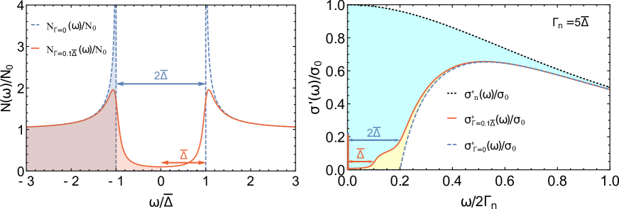
Figure 1: Comparison, at $T=0$, of a normal metal with two superconductors: a superconductor without pair-breaking processes ($\Gamma=0$) and a Dynes superconductor ($\Gamma=0.1\overline{\Delta}$). Left panel: density of states for both superconductors, normalized with respect to the constant normal-state density $N_{0}$. Shaded areas denote the occupied states. Right panel: real part of the optical conductivity $\sigma^{\prime}(\omega)$ for the normal metal and for both superconductors. The total scattering rate is $\Gamma_{n}=5\overline{\Delta}$ in all cases. Shaded areas show the weight which is missing in order to satisfy the sum rule Eq. (12). The missing weight is carried by the singular contribution to Eq. (8); this contribution is schematically shown as a bar at $\omega=0$.

A note about the vertex corrections is in place here. It is well known that, in general, in order to satisfy the Ward identities the vertex corrections should be present. However, in our case they do not appear, and the reasons are the same as in Refs. Nam67a, ; Fominov11, ; Kharitonov12, . First, in order to avoid the phase modulation of the superconducting order parameter,Ambegaokar61 we work in the transverse gauge. Second, since the impurity potential considered in Ref. Herman16, is point-like, also the normal-state vertex corrections to conductivity vanish in the CPA formalism.Velicky69 ; Elliott74

Nam has noticed that, when evaluating Eq. (6) within the Eliashberg theory, it is advantageous to replace the Eliashberg functions $Z(\omega)$ and $\Delta(\omega)$ with three complex functions: energy function $\epsilon(\omega)$, density of states $n(\omega)$, and density of pairs $p(\omega)$ defined by

$$\epsilon(\omega) = Z(\omega)\sqrt{\omega^{2}-\Delta^{2}(\omega)},$$

$$n(\omega) = \frac{\omega}{\sqrt{\omega^{2}-\Delta^{2}(\omega)}},$$

$$p(\omega) = \frac{\Delta(\omega)}{\sqrt{\omega^{2}-\Delta^{2}(\omega)}}.$$

Note that $n^{2}(\omega)-p^{2}(\omega)=1$ and there is some redundancy in this formulation. Taking into account that the square root is to be taken so that its imaginary part is positive, one can check readily the symmetry properties

$$\epsilon(-\omega)=-\epsilon^{\ast}(\omega),\quad n(-\omega)=n^{\ast}(\omega),\quad p(-\omega)=-p^{\ast}(\omega).$$

In terms of the functions $\epsilon(\omega)$, $n(\omega)$, and $p(\omega)$, the Nambu-Gor’kov Green’s function of the Eliashberg superconductors can be written as

$$\hat{G}({\bf k},\omega)=\frac{1}{2}\bigg{[}\frac{n(\omega)\tau_{0}+p(\omega)\tau_{1}+\tau_{3}}{\epsilon(\omega)-\varepsilon_{\bf k}}$$

$$+\frac{n(\omega)\tau_{0}+p(\omega)\tau_{1}-\tau_{3}}{\epsilon(\omega)+\varepsilon_{\bf k}}\bigg{]}.$$ (7)

Making use of Eq. (7), Nam has succeeded to express the optical conductivity in terms of the functions $n(\omega)$, $p(\omega)$, and $\epsilon(\omega)$. His result can be written in the following, slightly modified form:

$$\sigma(\omega)=\pi D\delta(\omega)+\sigma_{\rm reg}(\omega).$$ (8)

The first term describes the singular contribution of the condensate to frequency-dependent conductivity. Its magnitude can be written in terms of the superfluid density $n_{s}$ as $D=n_{s}e^{2}/m$ and is given by

$$\frac{D}{D_{0}}=\frac{n_{s}}{n}=-\int_{0}^{\infty}d\nu\tanh\left(\frac{\nu}{2T}\right){\rm Re}\left[\frac{p^{2}(\nu)}{\epsilon(\nu)}\right].$$ (9)

In the non-superconducting state obviously $D=n_{s}=0$.

The second term in Eq. (8) represents the non-singular part of the conductivity and is given byCarbotte05

$$\sigma_{\rm reg}(\omega)=\frac{iD_{0}}{\omega}\int_{-\infty}^{\infty}d\nu\tanh\left(\frac{\nu}{2T}\right)H(\nu+\omega,\nu),$$ (10)

where we have introduced an auxiliary complex function

$$H\big{(}x,y\big{)} = \frac{1+n(x)n^{*}(y)+p(x)p^{*}(y)}{2\left[\epsilon^{*}(y)-\epsilon(x)\right]},$$ (11)

$$+ \frac{1-n(x)n(y)-p(x)p(y)}{2\left[\epsilon(y)+\epsilon(x)\right]}.$$

The formulae Eqs. (8,9,10,11) are valid for any Eliashberg superconductor. It should be noted that for $\omega\rightarrow 0$, Eq. (10) predicts that $\sigma_{\rm reg}^{\prime\prime}(\omega)\approx D/\omega$, which describes the inductive response of the condensate.

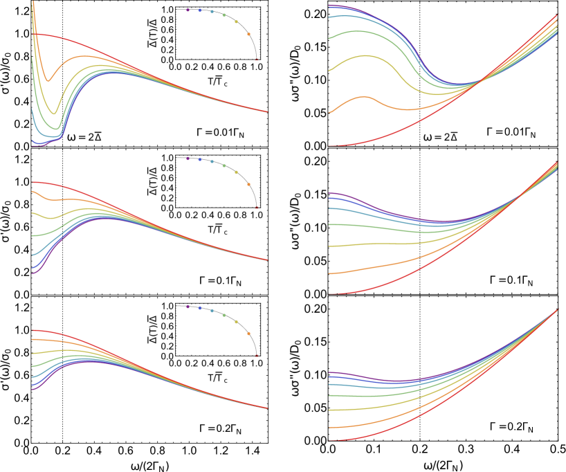
Figure 2: Frequency dependence of the real and imaginary parts of the conductivity Eq. (10) for the Dynes superconductors with fixed total scattering rate $\Gamma_{n}=5\overline{\Delta}$ and varying pair-breaking rates $\Gamma$. The temperature dependence of the gap, $\overline{\Delta}(T)$, was calculated using Eq. (15). The studied temperatures and the corresponding $\Gamma$-dependent values of $\overline{\Delta}(T)$ are presented in the insets. Note that, in all panels, the highest-temperature curves represent the normal state. The energy scale $2\overline{\Delta}$ is shown by the dotted lines. Let us point out that the values of $\omega\sigma^{\prime\prime}(\omega)/D_{0}$ at $\omega\rightarrow 0$ allow for a direct determination of the superfluid fraction $n_{s}/n$.

Before concluding this Section it is worth pointing out that Nam’s theory satisfies the conductivity sum rule

$$\int_{0}^{\infty}d\omega\sigma^{\prime}(\omega)=\frac{\pi}{2}D_{0}.$$ (12)

The proof of Eq. (12) makes use of two observations following from Eqs. (5,6): (i) the function $\sigma(\omega)$ satisfies the Kramers-Kronig relations, and (ii) the high-frequency limit of $\sigma^{\prime\prime}(\omega)$ is $D_{0}/\omega$. Writing down the Kramers-Kronig relation for $\sigma^{\prime\prime}(\omega)$ at $\omega\rightarrow\infty$, one recognizes easily that we arrive at Eq. (12).

III Optical conductivity: Dynes superconductors

Now we apply the general expressions from the previous Section to the Dynes superconductors, for which the energy function $\epsilon(\omega)$ is given by Eq. (3). The gap function $\Delta(\omega)$ of the Dynes superconductors is also known:Herman16

$$\Delta(\omega)=\frac{\omega}{\omega+i\Gamma}\overline{\Delta},$$ (13)

and this implies that

$$n(\omega)=\frac{\omega+i\Gamma}{\sqrt{(\omega+i\Gamma)^{2}-\overline{\Delta}^{2}}},\quad p(\omega)=\frac{\overline{\Delta}}{\sqrt{(\omega+i\Gamma)^{2}-\overline{\Delta}^{2}}}.$$ (14)

Typical frequency dependence of the real and imaginary parts of $n(\omega)$, $p(\omega)$, and $\epsilon(\omega)$ of a Dynes superconductor is shown in the Appendix. Equations (8,9,10,11) together with Eqs. (3,14) provide a complete description of the electromagnetic properties of the Dynes superconductors. Note that a single integration is required to determine the optical conductivity $\sigma(\omega)$, therefore the numerical cost is the same as in the widely used Mattis-Bardeen theory,Mattis58 which can be viewed as a special limit ($\Gamma=0$ and $\Gamma_{n}\gg\overline{\Delta}$) of the present approach.

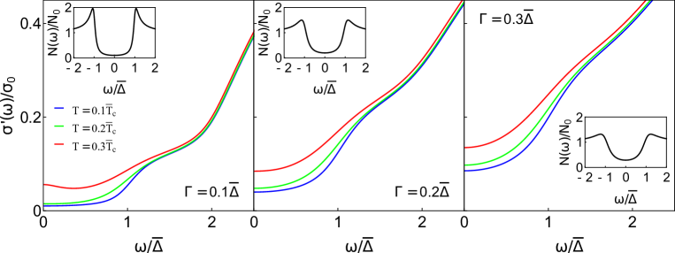
Figure 3: Frequency dependence of the dirty-limit conductivity $\sigma^{\prime}_{\rm reg}(\omega)$, Eq. (17), at low frequencies. For each considered value of the pair-breaking rate $\Gamma$ several temperatures are studied, and the corresponding Dynes density of states at $T=0$ is shown in the inset. The absorption edge at $\omega=\overline{\Delta}$ is clearly visible for $\Gamma\lesssim 0.3\overline{\Delta}$ and $T\lesssim 0.3\overline{T_{c}}$.

As shown in Ref. Herman16, , the magnitude of the gap $\overline{\Delta}$ of a Dynes superconductor is controlled by the pair-breaking scattering rate $\Gamma$, and in the BCS model with coupling constant $\lambda$ and cutoff frequency $\Omega$ it can be found by solving the self-consistent equation

$$\overline{\Delta}(T)=2\lambda\pi T\sum_{\omega_{n}>0}^{\Omega}\frac{\overline{\Delta}(T)}{\sqrt{(|\omega_{n}|+\Gamma)^{2}+\overline{\Delta}^{2}(T)}},$$ (15)

where the sum is taken over the Matsubara frequencies $\omega_{n}$. Starting with Eq. (15), we use the following notation: $\overline{\Delta}(T)$ denotes the gap at temperature $T$, whereas the $T=0$ value of the gap will be denoted simply as $\overline{\Delta}$. Moreover, the critical temperature of the dirty system will be called $\overline{T_{c}}$.

Before discussing the optical conductivity in the superconducting state, it is useful to start by analyzing the normal state $\overline{\Delta}=0$. In this case we have $\epsilon(\omega)=\omega+i\Gamma_{n}$, $n(\omega)=1$, and $p(\omega)=0$, and therefore the normal-state optical conductivity of a Dynes superconductor is given by the simple Drude formula

$$\sigma_{n}(\omega)=\frac{D_{0}}{2\Gamma_{n}-i\omega}.$$ (16)

Note that the relative weight of pair-breaking and pair-conserving processes is irrelevant in the normal state and therefore $\sigma_{n}(\omega)$ depends only on the total scattering rate $\Gamma_{n}$. In what follows we will measure the conductivities in terms of $\sigma_{0}=D_{0}/(2\Gamma_{n})$, which is the normal-state conductivity at $\omega=0$.

Our main goal is to study the change of the optical conductivity $\sigma(\omega)$ in the superconducting state at fixed $\Gamma_{n}$ for varying ratios of pair-conserving and pair-breaking processes. In Fig. 1 we plot $\sigma^{\prime}(\omega)$ of a moderately dirty Dynes superconductor with $\Gamma_{n}=5\overline{\Delta}$ at temperature $T=0$ for two values of the pair-breaking scattering rate $\Gamma$. In absence of pair-breaking, i.e. for $\Gamma=0$, our results are consistent with the Mattis-Bardeen theory generalized so as to apply for arbitrary values of $\Gamma_{s}$:Zimmermann91 for $\omega<2\overline{\Delta}$, the conductivity vanishes, whereas for $\omega\gg\overline{\Delta}$ it approaches the normal-state value. Note that already very small amount of pair-breaking $\Gamma=0.02\Gamma_{n}$ leads to dramatic changes of the low-frequency conductivity: even at the lowest frequencies, $\sigma^{\prime}_{\rm reg}(\omega)$ is finite, and in addition to the step at $\omega=2\overline{\Delta}$, optical conductivity also shows an additional step at $\omega=\overline{\Delta}$. Both of these results can be easily understood by inspecting the density of states of the Dynes superconductor, also shown in Fig. 1: similarly as in the normal metal, absorption at arbitrarily low frequencies is possible also in the Dynes superconductor, and the joint density of states increases at the two observed steps. Figure 2 shows that the filling in of the gap by pair-breaking processes quickly grows with $\Gamma$ and that the effect of pair breaking processes is quite similar to that of raising the temperature. As a result, the missing weight below the $\sigma^{\prime}_{n}(\omega)$ curve diminishes, resulting (due to the Ferrell-Glover-Tinkham sum ruleFerrell58 ) in quickly decreasing superfluid fraction $n_{s}/n$.

Dirty limit. The general formula Eq. (10) is somewhat difficult to interpret, but in the dirty limit, when $\Gamma_{s}\gg\overline{\Delta},\Gamma$, it can be simplified considerably. In fact, if we restrict ourselves to frequencies $\omega\ll\Gamma_{s}$, the function $\epsilon(\omega)$ reduces to $\epsilon(\omega)\approx i\Gamma_{n}$, and in this case Eq. (10) reduces to the physically much more transparent formulas

$$\sigma^{\prime}_{\rm reg}(\omega) = \frac{\sigma_{0}}{\omega}\int_{-\infty}^{\infty}d\nu\left[f(\nu)-f(\nu+\omega)\right]$$

$$\times \left[n^{\prime}(\nu)n^{\prime}(\nu+\omega)+p^{\prime}(\nu)p^{\prime}(\nu+\omega)\right],$$

$$\sigma^{\prime\prime}_{\rm reg}(\omega) = -\frac{\sigma_{0}}{\omega}\int_{-\infty}^{\infty}d\nu\left[1-2f(\nu)\right]$$ (17)

$$\times \left[n^{\prime}(\nu)n^{\prime\prime}(\nu+\omega)+p^{\prime}(\nu)p^{\prime\prime}(\nu+\omega)\right],$$

where $f(\nu)$ is the Fermi-Dirac distribution function. Similar expressions have been guessed without proof also in Ref. Zemlicka15, . The real part $\sigma^{\prime}_{\rm reg}(\omega)$ may be interpreted as a sum of contributions from the single-particle and Cooper-pair channels, both of which absorb the radiation in a semiconductor-like fashion. Note that, if one sets the pair-breaking rate $\Gamma$ to zero in Eqs. (17), one recovers a very compact form of the Mattis-Bardeen theory. It is also worth pointing out that the optical conductivity $\sigma_{\rm reg}(\omega)$ of course does depend, via $\sigma_{0}$, on the normal-state scattering rate $\Gamma_{n}$.

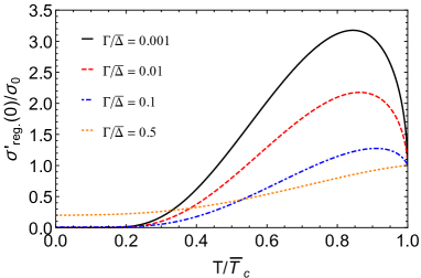
Figure 4: Temperature dependence of the dirty-limit conductivity $\sigma^{\prime}_{\rm reg}(0)$, Eq. (18), for several values of the pair-breaking scattering rate $\Gamma$.

An observation of the absorption edge at $\omega=\overline{\Delta}$ would provide a smoking gun for the concept of the Dynes superconductors. In order to identify the conditions under which this feature can be observable, in Fig. 3 we plot $\sigma^{\prime}_{\rm reg}(\omega)$ in the experimentally relevant dirty limit. One observes that the absorption edge at $\omega=\overline{\Delta}$ is clearly visible for $\Gamma\lesssim 0.3\overline{\Delta}$ and $T\lesssim 0.3\overline{T_{c}}$, thus rendering the concept of the Dynes superconductors experimentally falsifiable by optical means.

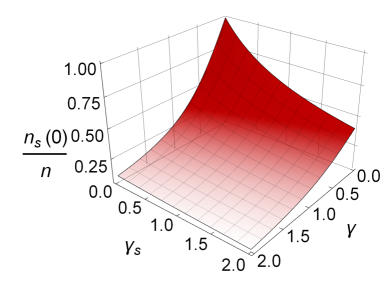
Figure 5: Superfluid fraction $n_{s}/n$ at $T=0$ as a function of the scattering rates $\gamma$ and $\gamma_{s}$ according to Eq. (21).

Coherence peak. It is well knownMarsiglio08 that in absence of pair breaking, the low-frequency conductivity $\sigma^{\prime}_{\rm reg}(\omega\rightarrow 0)$ diverges for all temperatures $T<T_{c}$. In this paragraph we will calculate $\sigma^{\prime}_{\rm reg}(0)$ for a Dynes superconductor, assuming that the dirty limit applies. We will show that $\sigma^{\prime}_{\rm reg}(0)$ stays finite, and that, as a function of temperature, it exhibits the well-known coherence peak with a magnitude controlled by $\Gamma$. To this end, let us make use of Eq. (17) which implies that

$$\frac{\sigma^{\prime}_{\rm reg}(0)}{\sigma_{0}}=\int_{0}^{\infty}\frac{dx}{2T\cosh^{2}(x/2T)}\left[n^{\prime}(x)^{2}+p^{\prime}(x)^{2}\right].$$ (18)

Results of the numerical evaluation of Eq. (18) are presented in Fig. 4. Note that, for sufficiently large pair-breaking rates $\Gamma$, the temperature dependence of $\sigma^{\prime}_{\rm reg}(0)$ is monotonic, without any coherence peaks. However, for sufficiently small $\Gamma$, the conductivity $\sigma^{\prime}_{\rm reg}(0)$ immediately below $T_{c}$ grows with decreasing temperature. In the vicinity of $T_{c}$, where $\overline{\Delta}$ is small, the growth is controlled by $\Gamma$, and for $\Gamma\ll T_{c}$ it can be shown that

$$\frac{\sigma^{\prime}_{\rm reg}(0)}{\sigma_{0}}=1+\frac{\pi}{8}\frac{\overline{\Delta}^{2}(T)}{\overline{T_{c}}\Gamma}.$$ (19)

When the temperature is decreased further, the thermal factor in Eq. (18) starts to dominate and $\sigma^{\prime}_{\rm reg}(0)$ decreases, until ultimately in the low-$T$ region it saturates at

$$\frac{\sigma^{\prime}_{\rm reg}(0)}{\sigma_{0}}=\frac{\Gamma^{2}}{\Gamma^{2}+\overline{\Delta}^{2}}.$$ (20)

The formula Eq. (20) is valid in the dirty limit for any ratio between $\Gamma$ and $\overline{\Delta}$. Note that the results Eqs. (19,20) can be used for a direct determination of the pair-breaking rate $\Gamma$ by microwave measurements.

Superfluid fraction. The superfluid fraction $n_{s}/n$ of a Dynes superconductor can be determined from Eq. (9). In the limit $T=0$, the integral can be taken analytically and, introducing dimensionless scattering rates $\gamma=\Gamma/{\overline{\Delta}}$ and $\gamma_{s}=\Gamma_{s}/{\overline{\Delta}}$, the result can be written as

$$\frac{n_{s}(0)}{n}=\begin{cases}\frac{1}{\gamma_{s}}\Bigg{[}\arctan(1/\gamma)-\frac{1}{\sqrt{1-\gamma_{s}^{2}}}\bigg{(}\arccos\gamma_{s}+\arctan\frac{\sqrt{1-\gamma_{s}^{2}}}{\gamma}-\arctan\frac{\sqrt{1-\gamma_{s}^{2}}\sqrt{\gamma^{2}+1}}{\gamma\gamma_{s}}\bigg{)}\Bigg{]}&\text{if }\gamma_{s}<1,\\ \frac{1}{\gamma_{s}}\Bigg{[}\arctan(1/\gamma)-\frac{1}{\sqrt{\gamma_{s}^{2}-1}}\ln\frac{\big{(}\gamma_{s}+\sqrt{\gamma_{s}^{2}-1}\big{)}\big{(}\gamma+\sqrt{\gamma_{s}^{2}-1}\big{)}}{\gamma\gamma_{s}+\sqrt{\gamma_{s}^{2}-1}\sqrt{\gamma^{2}+1}}\Bigg{]}&\text{if }\gamma_{s}\geq 1.\end{cases}$$ (21)

The formula Eq. (21) is somewhat cumbersome. In order to illustrate its meaning, in Fig. 5 we present a 3D plot of $n_{s}/n$ at $T=0$ as a function of $\gamma$ and $\gamma_{s}$. Notice that both types of scattering processes diminish the superfluid fraction, but (as expected) the pair-breaking impurities are much more effective in doing so. We have also checked that in absence of pair-breaking processes, i.e. for $\gamma=0$, Eq. (21) reduces to the previously published results.Nam67a ; Marsiglio08 ; Berlinsky93

For the sake of completeness let us also point out that, instead of using Eq. (9), at finite temperatures the superfluid fraction of a Dynes superconductor can be more conveniently calculated from the Matsubara sum

$$\frac{n_{s}(T)}{n}=2\pi T\sum_{\omega_{n}>0}\frac{\overline{\Delta}^{2}}{\Omega_{n}^{2}\left(\Omega_{n}+\Gamma_{s}\right)},$$ (22)

where $\Omega_{n}=\sqrt{(|\omega_{n}|+\Gamma)^{2}+\overline{\Delta}^{2}}$. Note that Eq. (22) can be obtained from the well-known result for superconductors in which only pair-conserving scattering is present,Nam67a ; Abrikosov63 provided one takes the pair-breaking processes into account by the minimal substitution $|\omega_{n}|\rightarrow|\omega_{n}|+\Gamma$, which was mentioned in the Introduction.

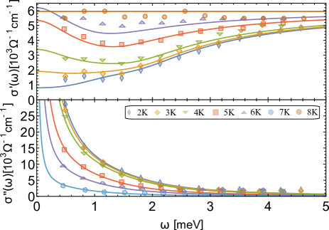
Figure 6: Real and imaginary parts of the optical conductivity for a $15.1$ nm thick MoN sample reported in Ref. Simmendinger16, . Fits of the data to the prediction for a dirty Dynes superconductor, Eqs. (17), are also shown. At $T=2$ K, the fits are three-parametric. For all curves at higher temperatures there is only one fitting parameter, namely $\overline{\Delta}(T)$.

IV Application to Molybdenum Nitride

Motivated by interest in the physics of the superconductor-insulator transition,Lin15 strongly disordered superconducting thin films have recently become the subject of intensive research. Since in-gap states are frequently observed in such systemsNoat13 ; Szabo16 ; Lin15 ; Cheng16 and since their tunneling density of states can be often described by the Dynes formula Eq. (1),Noat13 ; Szabo16 the theory developed in this paper should be directly applicable precisely to such systems. It is also fortunate that, due to progress in terahertz spectroscopy, high-quality optical data on strongly disordered superconductors have recently become available.Cheng16 ; Simmendinger16

As an example, in this paper we have chosen to discuss the terahertz spectra obtained by Simmendinger et al. on molybdenum nitride (MoN) thin films in Ref. Simmendinger16, . The authors have studied a whole series of films with different thickness, but most details were presented for the 15.1 nm thick film, and we will test the predictions of our theory against this sample.

Simmendinger et al. start their analysis by noting that although their films are definitely deeply in the dirty limit, the Mattis-Bardeen theory can not fit their data. The reason is that even at the lowest temperatures, large in-gap absorption has been observed. In Ref. Simmendinger16, this finding has been explained by the existence of a hypothetical parallel normal-conducting channel inside the sample. While this might be possible - although one would have to explain the absence of an internal proximity coupling between the normal channel and the superconducting channel - we consider here an alternative explanation, namely that MoN is a Dynes superconductor.

We proceed as follows: since the studied sample is obviously in the extremely dirty limit, we can use Eqs. (17) to fit the observed frequency dependence of the real and imaginary parts of conductivity. At the lowest experimental temperature $T=2$ K the least-squares fitting procedure is robust and we can safely fix the three free parameters entering Eqs. (17), namely the overall scale $\sigma_{0}$, the superconducting gap $\overline{\Delta}$, and the pair-breaking scattering rate $\Gamma$. The resulting fit is shown in Fig. 6; the agreement between theory and experiment is seen to be reasonable.

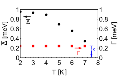
Figure 7: Temperature dependence of the gap parameter $\overline{\Delta}(T)$ obtained from the fits shown in Fig. 6. Also shown is the value of $\Gamma$ which has been determined at the lowest temperature $T=2$ K; at higher temperatures its value was kept fixed.

Next we assume that both $\sigma_{0}$ and $\Gamma$ do not depend on temperature, and using their values which have been determined at $T=2$ K, we fit the higher-temperature conductivity data by a single parameter: the superconducting gap $\overline{\Delta}(T)$. The resulting temperature dependence of the superconducting gap $\overline{\Delta}(T)$ exhibits the expected order parameter-like shape, see Fig. 7, and the corresponding fits of the optical conductivity are shown in Fig. 6. The agreement between experiment and theory is satisfactory, especially if we realize that the fits of two frequency-dependent functions $\sigma^{\prime}_{\rm reg}(\omega)$ and $\sigma^{\prime\prime}_{\rm reg}(\omega)$ are done using a single free parameter $\overline{\Delta}(T)$ at every temperature $T>2$ K.

Note that our estimate of the pair-breaking rate of the 15.1 nm thick MoN film, $\Gamma\approx 0.2$ meV, is of the same order of magnitude as $\Gamma\approx 0.1$ meV directly measured by tunneling in a similar 10 nm thick MoC film.Szabo16 It is worth pointing out that such values are reasonable. In fact, according to our interpretation, $\Gamma$ is a typical exchange field inside the superconducting film. If we assume that the magnetic impurities are located in the vicinity of the film/substrate interface with area density $n_{\Box}$, and if we characterize the impurities by exchange field $J$ decaying to zero on the length scale $a$ (of atomic dimensions), then we can make the following very rough estimate: $\Gamma\approx Ja^{3}n_{\Box}/d$. Let us take the typical values $J=1$ eV, $a=0.3$ nm, and for the film thickness $d=15.1$ nm. If we assume that $n_{\Box}=x/a^{2}$ (where $x$ is the fraction of atomic positions occupied by magnetic impurities), then we obtain that $\Gamma\approx 0.2$ meV corresponds to $x=0.01$, which looks quite reasonable. Larger values of $a$ lead to even smaller concentrations of the magnetic impurities.

V Conclusions

Based on Nam’s description of the electromagnetic properties of superconductors,Nam67a in this paper we have presented a comprehensive set of predictions for the optical conductivity of the recently identified Dynes superconductors.Herman16 ; Herman17 In particular, we have shown that two metals with the same optical response in the normal state and equal superconducting gaps $\overline{\Delta}$ may exhibit very different superconducting responses, with the shape of the latter depending on the ratio of the pair-breaking and pair-conserving scattering rates $\Gamma$ and $\Gamma_{s}$, see Fig. 2.

The most characteristic optical fingerprint of a Dynes superconductor is the presence (at low temperatures and for physically reasonable pair-breaking rates) of an additional absorption edge in $\sigma^{\prime}(\omega)$ at $\omega=\overline{\Delta}$, which exists in addition to the conventional absorption edge at $\omega=2\overline{\Delta}$. Another property which is unique to a Dynes superconductor is that the dissipative component of the low-frequency conductivity $\sigma^{\prime}_{\rm reg}(\omega\rightarrow 0)$ stays finite down to temperature $T=0$. Both of these anomalies are in fact a simple consequence of the fact that the Dynes superconductors are gapless, see Fig. 1.

Furthermore we have shown that the pair-breaking scattering rate $\Gamma$ can be straightforwardly determined from microwave measurements, either from the slope of the coherence peak, Eq. (19), or from the low-frequency conductivity $\sigma^{\prime}_{\rm reg}(\omega\rightarrow 0)$ in the limit of low temperatures, Eq. (20), thus enabling comparison with the $\Gamma$ values obtained from the tunneling spectroscopy.

Practical formulae have been derived for the superfluid fraction $n_{s}/n$ (or, equivalently, superfluid stiffness) of the Dynes superconductors. In the zero-temperature limit, we have found an explicit algebraic expression, Eq. (21), showing how $n_{s}(0)/n$ depends on the scattering rates $\Gamma$ and $\Gamma_{s}$. At finite temperatures, the formula Eq. (22), which is suitable for an efficient numerical evaluation of $n_{s}(T)/n$, has been derived.

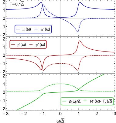
Figure 8: The real and imaginary parts of the functions $n(\omega)$, $p(\omega)$, and $\epsilon(\omega)$ describing a Dynes superconductor with the pair-breaking rate $\Gamma=0.1\overline{\Delta}$.

Strongly disordered thin superconducting films seem to be the best candidate where the Dynes phenomenology may be observable.Szabo16 ; Noat13 This is probably caused by the presence of magnetic impurities at the interface between the film and the substrate, which may be present even in otherwise very clean films.Casalbuoni05 ; Junginger17 In this paper we have shown that the apparently anomalous optical data for MoN thin filmsSimmendinger16 can be reasonably fitted by the Dynes optics, see Figs. 6,7. This result lends further support to the identification of strongly disordered thin superconducting films as potential Dynes superconductors.

From the methodological point of view, we would like to point out that Eqs. (8,9,10,11) together with Eqs. (3,14) provide a complete description of the electromagnetic properties of the Dynes superconductors. Their numerical evaluation is equally costly as that which makes use of the generalized Mattis-Bardeen formula,Zimmermann91 but, unlike the latter, allows also for pair-breaking processes. As regards the formal properties of our results, the optical conductivity Eq. (8) has the correct analytic properties and high-frequency asymptotics, and therefore it satisfies also the conductivity sum rule Eq. (12). Moreover, by scanning a wide range of parameters $\overline{\Delta}$, $\Gamma_{s}$, and $\Gamma$, we have checked that $\sigma^{\prime}(\omega)$ for a Dynes superconductor is positive definite (as it should be), although we were not able to prove it. This means that our theory for optics of the Dynes superconductors satisfies the same set of constraints which is obeyed by the simple Drude formula. Since the latter is known to be a good starting point when analyzing the optics of normal metals, we are convinced that the present theory might play an analogous role in the superconducting state.

*

Appendix A The functions $n(\omega)$, $p(\omega)$, and $\epsilon(\omega)$

For readers’ convenience, in Fig. 8 we plot the functions $n(\omega)=n^{\prime}(\omega)+in^{\prime\prime}(\omega)$ and $p(\omega)=p^{\prime}(\omega)+ip^{\prime\prime}(\omega)$ for a Dynes superconductor, defined by Eq. (14). When frequency is measured in units of $\overline{\Delta}$, these functions depend on a single parameter: the pair-breaking rate $\Gamma$. Also shown in Fig. 8 are the real and imaginary parts of the function $\epsilon(\omega)$ defined by Eq. (3).

References

- (1) P. W. Anderson, J. Phys. Chem. Solids 11, 26 (1959). It should be pointed out that Anderson’s argument has its limitations: sufficiently strong nonmagnetic disorder can lead to a superconductor to insulator transition.
- (2) A. A. Abrikosov and L. P. Gor’kov, Sov. Phys. JETP 12, 1243 (1961).
- (3) R. C. Dynes, V. Narayanamurti, and J. P. Garno, Phys. Rev. Lett. 41, 1509 (1978).
- (4) Y. Noat, V. Cherkez, C. Brun, T. Cren, C. Carbillet, F. Debontridder, K. Ilin, M. Siegel, A. Semenov, H.-W. H bers, and D. Roditchev, Phys. Rev. B 88, 014503 (2013).
- (5) P. Szabó, T. Samuely, V. Hašková, J. Kačmarčík, M. Žemlička, M. Grajcar, J. G. Rodrigo, and P. Samuely, Phys. Rev. B 93, 014505 (2016).
- (6) F. Herman and R. Hlubina, Phys. Rev. B 94, 144508 (2016).
- (7) F. Herman and R. Hlubina, Phys. Rev. B 95, 094514 (2017).
- (8) T. Kondo, W. Malaeb, Y. Ishida, T. Sasagawa, H. Sakamoto, Tsunehiro Takeuchi, T. Tohyama, and S. Shin, Nat. Commun. 6, 7699 (2015).
- (9) D. C. Mattis and J. Bardeen, Phys. Rev. 111, 412 (1958).
- (10) S. B. Nam, Phys. Rev. 156, 470 (1967).
- (11) S. B. Nam, Phys. Rev. 156, 487 (1967).
- (12) J. P. Carbotte, E. Schachinger, and J. Hwang, Phys. Rev. B 71, 054506 (2005).
- (13) C. J. J. Coumou, E. F. C. Driessen, J. Bueno, C. Chapelier, and T. M. Klapwijk, Phys. Rev. B 88, 180505(R) (2013).
- (14) M. Žemlička, P. Neilinger, M. Trgala, M. Rehák, D. Manca, M. Grajcar, Phys. Rev. B 92, 224506 (2015).
- (15) V. G. Kogan, R. Prozorov, and V. Mishra, Phys. Rev. B 88, 224508 (2013).
- (16) Ya.V. Fominov, M. Houzet, and L.I. Glazman, PRB 84, 224517 (2011).
- (17) M. Kharitonov, T. Proslier, A. Glatz, and M.J. Pellin, PRB 86, 024514 (2012).
- (18) F. M. Marchetti and B. D. Simons, J. Phys. A 35, 4201 (2002).
- (19) H. Shiba, Prog. Theor. Phys. 40, 435 (1968).
- (20) Julian Simmendinger, Uwe S. Pracht, Lena Daschke, Thomas Proslier, Jeffrey A. Klug, Martin Dressel, Marc Scheffler, Phys. Rev. B 94, 064506 (2016).
- (21) F. Marsiglio and J. P. Carbotte, in Superconductivity, K. H. Bennemann and J. B. Ketterson, Eds., Vol. I, Springer, Berlin, 2008.
- (22) G.Rickayzen, Green’s Functions and Condensed Matter, Academic Press, New York, 1980.
- (23) V. Ambegaokar and L.P. Kadanoff, Nuovo Cimento 22, 914 (1961).
- (24) B. Velický, Phys. Rev. 184, 614 (1969).
- (25) R.J. Elliott, J. A. Krumhansl, and P.L. Leath, Rev. Mod. Phys. 46, 465 (1974).
- (26) W. Zimmermann, E. Brandt, M. Bauer, E. Seider, and L. Genzel, Physica C 183, 99 (1991).
- (27) R. A. Ferrell and R. E. Glover, Phys. Rev. 109, 1398 (1958), M. Tinkham and R. A. Ferrell, Phys. Rev. Lett. 2, 331 (1959).
- (28) A. J. Berlinsky, C. Kallin, G. Rose, and A.-C. Shi, Phys. Rev. B 48, 4074 (1993).
- (29) A. A. Abrikosov, L. P. Gor’kov, and I. E. Dzyaloshinskii, Methods of Quantum Field Theory in Statistical Physics (Prentice-Hall, Englewood Cliffs, NJ, 1963).
- (30) Yen-Hsiang Lin, J. Nelson, and A. M. Goldman, Physica C 514, 130 (2015).
- (31) Bing Cheng, Liang Wu, N. J. Laurita, Harkirat Singh, Madhavi Chand, Pratap Raychaudhuri, N. P. Armitage, Phys. Rev. B 93, 180511 (2016).
- (32) S. Casalbuoni, E.A. Knabbe, J. Kötzler, L. Lilje, L. von Sawilski, P. Schmüser, and B. Steffen, Nuclear Instruments and Methods in Physics Research A 538, 45 (2005).
- (33) T. Junginger, S. Calatroni, A. Sublet, G. Terenziani, T. Prokscha, Z. Salman, T. Proslier, J. Zasadzinski, preprint arXiv:1703.08635.