Abstract

In this paper, we investigate the main algebraic properties of the maximally superintegrable system known as “Perlick system type I”. All possible values of the relevant parameters, $K$ and $\beta$, are considered. In particular, depending on the sign of the parameter $K$ entering in the metrics, the motion will take place on compact or non compact Riemannian manifolds. To perform our analysis we follow a classical variant of the so called factorization method. Accordingly, we derive the full set of constants of motion and construct their Poisson algebra. As it is expected for maximally superintegrable systems, the algebraic structure will actually shed light also on the geometric features of the trajectories, that will be depicted for different values of the initial data and of the parameters. Especially, the crucial role played by the rational parameter $\beta$ will be seen “in action”.

PACS: 04.20.-q; 02.40.Ky; 02.30.Ik

KEYWORDS: Bertrand spaces, superintegrable systems, factorization method, constants of motion.

1 Introduction

The Perlick systems type I and II have been studied in a large number of papers, where several crucial features have been discovered (see for instance [2, 3, 4, 5, 6, 7, 8, 9, 10, 11]). In particular, let us remind that in his original paper [2], V. Perlick constructed the most general class of three-dimensional spherically symmetric lagrangian systems complying with the requirements of the celebrated Bertrand’s Theorem [12], namely the fact that they possess stable circular orbits and all bounded trajectories are closed. Of course he had to abandon the Euclidean space framework in favour of more general conformally flat manifolds. In this way he unveiled the deep connection existing between the metrics characterizing the manifold and the corresponding integrable potentials. He classified these generalized Bertrand systems in two multiparametric families, defined according to their Euclidean limit. Family I is the one yielding the Kepler-Coulomb system and Family II is the one leading to the radial harmonic oscillator [13, 14, 15]. In ref. [4] by means of the coalgebra approach the extension to hyperspherically symmetric systems in any dimension was performed, and an intrinsic characterization of the two families was proposed. Family I was denoted as “intrinsic Kepler-Coulomb” because, up to additive and multiplicative constants (one could say, “up to affine transformations”), the pertaining class of potentials were discovered to be just the Green’s functions of the corresponding Laplace-Beltrami operators. Analogously, the potentials comprised in Family II, again up to affine transformations, were identified as the “inverse-squared” of those belonging to Family I and these have been called “intrinsic oscillator”. In a subsequent paper [5] the same authors gave a rigorous proof of the previously obtained results, including that of the periodicity of the bounded motions, and provided a closed expression for the corresponding trajectories. Thus, Perlick’s systems of type I and II are the most general classes of “maximally superintegrable” lagrangian (and consequently Hamiltonian) systems with (hyper-)spherical symmetry.

To further clarify our previous statements, let us recall that a classical Hamiltonian system with $n$ degrees of freedom is said to be integrable if there are $n$ functionally independent globally defined and single-valued integrals of motion in involution for a given Poisson bracket. If there exist $k$, with $0<k\leq n-1$, additional integrals (they must be functionally independent, but not all of them in involution) it is called superintegrable. When $k=n-1$, the system is maximally superintegrable. In this case, all bounded trajectories are closed and the motion is periodic [16, 17, 18]. The constants of motion of maximally superintegrable systems close an algebra and can be used to determine the trajectories in pure algebraic way. Kepler-Coulomb and (isotropic) harmonic oscillator systems are examples of spherically symmetric and maximally superintegrable systems in an $n$ dimensional Euclidean space. In dealing here with a maximally superintegrable system such as Perlick system of type I, rather than relying on an analytic approach one as in [5], we will follow an algebraic one, that can be generally called “factorization approach” or “factorization method”. Through the factorization method the algebra of the integrals of motions can be explicitly constructed, and its features will pave the way to identifying relevant geometric properties such as the shape of the closed orbits. We wish to remark that the factorization method applies both to classical and quantum systems. The method is quite simple in yielding the constants of motion (symmetries) and unveiling their underlying algebra [19, 20, 21, 22, 23, 24, 25, 26]. We should mention that other methods have been successfully applied to find the constants of motion of superintegrable systems. One of them is based on the Hamilton-Jacobi equation, as it is shown in many references [15, 27, 28]. Another interesting way to look for constants of motion is the method of coalgebras developed in [29, 30]. A systematic algebraic method has also been used in other papers [31, 32]. In this work, we will perform a systematic investigation of the constants of motion of the classical superintegrable three dimensional Perlick system type I by using the factorization method in order to derive the trajectories in a purely algebraic way.

This paper is organized as follows. In section 2, we briefly recall the basic definition of the Perlick system of type I which depends essentially on two parameters $\beta$ and $K$. We will introduce new variables more suitable to describe the compact or non compact manifolds where this system may be defined. In section 3, we construct the constants of motion by means of an extension of the factorization method to classical three dimensional systems (it can be applied to higher dimensions too). The trajectories of Perlick I system are derived, discussed and depicted, for different values of the initial conditions as well as of the relevant parameters of the system, i.e, $K$ and $\beta=m/n$. Both open and closed trajectories are presented. The crucial point of the whole treatment, namely the evaluation of the algebra of the constants of motion is also given here. Section 4 is devoted to the special case of the motion in the plane. The key role played by the requirement that $\beta$ be a rational number becomes extremely clear in this somehow simplified setting. Finally, in section 5, we summarize the new results that we have obtained, emphasizing what are in our opinion the most relevant ones. As a closing comment, we will briefly outline the most promising developments.

2 The Perlick system type I

The Hamiltonian for the Perlick system type I in spherical coordinates $(r,\theta,\varphi)$ is

$$\widetilde{H}^{\pm}=\beta^{2}(1+K\,r^{2})\,\dfrac{p_{r}^{2}}{2}+\dfrac{{\bf L}^{2}}{2\,r^{2}}+G\pm\dfrac{1}{r}\,\sqrt{1+K\,r^{2}}\,,$$ (2.1)

where ${\bf L}$ is the angular momentum and ${\bf L}^{2}$ can be considered as an angular Hamiltonian $H_{\theta\varphi}$ in the variables $(\theta,\varphi)$, having the form

$${\bf L}^{2}=H_{\theta\varphi}=p_{\theta}^{2}+\dfrac{p_{\varphi}^{2}}{\sin^{2}{\theta}}\,$$ (2.2)

being $K$, $G$ real constants and $\beta=m/n$ a rational number. We can also consider $p_{\varphi}^{2}$ as a free Hamiltonian $H_{\varphi}$ in the variables $(\varphi,p_{\varphi})$, defined on the unit circle. The angular variables have the usual range: $0\leq\theta\leq\pi$ and $0\leq\varphi<2\pi$. The radial variable has different ranges depending on $K$. If $K\geq 0$, then $0<r<\infty$, while if $K<0$, $r$ must be restricted to the finite interval $0<r<1/\sqrt{-K}$. In his paper [2] Perlick considered only the negative sign in front of the square root of the potential, that is $\widetilde{H}^{-}$, in order to have bounded motions. However, we will show that for the case $K<0$ both Hamiltonians $\widetilde{H}^{\pm}$ should be taken into account in order to have a well defined Hamiltonian on a three dimensional sphere. The metric associated to this Hamiltonian is [4]

$$ds^{2}=\frac{dr^{2}}{\beta^{2}\,(1+K\,r^{2})}+r^{2}\,(d\theta^{2}+\sin^{2}\theta\,d\varphi^{2})\,.$$ (2.3)

Another point of view on the Hamiltonians (2.1) is to look at them not as defined in a curved space but as position dependent mass Hamiltonians in a flat space [33, 34].

Since $\{{\bf L}^{2},\widetilde{H}^{\pm}\}=0$, ${\bf L}^{2}$ is a constant of motion and takes the positive values ${\bf L}^{2}=\ell^{2}$. Here, $\{\cdot,\cdot\}$ stands for the Poisson brackets (PBs) that for the functions $f(r,\theta,\phi),\,g(r,\theta,\varphi)$ in spherical coordinates are defined by

$$\{f,g\}=\dfrac{\partial f}{\partial r}\dfrac{\partial g}{\partial p_{r}}-\dfrac{\partial f}{\partial p_{r}}\dfrac{\partial g}{\partial r}+\dfrac{\partial f}{\partial\theta}\dfrac{\partial g}{\partial p_{\theta}}-\dfrac{\partial f}{\partial p_{\theta}}\dfrac{\partial g}{\partial\theta}+\dfrac{\partial f}{\partial\varphi}\dfrac{\partial g}{\partial p_{\varphi}}-\dfrac{\partial f}{\partial p_{\varphi}}\dfrac{\partial g}{\partial\varphi}\,.$$ (2.4)

For the sake of simplicity, we also choose $G=0$, so when we replace ${\bf L}^{2}$ by its constant value $\ell^{2}$ we can rewrite the initial Hamiltonian (2.1) as an effective Hamiltonian $\widetilde{H}_{r}^{\pm}$ in the variable $r$:

$$\widetilde{H}_{r}^{\pm}=\beta^{2}(1+K\,r^{2})\,\dfrac{p_{r}^{2}}{2}+\dfrac{\ell^{2}}{2\,r^{2}}\pm\dfrac{1}{r}\,\sqrt{1+K\,r^{2}}\,.$$ (2.5)

Since $\{p_{\varphi},\widetilde{H}^{\pm}\}=0$, $p_{\varphi}$ is another constant of motion: $p_{\varphi}=\ell_{z}=const$. In the same way, after replacing $H_{\varphi}$ by $\ell_{z}$ in (2.2), we have an effective Hamiltonian $H_{\theta}$ in $\theta$:

$$H_{\theta}=p_{\theta}^{2}+\dfrac{\ell_{z}^{2}}{\sin^{2}{\theta}}\,.$$ (2.6)

Notice that $H_{\theta}$ is singular at the angles $\theta=0$ and $\theta=\pi$, so the trajectories lie between these two values (i.e. the North and South poles cannot be reached unless $\ell_{z}=0$). Once fixed the values of $\ell,\ell_{z}$, the turning points for $\theta$ are given by the solutions of $\ell^{2}={\ell_{z}^{2}}/{\sin^{2}{\theta}}$.

In order to take into account different signs and values of $K$, we will make use of the ${\kappa}$-dependent cosine and sine functions defined by

$${\rm\ \!C}_{\kappa}(u)\equiv\left\{\begin{array}[]{ll}\cos{\sqrt{{\kappa}}\,u}&\quad{\kappa}>0\\ \qquad 1&\quad{\kappa}=0\\ \cosh{\sqrt{-{\kappa}}\,u}&\quad{\kappa}<0\end{array}\right.,\quad{\rm\ \!S}_{\kappa}(u)\equiv\left\{\begin{array}[]{ll}\frac{1}{\sqrt{{\kappa}}}\sin{\sqrt{{\kappa}}\,u}&\quad{\kappa}>0\\ \qquad u&\quad{\kappa}=0\\ \frac{1}{\sqrt{-{\kappa}}}\sinh{\sqrt{-{\kappa}}\,u}&\quad{\kappa}<0\end{array}\right..$$ (2.7)

The ${\kappa}$-tangent is defined by

$${\rm\ \!T}_{\kappa}(u)\equiv\frac{{\rm\ \!S}_{\kappa}(u)}{{\rm\ \!C}_{\kappa}(u)}\,.$$

Some relations among these ${\kappa}$-functions are [36, 37]:

$${\rm\ \!C}_{\kappa}^{2}(u)+{\kappa}{\rm\ \!S}_{\kappa}^{2}(u)=1,\qquad\frac{{\rm d}}{{\rm d}u}{\rm\ \!C}_{\kappa}(u)=-{\kappa}{\rm\ \!S}_{\kappa}(u),\qquad\frac{{\rm d}}{{\rm d}u}{\rm\ \!S}_{\kappa}(u)={\rm\ \!C}_{\kappa}(u)\,.$$ (2.8)

Now, let us introduce the parameter $\kappa$ instead of $K$ and make the following change of canonical variables,

$$K=-\kappa\,,\qquad r={\rm\ \!S}_{\kappa}(\xi),\qquad p_{r}=\frac{p_{\xi}}{{\rm\ \!C}_{\kappa}(\xi)}\,,$$ (2.9)

where the range of $\xi$ is as follows: (a) for ${\kappa}\leq 0$, $0<\xi<\infty$; (b) for $\kappa>0$, we have two natural choices: $0<\xi<\pi/(2\sqrt{{\kappa}})$ or $\pi/(2\sqrt{{\kappa}})<\xi<\pi/\sqrt{{\kappa}})$. This change of coordinates can be interpreted in the following way. The variables $(\xi,\theta,\varphi)$ can be considered as the angular coordinates of the points of a (pseudo) sphere in $\mathbb{R}^{4}$. When ${\kappa}<0$ they parametrize the points of one sheet of a three dimensional (3D) hyperboloid; when ${\kappa}=0$ the coordinates $(\xi,\theta,\varphi)$ represent the spherical coordinates of the points of $\mathbb{R}^{3}$; finally, for ${\kappa}>0$ these variables with $0<\xi<\pi/(2\sqrt{{\kappa}})$ parametrize the points of one half (the north hemisphere) of a deformed 3D sphere, and the values $\pi/(2\sqrt{{\kappa}})<\xi<\pi/\sqrt{{\kappa}}$ give the points of the south hemisphere. In the case ${\kappa}<0$, this choice of coordinates is not important since the north and south hemispheres of a hyperboloid are not connected and can be taken independently without any problem, but in the case ${\kappa}>0$ this parametrization of the points of a sphere is quite relevant.

Next, we introduce a Hamiltonian $H$ in the variables $(\xi,\theta,\varphi)$ defined as follows for any value of ${\kappa}$:

$$H(\xi,\theta,\varphi)=\beta^{2}\,\dfrac{p_{\xi}^{2}}{2}+\dfrac{{\bf L}^{2}}{2}\frac{1}{{\rm\ \!S}_{\kappa}^{2}(\xi)}-\frac{1}{{\rm\ \!T}_{\kappa}(\xi)}\,,$$ (2.10)

and the corresponding effective Hamiltonian $H_{\xi}$ by

$$H_{\xi}=\beta^{2}\,\dfrac{p_{\xi}^{2}}{2}+\dfrac{{\ell}^{2}}{2}\frac{1}{{\rm\ \!S}_{\kappa}^{2}(\xi)}-\frac{1}{{\rm\ \!T}_{\kappa}(\xi)}=\beta^{2}\,\dfrac{p_{\xi}^{2}}{2}+V_{\rm eff}({\xi})\,.$$ (2.11)

We will see the relation of this Hamiltonian with the Perlick Hamiltonians $\widetilde{H}^{\pm}$ for different values of ${\kappa}$.

• ${\kappa}\leq 0$. In this case, both variables $\xi$ and $r$ vary in the positive semi-line $(0,\infty)$. If we change the variables in (2.1) according to (2.9) it is easy to check that

  $$H(\xi,\theta,\varphi)=\widetilde{H}^{-}(r,\theta,\varphi)\,.$$ (2.12)

• ${\kappa}>0$. Here, there are two complementary intervals for the range of variable $\xi$ as mentioned above. If we change the variables in (2.1) according to (2.9) we get

  $$H(\xi,\theta,\varphi)=\left\{\begin{array}[]{ll}\widetilde{H}^{-}(r,\theta,\varphi)\,,&0<\xi<\dfrac{\pi}{2\sqrt{{\kappa}}}\,,\qquad 0<r<\dfrac{1}{\sqrt{{\kappa}}},\\[10.76385pt] \widetilde{H}^{+}(r,\theta,\varphi)\,,&\dfrac{\pi}{2\sqrt{{\kappa}}}<\xi<\dfrac{\pi}{\sqrt{{\kappa}}}\,,\qquad\dfrac{1}{\sqrt{{\kappa}}}>r>0\,.\end{array}\right.$$ (2.13)

  Therefore, in this case we have a unique Hamiltonian $H$ well defined for all the points of the sphere $0<\xi<{\pi}/{\sqrt{{\kappa}}}$, such that on the north hemisphere is described by $\widetilde{H}^{-}$ and on the south by $\widetilde{H}^{+}$. When these points are parametrized in terms of $(r,\theta,\varphi)$ variables, each hemisphere gives rise to the two distinct Hamiltonians $\widetilde{H}^{\pm}$. This is very important since in general the trajectories on the sphere are not restricted to the upper or the lower hemispheres, and a full description of all of them should be done by means of $H$.

Henceforth, we will use the following notation. For all the values of ${\kappa}$ we will take the Hamiltonian $H(\xi,\theta,\varphi)$ as given in (2.10) or the effective Hamiltonian $H_{\xi}(\xi)$ in (2.11). The ranges of the variable $\xi$ are taken according to the previous discussion depending on the values of ${\kappa}$, in particular for ${\kappa}>0$ the interval is $0<\xi<\frac{\pi}{\sqrt{{\kappa}}}$.

3 Constants of motion from factorization properties

In this model, we already have three independent constants of motion: $H,H_{\theta\varphi},H_{\varphi}$ with constant values given by $E,\ell^{2},\ell_{z}^{2}$. Our aim is to find additional constants of motion by means of the factorization method in order to show the maximal superintegrability of the system. A first pair of constants $X^{\pm}$ will be obtained from the effective Hamiltonians $H_{\xi}$ and $H_{\theta}$, and a second pair $Y^{\pm}$ from the next two effective Hamiltonians, $H_{\theta}$ and $H_{\varphi}$.

3.1 The constants of motion $X^{\pm}$

The first set of constants $X^{\pm}$ are constructed in terms of the shift functions of $H_{\xi}$ and the ladder functions of $H_{\theta}$ which are obtained as follows [19].

• Shift functions of $H_{\xi}$

  The Hamiltonian (2.11) can be factorized as

  $$H_{\xi}=B^{+}B^{-}+\lambda_{\xi}\,,$$ (3.1)

  where

  $$B^{\pm}=\frac{1}{\sqrt{2}}\,\left(\mp\,i\,{\beta}\,{p_{\xi}}+\frac{\ell}{{\rm\ \!T}_{\kappa}{(\xi)}}-\dfrac{1}{\ell}\right)\,,\qquad\lambda_{\xi}=-\dfrac{1}{2}\left(\dfrac{1}{\ell^{2}}-{\kappa}\,\ell^{2}\right)\,.$$ (3.2)

  The shift functions $B^{\pm}$ are complex conjugate of each other and they satisfy the following PBs together with the Hamiltonian $H_{\xi}$

  $$\{B^{-},B^{+}\}=i\,\beta\,\dfrac{\ell}{{{\rm\ \!S}_{\kappa}}^{2}(\xi)}\,,\qquad\{H_{\xi},B^{\pm}\}=\pm i\,\beta\,\dfrac{\ell}{{{\rm\ \!S}_{\kappa}}^{2}(\xi)}\,B^{\pm}\,.$$ (3.3)

  The second PB of (3.3) implies that

  $$\{H,B^{\pm}\}=\pm i\,\beta\,\dfrac{\sqrt{H_{\theta\varphi}}}{{{\rm\ \!S}_{\kappa}}^{2}(\xi)}\,B^{\pm}\,.$$ (3.4)

  From the factorization given in (3.1) or the effective potential (2.11), we conclude that the energy $E$ of the total Hamiltonian $H_{\xi}$ for bounded motions must satisfy the following inequalities depending on ${\kappa}$:

  $$\begin{array}[]{ll}{\kappa}<0\,,&-\sqrt{|{\kappa}|}>E\geq-\dfrac{1}{2}\left(\dfrac{1}{\ell^{2}}+|{\kappa}|\ell^{2}\right)\,,\\[8.61108pt] {\kappa}=0\,,&0>E\geq-\dfrac{1}{2\,\ell^{2}}\,,\\[8.61108pt] {\kappa}>0\,,&\infty>E\geq-\dfrac{1}{2}\left(\dfrac{1}{\ell^{2}}-{\kappa}\ell^{2}\right)\,.\end{array}$$ (3.5)

  In Fig. 1, it is shown the effective potential $V_{\rm eff}({\xi})$ given by (2.11) together with the conditions on the energy (3.5) for different values of ${\kappa}$. For all these three cases, bounded motions have two turning points in the variable $\xi$ given by $E=V_{\rm eff}({\xi})$. For $E\geq-\sqrt{|{\kappa}|}$ the trajectory will be unbounded with only one turning point for ${\kappa}\leq 0$.

  

  

  

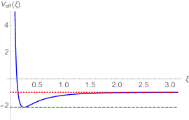
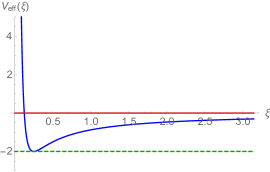
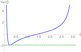
  Figure 1: Plot of the effective potential $V_{\rm eff}({\xi})$ for ${\kappa}=-1$ (left), ${\kappa}=0$ (center) and ${\kappa}=1$ (right) together with the limiting values of the energy given by the inequalities (3.5) for $\ell=0.5$. The range of ${\kappa}$ for ${\kappa}\leq 0$ is $0<\xi<\infty$ and for $\kappa>0$ it is $0<\xi<\pi/\sqrt{{\kappa}}$.

• Ladder functions of $H_{\theta}$

  In order to find the ladder functions for the angular Hamiltonian $H_{\theta}$, defined by (2.6), first we multiply it by ${\sin^{2}{\theta}}$ and after rearranging, we get

  $$-{\ell_{z}^{2}}=p_{\theta}^{2}\,{\sin^{2}{\theta}}-H_{\theta}\,{\sin^{2}{\theta}}\,.$$ (3.6)

  Now, we can factorize the right hand side of this equality in terms of complex conjugate ladder functions

  $$-\ell_{z}^{2}=A^{+}A^{-}+\lambda_{\theta}\,,$$ (3.7)

  where

  $$A^{\pm}=\mp i\,\sin{\theta}\,{p_{\theta}}+\sqrt{H_{\theta}}\cos{\theta}\,,\qquad\lambda_{\theta}=-H_{\theta}\,.$$ (3.8)

  These ladder functions $A^{\pm}$ together with the Hamiltonian $H_{\theta}$ satisfy the following PBs

  $$\{A^{-},A^{+}\}=2\,i\,\sqrt{H_{\theta}}\,,\qquad\{H_{\theta},A^{\pm}\}=\pm 2\,i\,\sqrt{H_{\theta}}\,A^{\pm}\,.$$ (3.9)

  Therefore, the PB with $H$ is

  $$\{H,A^{\pm}\}=\mp i\,\dfrac{\sqrt{H_{\theta\varphi}}}{{{\rm\ \!S}_{\kappa}}^{2}(\xi)}\,A^{\pm}\,.$$ (3.10)

  Notice that the factorization (3.7) implies the following inequality:

  $$\ell^{2}\geq\ell^{2}_{z}\,,$$ (3.11)

  which is reasonable in view of the physical interpretation of $\ell$ (the total angular momentum) and $\ell_{z}$ (the component of the angular momentum in the $z$-direction).

• Construction of $X^{\pm}$

  From the PBs (3.4) and (3.10), taking into account that $\beta=m/n$, we obtain the constants of motion $X^{\pm}$ of the Perlick system type I in the following form

  $$\{H,X^{\pm}\}=0\,,\qquad X^{\pm}=(A^{\pm})^{m}(B^{\mp})^{n}\,.$$ (3.12)

  We can denote the values of these constants as follows,

  $$X^{\pm}=q_{\rm x}\,e^{\pm i\,\alpha_{\rm x}},\qquad 0\leq q_{\rm x}<\infty,\ \ -\pi\leq\alpha_{\rm x}<\pi.$$ (3.13)

  The absolute value $q_{\rm x}$ is directly obtained from the factorization properties of $A^{\pm}$ and $B^{\pm}$:

  $$q_{\rm x}=|X^{\pm}|=\left(\ell^{2}-\ell_{z}^{2}\right)^{m/2}\left(E+\frac{1}{2}\left(\frac{1}{\ell^{2}}-{\kappa}\,\ell^{2}\right)\right)^{n/2}\,.$$ (3.14)

By means of these constants of motion, the relation between the variables $\xi$ (or $r$) and $\theta$ along the trajectories can be found from (3.13) (and the relative frequencies as we will see later). However, when $\ell=\ell_{z}$, this relation breaks, because in this case (2.6) and (3.8) entail $p_{\theta}=0$ and $\theta=\pi/2$. In other words, if $\ell=\ell_{z}$, the motion takes place in the horizontal plane $z=0$. This particular case will be considered in Section 4.

In principle, the constants of motion $X^{\pm}$ given by (3.12) are not polynomial in the momentum functions, since $A^{\pm}$ and $B^{\pm}$ depend on $\ell$ which is a square root (see (2.6)). However, if we expand the powers $m$ and $n$ in (3.12), then the real and imaginary parts of these functions will give rise to polynomial constants of motion in the momenta [23].

3.2 The constants of motion $Y^{\pm}$

This new set of constants of motion is derived from the shift functions of $H_{\theta}$ and the ladder functions of $H_{\varphi}$. They are obtained in a similar way as the previous set.

• Shift functions of $H_{\theta}$

  The angular Hamiltonian defined by (2.6) is factorized as

  $$H_{\theta}=p_{\theta}^{2}+\dfrac{\ell_{z}^{2}}{\sin^{2}{\theta}}=C^{+}C^{-}+\lambda_{\ell}\,,$$ (3.15)

  where

  $$C^{\pm}=\mp i\,{p_{\theta}}+\ell_{z}\cot{\theta}\,,\qquad\lambda_{\ell}=\ell_{z}^{2}\,.$$ (3.16)

  These factor functions $C^{\pm}$ together with the Hamiltonian $H_{\theta}$ satisfy the following PBs

  $$\{C^{-},C^{+}\}=2\,i\,\frac{\ell_{z}}{\sin^{2}{\theta}}\,,\qquad\{H_{\theta},C^{\pm}\}=\pm 2\,i\,\frac{\ell_{z}}{\sin^{2}{\theta}}\,C^{\pm}\,.$$ (3.17)

  The second PB of (3.17) implies that

  $$\{H_{\theta\varphi},C^{\pm}\}=\pm 2\,i\,\frac{\sqrt{H_{\varphi}}}{\sin^{2}{\theta}}\,C^{\pm}\,.$$ (3.18)

• Ladder functions of $H_{\varphi}$

  The Hamiltonian $H_{\varphi}=p_{\varphi}^{2}$ is factorized as

  $$H_{\varphi}=D^{+}D^{-}\,,\qquad D^{\pm}=\sqrt{H_{\varphi}}\,e^{\mp\,i\,{\varphi}}\,.$$ (3.19)

  These ladder functions $D^{\pm}$ together with the Hamiltonian $H_{\varphi}$ satisfy the following PBs

  $$\{D^{-},D^{+}\}=2\,i\,\sqrt{H_{\varphi}},\qquad\{H_{\varphi},D^{\pm}\}=\pm 2\,i\,\sqrt{H_{\varphi}}\,D^{\pm}\,.$$ (3.20)

  Then, the PB with the Hamiltonian $H_{\theta\varphi}$ is

  $$\{H_{\theta\varphi},D^{\pm}\}=\pm 2\,i\,\frac{\sqrt{H_{\varphi}}}{\sin^{2}{\theta}}\,D^{\pm}\,.$$ (3.21)

• The building of $Y^{\pm}$

  The Hamiltonian $H_{\theta\varphi}$ defined by (2.6), besides $H_{\varphi}$, has the constants of motion $Y^{\pm}$ that now can be found with the help of the relations (3.18) and (3.21):

  $$\{H_{\theta\varphi},Y^{\pm}\}=0\,,\qquad Y^{\pm}=(C^{\pm})(D^{\mp})\,.$$ (3.22)

  The geometric meaning of these constants of motion can be appreciated by rewriting them in the form

  $$Y^{\pm}=-L_{z}(L_{x}\pm iL_{y})\,,$$ (3.23)

  where $L_{x}$, $L_{y}$ and $L_{z}$ are the components of the angular momentum in the $x$, $y$ and $z$ direction, respectively:

  $$L_{x}=-\sin{\varphi}\,p_{\theta}-\cot{\theta}\,\cos{\varphi}\,p_{\varphi}\,,\quad L_{y}=\cos{\varphi}\,p_{\theta}-\cot{\theta}\,\sin{\varphi}\,p_{\varphi}\,,\quad L_{z}=p_{\varphi}\,.$$ (3.24)

  If we denote the values of these constants of motion by

  $$Y^{\pm}=q_{\rm y}\,e^{\pm i\alpha_{\rm y}},\qquad 0\leq q_{\rm y}<\infty,\quad\pi\leq\alpha_{\rm y}<\pi\,,$$ (3.25)

  with

  $$q_{\rm y}=|Y^{\pm}|=\ell_{z}(\ell^{2}-\ell_{z}^{2})^{1/2}\,,$$ (3.26)

  while the angle $\alpha_{\rm y}$ coincides with the azimuthal angle of the angular momentum vector $\boldsymbol{L}=(L_{x},L_{y},L_{z})$. The value of this constant of motion fix the relation of the angles $\theta$ and $\varphi$ along a trajectory. For example, for $\ell_{y}=0$, $\alpha_{\rm y}=\pi$, the relation (3.25) gives the following expression for $\theta(\varphi)$ (or $\varphi(\theta)$ )

  $$\cot{\theta}=-\frac{\ell_{x}}{\ell_{z}}\cos{\varphi}\,.$$ (3.27)

  However, as mentioned before, this relation also breaks when $\ell=\ell_{z}$, since in this case $\ell_{x}=0$ and therefore $\theta=\pi/2$. Note that, from expression (3.23), it is clearly seen that $Y^{\pm}$ are polynomial in the momentum variables.

  In this subsection, we have arrived at an obvious result: the Hamiltonian ${\bf L}^{2}$ has the symmetries $L_{z}$ and $Y^{\pm}$ or equivalently $L_{x}$, $L_{y}$ and $L_{z}$. Nevertheless, the basis $L_{z}$, $Y^{\pm}$ will be the most adequate to write the symmetry algebra.

3.3 Trajectories of the Perlick system type I

In summary, once fixed the values of the constants of motion $E,\ell,\ell_{z}$, the new constants of motion $X^{\pm}$ and $Y^{\pm}$ determine the relation between the coordinates $r$-$\theta$ and $\theta$-$\varphi$, respectively. In this way, one can obtaine all the trajectories of the system. Now, in order to characterize each trajectory we will use the properties of the ladder and shift functions.

The ladder functions, $B^{\pm}$ of (3.2), and the shift functions, $A^{\pm}$ of (3.8), can be expressed as

$$\begin{array}[]{l}B^{\pm}(\xi,p_{\xi})=\left(E+\frac{1}{2}\left(\frac{1}{\ell^{2}}-{\kappa}\,\ell^{2}\right)\right)^{1/2}e^{\pm i\,b(\xi,p_{\xi})}\,,\\[8.61108pt] A^{\pm}(\theta,p_{\theta})=\left(\ell^{2}-\ell_{z}^{2}\right)^{1/2}e^{\pm i\,a(\theta,p_{\theta})}\,,\end{array}$$ (3.28)

where $b(\xi,p_{\xi})$ and $a(\theta,p_{\theta})$ are real phase functions that depend also on the constants of motion $E,\ell$ and $\ell_{z}$. The effective Hamiltonian $H_{\xi}$ given in (2.11) depends of the variables $(\xi,p_{\xi})$. When the energy $E$ satisfies the restrictions (3.5) the motion is periodic between two turning points. The variables $(\theta,p_{\theta})$ are described by the effective Hamiltonian $H_{\theta}$ given in (2.6). For $\ell_{z}\neq 0$, the motion of these variables will be periodic, the range of $\theta$ is determined by its corresponding turning points. As a consequence, the functions $b(\xi,p_{\xi})$ and $a(\theta,p_{\theta})$ will also be periodic. Now, taking into account the constants of motion $X^{\pm}$ as given in (3.13) the phases of $A^{\pm}$, $B^{\pm}$ and $X^{\pm}$ are related as follows

$$m\,a(\theta,p_{\theta})-n\,b(\xi,p_{\xi})=\alpha_{\rm x},\qquad\xi_{1}\leq\xi\leq\xi_{2},\quad\theta_{1}\leq\theta\leq\theta_{2}\,.$$ (3.29)

This equation fixes the relation of the variables $(\xi,p_{\xi})$ and $(\theta,p_{\theta})$ along the motion. Therefore, if we differentiate (3.29) with respect to time, we get

$$m\,\dot{a}(\theta,p_{\theta})-n\,\dot{b}(\xi,p_{\xi})=0.$$ (3.30)

This implies that the frequencies $\omega_{\xi}$ and $\omega_{\theta}$ are related by

$$m\,\omega_{\theta}-n\,\omega_{\xi}=0.$$ (3.31)

In the same way, we can write the functions $C^{\pm}$ and $D^{\pm}$ in the form

$$\begin{array}[]{l}C^{\pm}(\theta,p_{\theta})=(\ell^{2}-\ell_{z}^{2})^{1/2}e^{\pm i\,c(\theta,p_{\theta})}\,,\\[8.61108pt] D^{\pm}(\varphi,p_{\varphi})=\ell_{z}\,e^{\pm i\,d(\varphi,p_{\varphi})}\,,\end{array}$$ (3.32)

where $c(\theta,p_{\theta})$ and $d(\varphi,p_{\varphi})$ are real phase functions. Due to the constants of motion $Y^{\pm}$ these variables are related by

$$c(\theta,p_{\theta})-d(\varphi,p_{\varphi})=\alpha_{\rm y},\qquad\theta_{1}\leq\theta\leq\theta_{2}\,,\quad-\pi\leq\varphi<\pi\,.$$ (3.33)

As the motion of the $(\theta,p_{\theta})$ variables and the $(\varphi,p_{\varphi})$ is periodic, differentiating (3.33) with respect to time, we obtain

$$\omega_{\theta}-\omega_{\varphi}=0.$$ (3.34)

Hence, the frequencies of the angular variables $\theta$ and $\varphi$ are equal (except for the case $\ell=\ell_{z}$).

In conclusion, when the energy $E$ satisfies the restrictions (3.5), the motion is bounded, and the frequencies of the three variables are related by (3.31) and (3.34). This implies that the bounded motion is periodic and the trajectories are closed. In conclusion, we have checked in this case that the Bertrand’s theorem is satisfied.

In Fig. 2 and Fig. 3 some examples of the trajectories for different values of the energies $E$ and of the parameter $\beta$ corresponding to bounded and unbounded motions are shown for the case ${\kappa}=-1$. The trajectories of the initial Hamiltonian (2.1) are plotted in a three dimensional space $(r\sin\theta\cos\varphi,r\sin\theta\sin\varphi,r\cos\theta)$, where $(r,\varphi,\theta)$ are the spherical coordinates in $\mathbb{R}^{3}$.

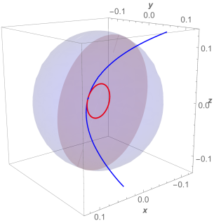
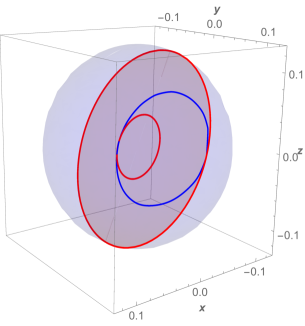
Figure 2: Plot of the trajectories of $\beta=1$ for the values $E=-1$ (left), $E=-6$ (right), ${\kappa}=-1$, $\ell=0.25$ and $\ell_{z}=0.1$.

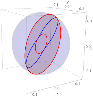
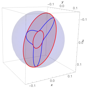
Figure 3: Plot of the trajectories of $\beta=2$ (left), $\beta=3$ (right) for the values $E=-6$, ${\kappa}=-1$, $\ell=0.25$ and $\ell_{z}=0.1$.

3.4 Algebra of the constants of motion for the Perlick system type I

As we have seen in the previous sections, we have obtained seven constants of motion for the three dimensional Perlick system: $H,H_{\theta\varphi},H_{\varphi},X^{\pm},Y^{\pm}$. Only five of these constants are independent, for example we can choose: $H,H_{\theta\varphi},H_{\varphi}$, $X^{+},Y^{+}$. Therefore, the Perlick system type I for a rational $\beta=m/n$ is a maximally superintegrable system. It turns out that, all the aforementioned seven constants are useful to express in a simple form the algebraic structure defined in terms of Poisson brackets:

$$\begin{array}[]{l}\{H,\cdot\}=0\,,\qquad\{H_{\theta\varphi},Y^{\pm}\}=0\,,\qquad\{H_{\theta\varphi},X^{\pm}\}=\pm 2\,i\,m\,\sqrt{H_{\theta\varphi}}\,X^{\pm},\\[8.61108pt] \{H_{\varphi},Y^{\pm}\}=\mp\,2\,i\,\sqrt{H_{\varphi}}Y^{\pm}\,,\qquad\{H_{\varphi},X^{\pm}\}=0\,,\qquad\{Y^{+},Y^{-}\}=2\,i\,\sqrt{H_{\varphi}}\left(H_{\theta\varphi}-2H_{\varphi}\right),\\[8.61108pt] \{X^{+},X^{-}\}=i\,m\,n\,(H_{\theta\varphi}-H_{\varphi})^{m}\,(H_{\xi}+\dfrac{1}{2}(\dfrac{1}{H_{\theta\varphi}}-{\kappa}\,H_{\theta\varphi}))^{n-1}({\kappa}\,\sqrt{H_{\theta\varphi}}+\dfrac{1}{H_{\theta\varphi}^{3/2}})\\[8.61108pt] \hskip 56.9055pt-2\,i\,m^{2}(H_{\theta\varphi}-H_{\varphi})^{m-1}\,(H_{\xi}+\dfrac{1}{2}(\dfrac{1}{H_{\theta\varphi}}-{\kappa}\,H_{\theta\varphi}))^{n}\,\sqrt{H_{\theta\varphi}},\\[8.61108pt] \{X^{\pm},Y^{\pm}\}=\mp\dfrac{i\,m}{\sqrt{H_{\theta\varphi}}+\sqrt{H_{\varphi}}}X^{\pm}Y^{\pm},\qquad\{X^{\pm},Y^{\mp}\}=\mp\dfrac{i\,m}{\sqrt{H_{\theta\varphi}}-\sqrt{H_{\varphi}}}X^{\pm}Y^{\mp}\,.\end{array}$$ (3.35)

In this way, we have found the algebra of the constants of motion for any two coprime integers $m$ and $n$ and any value of the constant ${\kappa}$. The corresponding polynomial algebras can be found as in [23].

The complex constants of motion $X^{\pm}$ and $Y^{\pm}$ allow to get real constants: $Y_{R}={\rm Re}(Y^{\pm}),Y_{I}={\rm Im}(Y^{\pm})$, $X_{R}={\rm Re}(X^{\pm}),X_{I}={\rm Im}(X^{\pm})$, which will close a real algebra. Besides, for $\beta=1,{\kappa}=0$, the complex constants of motion $X^{\pm}$ can be expressed in terms of the angular momentum ${\bf L}=(L_{x},L_{y},L_{z})$ and Runge-Lenz ${\boldsymbol{\cal A}}=({\cal A}_{x},{\cal A}_{y},{\cal A}_{z})$ vectors,

$$X^{\pm}={\rm Re}(X^{\pm})\pm i\,{\rm Im}(X^{\pm})=\dfrac{{\cal A}_{z}}{\sqrt{2}}\pm i\dfrac{({\bf L}\times{\boldsymbol{\cal A}})_{z}}{\sqrt{2}\,\ell}\,,$$ (3.36)

where

$${\boldsymbol{\cal A}}={\bf p}\times{\bf L}-\hat{\bf r}\,.$$ (3.37)

Here, we have used the expressions of ${\bf r},{\bf p},{\bf L}$ in spherical coordinates. Notice that in the context of the analysis of the Perlick system, a generalization of the Runge-Lenz vector has been proposed in ref. [5]. In the next section we will consider the motion in a plane corresponding to special case $\theta=\pi/2$.

4 Special case of the Perlick system type I

In this section, we will study the motion of the Perlick system type I in a plane, in this way we want to simplify the relevant constants of motion and the expression of the trajectories determined by such constants.

Let us take $\theta=\pi/2$; with this election the motion is limited to $x$-$y$ plane and the angular momentum along the $z$-axis is equal to the total angular momentum: ${\bf L}=(0,0,L_{z})$ $(\ell=\ell_{z})$. The corresponding Hamiltonian in the remaining $r,\varphi$ variables is

$$\widetilde{H}^{\pm}=\beta^{2}(1+K\,r^{2})\,\dfrac{p_{r}^{2}}{2}+\dfrac{{p_{\varphi}}^{2}}{2\,r^{2}}\pm\dfrac{1}{r}\,\sqrt{1+K\,r^{2}}\,.$$ (4.1)

Now, we have two trivial constants of motion: the total energy $E$ and $\ell_{z}$. Following the same procedure as in Sections 2, 3, with the change of the variables $(r,p_{r})$ by $(\xi,p_{\xi})$, we get the Hamiltonian

$$H(\xi,\theta,\varphi)=\beta^{2}\,\dfrac{p_{\xi}^{2}}{2}+\dfrac{{p_{\varphi}}^{2}}{2}\frac{1}{{\rm\ \!S}_{\kappa}^{2}(\xi)}-\frac{1}{{\rm\ \!T}_{\kappa}(\xi)}\,,$$ (4.2)

with the same range of the variable $\xi$ as specified in Section 2. In this case the effective Hamiltonian $H_{\xi}$ is given by

$$H_{\xi}=\beta^{2}\,\dfrac{p_{\xi}^{2}}{2}+\dfrac{{\ell_{z}}^{2}}{2}\frac{1}{{\rm\ \!S}_{\kappa}^{2}(\xi)}-\frac{1}{{\rm\ \!T}_{\kappa}(\xi)}=\beta^{2}\,\dfrac{p_{\xi}^{2}}{2}+V_{\rm eff}({\xi})\,.$$ (4.3)

It is easy to find two additional constants of motion $Z^{\pm}$ for the Hamiltonian (4.2):

$$\{H,Z^{\pm}\}=0\,,\qquad Z^{\pm}=(D^{\pm})^{m}(B^{\mp})^{n}\,,$$ (4.4)

where

$$B^{\pm}=\frac{1}{\sqrt{2}}\,\left(\mp\,i\,{\beta}\,{p_{\xi}}+\frac{\ell_{z}}{{\rm\ \!T}_{\kappa}{(\xi)}}-\dfrac{1}{\ell_{z}}\right)\,,\qquad D^{\pm}=\sqrt{H_{\varphi}}\,e^{\mp i\,\varphi}\,,$$ (4.5)

and

$$H_{\xi}=B^{+}B^{-}+\lambda_{\xi}\,,\qquad\lambda_{\xi}=-\dfrac{1}{2}\left(\dfrac{1}{\ell_{z}^{2}}-{\kappa}\,\ell_{z}^{2}\right)\,,$$ (4.6)

$$H_{\varphi}=p_{\varphi}^{2}=D^{+}D^{-}\,.$$ (4.7)

These constants of motion $Z^{\pm}$ have complex values denoted by

$$Z^{\pm}=q_{z}\,e^{\pm i\,\varphi_{z}}\,,$$ (4.8)

where $-\pi\leq\varphi_{z}<\pi$ and $0\leq q_{z}<\infty$. The modulus $q_{z}$ has a value determined by the other constants of motion $E$ and $\ell_{z}$,

$$q_{z}=|Z^{\pm}|=\ell_{z}^{m}\left(E+\dfrac{1}{2}\,\left(\dfrac{1}{\ell_{z}^{2}}-{\kappa}\,\ell_{z}^{2}\right)\right)^{n/2}\,.$$ (4.9)

The functions $B^{\pm}$ and $D^{\pm}$ can be written as

$$\begin{array}[]{l}B^{\pm}(\xi,p_{\xi})=\left(E+\dfrac{1}{2}\,\left(\dfrac{1}{\ell_{z}^{2}}-{\kappa}\,\ell_{z}^{2}\right)\right)^{1/2}e^{\pm i\,b(\xi,p_{\xi})}\,,\\[10.76385pt] D^{\pm}(\varphi,p_{\varphi})=\ell_{z}\,e^{\pm i\,d(\varphi,p_{\varphi})}\,,\end{array}$$ (4.10)

where $b(\xi,p_{\xi})$ and $d(\varphi,p_{\varphi})$ are the corresponding real phase functions. When the energy $E$ satisfies the restriction (3.5), the bounded motion of the variables $(\xi,p_{\xi})$ is periodic. Besides, the motion of the variables $(\varphi,p_{\varphi})$ is also periodic, due to the angular character of $\varphi$. Then, substituting in (4.8) we get

$$m\,d(\varphi,p_{\varphi})-n\,b(\xi,p_{\xi})=\varphi_{\rm z},\qquad\xi_{1}\leq\xi\leq\xi_{2}\,,\quad-\pi\leq\varphi<\pi\,.$$ (4.11)

Hence, after differentiating with respect to the time we obtain the relation between the frequencies of the two variables:

$$m\,\omega_{\varphi}-n\,\omega_{\xi}=0\,.$$ (4.12)

Let us write the equation of the constant of motion $Z^{\pm}$,

$$(\ell_{z}\,e^{\mp i\,\varphi})^{m}\,(\mp i\,\dfrac{\beta}{\sqrt{2}}\,{p_{\xi}}+\dfrac{\ell_{z}}{\sqrt{2}}\dfrac{1}{{\rm\ \!T}_{\kappa}(\xi)}-\dfrac{1}{\ell_{z}\,\sqrt{2}})^{n}=q_{z}\,e^{\pm i\,\varphi_{z}}\,.$$ (4.13)

Taking the real and imaginary parts of this equality, we get two equations

$$\dfrac{\ell_{z}}{\sqrt{2}}\frac{1}{{\rm\ \!T}_{\kappa}(\xi)}-\dfrac{1}{\ell_{z}\,\sqrt{2}}=\left(\dfrac{q_{z}}{\ell_{z}^{m}}\right)^{1/n}\cos{\left(\frac{1}{n}\varphi_{z}+\frac{m}{n}\varphi\right)}\,,$$ (4.14)

$$-\dfrac{\beta}{\sqrt{2}}\,{p_{\xi}}=\left(\dfrac{q_{z}}{\ell_{z}^{m}}\right)^{1/n}\sin{\left(\frac{1}{n}\varphi_{z}+\frac{m}{n}\varphi\right)}\,.$$ (4.15)

From (4.14), we obtain the relation between $\xi$ and $\varphi$ along the trajectories [5]:

$$\cos{\left(\frac{1}{n}\varphi_{z}+\dfrac{m}{n}\varphi\right)}=\frac{\dfrac{\ell_{z}^{2}}{{\rm\ \!T}_{\kappa}(\xi)}-1}{\sqrt{2\,E\,\ell_{z}^{2}+1-{\kappa}\,\ell_{z}^{4}}}\,.$$ (4.16)

Relation (4.16) becomes a well known conic section equation for the values ${\kappa}=0$ , $\beta=m/n=1$ and $\varphi_{z}=0$:

$$\frac{\alpha}{\xi}=1+\varepsilon\,\cos{\varphi}\,,$$ (4.17)

where $\varepsilon^{2}=2\,E\,\ell_{z}^{2}+1$ (eccentricity) and $\alpha=\ell_{z}^{2}$ (semi-latus rectum) [35]. In this case, the problem is reduced to the Kepler-Coulomb system in the Euclidean plane. If ${\kappa}=-1$ (${\kappa}=1$) and $\beta=1$, then we get the conic section equation in the hyperboloid (sphere) [13]:

$${\kappa}=-1\,,\quad{(\rm Hyperbolic)}\qquad\dfrac{\alpha}{\tanh{\xi}}=1+\sqrt{\varepsilon^{2}+\alpha^{2}}\,\cos{\varphi}\,,$$ (4.18)

$${\kappa}=1\,,\quad{(\rm Spherical)}\qquad\dfrac{\alpha}{\tan{\xi}}=1+\sqrt{\varepsilon^{2}-\alpha^{2}}\,\cos{\varphi}\,.$$ (4.19)

So, we may say that the equation (4.16) can be considered as a generalized conic section equation. Taking into account the relation (4.18) for ${\kappa}=-1$ and the relation (4.19) for ${\kappa}=1$ different examples of trajectories $(\xi\,\cos\varphi,\xi\,\sin\varphi)$, where $(\xi,\varphi)$ are polar coordinates, are plotted in Figs. 4-7. In these figures there are represented bounded and unbounded trajectories, according to the values of the energy $E$. In the case of bounded motion, due to the above relation of the frequencies (4.12) the motion must be periodic and the trajectories are closed.

In the special case where ${\kappa}=0$ and $\beta=m/n=1$, the constants of motion $Z^{\pm}$ can also be expressed in terms of the Runge-Lenz vector ${\boldsymbol{\cal A}}=({\cal A}_{x},{\cal A}_{y},0)$,

$$Z^{\pm}={\rm Re}(Z^{\pm})\pm i\,{\rm Im}(Z^{\pm})=\dfrac{{\cal A}_{x}}{\sqrt{2}}\mp i\dfrac{{\cal A}_{y}}{\sqrt{2}}\,.$$ (4.20)

For the other cases (${\kappa}=\pm 1$), the constants of motion $Z^{\pm}$ can be written in terms of a type of generalized Runge-Lenz vector [5]. Note that, the constants $H,H_{\varphi},Z^{\pm}$ close a similar algebra as in the general case.

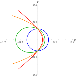
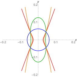
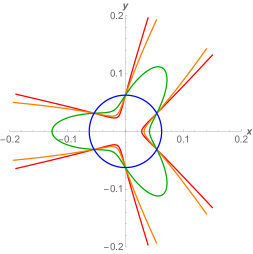
Figure 4: Plot of the trajectories of $\beta=1$ (left), $\beta=2$ (center), $\beta=3$ (right) for the values $E=-8.03$ (minimum energy of the potential), $E=-6,E=-1,E=4$. For $\beta=1$, respectively. Here we have chosen ${\kappa}=-1$, $\ell=0.25$ and $\ell_{z}=0.1$.

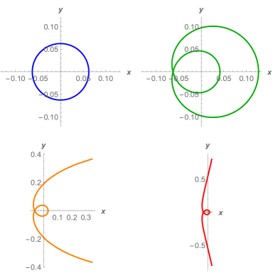
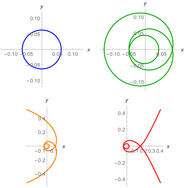
Figure 5: Plot of the trajectories of $\beta=1/2$ (left), $\beta=1/3$ (right) for the values $E=-8.03$ (minimum energy of the potential), $E=-6,E=-1,E=4$, corresponding to circular, elliptic, parabolic and hyperbolic orbits, respectively. Here we have chosen ${\kappa}=-1$, $\ell=0.25$ and $\ell_{z}=0.1$.

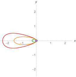
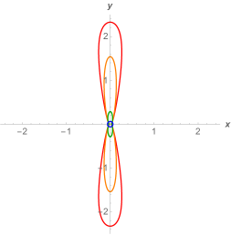
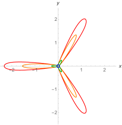
Figure 6: Plot of the trajectories of $\beta=1$ (left), $\beta=2$ (center), $\beta=3$ (right) for the values $E=-7.96875$ (minimum energy of the potential), $E=-3,E=0,E=1$. Here we have chosen ${\kappa}=1$, $\ell_{z}=0.25$.

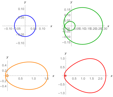
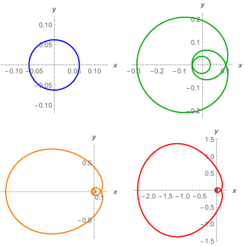
Figure 7: Plot of the trajectories of $\beta=1/2$ (left), $\beta=1/3$ (right) for the values $E=-7.96875$ (minimum energy of the potential), $E=-3,E=0,E=1$. Here we have chosen ${\kappa}=1$, $\ell_{z}=0.25$.

5 Conclusions and remarks

In this paper, we have started an algebraic approach to the study of Perlick’s systems, the family of maximally superintegrable systems discovered in 1992, that represent the most general extension of the classical Bertrand systems to curved (though conformally flat) N-dimensional (Riemannian) manifolds. We would summarize our main new findings as follows. On one hand, we have given a thorough description of the algebraic and geometrical properties of the classical Perlick system of type I by means of the factorization approach: we have identified both the shift and the ladder functions for the radial as well as for the angular Hamiltonian. Henceforth, we have been able to identify the full set of constants of motion and their related Poisson algebra, and unveiled the intimate connection with the geometric features of the orbits provided by superintegrability. On the other hand, we have been able to single out the role played by the two parameters that characterize the system: the real parameter $K$, entering both in the metrics and in the potential, is related with the compact or non-compact nature of the manifold where the motion takes place; the rational parameter $\beta$, which does not appear in the potential, is in turn responsible for what we would call “the complexity” of the trajectories, namely their winding number. These features emerge in a perspicuous manner from the graphic representations of the (effective) potential as well as of the orbits, reported in a number of figures for different values of $K$ and $\beta$.

The further steps to be accomplished are clear. (i) We have to see how our construction goes over to the quantum setting, and (ii) we have to perform a similar construction for the full Perlick family II. Work is actually in progress in both directions, and promising preliminary results have been already obtained by the authors and their collaborators.

References

- [1]
- [2] V. Perlick, Bertrand spacetimes, Class. Quantum Grav. 9 (1992) 1009-1021.
- [3] A. Ballesteros, A. Enciso, F.J. Herranz and O. Ragnisco, A maximally superintegrable system on an n-dimensional space of nonconstant curvature, Phys. D 237 (2008) 505-509.
- [4] A. Ballesteros, A. Enciso and F.J. Herranz and O. Ragnisco, Bertrand spacetimes as Kepler/oscillator potentials, Class. Quantum Grav. 25 (2008) 165005.
- [5] A. Ballesteros, A. Enciso and F.J. Herranz and O. Ragnisco, Hamiltonian systems admitting a Runge-Lenz vector and an optimal extension of Bertrand’s theorem to curved manifolds, Comm. Math. Phys. 290 (2009) 1033-1049.
- [6] A. Ballesteros, A. Enciso, F.J. Herranz and O. Ragnisco, Superintegrability on N-dimensional curved spaces: central potentials, centrifugal terms and monopoles, Ann. Phys. 324 (2009) 1219-1233.
- [7] A. Ballesteros, A. Enciso, F.J. Herranz, O. Ragnisco and D. Riglioni, New superintegrable models with position-dependent mass from Bertrand’s theorem on curved spaces, J. Phys.: Conf. Ser. 284 (2011) 012011.
- [8] A. Ballesteros, A. Enciso, F.J. Herranz, O. Ragnisco and D. Riglioni, A new exactly solvable quantum model in N dimensions, Phys. Lett. A 375 (2011) 1431-1435.
- [9] A. Ballesteros, A. Enciso, F.J. Herranz, O.Ragnisco and D. Riglioni, Quantum mechanics on spaces of nonconstant curvature: the oscillator problem and superintegrability, Ann. Phys. 326 (2011) 2053-2073.
- [10] D. Latini, A. Ballesteros, A. Enciso, F.J. Herranz, O. Ragnisco and D. Riglioni, The classical Darboux III oscillator: factorization, Spectrum Generating Algebra and solution to the equations of motion, J. Phys.: Conf. Ser. 670 (2016) 012031.
- [11] T. Iwai and N. Katayama, Multifold Kepler systems - dynamical systems all of whose bounded trajectories are closed, J. Math. Phys. 36 (1995) 1790-1811.
- [12] J. Bertrand, Théorème relatif au mouvement d’un point attire vers un centre fixe, C. R. Acad. Sci. Paris 77 (1873) 849-853.
- [13] J.F. Cariñena, M.F. Rañada and M. Santander, Central potentials on spaces of constant curvature: The Kepler problem on the two-dimensional sphere and the hyperbolic plane, J. Math. Phys. 46 (2005) 052702.
- [14] E.G. Kalnins, W. Miller Jr. and G.S. Pogosyan, Coulomb-oscillator duality in spaces of constant curvature, J. Math. Phys. 41 (2000) 2629-2657.
- [15] E.G. Kalnins and W. Miller Jr., Structure theory for extended Kepler-Coulomb 3D classical superintegrable systems, SIGMA 8 (2012) 034.
- [16] S. Wojciechowski, Superintegrability of the Calogero-Moser system, Phys. Lett. 95A (1983) 279-281.
- [17] N.W. Evans, Superintegrability in classical mechanics, Phys. Rev. A 41 (1990) 5666-5676.
- [18] W. Miller Jr., S. Post and P. Winternitz, Classical and quantum superintegrability with applications, J. Phys. A: Math. Theor. 46 (2013) 423001.
- [19] Ş. Kuru and J. Negro, Factorizations of one-dimensional classical systems, Ann. Phys. 323 (2008) 413-431.
- [20] V. Hussin and I. Marquette, Generalized Heisenberg algebras, SUSYQM and degeneracies: infinite well and Morse potential, SIGMA 7 (2011) 024.
- [21] Ş. Kuru and J. Negro, ‘Spectrum generating algebras’ of classical systems: the Kepler-Coulomb potential, J. Phys.: Conf. Ser. 343 (2012) 012063.
- [22] E. Celeghini, Ş. Kuru, J. Negro and M.A. del Olmo, A unified approach to quantum and classical TTW systems based on factorizations, Ann. Phys. 332 (2013) 27-37.
- [23] J.A. Calzada, Ş. Kuru, J. Negro, Superintegrable Lissajous systems on the sphere, Eur. Phys. J. Plus 129 (2014) 164.
- [24] A. Ballesteros, F.J. Herranz, Ş. Kuru and J. Negro, The anisotropic oscillator on curved spaces: A new exactly solvable model, Ann. Phys. 373 (2016) 399-423.
- [25] A. Ballesteros, F.J. Herranz, Ş. Kuru and J. Negro, Factorization approach to superintegrable systems: formalism and applications, Phys. At. Nucl. 80 (2017) 389-396.
- [26] D. Latini and O. Ragnisco, The classical Taub-Nut System: factorization, spectrum generating algebra and solution to the equations of motion, J. Phys. A: Math. Theor. 48 (2015) 175201.
- [27] F. Tremblay, A.V. Turbiner and P. Winternitz, Periodic orbits for an infinite family of classical superintegrable systems, J. Phys. A: Math. Theor. 43 (2010) 015202.
- [28] T. Hakobyan, O. Lechtenfeld, A. Nersessian, A. Saghatelian and V. Yeghikyana, Integrable generalizations of oscillator and Coulomb systems via action-angle variables, Phys. Lett. A 376 (2012) 679-686.
- [29] D. Riglioni, Classical and quantum higher order superintegrable systems from coalgebra symmetry, J. Phys. A: Math. Theor. 46 (2013) 265207.
- [30] S. Post and D. Riglioni, Quantum integrals from coalgebra structure, J. Phys. A: Math. Theor. 48 (2015) 075205.
- [31] I. Marquette and P. Winternitz, Polynomial Poisson algebras for classical superintegrable systems with a third-order integral of motion, J. Math. Phys. 48 (2007) 012902.
- [32] I. Marquette, Quartic Poisson algebras and quartic associative algebras and realizations as deformed oscillator algebras, J. Math. Phys. 54 (2013) 071702.
- [33] C. Quesne and V.M. Tkachuk, Deformed algebras, position dependent effective masses and curved spaces: an exactly solvable Coulomb problem, J. Phys. A: Math. Gen. 37 (2004) 4267-4281.
- [34] A. Ballesteros, I. Gutiérrez-Sagredo and P. Naranjo, On Hamiltonians with position-dependent mass from Kaluza-Klein compactifications, Phys. Lett. A 381 (2017) 701-706.
- [35] H. Goldstein, C.P. Poole and J.L. Safko, Classical Mechanics (3rd Edition) (Addison-Wesley, New York, 2001).
- [36] F.J. Herranz and M. Santander, Conformal symmetries of spacetimes, J. Phys. A: Math. Gen. 35 (2002) 6601-6618.
- [37] M.F. Rañada and M. Santander, Superintegrable systems on the two dimensional sphere and the hypebolic plane , J. Math. Phys. 40 (1999) 5026-5057.