Voronoi chords in flat cosmology

Abstract

In this paper we present formulae for chord length distribution in the framework of Poissonian Voronoi Tessellation (PVT) and non Poissonian Voronoi Tessellation (NPVT). The introduction of the scale parameter in the obtained distributions allows us to model the chord for cosmic voids. A graphical comparison between cosmic voids visible on two catalogs of galaxies, 2dFGRS and VIPERS, and theoretical random chords is reported.

1 Introduction

A first study on the random 3D fragmentation by [1] was done in the framework of Voronoi Diagrams. In the above paper the Kiang’s conjecture was introduced: ”The normalized probability density function for volumes in Poissonian Voronoi Tessellation follows a normalized gamma distribution with shape parameter $c$ equal to six”. A subsequent large-scale computer simulation on Poissonian Voronoi Tessellation (PVT), see [2], fixed in $c=5$ the shape parameter of the normalized gamma distribution, in the following Kiang’s function The shape parameter $c$ plays an important role in the determination of the probability density function (PDF) which model the Poissonian and non Poissonian Voronoi Tessellation (NPVT) chord, see [3, 4]. The 3D tessellation is built in the framework of the Euclidean distance conversely in astronomy the observable parameter is the redshift $z$. In cosmology a key target is to deduce the luminosity distance as a function of the redshift, see as an example [5] where different models were analyzed. The inverse problem, i.e., the redshift as function of the luminosity distance, is poorly known and this fact has stopped the application of the Voronoi Diagrams to cosmology. The enormous progresses in observational cosmology allows to model the radius of cosmic voids, see [6, 7]. A statistical analysis of these catalogs allows the determination of the shape parameter $c$ of the Kiang’s function. This paper explores in Section 2 the fundamentals of chord for spheres and reviews the existing knowledge for volumes in PVT and NPVT. In section 3 a PDF for chord in PVT and NPVT is investigated. The luminosity distance as function of the redshift in flat cosmology and the corresponding inverse function is derived in Section 4. Section 5 reports a comparison between real voids of galaxies and theoretical random cosmic chord.

2 The basic formulae

This Section reviews the basic formulae for chords of spheres and the distribution in volumes for PVT and NPVT.

2.1 The chord

The average length, $<l>$, of all chords of spheres having the same radius $R$

$$<l>=\frac{4}{3}R\quad,$$ (1)

see more details in [3].

Given a probability density function (PDF) for the diameter of the voids, $F(x)$, where $x$ indicates the diameter. The probability, $G(x)dx$, that a sphere having diameter between $x$ and $x+dx$ intersects a random line is proportional to their cross section

$$G(x)dx=\frac{\frac{\pi}{4}x^{2}F(x)dx}{\int_{0}^{\infty}\frac{\pi}{4}x^{2}F(x)dx}=\frac{x^{2}F(x)dx}{<x^{2}>}\quad.$$ (2)

Given a line which intersects a sphere of diameter $x$, the probability that the distance from the center lies in the range $r,r+dr$ is

$$p(r)=\frac{2\pi rdr}{\frac{\pi}{4}x^{2}}\quad,$$ (3)

and the chord length is

$$l=\sqrt{x^{2}-4r^{2}}\quad.$$ (4)

The probability that spheres in the range $(x,x+dx)$ are intersected to produce chords with lengths in the range $(l,l+dl)$ is

$$G(x)\,dx\frac{2l\,dl}{x^{2}}=\frac{2l\,dl}{<x^{2}>}F(x)dx\quad.$$ (5)

The probability of having a chord with length between $(l,l+dl)$ is

$$g(l)=\frac{2l}{<x^{2}>}\int_{l}^{\infty}F(x)dx\quad.$$ (6)

This integral will be called fundamental and the previous demonstration follows [8, 3].

2.2 Voronoi Diagrams

The Voronoi tessellation is the partition of space for a given seeds pattern and the result of the partition depends completely on the type of given pattern ”random”, Poisson-Voronoi tessellations (PVT), or ”non-random”, non Poisson-Voronoi tessellations (NPVT). The reduced volumes of Voronoi cells generated with random seeds can be fitted by the Kiang function

$$p(x;c)=\frac{c^{c}}{\Gamma(c)}x^{c-1}\exp(-cx),$$ (7)

see [1], which has variance

$$\sigma^{2}=\frac{1}{c}.$$ (8)

It has shown that good approximations for volume distributions of PVT cells can be obtained by setting $c=5$ [2, 4]. The case of more regular partition of the space is produced by the Sobol seeds which produce a distribution in volumes with $c\approx 16$. Conversely the introduction of seeds generated on a adjustable Cartesian grid (ACG) allows to cover the interval $c\in(2-16)$ in a continuous way, see [4]. Figure 1 reports three cases of volumes for the Voronoi Diagrams from which is clear the transition from order to disorder as function of decreasing c.

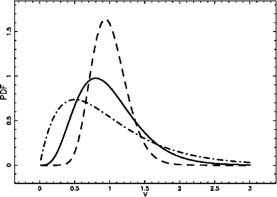
Figure 1: Reduced volume distribution when c=5 (full line), c=16 (dashed line) and c=2 (dot-dash-dot-dash line).

3 The generalized chord

We start by approximating the reduced volumes of the Voronoi tessellation by a Kiang function, therefore the distribution in diameters, $y$, is

$$F(y)=\frac{c\left(\frac{1}{6}\,c\pi\,{{\it y}}^{3}\right)^{c-1}{{\rm e}^{-\frac{1}{6}\,c\pi\,{{\it y}}^{3}}}\pi\,{{\it y}}^{2}}{2\,\Gamma\left(c\right)}\quad,$$ (9)

where

$$\mathop{\Gamma\/}\nolimits\!\left(x\right)=\int_{0}^{\infty}e^{{-t}}t^{{x-1}}dt\quad,$$ (10)

is the gamma function. We insert in the fundamental Equation (6) for the chord length the generalized PDF for the diameters. The resulting integral is

$$g(l;c)=\frac{-{\pi}^{2/3}\sqrt[3]{6}l\left({6}^{-c}{c}^{c}{\pi}^{c}{l}^{3\,c}{{\rm e}^{-1/6\,c\pi\,{l}^{3}}}-\Gamma\left(1+c,1/6\,c\pi\,{l}^{3}\right)\right)}{3\,\sqrt[3]{c}\Gamma\left(2/3+c\right)}\quad,$$ (11)

where

$$\mathop{\Gamma\/}\nolimits\!\left(a,z\right)=\int_{z}^{\infty}t^{{a-1}}e^{{-t}}dt,$$ (12)

is the upper incomplete gamma function, see [9, 10].

Figure 2 reports three cases of $g(l;c)$ as function of $c$.

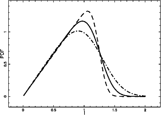
Figure 2: Chord PDF for Voronoi Diagrams, g(l;c), when c=5 (full line), c=16 (dashed line) and c=2 (dot-dash-dot-dash line)

We have approximated the volumes of the Voronoi diagrams by spheres and the length of the chord which touches only in one point the sphere is zero, conversely a chord which lies on a irregular face of the Voronoi’s polyhedron has a finite length. In order to solve this inconvenient a shift should be introduced. A new variable $z$ has been defined by a shift of $l$: $z=l-a$, so that

$$g_{s}(z;c,a)=g(z+a;c,a)\quad,$$ (13)

where $a$ is the shift parameter and $g_{s}(z;c,a)$ is the shifted PDF for Voronoi’s chord. Next, to obtain a reduced variable, average value equal one or an astrophysical variable, a scale change has been applied ,$u=bz$, resulting in scaled PDF for chords

$$g_{b}(u;c,a,b)=\frac{g_{s}(\frac{u}{b};c,a)}{b}\quad.$$ (14)

As an example the PVT PDF for chords, $c=5$, can be obtained inserting $a=0.4068$ and $b$ =1.9626 and is

$$g_{b}(u;5,0.4068,1.9626)=(0.3690+0.0002321\,{u}^{13}+0.002410\,{u}^{12}+0.01155\,{u}^{11}+0.03649\,{u}^{10}$$

$$+0.08890\,{u}^{9}+0.1739\,{u}^{8}+0.2903\,{u}^{7}+0.4413\,{u}^{6}+0.5798\,{u}^{5}+0.7160\,{u}^{4}$$

$$+0.8327\,{u}^{3}+0.6931\,{u}^{2}+0.7065\,u){{\rm e}^{-0.3463\,(u+0.7985)^{3}}}\quad.$$ (15)

The above PDF in the interval $u\in(0,3.2)$ is normalized to one and has average value one. The distribution function (DF) of this PDF does not exists but the best minimax rational approximation of degree (5, 2) allows to find the following approximate distribution function, $DF_{5}$,

$$DF_{5}(x)=\frac{0.4446+0.1266\,x-0.4449\,{x}^{2}+0.1910\,{x}^{3}-0.02560\,{x}^{4}+0.0004040\,{x}^{5}}{1.447-1.462\,x+0.4596\,{x}^{2}}\quad.$$ (16)

Figure 3 reports a comparison of the previous approximate DF, as a dashed line with the tabulated result as deduced from Table 5.7.4 in [11] when the average value of both PDFs is one.

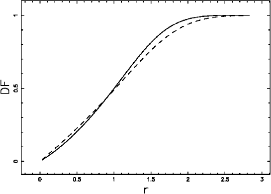
Figure 3: The full line represents the tabulated chord DF in the case of PVT, the dashed line is our chord approximate $DF_{5}$.

4 Flat cosmologies with cosmological constant

As eqn.(2.1) in [12] the luminosity distance $dl$ is

$$d_{L}(z;c,H_{0},\Omega_{\rm M})=\frac{c}{H_{0}}(1+z)\int_{\frac{1}{1+z}}^{1}\frac{da}{\sqrt{\Omega_{\rm M}a+(1-\Omega_{\rm M})a^{4}}}\quad,$$ (17)

where $H_{0}$ is the Hubble constant expressed in $\mathrm{km\,s^{-1}\,Mpc^{-1}}$, $c$ is the light velocity expressed in $\mathrm{km\,s^{-1}}$, $z$ is the redshift, $a$ is the scale-factor and $\Omega_{\rm M}$ is

$$\Omega_{\rm M}=\frac{8\pi\,G\,\rho_{0}}{3\,H_{0}^{2}}\quad,$$ (18)

where $G$ is the Newtonian gravitational constant and $\rho_{0}$ is the mass density at the present time. The above integral does not have an analytical simple formula but the Padé approximation of degree $m,n$ about the point $a$=1 of the integrand allows to solve in an approximate way the integral.

We report the Padé approximate integral of the luminosity distance $d_{L,2,2}$, in the case of $m$=2 and $n$=2 when $H_{0}=100\mathrm{km\,s^{-1}\,Mpc^{-1}}$ and $\Omega_{\rm M}=0.3$ as in [7]

$$d_{L,2,2}(z)=\Re\bigg{(}2997.924\,(1+z)(-0.0953787\,(1+z)^{-1}+1.04035-0.55174\,i+$$

$$0.175624\,\ln(-624.128\,(1+z)^{-2}+92.2245\,(1+z)^{-1}-284.222)$$

$$-2.248466\,\arctan(1.490823\,(1+z)^{-1}-0.110146))\bigg{)}\quad.$$ (19)

In the above complex analytical solution we have a real part denoted by $\Re$ and a negligible imaginary part. As an example the above real part is 23977.70565 when $z=4$ and the imaginary part is $0.5546\,10^{-4}$.

In the above formula $d_{L,2,2}$ is function, $f$, of $z$

$$d_{L,2,2}=f(z)\quad.$$ (20)

The inverse function $f^{-1}$ is

$$z=f^{-1}(d_{L,2,2})$$ (21)

but eqn. (19) is not invertible for $z$.

In order to have an inverse function we apply the best minimax rational approximation of degree (m, n) to eqn.(19) over the interval $z\,\in(0,4)$. In the case of $m$=2 and $n$=2 the minimax rational expression for the luminosity distance, $d_{L,m,2,2}$, is

$$d_{L,m,2,2}=\frac{1.792+1292.747\,z+2020.755\,{z}^{2}}{0.4463702+0.2686967\,z+0.002703757\,{z}^{2}}\quad.$$ (22)

The inverse function exists and is

$$z=\frac{N(d_{L})}{D(d_{L})}\quad,$$ (23)

where

$$N=-6.71741\,10^{9}\,{\it d_{L}}+3.231869\,10^{13}$$

$$-\sqrt{{4.210652\times 10^{19}}\,{{\it d_{L}}}^{2}+{1.820828\times 10^{24}}\,{\it d_{L}}+{1.035444754\times 10^{27}}}$$

and

$$D=1.35187\,10^{8}\,{\it d_{L}}-1.010377933\,10^{14}\quad.$$

In the framework of a numerical approximation for the inverse function

$$f(f^{-1}(x_{1}))=x2\quad,$$ (24)

with $x_{1}\approx x_{2}$, we introduce the percentage error, $\delta$, of the inversion formula (23)

$$\delta=\frac{\big{|}x_{1}-x_{2}\big{|}}{X_{1}}\,100\quad.$$ (25)

In our case when $x_{1}=1200\,Mpc$ $f(f^{-1}(1200\,Mpc))=1203.4\,Mpc$ which means $\delta=0.027\%$.

5 Astrophysical Applications

This section processes two astronomical catalogs for cosmic voids, deduces PDF and DF for astrophysical chord, introduces the cosmic chord and randomly generates chords on two catalogs of galaxies.

5.1 The catalogs of voids

A first catalog of cosmic voids can be found in [6] where the effective radius of the voids has been derived. The main results, the averaged radius of the voids and the value of $c$ for the reduced volumes of spheres, are

$$R=18.23h^{-1}\,Mpc\quad;\quad c=1.458\quad Pam\,et\,al.\,2012\quad,$$ (26)

we call it the non Poissonian case. A second catalog is that of radii larger than 10h-1Mpc up to redshift $0.12\,h^{-1}Mpc$ in (SDSS-DR7), see [7]. In this case the average radius and $c$ are

$$R=11.85h^{-1}\,Mpc\quad;\quad c=4.763\quad Varela\,et\,al.\,2012\quad,$$ (27)

we call it the nearly Poissonian case, being the Poissonian case $c$=5.

5.2 Astrophysical chords

An astrophysical version for the PDF of chords can be obtained inserting in eqn.14 the appropriate scale, $b$, and the shape parameters, $c$, see Table 1

Table 1: Parameters of the astrophysical chords.

Case	a	b (Mpc)	c	$<l>$ (Mpc)
Nearly  Poissonian	.402	30.7664	4.763	15.799
Non Poissonian	.345	40.2374	1.458	24.306

The PDF which models the chord for cosmic voids in the nearly Poissonian case is

$$g_{b,nearly}(x)=-0.00033275\,\sqrt[3]{6}(0.032502\,x+0.40268)\bigg{(}77.24\,(0.032502\,x+0.40268)^{14.28}$$

$${{\rm e}^{-2.49233\,(0.0325\,x+0.40268)^{3}}}-\Gamma(5.76,2.49233\,(0.032502\,x+0.40268)^{3})\bigg{)}\quad nearly~{}Poissonian\quad,$$ (28)

and in the non Poissonian case is

$$g_{b,non}(x)=-0.0162275\,\sqrt[3]{6}(0.0248524\,x+0.345018)\bigg{(}0.670705\,(0.0248524\,x+0.345018)^{4.35}$$

$${{\rm e}^{-0.759218\,(0.0248524\,x+0.345)^{3}}}-\Gamma(2.45,0.759218\,(0.024852\,x+0.345)^{3})\bigg{)}\quad non~{}Poissonian\quad.$$ (29)

The two previous PDFs cannot be integrated and therefore the analytical DFs do not exist. We therefore first deduce two approximate PDFs trough the best minimax rational approximation of degree (5, 2). The integration of the two approximate PDFs gives

$$DF_{nearly}(x)=-0.0000036854\,{x}^{3}+0.00047203\,{x}^{2}-0.0030029\,x$$

$$-0.30287\,\ln\left(593907229\,{x}^{2}-29656460050\,x+468265974500\right)$$

$$+0.19796\,\arctan\left(0.077829\,x-1.9431\right)+8.3557$$ (30)

in the nearly Poissonian case and

$$DF_{non}(x)=-0.0000013322\,{x}^{3}+0.00033491\,{x}^{2}-0.014562\,x$$

$$-0.63054\,\ln\left(1142509457\,{x}^{2}-77777418420\,x+2468943718000\right)$$

$$+0.52222\,\arctan\left(0.031584\,x-1.0750\right)+18.421$$ (31)

in the non Poissonian case.

The random generation of astrophysical chords can be implemented by solving in $x$ the following non linear equation in the nearly Poissonian case

$$R=DF_{nearly}(x)\quad,$$ (32)

where $R$ is the unit rectangular variate.

The non linear equation to be solved in the non Poissonian case is

$$R=DF_{non}(x)\quad.$$ (33)

5.3 The cosmic chord

In the previous subsection we derived a couple of non linear equations for the astrophysical chords, we now outline an algorithm for the cosmic environment. We generated $n$ random chords in Mpc units solving one of the two non linear equations, (30) or (31). The random chords, denoted by $l_{j}$, are

$$l_{1},l_{2}\dots l_{n}\quad.$$ (34)

We assume the additivity of the luminosity distance, $d_{L,j}$, and therefore

$$d_{L,1}=l_{1}\quad d_{L,2}=l_{1}+l_{2}\quad\dots d_{L,n}=D_{l,n-1}+l_{n}\quad.$$ (35)

The conversion of the luminosity distance to the redshift is made trough formula (23)

$$z_{1}=\frac{N(d_{L,1})}{D(d_{L,1})}\quad z_{2}=\frac{N(d_{L,2})}{D(d_{L,2})}\quad\dots\quad z_{n}=\frac{N(d_{L,n})}{D(d_{L,n})}\quad.$$ (36)

A typical sequence is reported in Table 2.

Table 2: Ten random non Poissonian chords, $l$, luminosity distance, $d_{L}$, and corresponding redshift in flat cosmology.

l	$d_{L}$	z
38.96	38.96	0.0119
23.53	62.49	0.0198
18.57	81.06	0.0260
46.50	127.57	0.0411
12.06	139.63	0.0450
39.24	178.87	0.0574
47.43	226.29	0.0720
32.51	258.81	0.0819
14.25	273.06	0.0862
21.64	294.70	0.0926

A first interesting quantity to be evaluated is the number of chords, $N$, that cover a given interval in redshift, as an example (0,1), which is

$$N=188,\quad non~{}Poissonian~{}case\quad;\qquad N=271,\quad nearly~{}Poissonian~{}case.$$ (37)

Figure 4 reports the value reached in redshift for rising number of chords.

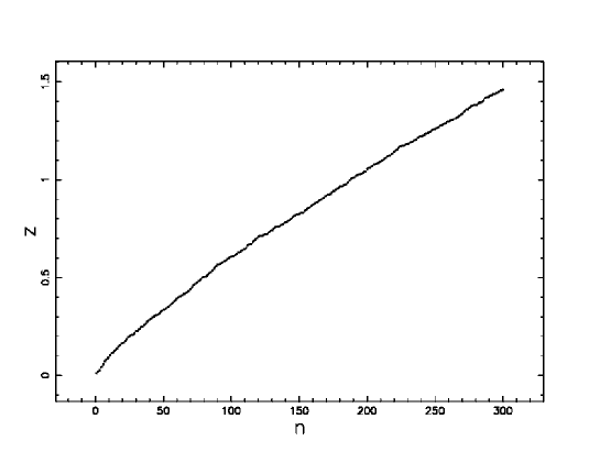
Figure 4: Value of redshift as function of the number of chords in the non Poissonian case.

5.4 The catalog of galaxies

A first catalog of galaxies is the two-degree Field Galaxy Redshift Survey, in the following 2dFGRS, see [13], in the interval $z\in(0.001,0.1)$ : two strips of the 2dFGRS are shown in Figure 5.

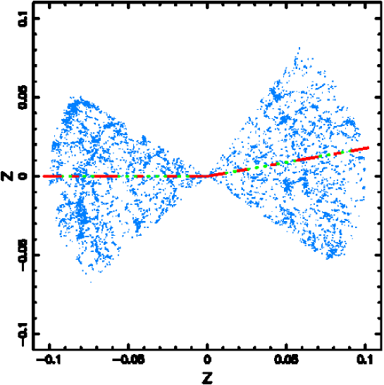
Figure 5: Cone-diagram of the galaxies in the 2dFGRS with $z$ $\in$ (0,0.1). This plot contains 10234 galaxies (blue color). Two sequence of chords in the non Poissonian case are reported, the first chord is red (full line), the second chord is green (dotted line).

A second catalog of galaxies is VIMOS Public Extragalactic Survey, in the following VIPERS, see [14]. We selected the W1 field when $z$ $\in$ (0.5,0.6), see Figure 6.

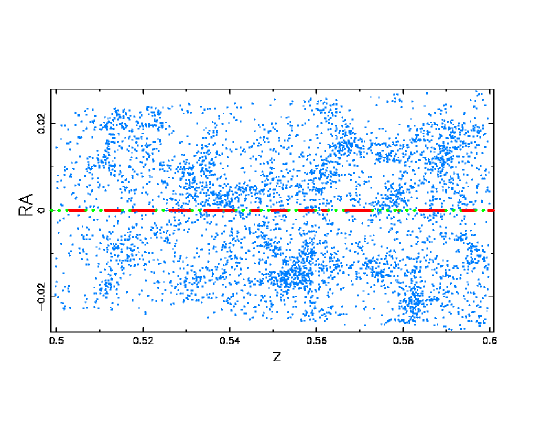
Figure 6: W1 field of VIPERS with z $\in$ (0.5,0.6). This plot contains 4716 galaxies (blue color). Two sequence of chords in the nearly Poissonian case are reported, the first chord is red (full line), the second chord is green (dotted line) .

6 Conclusions

Voronoi chords The PDF of the chord length distribution in PVT in the case $d=3$, where $d$ denotes the dimension, is reported as a numerical DF, see Table 5.7.4 in [11] or as a numerical PDF see Figure 2 in [15]. Here we derived a general expression in the case $d=3$ for chord length distribution in the case in which the Voronoi volumes are modeled by a Kiang function with variable shape parameter $c$. The generalized PDF is represented by eqn.(14) which covers the Poissonian case, $c=5$, the ordered case $c>5$ and the disordered case $c<5$.

Flat cosmology We derived an approximated relationship for the luminosity distance in spatially flat cosmology with pressureless matter and the cosmological constant as function of the redshift, see eqn.(22) and the inverse relationship, the redshift as function of the luminosity distance, see eqn.(23).

Astrophysical chord

In order to find $c$, the shape parameter of the Kiang’s function for volumes of cosmic voids, and $b$, the scale which fix the PDF for astrophysical chord, we processed two catalogs of cosmic voids, see Table 1. The exact PDF for astrophysical chord was derived, see eqns. (28) and (29). An approximated DF for astrophysical chord was deduced in the framework of the best minimax rational approximation, see eqns. (30) and (31). Two non linear equations, (33) and (32), allow the generation of random astrophysical chords. The inverse formula (23) allows the superposition of random astrophysical chords on two catalog of galaxies, see Figure 5 for 2dFGRS and Figure 6 for VIPERS.

References

- [1] T. Kiang, Random Fragmentation in Two and Three Dimensions, Z. Astrophys. 64 (1966) 433–439.
- [2] J.-S. Ferenc, Z. Néda, On the size distribution of Poisson Voronoi cells, Phys. A 385 (2007) 518–526.
- [3] L. Zaninetti, Chord distribution along a line in the local Universe , Revista Mexicana de Astronomia y Astrofisica 49 (2013) 117–126.
- [4] L. Zaninetti, M. Ferraro, On Non-Poissonian Voronoi Tessellations, Applied Physics Research 7 (2015) 108–124.
-
[5]
L. Zaninetti, Pade approximant and
minimax rational approximation in standard cosmology, Galaxies 4 (1) (2016)
4–24.
doi:10.3390/galaxies4010004.
URL http://www.mdpi.com/2075-4434/4/1/4 - [6] D. C. Pan, M. S. Vogeley, F. Hoyle, Y.-Y. Choi, C. Park, Cosmic voids in Sloan Digital Sky Survey Data Release 7, MNRAS 421 (2012) 926–934. arXiv:1103.4156, doi:10.1111/j.1365-2966.2011.20197.x.
- [7] J. Varela, J. Betancort-Rijo, I. Trujillo, E. Ricciardelli, The Orientation of Disk Galaxies around Large Cosmic Voids, ApJ 744 (2012) 82. arXiv:1109.2056, doi:10.1088/0004-637X/744/2/82.
- [8] J. Z. Ruan, M. H. Litt, I. M. Krieger, Pore size distributions of foams from chord distributions of random lines: Mathematical inversion and computer simulation, Journal of Colloid and Interface Science 126 (1) (1988) 93 – 100.
- [9] M. Abramowitz, I. A. Stegun, Handbook of Mathematical Functions with Formulas, Graphs, and Mathematical Tables, Dover, New York, 1965.
- [10] F. W. J. e. Olver, D. W. e. Lozier, R. F. e. Boisvert, C. W. e. Clark, NIST handbook of mathematical functions., Cambridge University Press. , Cambridge, 2010.
- [11] A. Okabe, B. Boots, K. Sugihara, S. Chiu, Spatial tessellations. Concepts and Applications of Voronoi diagrams, 2nd ed., Wiley, Chichester, New York, 2000.
- [12] M. Adachi, M. Kasai, An Analytical Approximation of the Luminosity Distance in Flat Cosmologies with a Cosmological Constant, Progress of Theoretical Physics 127 (2012) 145–152.
- [13] M. Colless, G. Dalton, S. Maddox, et al., The 2dF Galaxy Redshift Survey: spectra and redshifts, MNRAS 328 (2001) 1039–1063. arXiv:astro-ph/0106498.
- [14] B. Garilli, L. Guzzo, M. Scodeggio, M. Bolzonella, U. Abbas, C. Adami, S. Arnouts, J. Bel, D. Bottini, E. Branchini, A. Cappi, J. Coupon, O. Cucciati, I. Davidzon, G. De Lucia, S. de la Torre, P. Franzetti, A. Fritz, M. Fumana, B. R. Granett, O. Ilbert, A. Iovino, J. Krywult, V. Le Brun, O. Le Fèvre, D. Maccagni, K. Małek, F. Marulli, H. J. McCracken, L. Paioro, M. Polletta, A. Pollo, H. Schlagenhaufer, L. A. M. Tasca, R. Tojeiro, D. Vergani, G. Zamorani, A. Zanichelli, A. Burden, C. Di Porto, A. Marchetti, C. Marinoni, Y. Mellier, L. Moscardini, R. C. Nichol, J. A. Peacock, W. J. Percival, S. Phleps, M. Wolk, The VIMOS Public Extragalactic Survey (VIPERS). First Data Release of 57 204 spectroscopic measurements, A&A 562 (2014) A23. doi:10.1051/0004-6361/201322790.
- [15] L. Muche, Contact and chord length distribution functions of the Poisson-Voronoi tessellation in high dimensions, Adv. in Appl. Probab. 42 (1) (2010) 48–68.