Anisotropic multiple bounce models

Abstract

We analyze the Galileon ghost condensate implementation of a bouncing cosmological model in the presence of a non negligible anisotropic stress. We exhibit its structure, which we find to be far richer than previously thought. In particular, even restricting attention to a single set of underlying microscopic parameters, we obtain, numerically, many qualitatively different regimes: depending on the initial conditions on the scalar field leading the dynamics of the universe, the contraction phase can evolve directly towards a singularity, avoid it by bouncing once, or even bounce many times before settling into an ever-expanding phase. We clarify the behavior of the anisotropies in these various situations.

I Introduction

Observational cosmology Ade et al. (2016) mostly favors a primordial phase of single field slow-roll inflation Lemoine et al. (2008); Martin et al. (2014) (see Ref. Ijjas and Steinhardt (2016) for an alternative analysis of these data however). Moreover, inflation remains the most widely accepted paradigm permitting to solve the usual big bang puzzles of horizon, flatness and entropy Peter and Uzan (2013), leading to the currently observed homogeneous and isotropic universe. It also provides a natural means of producing linear perturbations with an almost scale-invariant spectrum. Non inflationary scenarios, however unfavored, have also been proposed, which yield an almost scale-invariant spectra for the scalar modes Battefeld and Peter (2015); Brandenberger and Peter (2016). The next step will perhaps come from observation of the tensor modes, whose signal could be used to discriminate various models, thus giving the necessary tools to discard or to accept non singular and non inflationary bouncing models.

The very first interest of a non-singular cosmology is of course that it avoids the singularity inherent to ever-expanding scenarios, thereby allowing to increase the size of the horizon as much as needed: with a long contraction phase followed by a bounce connecting to the presently expanding universe, any region can have been in causal contact with any other. Moreover, providing the contraction is decelerated for a sufficiently long time, the universe reaches the bounce in an almost flat condition. In short, bouncing models can also solve many of the above mentioned standard big bang puzzles in ways that differ from the inflationary solutions Peter and Pinto-Neto (2008).

The so-called “matter”-bounce Finelli and Brandenberger (2002); Brandenberger (2012) belongs to this particular class of models which may confront observations. During a contraction dominated by a field with negligible effective pressure $p\ll\rho$, the long wavelength scalar perturbations, originating in vacuum state, reach the bounce phase with a scale invariant spectrum Finelli and Brandenberger (2002). Another way to realize such a spectrum was proposed in Ref. Khoury et al. (2001): in this so-called ekpyrotic 5 dimensional model, the motion of 4 dimensional branes yields an effective 4 dimensional theory experiencing a contraction followed by an expansion phase in the Einstein frame; this model however needs to pass through a singular phase spoiling predictability Martin et al. (2002, 2003). In terms of the effective Friedmann-Lemaître-Robertson-Walker (FLRW) space-time, the dynamics can be mimicked by assuming the stress-energy tensor to be that of a scalar field $\phi$ with a negative potential describing the relative motion of the branes. In the proposal of Finelli and Brandenberger (2002), the exponential potential for the scalar field results in $w\equiv p/\rho\sim 0$, for a specific choice of parameters.

An important issue possibly plaguing any bouncing cosmological model, including in particular the matter bounce proposal, is the excessive growth of any initially small anisotropy deviation during contraction; this is usually referred to as the Belinsky, Khalatnikov and Lifshitz (BKL) Belinsky et al. (1970) instability. Since the anisotropic stress goes with the scale factor $a(t)$ as $a^{-6}$ (i.e. it can be seen as a fluid with effective equation of state $w_{\sigma}=1$), it can eventually dominate over the other fluid energy densities if the bounce is deep enough and/or the initial anisotropy is too large. This scenario assumes that the other fluids have equations of state $w<1$ ($w_{\mathrm{rad}}=\frac{1}{3}$ or $w_{\mathrm{mat}}\sim 0$), during the contraction phase. Note however that, if the anisotropy is initially very small, for instance resulting from initial quantum vacuum fluctuations, the bounce can take place before the anisotropy dominates over the other matter components Vitenti and Pinto-Neto (2012); Pinto-Neto and Vitenti (2014).

A way to solve the anisotropy problem in a contracting universe followed by a non-singular bounce, without merely setting its initial value to being vanishingly small, was suggested in Ref. Buchbinder et al. (2007). In this model, the potential was also chosen to be exponential so as to give the scalar field fluid an effective equation of state $w_{\phi}\gg 1$. As a result, this field dominates over the anisotropic stress during the entire contraction epoch, hence preventing any growth of the anisotropy compared to the other components. By the end of the contraction phase, a second scalar field takes over in a ghost condensate state, i.e., one for which the kinetic term may develop a non vanishing minimum inducing the canonical kinetic term in the Lagrangian to change sign for a finite amount of time. This leads to an effective equation of state $w_{\phi}<-1$, which drives the scale factor evolution to a halt: the universe goes through a bouncing phase. The condensate is responsible not only for the non-singular transition between contraction and expansion, but it also corrects the wavelength dependence of the scalar modes Arkani-Hamed et al. (2004): this is required because the ekpyrotic contraction yields a non scale-invariant spectrum for the perturbations.

Such a model has to face two problems. The first comes from the scalar field in the ghost condensate state: in order that it does not interfere with the background dynamics during the ekpyrotic contraction, it should be sufficiently diluted so as to dominate only during the final stages of contraction. The second issue concerns the long wavelength scalar perturbations, which may grow unstable after exiting the ekpyrotic phase Xue and Steinhardt (2011), leading to a spectrum very different from the observed quasi scale invariant one.

To address these issues, in yet another version of this new ekpyrotic model, the ghost condensate is obtained via a Galileon term that couples the scalar field with the metric Qiu et al. (2013). By means of two different functions of the scalar field, namely a negative potential $V(\phi)$ controlling the ekpyrotic phase, and a non-standard kinetic coupling $g(\phi)$ controlling the ghost condensate, it was then argued that the anisotropy growth is suppressed and the non-singular bounce is achieved even in the presence of small anisotropic deviation Cai et al. (2012, 2013). A curvaton mechanism Enqvist and Sloth (2002); Lyth and Wands (2002); Moroi and Takahashi (2001) is then invoked to finally produce scale invariant perturbations in the expansion phase.

Present calculations of the perturbations in models such as those discussed above have been done assuming an FLRW perturbed metric, under the assumption that the anisotropic stress can be made negligible for the relevant scales. On the other hand, if this assumption is not strictly valid and the background space-time is in fact Bianchi I, at least in some range of times, then it was shown Pereira et al. (2007) that the scalar, vector and tensor modes evolve in a coupled way already at first order. Even for an inflationary phase, this is known to yield possible effects in the resulting spectrum Pitrou et al. (2008), and it is only natural to expect a similar conclusion to hold in a contracting universe model. This could drastically modify any prediction for the final perturbation spectrum produced in such a model. Before addressing this question however, it is necessary to discuss the dynamics of the background itself.

The present work aims at exploring the evolution stemming from the theory proposed in Cai et al. (2013); as it happens, it is much richer than previously anticipated. The non singular models studied so far were for the most part based on one non-singular FLRW bounce. We show here that the highly non-linear features of the dynamical equations lead to a variety of unforeseen different scenarios. We exhibit four examples for which the underlying microscopic parameters are chosen as in Ref. Cai et al. (2013): they lead respectively to a singularity, one, two or even three bouncing stages depending on the chosen initial conditions. Our purpose is to exemplify these possibilities in order to open up and possibly constrain the relevant dynamical phase space of the acceptable backgrounds from which one will have to subsequently study the perturbations, to be eventually compared with the observational data.

The paper is organized as follows: in the following Section, we review the model of Ref. Cai et al. (2013), expand the relevant equations of motion in the Bianchi I case and set the dynamical system to be solved numerically. Section III is devoted to a presentation of our numerical solutions for different background behaviors, pointing out the main phenomenology behind the different dynamics. Section IV returns to the basic equations and discusses the role, influence and evolution of the anisotropy in multiple bounce scenarios, together with a discussion on the expected effects of changing the model parameters. Section V summarizes our findings and offers some concluding remarks and expectations on the power spectrum and its properties in these models.

In what follows, we work in units such that $\hbar=c=1$ and the reduced Planck mass is $M_{{}_{\mathrm{P}}}=1/\sqrt{8\pi G_{{}_{\mathrm{N}}}}$. The metric signature is $(+,-,-,-)$. Throughout the paper, the scale factor is normalized to unity at the first bouncing point.

II General equations

Our starting point is to assume a Galileon scalar field $\phi$ minimally coupled to Einstein gravity, i.e.

$$\mathcal{S}=\int\mathrm{d}^{4}\sqrt{-g}\left(\frac{1}{2}M_{{}_{\mathrm{P}}}^{2}R+\mathcal{L}\right),$$ (1)

where the scalar field Lagrangian is taken to be

$$\mathcal{L}\left[\phi\left(x\right)\right]=K(\phi,X)+G(\phi,X)\Box\phi,$$ (2)

$K$ and $G$ being functions of the field itself and its canonical kinetic term

$$X\equiv\frac{1}{2}\partial_{\mu}\phi\partial^{\mu}\phi,$$ (3)

and $\Box\phi\equiv g^{\mu\nu}\nabla_{\mu}\nabla_{\nu}\phi$ where $\nabla_{\nu}$ represents the torsion-free covariant derivative compatible with the metric $g_{\mu\nu}$.

Variations of $\mathcal{L}$ yields the relevant energy momentum tensor

$$T^{\phi}_{\mu\nu} = (-K+2XG_{,\phi}+G_{,X}\nabla_{\sigma}{X}\nabla^{\sigma}\phi)g_{\mu\nu}$$ (4)

$$+(K_{,X}+G_{,X}\Box\phi-2G_{,\phi})\nabla_{\mu}\phi\nabla_{\nu}\phi$$

$$-G_{,X}(\nabla_{\mu}{X}\nabla_{\nu}\phi+\nabla_{\nu}{X}\nabla_{\mu}\phi),$$

where the notations $F_{,\phi}$ and $F_{,X}$ stands for derivatives of whatever $F$ stands for with respect to $\phi$ and $X$, respectively.

Following Ref. Cai et al. (2013), we choose

$$K(\phi,X)=M_{{}_{\mathrm{P}}}^{2}\left[1-g(\phi)\right]X+\beta X^{2}-V(\phi),$$ (5)

with the positive-definite parameter $\beta$ ensuring the kinetic term to be bounded from below at high energy scales and we assume the scalar field $\phi$ is dimensionless, hence the Planck mass coefficient on the first term. The arbitrary functions in (5) must be such as to render an ekpyrotic contraction phase together with a non singular ghost condensate dominated bounce possible. As explained in Cai et al. (2013), an acceptable choice is provided by

$$g(\phi)=\frac{2g_{0}}{\mathrm{e}^{-\sqrt{\frac{2}{p}}\phi}+\mathrm{e}^{b_{g}\sqrt{\frac{2}{p}}\phi}},$$ (6)

with $g_{0}>1$, $p>0$ and $b_{g}$ dimensionless constants, while the potential can be taken as

$$V(\phi)=-\frac{2V_{0}}{\mathrm{e}^{-\sqrt{\frac{2}{q}}\phi}+\mathrm{e}^{b_{\mathrm{v}}\sqrt{\frac{2}{q}}\phi}},$$ (7)

where $V_{0}>0$ is constant with dimension of $({\rm mass})^{4}$ and two other dimensionless constants $q$ and $b_{\mathrm{v}}$. This negative-definite potential reduces to the exponential form of the ekpyrotic scenario Finelli and Brandenberger (2002) for large values of $\phi$. Finally, the function $G(\phi,X)$ is of the Galileon type Deffayet et al. (2009), again chosen in agreement with Cai et al. (2013) as $G(X)=\gamma X$, with $\gamma$ is a positive dimensionless constant.

With the matter content fixed, the system is complete once we give the relevant geometrical symmetries. This we do by assuming a flat, homogeneous and anisotropic universe, whose dynamics is described by a Bianchi I metric, namely

$$\mathrm{d}s^{2}=\mathrm{d}t^{2}-a^{2}(t)\sum_{i}\mathrm{e}^{2\theta_{i}(t)}\mathrm{d}x^{i}\mathrm{d}x^{i},$$ (8)

the average scale factor $a(t)$ permitting to define a mean Hubble rate through $H\equiv\dot{a}/a$, the “dot” denoting time derivative with respect to cosmic time $t$.

The equation of motion of the scalar field $\phi$ is derived from the Lagrangian (2) and can be cast in the form of a modified Klein-Gordon equation, namely

$$\mathcal{P}\ddot{\phi}+\mathcal{D}\dot{\phi}+V_{,\phi}=0,$$ (9)

where the functions $\mathcal{P}$ and $\mathcal{D}$ depend on both the scalar field itself and the geometry; they are respectively given by

$$\mathcal{P}=(1-g)M_{{}_{\mathrm{P}}}^{2}+6\gamma H\dot{\phi}+3\beta\dot{\phi}^{2}+\frac{3\gamma^{2}}{2M_{{}_{\mathrm{P}}}^{2}}\dot{\phi}^{4},$$ (10)

and

$$\mathcal{D}= 3(1-g)M_{{}_{\mathrm{P}}}^{2}H+\left(9\gamma{H}^{2}-\frac{1}{2}M_{{}_{\mathrm{P}}}^{2}g_{,\phi}\right)\dot{\phi}+3\beta{H}\dot{\phi}^{2}$$

$$-\frac{3}{2}(1-g)\gamma\dot{\phi}^{3}-\frac{9\gamma^{2}H\dot{\phi}^{4}}{2M_{{}_{\mathrm{P}}}^{2}}-\frac{3\beta\gamma\dot{\phi}^{5}}{2M_{{}_{\mathrm{P}}}^{2}}-\frac{3}{2}\gamma\sum_{i}\dot{\theta}_{i}^{2}\dot{\phi}.$$ (11)

The parameters of the model are $g_{0}$, $V_{0}$, $b_{g}$, $b_{\mathrm{v}}$, $p$, $q$, $\beta$, $\gamma$ all real, positive and assumed non vanishing. Without lack of generality, we set $M_{{}_{\mathrm{P}}}\to 1$ for the rest of this work.

Defining the shear

$$\sigma^{2}=\sum_{i}\dot{\theta}_{i}^{2},$$ (12)

the Friedmann equations follow from the stress-energy tensor (4); they are

$$H^{2}=\frac{\rho_{\phi}}{3}+\frac{\sigma^{2}}{6},$$ (13)

for the constraint, and

$$\dot{H}=-\frac{\rho_{\phi}+p_{\phi}}{2}-\frac{1}{2}\sigma^{2}.$$ (14)

In (13) and (14), the energy density $\rho_{\phi}$ and pressure $p_{\phi}$ of the scalar field are given by

$$\rho_{\phi} = \frac{1}{2}(1-g)\dot{\phi}^{2}+\frac{3}{4}\beta\dot{\phi}^{4}+3\gamma H\dot{\phi}^{3}+V(\phi),$$ (15)

$$p_{\phi} = \frac{1}{2}(1-g)\dot{\phi}^{2}+\frac{1}{4}\beta\dot{\phi}^{4}-\gamma\dot{\phi}^{2}\ddot{\phi}-V(\phi).$$ (16)

Finally, as discussed in the introduction, the shear evolves as

$$\sigma^{2}=\sigma^{2}_{\mathrm{ini}}\left(\frac{a_{\mathrm{ini}}}{a}\right)^{6},$$ (17)

i.e., as a stiff-matter fluid, where the subscript “ini” denotes an arbitrary initial time. For future convenience, we shall refer to the quantity

$$\rho_{\sigma}\equiv\frac{\sigma^{2}}{2}=p_{\sigma}$$ (18)

as the energy density and pressure associated to the anisotropy.

III Numerical solutions

The dynamical equations presented in the last section can be recast into a system of first order differential equations, namely

$$\dot{\phi} =\varphi,$$ (19)

$$\dot{\varphi} =-\frac{\mathcal{D}\varphi}{\mathcal{P}}-\frac{V_{,\phi}}{\mathcal{P}},$$ (20)

$$\dot{H} =-\frac{\rho_{\phi}+p_{\phi}}{2}-\frac{\sigma^{2}_{\mathrm{ini}}}{2}\left(\frac{a_{\mathrm{ini}}}{a}\right)^{6},$$ (21)

$$\dot{a} =aH,$$ (22)

where we have introduced a new variable $\varphi$ to reduce the system order and used Eqs. (9), (14), (17) and the definition of the mean Hubble rate $H$. We assume the underlying parameters are those already chosen in Cai et al. (2013), so the numerical solutions presented below will be comparable with this previous work. We have

$$V_{0} =10^{-7}M_{{}_{\mathrm{P}}}^{4}, g_{0} =1.1,$$

$$b_{\mathrm{v}} =5, b_{g} =0.5,$$

$$p =0.01, q =0.1,$$

$$\beta =5, \gamma =10^{-3}.$$

The initial conditions are given by the set

$$\theta=(\phi_{\mathrm{ini}},\;\varphi_{\mathrm{ini}})\ \ \ \hbox{and}\ \ \ \sigma^{2}_{\mathrm{ini}}=5\times 10^{-12},$$ (23)

with $\varphi_{\mathrm{ini}}$ chosen in such a way that the kinetic contribution $\propto\varphi_{\mathrm{ini}}^{2}$ be comparable to the shear contribution at the initial time (recall we fixed $a_{\mathrm{ini}}=1$), while $H$ is given by the constraint (13), namely

$$H_{\mathrm{ini}}=-\sqrt{\frac{{\rho_{\phi}}_{\mathrm{ini}}}{3}+\frac{1}{6}\sigma^{2}_{\mathrm{ini}}},$$ (24)

where ${\rho_{\phi}}_{\mathrm{ini}}$ is obtained with Eq. (15) evaluated at $\phi_{\mathrm{ini}}$ and $\varphi_{\mathrm{ini}}$. Finally, note that we have omitted the scale factor $a$ since it enters explicitly only in the expression for the shear in Eq. (17) through the combination $\sigma_{\mathrm{ini}}a_{\mathrm{ini}}^{3}$: without loss of generality, one can renormalize the initial shear to account for the initial value of the scale factor, which can thus be chosen as $a_{\mathrm{ini}}=1$ for simplicity.

Reference Cai et al. (2013) considered the presence of a matter component, $p\ll\rho$, assumed to produce the initially scale-invariant spectrum. Here, we want to focus on the bounce itself, or the behavior of the scale factor in general when the universe is dominated by the scalar field. This means we begin our analysis at a time for which we assume the dust fluid contribution has already turned negligible, having been overcome by the other components when we set our initial conditions. In other words, for $a<a_{\mathrm{ini}}$ (we set initial conditions in a contracting epoch), the matter fluid is negligible and we shall accordingly forget it altogether.

In the numerical solutions presented below in Figs. 1 through LABEL:Fig:rho_sigma, the time $t$ is expressed in units of $10^{4}M_{{}_{\mathrm{P}}}^{-1}$ and the Hubble rate $H$ in units of $10^{-4}M_{{}_{\mathrm{P}}}$. In order to compare the solutions with the same reference point, we always set the initial time to $t_{\mathrm{ini}}=0$. The estimated absolute error in the calculations shown are of order $\mathcal{O}(10^{-10})$ during the contraction and expansion epochs, and $\mathcal{O}(10^{-7})$ during the bounce phase. Since we are interested in the potential effects of a remaining sub-dominant anisotropy during the bounce, we consider in what follows initial conditions such that the effective equation of state (EoS) is not very large at the beginning, i.e., we are assuming that only a weak ekpyrotic phase, where the EoS is only slightly above one, has taken place in our scenario before we set our initial conditions.

III.1 One bounce scenario

The single bounce scenario is the most widely discussed background evolution for bouncing cosmologies. The background evolves dominated by the scalar field during contraction, passes through the ghost condensate phase, makes a single non singular bounce and enters an ever lasting expansion phase afterwards, as exemplified in Fig. 1. These numerical solutions were obtained for $\phi_{\mathrm{ini},1}=-2.5$ and $\phi_{\mathrm{ini},2}=-3.0$, with $\varphi_{\mathrm{ini}}=8\times 10^{-6}$ in both cases. As noted earlier, the initial shear value is close to the kinetic term $\varphi^{2}\sim\times 10^{-11}$, and is subsequently diminished (in comparison to $\rho$) during the ekpyrotic phase.

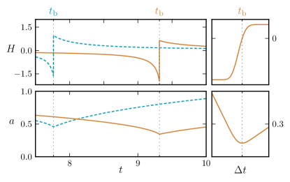
Figure 1: Time evolution of the Hubble constant $H$ (top left) and scale factor $a$ (bottom left) for $\varphi_{\mathrm{ini}}=8\times 10^{-6}$ and two different values of $\phi_{\mathrm{ini}}$: $\phi_{\mathrm{ini}}=-3$ (full brown) and $\phi_{\mathrm{ini}}=-2.5$ (dashed blue). The bounce times are marked as $t_{\mathrm{b}}$. The discontinuity is only apparent and a mere consequence of the fact that the relevant time scale is extremely short for the fast bounce that takes place in this theory: the right panels show the details of this actually smooth transition (shown only for $\phi_{\mathrm{ini}}=-3.5$) over the much smaller time interval of $\Delta t=10^{-4}$ around the bounce time ${\color[rgb]{0.8,0.5,0.2}t_{\mathrm{b}}}$. Although not shown explicitly on later plots, all the following curves are in fact smooth on the relevant scales as we did check for all cases.

The ghost condensate and ekpyrotic phases are presented in Fig. 2 where the time development of the kinetic term coefficient $g$ and the potential $V$ are presented. Before the bounce takes place, the scalar field is driven by the potential which becomes very negative all through the ekpyrotic phase, until $g$ takes over, at which point the bounce occurs. Fig. 3 shows, for this case and the following (with more than one bounce taking place), the time evolution of the energy contained in the scalar field and in the shear. The top panel is for the case at hand: the difference between $\rho_{\phi}$ and $\rho_{\sigma}$ is entirely due to $V(\phi)$ in this case, and as expected, the shear contribution decreases with respect to that of the field.

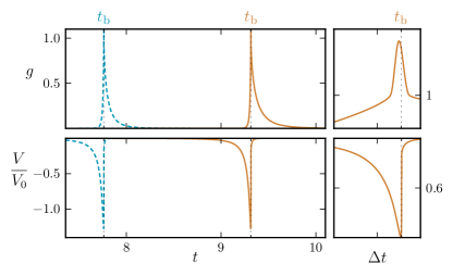
Figure 2: Time development of the kinetic function $g\left[\phi\left(t\right)\right]$ (top left) and potential $V\left[\phi\left(t\right)\right]/V_{0}$ (bottom left), with the same convention as Fig. 1. The ghost condensate phase begins as soon as $g(\phi)\geq 1$. The right panel shows how smooth the transition goes when looked at on shorter timescales.

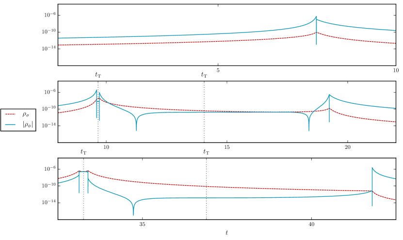
Figure 3: Comparative evolution of the energy densities for the anisotropy, $\rho_{\sigma}$ (red dashed) and the scalar field, $\rho_{\phi}$ (blue full) for the initial conditions $\{\phi_{\mathrm{ini}}=-2.5,\ \varphi_{\mathrm{ini}}=8\times 10^{-6}\}$ (top, single bounce), $\{\phi_{\mathrm{ini}}=-3.5,\ \varphi_{\mathrm{ini}}=8\times 10^{-6}\}$ (middle, two bounces) and $\{\phi_{\mathrm{ini}}=1.9,\ \varphi_{\mathrm{ini}}=-10^{-6}\}$ (bottom, three bounces). The initial anisotropic stress for all the plots is $\sigma^{2}_{\mathrm{ini}}=5\times 10^{-12}$. The indicated $t_{\mathrm{T}}$ are the turning points at which the scalar field goes through the maximum of $g(\phi)$.

Reducing the shear is what the ekpyrotic phase is made for. Indeed, with the potential (7), there exists an attractor solution with EoS for the scalar field $w_{\phi}$

$$w_{\phi}\approx-2+\frac{2}{3q},$$ (25)

while on the other hand, Eq. (17) implies that the EoS of the shear is $w_{\sigma}=1$. For small values of $q$, as the one we are interested in and have chosen for the numerical calculations, the shear can never dominate during contraction. Although we did not start on the attractor (25), we obtained that behavior for two different choices of initial conditions for $\phi_{\mathrm{ini}}$. The more negative $\phi_{\mathrm{ini}}$, the longer the contraction phase, because the scalar field begins farther away from the ghost condensate state that permits the bounce. There is a degeneracy in the initial condition space, since one could achieve a similar behavior by changing $\varphi_{\mathrm{ini}}$, an initially small velocity for the field leading to a longer contraction phase as it takes more time to reach the ghost condensate phase.

At first sight, one is tempted to conclude from the previous discussion that $\phi_{\mathrm{ini}}$ or $\varphi_{\mathrm{ini}}$ could be chosen as small as one wishes in order to yield a longer contraction phase and varying the bounce characteristic features. As it turns out, this is not the case at all: as we show in the following section, changing the initial conditions produces drastically different solutions involving more than one bounce.

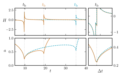
Figure 4: Evolution of the Hubble parameter $H$ (top left) and the scale factor $a$ (bottom left) for the two different initial conditions: $\phi_{\mathrm{ini}}=-3.5$ (full yellow) and $\phi_{\mathrm{ini}}=-3.49$ (blue dashed). The bounces are marked as $t_{\mathrm{b}}$. The first bounce of the two solutions are indistinguishable on the figure (numerically extremely close), but the solutions then drift away and bifurcate, yielding a second bounce at very different times, first for $\phi_{\mathrm{ini}}=-3.5$, then for $\phi_{\mathrm{ini}}=-3.49$. This indicates an extreme sensibility in the initial conditions that has never been discussed in such a context. The plots on the right detail what happens during the first time the system goes through the ghost condensate phase, with a time scales of the plot taken as $\Delta t\approx 3$ around ${\color[rgb]{0.8,0.5,0.2}t_{\mathrm{b}}}$.

III.2 Two bounce case

Figure 4 illustrates what happens if one keeps decreasing $\phi_{\mathrm{ini}}$, trying to trigger a longer contraction phase: one reaches a region in parameter space in which the Universe instead experiences two bounces. The universe contracts, bounces, expands again, passes through a maximum, starts contracting again and moves towards a second bounce, from which it finally expands forever. For that to happen, the scalar field must go twice through the ghost condensate phase, a possibility which was always assumed hard to achieve, whereas in fact, we found it actually goes through this phase three times (see Fig. 5) even though only two bounces took place.

This evolution is exemplified by $\varphi_{\mathrm{ini}}=8\times 10^{-6}$ and the two initial field conditions $\phi_{\mathrm{ini},1}=-3.49$ and $\phi_{\mathrm{ini},2}=-3.50$, whose subsequent time development is depicted in Figs. 4 and 5.

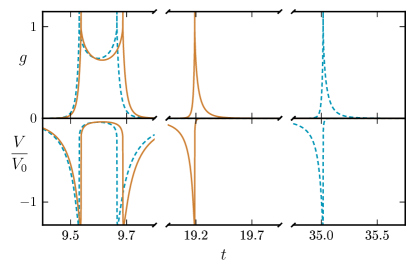
Figure 5: Time developments of $g(\phi)$ (top) and the potential $V(\phi)$ (bottom). The two solutions are for $\phi_{\mathrm{ini}}=-3.5$ (full yellow), $\phi_{\mathrm{ini}}=-3.49$ (blue dashed), both with $\varphi_{\mathrm{ini}}=8\times 10^{-6}$. As in Fig. 2 the peaks only appear discontinuous but in actuality are smooth.

The behavior we find here is due to the existence of a turning point for $\phi$, marked as $t_{\mathrm{T}}$ in Fig. 3. At this point, the scalar field passes through the first ghost condensate phase while still contracting. It eventually returns and goes back to pass through the top of the potential $g(\phi)$ another time. Then, the universe bounces.

In Fig. 5, we show that after the first bounce took place, the expansion phase is again dominated by the ekpyrotic potential $V(\phi)$. As we mentioned before, during the ekpyrotic phase, the effective EoS of the scalar field is built to be larger than that of the anisotropy. This means that, during contraction, the scalar field dominates for small values of $a$, but conversely also that during expansion, the anisotropy becomes more and more important. This is illustrated in Fig. 3 where the shear domination after the first bounce is clearly visible.

With the expansion dominated by the anisotropy, $\phi$ reaches a second turning point, while $H$ became negative again. This is the beginning of the second contraction phase that will eventually drive $\phi$ into the ekpyrotic phase again (see the third peak of Fig. 5), thereby reducing the shear contribution again. When the scalar field again reaches the peak of $g(\phi)$, (third ghost condensate phase), this triggers the bounce in an even more isotropic state.

From that example, one can envisage two possible scenarios. Without the first turning point, the Universe would have gone through a ghost condensate phase without triggering a bounce and a singularity would have ensued. It is often stated that one of the most dangerous effect that can prevent a bounce from taking place is the uncontrolled growth of anisotropy. We found that the scalar field initial conditions are also important in order to ensure the bounce can occur. Below we also argue that in fact, it is thanks to the existing anisotropy that the universe does not plunge straightforwardly into a singularity. The second scenario is when conditions are such as to avoid the second turning point altogether. In that case, the last expansion epoch begins anisotropic: the ekpyrotic contraction, although controlling the relative shear decay, is not sufficient as the multiple bounces subsequently spoil its effect. A phase of ekpyrotic contraction is thus not necessarily enough to guarantee that the resulting universe, after the bounce, expands isotropically, the scalar field initial conditions playing a crucial role in the overall evolution of the universe.

III.3 Three bounces

Our final example is rather counter intuitive. It begins with an anisotropic contraction phase not leading to a BKL instability and resulting into a final expansion phase even more isotropic than the previous cases (see Fig. 3). To produce this scenario, we tune the value of $\phi_{\mathrm{ini}}$, chosen positive, keeping the amount of initial anisotropy as before, $\sigma^{2}_{\mathrm{ini}}=5\times 10^{-12}$, and we set $\varphi_{\mathrm{ini}}=-10^{-6}$, together with the two field values $\phi_{\mathrm{ini},1}=1.9$ and $\phi_{\mathrm{ini},2}=1.9001$, noting that since the initial field time derivative is smaller, the anisotropy is initially larger than the kinetic term $\varphi^{2}=10^{-12}$.

The usual ekpyrotic approach consists in beginning with the ekpyrotic phase so as to lower, dissolve really, the relative shear contribution immediately, during the initial contraction, thereby solving the anisotropy problem. The case here is completely different, as we start with $\phi_{\mathrm{ini}}>0$ and $\varphi_{\mathrm{ini}}<0$ so that the scalar field starts evolving from the right hand side of the potential $V(\phi)$ and of $g(\phi)$. This means that, contrary to the cases discussed above, we do not begin the evolution of the universe with the ekpyrotic phase: this phase only happens after the first ghost condensate peak, as shown in Fig. 6.

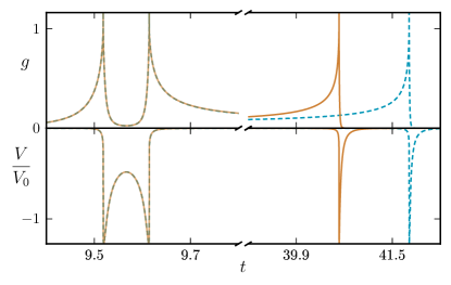
Figure 6: Time developments of $g(\phi)$ (top) and the potential $V(\phi)$ (bottom). The three peaks leads to the three bounces of Fig. 7 with initial conditions given by $\phi_{\mathrm{ini}}=1.9001$ (full yellow), and $\phi_{\mathrm{ini}}=1.900$ (blue dashed). The fine-tuning required on $\phi_{\mathrm{ini}}$ reflects the fact that it is extremely difficult to obtain a final isotropically expanding state when beginning with a shear dominated contracting universe. In fact, almost any other initial condition leads to a singularity.

As in the two bounce case of Sec. III.2, the existence of a turning point is mandatory for the observed behavior. Otherwise, the universe merely collapses into a singularity.

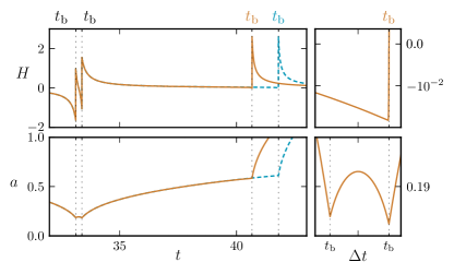
Figure 7: Evolution of the Hubble constant $H$ (top left) and the scale factor $a$ (bottom left) for the same initial conditions as in Fig. 6. The other initial conditions for both cases are $\varphi_{\mathrm{ini}}=-10^{-6}$ and $\sigma^{2}_{\mathrm{ini}}=5\times 10^{-12}$. The first two bounces happen at roughly the same time for both initial conditions, and the solutions then drift away as in the previous example before reaching the third bounce. The top right panels emphasizes the smoothness of the evolution of $H$ around the third bounce in the case $\phi_{\mathrm{ini}}=1.9001$ (the other has a similar shape). It turns out the Hubble scale becomes slightly negative only, and for a very limited amount of time, indicating a very short contraction phase. The bottom left panel details the first two bounces for the case $\phi_{\mathrm{ini}}=1.9001$. The time scale of the plots are $\Delta t\approx 10^{-3}$ around the third bounce, ${\color[rgb]{0.8,0.5,0.2}t_{\mathrm{b}}}$ (top right panel) and $\Delta t\approx 10^{-1}$ around the first two bounces, indicated by $t_{\mathrm{b}}$ (bottom right). Enlarging more the time scale on this latter plot shows the bounces are, again, smooth and only appear discontinuous because of the time scales used to represent them.

The presence of three ghost condensate phases, i.e., the peaks of $g(\phi)$ in Fig. 6, leads to the three bounces of Fig. 7. The first contraction, containing no ekpyrotic phase, is completely dominated by the anisotropy (Fig. 3). After the first bounce, the universe expands ekpyrotically as it reaches the first peak of $V(\phi)$, Fig. 6. During this ekpyrotic expansion, $\phi$ reaches a turning point and $H$ changes sign, initiating the second contraction.

After the second contraction, the universe once again goes through the ghost condensate phase and another bounce occurs. The ensuing expansion is still anisotropic, until the scalar field reaches another turning point, at which point the universe begins contracting for the third time while $\phi$ climbs back up in $g(\phi)$. During this third contraction, which is not ekpyrotic-like, the scalar field energy contribution appears to grow faster than the anisotropy, as shown in Fig. 3. The scenario ends after $\phi$ crosses the last peak of $g(\phi)$, and the universe bounces for the third time.

As can be seen in Fig. 7, the third contraction is a very short phase with a minimum Hubble scale of $H_{\mathrm{min}}\approx 10^{-2}$ before the third bounce. Because the contraction was shorter than the expansion, the anisotropy is more diluted. At the same time, $\phi$ starts to grow faster than the anisotropy. This is a very unexpected behavior. As we can see in Fig. 6, there is no ekpyrotic potential contribution before the third bounce to render the effective EoS of the scalar field larger than that of the anisotropy.

The final stage of the process described above is the third bounce itself, at which point the scalar field overcomes the anisotropy, leading the universe to the required isotropic expansion. Even though the expansion in dominated by the scalar field in the ekpyrotic phase (Fig. 6), the difference between the energy densities is large enough that the anisotropy does not end up dominating.

III.4 Singular solutions

Despite the presence of an ekpyrotic phase and a ghost condensate regime, the existence of a bouncing solution is not guaranteed. In Fig. 8, we show a sequence of solutions for different values of $\phi_{\mathrm{ini}}$, assuming in all cases $\varphi_{\mathrm{ini}}=8\times 10^{-6}$ and $\sigma^{2}_{\mathrm{ini}}=5\times 10^{-12}$, some solutions being regular and bouncing, other contracting endlessly to a singularity, for initial values of the scalar field not too far away from one another. The list of initial conditions used here is $\phi_{\mathrm{ini},1}=-2.5$, $\phi_{\mathrm{ini},1}=-3.5$, $\phi_{\mathrm{ini},1}=-4.0$, and $\phi_{\mathrm{ini},1}=-4.5$.

This last case leads us to conclude that the more negative $\phi_{\mathrm{ini}}$, the longer the contraction phase and the larger the anisotropy when the system reaches the ghost condensate state. Fig. 8 shows the transitions from one bounce, two bounces and no bounce solutions while decreasing $\phi_{\mathrm{ini}}$. As it turns out, the singular solution is not the limit of a single bounce case, but rather a two-bounce situation in which the second bounce is failed, the Hubble rate suddenly increasing while the scalar field passes through the ghost condensate phase, but not enough to render it positive, so the ghost condensate epoch terminates in a still contracting phase, and the universe has subsequently no chance to return to expansion.

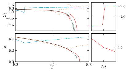
Figure 8: Time evolution of the Hubble constant, $H$ (top left), and the scale factor, $a$ (bottom left), for $\dot{\phi}_{\mathrm{ini}}=-8\times 10^{-6}$ and $\sigma^{2}_{\mathrm{ini}}=5\times 10^{-12}$, with four different initial conditions on $\phi_{\mathrm{ini}}$ leading respectively to one bounce (blue dot-dashed line, $\phi_{\mathrm{ini}}=-2.5$), two bounces (yellow small dashed line, $\phi_{\mathrm{ini}}=-3.5$) and singular solutions (red full line, $\phi_{\mathrm{ini}}=-4.0$ and green long dashed line, $\phi_{\mathrm{ini}}=-4.5$). The right panel details what happens at the point where the dynamics would lead to a bounce in a regular solution: the system goes through the ghost condensate, but for an insufficient amount of time, so that even though $H$ increases (top right), changing the slope of $a$ (bottom right), it remains negative, leading ultimately to an unavoidable singularity. The time scale for the right panel plots is $\Delta t=10^{-4}$ around $t=9.7$.

IV Discussion

The main feature enabling the universe described by our model to bounce a few times is the possibility of one or more turning points, making the scalar field climb the potentials more than once. Let us now examine their properties and the consequences they can have on the evolution of the universe.

As discussed earlier, a turning point at time $t_{\mathrm{T}}$ is characterized by $\varphi(t_{\mathrm{T}})=0$ and $\dot{\varphi}(t_{\mathrm{T}})<0$, if $\phi(t_{\mathrm{T}})$ is a local maximum or $\dot{\varphi}(t_{\mathrm{T}})>0$, if $\phi(t_{\mathrm{T}})$ is a local minimum. This solution should necessarily satisfy the Friedmann equation (13). Substituting $\varphi=\dot{\phi}=0$ in Eq. (13) and defining

$$y\equiv\mathrm{e}^{\sqrt{\frac{2}{q}}\phi},$$ (26)

the Friedmann constraint reads:

$$y^{-1}+y^{b_{\mathrm{v}}}+\frac{2}{3}V_{0}\left(H^{2}-\displaystyle\frac{\sigma^{2}}{6}\right)^{-1}=0.$$ (27)

Demanding that there exists a turning point means that there should be at least one root to the above equation.

Let us define $f(y)$ from Eq. (27), namely

$$f(y)=y^{-1}+y^{b_{\mathrm{v}}}+\frac{2}{3}V_{0}\left(H^{2}-\displaystyle\frac{\sigma^{2}}{6}\right)^{-1}.$$ (28)

The range of variation of this function follows from that of $\phi$, so that $y\rightarrow 0$ implies $\phi\rightarrow-\infty$, and $y\rightarrow\infty$ leads to $\phi\rightarrow\infty$. One can easily check that

$$\lim_{y\rightarrow 0}f(y)=\infty\ \ \ \ \hbox{and}\ \ \ \ \lim_{y\rightarrow\infty}f(y)=\infty,$$ (29)

so that if there exists $\bar{y}$ such that $f(\bar{y})<0$, then, by virtue of Bolzano’s theorem on intermediate values for continuous functions, one is guaranteed that $f(y)$ possesses at least two roots, which we call respectively $\phi^{*}_{1}\in\big{]}-\infty,\sqrt{q/2}\ln\bar{y}\big{]}$ and $\phi^{*}_{2}\in\big{[}\sqrt{q/2}\ln\bar{y},\infty\big{[}$, eligible as turning points.

The condition $f(\bar{y})<0$ is only possible provided the condition

$$H^{2}<\frac{\sigma^{2}}{6}.$$ (30)

holds. This last expression shows that the anisotropy plays a non trivial part in the existence of the turning point, enabling $f(y)$ to have a root. For an isotropic universe, the shear by definition vanishes, $\sigma^{2}=0$ and the system can only bounce once. By continuity, for very small values of the initial anisotropy, the initial condition on $\phi$ dictates whether it is possible that Eq. (30) is satisfied. The higher the shear, the more likely one encounters a regime during which Eq. (30) is valid during the evolution and thus, the more likely the existence of turning points. Contrary to the common lore, a high value of the primordial anisotropy may therefore not necessarily spoil the bouncing scenario, or even the resulting isotropic expansion.

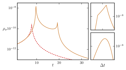
Figure 9: Evolution of the effective energy density for the anisotropic stress, $\rho_{\sigma}$ (left) for $\varphi_{\mathrm{ini}}=8\times 10^{-6}$ and $\sigma^{2}_{\mathrm{ini}}=5\times 10^{-12}$ with $\phi_{\mathrm{ini}}=-2.5$ (red dashed line, single bounce) and $\phi_{\mathrm{ini}}=-3.5$ (full yellow line, two bounce case), previously discussed in Sections III.1 and III.2 respectively. The top right panels shows a detail of the first peak of the anisotropy energy density in the two bounces case. We can see the effect of the first turning point and the ekpyrotic expansion in the increase of the anisotropy before the first bounce, highest peak. The bottom right panel is a zoom in of the highest peak to emphasize the smoothness of the numerical solutions. The time scales of the relevant plots are respectively $\Delta t\approx 10^{-1}$ around $t=9.7$ (top right panel) and $\Delta t\approx 10^{-4}$ around $t=9.7$ (bottom right panel).

From the modified Klein-Gordon equation (9), at the turning point, we have:

$$\dot{\varphi}=-\frac{V_{,\phi}}{(1-g)}.$$ (31)

Differentiating $V(\phi)$, one can show that the sign of $V_{,\phi}$ is opposite to that of $v$, defined through

$$v\equiv 1-b_{\mathrm{v}}\mathrm{e}^{(1+b_{\mathrm{v}})\sqrt{\frac{2}{q}}\phi},$$ (32)

as can be seen from

$$V_{,\phi}=-2V_{0}\sqrt{\frac{2}{q}}\left[1+\mathrm{e}^{\sqrt{\frac{2}{q}}(1+b_{\mathrm{v}})\phi}\right]^{-2}v.$$ (33)

The definition (32) implies that $v$ is positive (respectively negative) if $\phi$ is less (resp. greater) than $\phi_{\mathrm{lim}}$ defined by

$$\phi_{\mathrm{lim}}=-\sqrt{\frac{q}{2}}\frac{\ln\left(b_{\mathrm{v}}\right)}{1+b_{\mathrm{v}}}.$$ (34)

From Eq. (31), $\mathrm{sign}(\dot{\varphi})=\mathrm{sign}(v)$, since outside the ghost condensate phase, $(1-g)>0$. We therefore conclude that, at the turning point, $\dot{\varphi}(t_{\mathrm{T}})$ is positive (resp. negative) if $\phi(t_{\mathrm{T}})$ is less (resp. greater) than $\phi_{\mathrm{lim}}$.

Evaluating Eq. (28) in $y_{\mathrm{lim}}=y(\phi_{\mathrm{lim}})=b_{\mathrm{v}}^{-1/(1+b_{\mathrm{v}})}$, we have

$$f(y_{\mathrm{lim}})=b_{\mathrm{v}}^{\frac{1}{1+b_{\mathrm{v}}}}+b_{\mathrm{v}}^{-\frac{b_{\mathrm{v}}}{1+b_{\mathrm{v}}}}+\frac{2}{3}\frac{V_{0}}{H^{2}-\displaystyle\frac{\sigma^{2}}{6}},$$ (35)

so that, for the chosen parameters, we obtain

$$b_{\mathrm{v}}^{\frac{1}{1+b_{\mathrm{v}}}}+b_{\mathrm{v}}^{-\frac{b_{\mathrm{v}}}{b_{\mathrm{v}}+1}}\approx 1.5\sim\mathcal{O}(1).$$

As can be read from the graph, $H^{2}$ is of order $10^{-11}-10^{-12}$ around the turning point (marked as $t_{\mathrm{T}}$ in Fig. 3), whereas $\rho_{\sigma}\approx 10^{-10}$, so we can neglect the former with respect to the latter and assume $H^{2}<\sigma^{2}/6$ for an order of magnitude estimate. We then get

$$\frac{2}{3}\frac{V_{0}}{H^{2}-\displaystyle\frac{\sigma^{2}}{6}}\approx-\frac{10^{-7}}{10^{-10}}\approx-10^{3},$$

and therefore that $f(\phi_{\mathrm{lim}})<0$. This means, according to our previous considerations, that Eq. (28) admits two roots $\phi^{(1)}_{\mathrm{T}}\in\big{[}\phi_{\mathrm{lim}},\infty\big{[}$ and $\phi^{(2)}_{\mathrm{T}}\in\big{]}-\infty,\phi_{\mathrm{lim}}\big{]}$, only one of which satisfying the necessary condition on the sign in $\varphi_{\mathrm{T}}$ to be a maximum or a minimum.

One should notice that the relative importance of the anisotropy with respect to the average Hubble parameter is precisely what permits $f(y)$ to become negative somewhere and hence to have a root, i.e., to lead to the existence of a turning point. This estimate is in agreement with our previous remark that a longer contraction phase is related to scenarios with multiple bounce stage: as can be seen on Fig.  LABEL:Fig:rho_sigma, the single bounce case exhibits a relatively small contribution of anisotropy compared with the two bounce case. Longer contraction phases permit the buildup of larger anisotropies, which in turn eases the condition $\rho_{\sigma}>3H^{2}$ necessary for the appearance of a turning point.

V Conclusions

Classical non singular bouncing cosmology as a paradigm faces many problems Battefeld and Peter (2015) that need be addressed before any realistic model can be constructed and seriously compared with the available data Ade et al. (2016). Among the challenges lies the question of the shear, whose behavior during a contraction phase endangers any model of a BKL instability irremediably pushing the dynamics towards a singularity. To date, there is no other means to cure this potential plague but to invoke a long-enough ekpyrotic phase. This must be followed by the actual bounce in order to connect the resulting universe to ours, currently expanding. It appears the most economical way to do so is to invoke a scalar field $\phi$ whose potential $V(\phi)$ can drive an ekpyrotic epoch while a non-standard kinetic term $g(\phi)$ can yield a ghost-condensate phase sufficient to initiate a null energy condition violation from which a bounce can result. Such a simple model has already been discussed and analyzed in Cai et al. (2012), and the question of the evolution of the shear during the bounce transition was addressed in Cai et al. (2013).

In this work, we returned to the model of Cai et al. (2013), and found the dynamics potentially much richer than previously thought. In particular, assuming the same underlying microscopic parameters, we numerically found and presented four different scenarios depending only on the choice of initial conditions. These are: a singular solution, following a long contraction phase which increases the anisotropy despite the presence of an ekpyrotic potential and failing to bounce because of a too fast ghost condensate phase; a single-bounce solution, already encountered in the existing literature, in which the universes contracts, passes through a minimum scale factor and expands again isotropically; two and three bounce solutions, in which the universe shows many turning points and consequently passes more than once though the top of the kinetic coefficient $g(\phi)$ and the potential $V(\phi)$.

As it turns out, the failed bounces are not in fact a limiting situation of a single bounce case, but rather they are multiple-bounce cases for which the last turning point yielded a ghost-condensate phase whose duration was not long enough to actually bounce. Thus, the slope of the scale factor changes through this phase, with the Hubble scale increasing in much the same way as during a bounce, except that it never reaches positive values. The conditions right after this phase are such as to throw the universe into the singularity.

All but the singular scenarios lead to a final isotropic expansion which render them indistinguishable from the background point of view if confronted with observations. However, one should expect severe changes in the primordial power spectrum, in particular in that the different regimes we obtained may not only spoil the scale invariance of long wavelength modes that might have been produced in the early stages, but also in that it could imprint a privileged direction in this spectrum due to the fact that the shear is not negligible during many phases of the evolution. We even found cases for which the turning point, and hence the very existence of a bounce, was demanding the shear to dominate at some stage!

There are many potentially observable consequences such a rich background dynamics may lead to, that should be derived and subsequently either confronted with the data or constrained by them. In particular, since the shear is not necessarily negligible at all times, and because there is a long and crucial contraction phase, vector modes can be produced which should be limited in order not to spoil the bounce and the following isotropic expansion. Besides, couplings between the scalar, vector and tensor modes could trigger new imprints and correlations Pereira et al. (2007), whose exact properties and characteristic features should be provided by a more complete and thorough analysis. As we have seen, the background dynamics seems very sensitive (chaotic?) to the initial conditions on the scalar field, and it may well be that this sensitivity also transfers to the perturbations. The negative side of this fact is that the models are probably not as generic as one would have wanted them to be, but this also means a positive side, namely that some a priori unwanted consequences may induce very easily identifiable effects, either in the perturbation spectra (e.g., specific correlations between scalars or tensors going beyond the consistency relation) or in higher order functions (non gaussianities) Karciauskas et al. (2009). Finally, we should like to mention that because this category of models can lead to a potentially observable privileged direction in the expanding universe, this could also induce large scale anomalies that should be compared with those present in the existing or future observations, for instance in the cosmic microwave background data Ade et al. (2014); Schwarz et al. (2016).