The Stability Spectrum for Elliptic Solutions to the Sine-Gordon Equation
Abstract
We present an analysis of the stability spectrum for all stationary periodic solutions to the sine-Gordon equation. An analytical expression for the spectrum is given. From this expression, various quantitative and qualitative results about the spectrum are derived. Specifically, the solution parameter space is shown to be split into regions of distinct qualitative behavior of the spectrum, in one of which the solutions are stable. Additional results on the stability of solutions with respect to perturbations of an integer multiple of the solution period are given.
1 Introduction
The sine-Gordon equation in laboratory coordinates is given by
| (1) |
Here, is a real-valued function. This equation was first introduced to study surfaces of constant Gaussian curvature in light cone form [8]. Since its introduction it has appeared in various applications including the description of the magnetic flux in long superconducting Josephson junctions [29, 26, 27], the modeling of fermions in the Thirring model [10], the study of the stability of structures found in galaxies [23, 31, 32], mechanical vibrations of a ribbon pendulum [33], propagation of crystal dislocation [15], propagation of deformations along DNA double helix [36], among others. A comprehensive discussion of many of these applications is found in the review paper by Barone [4].
We consider general traveling wave solutions to (1). Defining , and introducing ,
| (2) |
For subsequent discussion we assume that . We proceed to look for stationary solutions to (2) of the form
| (3) |
leading to
| (4) |
where ′ denotes a derivative with respect to . Integrating once,
| (5) |
where is a constant of integration referred to as the total energy. The stationary solutions in this paper are the elliptic solutions to (5) and their limits. These solutions are periodic in and limit to the well-known kink solutions as their period goes to infinity [11, 24].
 |
 |
| (a) Subluminal: | (b) Superluminal: |
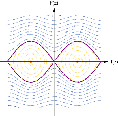
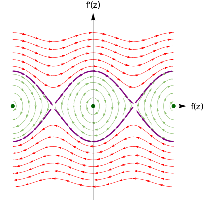
We call stationary solutions with waves speeds satisfying (respectively ) subluminal (superluminal). Representative phase portraits of subluminal and superluminal solutions to (5) are shown in Figure 1. Additionally, we call solutions whose orbits in phase space lie within the separatrix librational, and those whose orbits lie outside the separatrix rotational. This distinction is illustrated in Figure 1 in both the subluminal and superluminal cases. Librational waves correspond to For rotational waves, for subluminal waves and for superluminal waves.
Scott [28] was the first to study the stability of periodic traveling wave solutions to (1). He classified subluminal rotational waves as spectrally stable and determined spectral instability for all other types of waves, but these instability results were based on an incorrect claim that the spectrum in all cases was strictly confined to the real and imaginary axes. His proof has been corrected [18] and extended to the Klein-Gordon equation [19]. Using entirely different methods, we confirm the results in [18] and explicitly characterize all of parameter space. We also provide stability results for solutions perturbed by integer multiples of their fundamental period.
In Section 2 we present the elliptic solutions to (5) in Jacobi elliptic form from [18], and then reformulate the solutions into Weierstrass elliptic form. In Sections 3, 4 and 5, using the same methods as [6, 7, 13, 14], we exploit the integrability of (1) to associate the spectrum of the linear stability problem with the Lax spectrum using the squared eigenfunction connection [1]. This allows us to obtain an analytical expression for the spectrum of the operator associated with the linearization of (1) in the form of a condition on the real part of an integral over one period of some integrand. Similar to [14], we proceed by integrating the integrand explicitly in Section 6. Next, using the expressions obtained, we prove results concerning the location of the stability spectrum on the imaginary axis in Section 7. In Section 8, we present analytical results about the spectrum, and we make use of the integral condition to split parameter space into different regions where the spectrum shows qualitatively different behavior. Finally, in Section 9 we examine the spectral stability of solutions with respect to perturbations of an integer multiple of their fundamental period and prove various stability results.
2 Elliptic solutions
The derivation of the solutions is presented in the appendix of [18]. We limit our presentation to what is necessary for the following sections. For solutions to be real and nonsingular for real we require the following constraints:
| subluminal, | rotational: | (6) | ||||||
| superluminal, | rotational: | (7) | ||||||
| subluminal, | librational: | (8) | ||||||
| superluminal, | librational: | (9) |
Solutions to (5) are of the form
| (10) |
with the following parameter values for the various cases:
| subluminal, | rotational: | (11) | ||||||||||
| superluminal, | rotational: | (12) | ||||||||||
| subluminal, | librational: | (13) | ||||||||||
| superluminal, | librational: | (14) |
Here is the Jacobi elliptic function with elliptic modulus [9, 22, 34, 25]. We are neglecting to include a horizontal shift in . This additional parameter does not change the qualitative results and it is not included here.
Of some importance are the limits of these solutions on the boundaries of their regions of validity. On the boundaries for subluminal waves and superluminal waves the rotational and librational solutions limit to kink solutions. For subluminal waves that limit occurs when :
| (15) |
while for superluminal waves the limit is when :
| (16) |
These solutions are seen as the separatices in Figure 1 in purple and are on the purple curves in parameter space in Figure 2. The other limits for librational waves are when solutions limit to a constant. In the subluminal cases this occurs when and or in the superluminal case when and . For a general solution which is not on the boundary in parameter space, the solutions in (11-14) are periodic in with period where
| (17) |
the complete elliptic integral of the first kind.
We reformulate our elliptic solutions to (1) using Weierstrass elliptic functions [25] rather than Jacobi elliptic functions. This will simplify working with the integral condition (53) in Section 4, as formulas for integrating Weierstrass elliptic functions are well documented [9, 16]. It is important to note that nothing is lost by switching to Weierstrass elliptic functions, as we can map any Weierstrass elliptic function to a Jacobi elliptic function, and visa versa [25, 14]. Let
| (18) |
with and the lattice invariants of the Weierstrass function, , , and the zeros of the polynomial and and the half-periods of the Weierstrass lattice given by
| (19) |
| (20) |
Using (18) we convert our general solution in terms of Jacobi elliptic functions (10) to one in terms of Weierstrass elliptic functions:
| (21) |
with
| (22) |
| (23) |
| (24) |
| (25) |
where is the complement to given by . For all cases,
| (26) |
| (27) |
One motivation for using Weierstrass elliptic functions instead of Jacobi elliptic functions is that there is a unique expression for the lattice invariants and see (26-27) which holds for all cases, as opposed to Jacobi elliptic functions where a different elliptic modulus is used for each case see (11-14). The zeros of the polynomial are
| (28) |
These roots correspond to , , and where . For the various cases:
| subluminal, | rotational: | (29) | ||||||||
| superluminal, | rotational: | (30) | ||||||||
| subluminal, | librational: | (31) | ||||||||
| superluminal, | librational: | (32) |
3 The linear stability problem
To examine the linear stability of our solutions, we consider
| (33) |
where is a small parameter. Substituting (33) into (2), we obtain at order
| (34) |
Letting and we rewrite (34) as a first-order system of equations
| (35) |
An elliptic solution is linearly stable if for all there exists a such that if then for all . This definition depends on the choice of norm , which is specified in the definition of the spectrum in (38) below.
Since (35) is autonomous in , we separate variables to look for solutions of the form
| (36) |
resulting in the spectral problem
| (37) |
Here
| (38) |
or
| (39) |
For spectral stability, we need to demonstrate that the spectrum does not enter the open right half of the complex plane. Since (1) is Hamiltonian [3], the spectrum of its linearization is symmetric with respect to both the real and imaginary axis [35]. In other words, proving spectral stability for elliptic solutions to (1) amounts to proving that the stability spectrum lies strictly on the imaginary axis. We show that the elliptic solutions are spectrally stable only in the subluminal rotational case. We demonstrate spectral elements in the right-half plane near the origin for all choices of the parameters and outside the subluminal rotational regime.
4 The Lax problem
We wish to obtain an analytical representation for the spectrum . As mentioned in the introduction, this analytical representation comes from the squared eigenfunction connection between the linear stability problem (37) and the Lax pair of (1). The Lax pair for sine-Gordon is well known [2, 3, 1, 21]. The compatibility condition of the Lax pair,
| (40) |
| (41) |
is (1). We transform the Lax pair by moving into a traveling reference frame letting and Additionally, to examine the stationary solutions we let so that
| (42) |
| (43) |
where ∗ represents the complex conjugate, and
| (44) | ||||
| (45) | ||||
| (46) | ||||
| (47) |
whose compatibility condition is (4). We define , or informally the Lax spectrum, as the set of all for which (42) has a bounded (in z) solution. Examining (43), since and are independent of we separate variables. Let
| (48) |
with being independent of but possibly depending on . Substituting (48) into (43) and canceling the exponential, we find
| (49) |
To have nontrivial solutions, we require the determinant of (49) to be zero. Using the definitions of and , we get
| (50) |
As expected, is independent of both (by construction) and (by integrability). Thus is strictly a function of and the solution parameters and . We remark that takes the form (50) for all values of and regardless of where we are in parameter space.
To satisfy (49), we let
| (51) |
where is a scalar function. By construction of , satisfies (43). Since (42) and (43) commute, it is possible to choose such that also satisfies (42). Indeed, satisfies a first-order linear equation, whose solution is given by
| (52) |
For almost every , we have explicitly determined the two linearly independent solutions of (42), i.e., those corresponding to the positive and negative signs of in (50). Assuming these two solutions are, by construction linearly independent. In the case where is a root of the second solution to (42) can be determined via the reduction-of-order method.
Since (42) and (43) share eigenfunctions, is the set of all such that (51) is bounded for all . The vector part of is bounded for all , so we only need that the scalar function is bounded as . A necessary and sufficient condition for this is
| (53) |
where is the average over one period of the integrand, and Re denotes the real part. The integral condition (53) completely determines the Lax spectrum .
5 The squared eigenfunction connection
A connection between the eigenfunction of the Lax pair (42) and (43) and the eigenfunctions of the linear stability problem (37) using squared eigenfunctions is well known [1]. We prove the following theorem.
Theorem 5.1.
Proof.
The proof is done by direct calculation. Substitute into the left-hand side of (34). Eliminate -derivatives of and (up to order 2) using (42) and eliminate -derivatives of and (up to order 2) using (43). The resulting expression for the left-hand side is 0, thus demonstrating that (34) is satisfied, finishing the proof. ∎
To establish the connection between and we examine the right- and left-hand sides of (36). Substituting (54) and (48) to the left hand side of (36) we find
| (55) |
so we conclude that
| (56) |
with eigenfunctions given by
| (57) |
This gives the connection between the spectrum and the spectrum. It is also necessary to check that indeed all solutions of (37) are obtained through (55). This is not shown explicitly here, but is done analogous to the work in [6, 7].
Although in principle the above construction determines , it remains to be seen how practical this determination is. In the following section we discuss a technique for explicitly integrating (53) using Weierstrass elliptic functions, leading to a more explicit characterization of .
6 The Lax spectrum in terms of elliptic functions
In terms of Weierstrass elliptic functions, (53) becomes
| (58) |
with , , and given in (46-47). Substituting in for using (21) we find that (58) is
| (59) |
with with the dependence on , and suppressed. The ’s depend on but are independent of . Like , the ’s take one form regardless of where the solution is in parameter space. They are given by
| (60) | ||||
| (61) | ||||
| (62) | ||||
| (63) | ||||
| (64) |
We evaluate the integral in (59) explicitly [16]. We find
| (65) |
with
| (66) |
and is the Weierstrass Zeta function [25]. Note that is a multivalued function, but for our analysis is chosen as any value such that Substituting for the ’s (65) becomes
| (67) |
We simplify this further by recognizing that
| (68) |
Substituting in for and gives
| (69) |
Thus (67) simplifies to
| (70) |
where
| (71) |
Using (25), and applying the formula for the Weierstrass function evaluated at a half period [9], (70) becomes
| (72) |
Here
| (73) |
is the complete elliptic integral of the second kind. We have simplified the integral condition (58) significantly. Thus if and only if (72) is satisfied. To simplify notation, let
| (74) |
so that (72) is
| (75) |
Next, we wish to examine the level sets of the left-hand side of (75). To this end, we differentiate with respect to . To evaluate this derivative we use the chain rule and note that
| (76) |
Since
| (77) |
we use (69) to obtain
| (78) |
Taking the real part of (78) does not give another characterization of the spectrum. Instead, if we think of (72) as restricting to the zero level set of the left-hand side. Then we use (78) to determine a tangent vector field which allows us to map out level curves originating from any point. This is explained in more detail in Section 7.
7 The spectrum on the imaginary axis
In this section we discuss . As we demonstrate, this corresponds to the part of lying on the real axis for both rotational and librational waves, as well as a part of lying on the imaginary axis for rotational waves. Using (72) we obtain analytic expressions for corresponding to .
We begin by considering . As we demonstrate below, (72) is satisfied for any real . Using (50) and (56), we determine the corresponding parts of .
Theorem 7.1.
The condition (72) is satisified for .
Proof.
Since , , , and are real, it suffices to show that , , and . Rewriting (50) in the superluminal case,
| (79) |
and in the subluminal case,
| (80) |
In either case and . Since with takes real values to real values and purely imaginary values to purely imaginary values [25], to prove it suffices to show that For , maps to , and since we have that maps to . Thus we need to show that for , Again we split into cases. In the superluminal case, we want to show
| (81) |
Substituting in for using (79) and simplifying the left- and right-hand sides of this expression yields
| (82) |
Since , (82) is satisfied. For the subluminal case we proceed in a similar manner, noting the different value of from (29-32). We want to show
| (83) |
Substituting in for using (80) and simplifying the left- and right-hand sides of this expression yields
| (84) |
Since , (84) is satisfied. ∎
 |
 |
| (a) Subluminal: | (b) Superluminal: |
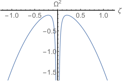
At this point, we know that . We wish to see what this corresponds to for . For convenience define
| (85) |
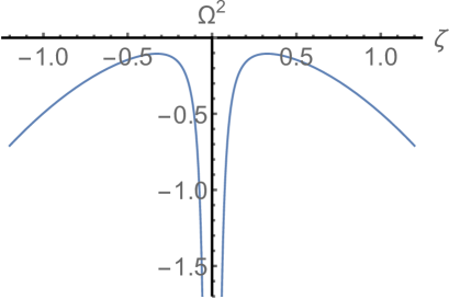
As was seen in the proof of Theorem 7.1, when , . Applying (56), we see that corresponds to . Representative plots of are shown in Figure 3. The subset of corresponding to consists of where is the maximum value of . The set corresponding to is quadruple covered as for all values of there are four values of which map to it, except at , where just two values of map to it. can be found explicitly by finding the extrema of . In the subluminal case, reaches its maxima at
| (86) |
and in the superluminal case, reaches its maxima at
| (87) |
Applying (56) we have where
| (88) |
in the subluminal case, and
| (89) |
in the superluminal case.
If satisfies , then must satisfy (72). This is due to the fact that the origin is always included in and hence in . The fact that there are four roots of corresponds to the fact that with multiplicity four. This is seen from the symmetries of (1) and by applying Noether’s Theorem [30, 20]. For rotational waves, the roots of lie on the imaginary axis. For the subluminal rotational case the roots are:
| (90) |
and in the superluminal rotational case the roots are:
| (91) |
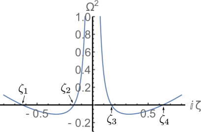
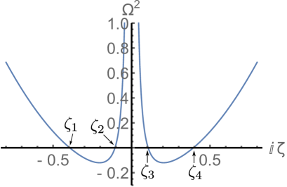
We label the four roots , , , and where They are labeled for reference in Figure 4.
Theorem 7.2.
For rotational waves, the condition (72) is satisified for all such that or .
Proof.
The level curve (75), is exactly the condition (72). We examine the tangent vector field to (75). If we let , then
| (92) |
Taking derivatives with respect to and gives a normal vector field to level curves of the general condition for any constant , specifically, the normal vector is given by
Thus, the tangent vector field is
By applying the chain rule and using we have that the tangent vector field to the level curves is
| (93) |
Where is given in (78). We note that the numerator of (78) is strictly real for , thus
| (94) |
Since for and for we have that
| (95) |
and thus on these intervals. Since at the endpoints , and (72) is satisfied. ∎
 |
 |
| (a) Subluminal: | (b) Superluminal: |
At this point we know that . We wish to see what this corresponds to for . Representative plots of , are shown in Figure 4. The subset of corresponding to consists of , where is the minimum value of . The set corresponding to is quadruple covered, except at the points , where the set is double-covered. can be found explicitly by finding the extrema of . In the subluminal rotational case, reaches its minima at
| (96) |
and in the superluminal rotational case, reaches its minima at
| (97) |
Applying (56) we have where
| (98) |
in the subluminal rotational case, and
| (99) |
in the superluminal rotational case.

8 Qualitatively different parts of the spectrum
Up to this point we have discussed only the subset of that is on the imaginary axis. In this section we discuss the rest of the spectrum. Except in the subluminal, rotational case, a part of is in the right-half plane (corresponding to unstable modes). For each of the other three regions we split parameter space into two subregions where is qualitatively different. Here is the closure of not on the imaginary axis.
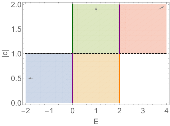
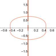
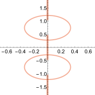
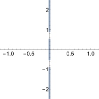
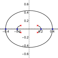
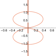
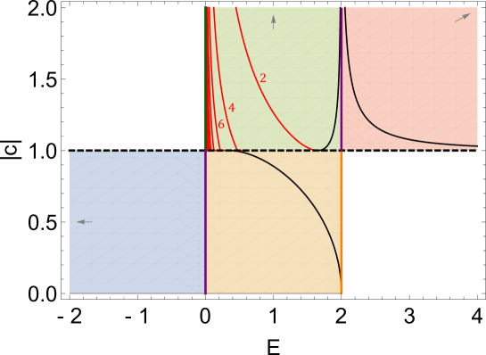
We refer to Figure 5, which shows parameter space with curves that split it into subregions where is qualitatively different. The exact curves splitting up the regions, and their derivations, are given below. In Figure 6 we show representative plots of for all qualitatively different spectra, and in Figure 7 we show the corresponding spectrum.
- •
-
•
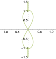
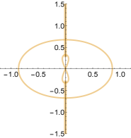
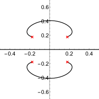
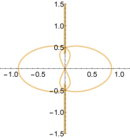
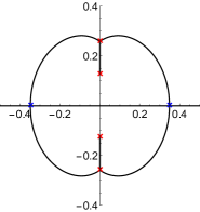
For the subluminal librational solutions, consists of either a double-covered infinity symbol, see Figure 6(f), or a double-covered figure 8 inset inside a double-covered ellipse-like curve, see Figure 6(g). The boundary between these regions is given explicitly below and a representative plot of on this boundary is seen in Figure 8(3a).
-
•
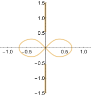
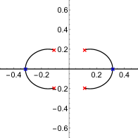
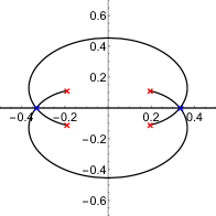
For the superluminal librational solutions, consists of either a double-covered figure 8, see Figure 6(a), or a double-covered infinity symbol inset inside a double-covered ellipse-like curve, see Figure 6(b). The boundary between these regions is given below and a representative plot of on this boundary is seen in Figure 8(1a).
-
•
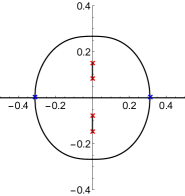
For the superluminal rotational solutions, consists of either a double-covered ellipse-like curve surrounding the origin, see Figure 6(c), or a double-covered ellipse-like curve in the upper- and lower-half plane, see Figure 6(d). The boundary between these regions is given explicitly below and a representative plot of on this boundary is seen in Figure 8(2a).
For all these cases, much can be proven and quantified explicitly, i.e., not in terms of special functions. Specifically, we calculate explicit expressions for and in the librational case we find explicit expressions for the tangents to around the origin. In fact, we are able to approximate the spectrum at the origin and around all points using a Taylor series to arbitrary order. These series give good approximations to the greatest real part of using only a few terms. They are not given in this paper, but follow from the same procedure as outlined in [14].
A method for determining is to take known points satisfying (72) and to follow the tangent vector field (93) from those points. We apply this technique from which we know to satisfy (72) from Theorem 7.1 as well as from the points satisfying .
8.1 Subluminal librational solutions
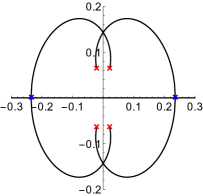
The roots of are given by
| (100) |
seen as red crosses in Figure 7(f,g). For convenience, we label these four roots where the subscript corresponds to the quadrant on the real and imaginary plane the root is in. In this case, (78) is
| (101) |
 |
 |
 |
 |
| (a) | (b) | (c) | (d) |
 |
 |
 |
| (e) | (f) | (g) |
Examining (93) for , for a vertical tangent in to occur, we need the numerator of (101) to be zero. Using the discriminant of as a function of we find the condition
| (102) |
for a vertical tangent to occur on the real axis. This condition is plotted as the black curve in the subluminal rotational region of Figure 5, and defines the split between qualitatively different spectra. Representative spectral plots for and on this boundary are seen in Figure 8(3). For solutions satisfying (102) we have the following
| (103) |
 |
 |
 |
 |
| (a) | (b) | (c) | (d) |
 |
 |
 |
| (e) | (f) | (g) |
and
| (104) |
shown as blue crosses in Figure 7(g). Mapping these points back to these points correspond to the top (or bottom) of the inset figure 8 in Figure 6(g):
| (105) |
and the ellipse-like curve in Figure 6(g):
| (106) |
 |
 |
 |
| (1a) | (2a) | (3a) |
 |
 |
 |
| (1b) | (2b) | (3b) |
Next we examine the slopes of at the origin. Because it suffices to examine the slopes for the set . We let and we consider as a function of so that . Applying the chain rule we have that the slope at any point in the set is
| (107) |
where
| (108) |
We examine (107) near where and . The slopes at the origin are
| (109) |
Further application of the chain rule can yield expressions for derivatives around the origin of any order, and the same technique can be applied around (105) and (106). In doing this we can obtain Taylor series approximations of to any order.
8.2 Superluminal librational solutions
The roots of are given by
| (110) |
seen as red crosses in Figure 7(f,g). As in Section 8.1, we label these four roots where the subscript corresponds to the quadrant on the real and imaginary plane the root is in. In this case, (78) is
| (111) |
Examining (93) for , for a vertical tangent in to occur, we need the numerator of (111) to be zero. In this case, there are always two real values of for which vertical tangents in occur:
| (112) |
shown as blue crosses in Figure 7(a,b). Mapping these points back to these points correspond to the top (or bottom) of the figure 8 in Figure 6(a) or the top (or bottom) of the ellipse-like curve in Figure 6(b):
| (113) |
In the subluminal librational case in Section 8.1, the qualitative change in the spectrum occurred when there was a bifurcation in the real values of with vertical tangents. In this case, there is no such bifurcation. The qualitative change in the spectrum occurs when there is a bifurcation in imaginary values of . The imaginary roots of the numerator of (111) are
| (114) |
The qualitative change occurs for and such that satisfies (72). This defines the curve seen in the superluminal librational region of Figure 5. Representative spectral plots for and on this boundary are seen in Figure 8(1). The slopes of at the origin are computed using the method described in Section 8.1. They are
| (115) |
As with the subluminal librational solutions, expressions for derivatives of any order around the origin and around (121) can be computed.
8.3 Superluminal rotational solutions
The roots of are given in (91), seen as red crosses in Figure 7(c,d). In this case, (78) is
| (116) |
Examining (93) for , for a vertical tangent in to occur, we need the numerator of (116) to be zero. In this case, again, there are always two real values of for which vertical tangents in occur:
| (117) |
shown as blue crosses in Figure 7(a,b). Mapping these points back to these points correspond to the top (or bottom) of the ellipse-like curve in Figure 6(c) and the top of the ellipse-like curve in the upper-half plane and the bottom of the ellipse-like curve in the lower-half plane in Figure 6(d):
| (118) |
As in the superluminal librational case above, we do not have a bifurcation in the real values of with vertical tangents. The qualitative change in the spectrum occurs when there is a bifurcation in imaginary values of . The imaginary roots of the numerator of (116) are
| (119) |
The qualitative change occurs for and such that and where and are the smallest and largest roots of respectively. This condition is seen in Figure 8(2b) and is
| (120) |
For , we map to and find these points corresponding to the bottom of the ellipse-like curve in the upper-half plane and the top of the ellipse-like curve in the lower-half plane in Figure 6(d):
| (121) |
9 Floquet theory and subharmonic perturbations
We examine using a Floquet parameter description. We use this to prove spectral stability results with respect to perturbations of an integer multiple of the fundamental period of the solution, i.e., subharmonic perturbations.
We write the eigenfunctions from (37) using a Floquet-Bloch decomposition
| (122) |
with [12, 14]. Here for all solutions. From Floquet’s Theorem [12], all bounded solutions of (37) are of this form, and our analysis includes perturbations of an arbitrary period. Specifically, for corresponds to perturbations of the same period of the solutions, and in general
| (123) |
corresponds to perturbations of period . The choice of the specific range of is arbitrary as long as it is of length . For added clarity in this section, we plot figures using the larger ranges , periodically extending beyond the basic region.
In the previous sections is parameterized in terms of . We wish to re-parameterize in terms of . We examine the eigenfunction from (122). From the periodicity of we have
| (124) |
Using (57), (51), and (52), we find
| (125) |
where we have used the periodicity properties
| (126) |
Using (72),
| (127) |
where is given in (74) and .
In what follows we discuss the stability of solutions with respect to perturbations of integer multiples of their fundamental periods, so-called subharmonic perturbations [17]. The expression (127) gives an easy way to do this. Specifically, from (123) we know which values of correspond to perturbations of what type. For stability with respect to perturbations of period , we need all spectral elements associated with a given value to have zero real part. In Figure 9 we plot the real part of as a function of using (50), (56), and (127). We rescale by for consistency in our figures. Here
| (128) |
corresponds to perturbations of for any integer .
The following results are obtained in each region of parameter space:
- •
-
•
For the subluminal librational case, all solutions are spectrally unstable with respect to all subharmonic perturbations. This is shown in Section 9.1.
-
•
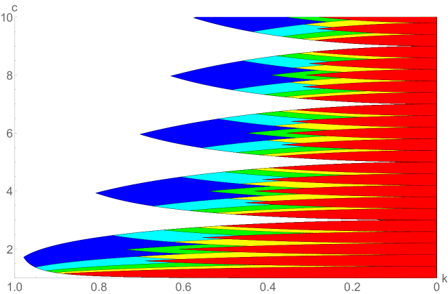
For the superluminal librational case, all solutions are spectrally unstable, but all solutions left of curve 2 in Figure 10 are stable with respect to perturbations of twice the period and the same period, all solutions left of curve 4 are stable with respect to perturbations of four times the period, all solutions left of curve 6 are stable with respect to perturbations of six times the period, as well as three times the period, etc. This is shown in Section 9.2.
- •
 |
 |
 |
 |
| (a) | (b) | (c) | (d) |
 |
 |
 |
 |
| (e) | (f) | (g) | (h) |
We provide the following useful lemma:
Lemma 9.1.
For any analytic function on a contour where constant, is strictly monotone, provided the contour does not traverse a saddle point. Similarly, on a contour where constant, is strictly monotone, provided the contour does not traverse a saddle point.
Proof.
This is an immediate consequence of the Cauchy-Riemann relations [5]. ∎
Thus along contours where if there are no saddle points, then is monotone. If we fix and , using (127) we see that is also monotone along curves with . In what follows, we omit .
9.1 Subluminal librational solutions
There are two cases to consider for subluminal librational solutions, corresponding to the two qualitatively different stability spectra seen in Figure 6(f,g), and their corresponding Lax spectra in Figure 7(f,g). Representative plots of vs. for these cases are shown in Figure 9(a,b). We prove the following theorem:
Theorem 9.2.
The subluminal librational solutions to (1) are unstable with respect to all subharmonic perturbations.
Proof.
It suffices to show that for some , and . We split into cases with qualitatively different spectra:
-
1.
In the case where the stability spectrum looks qualitatively like an infinity symbol, we examine , see Figure 7(f). The infinity symbol spectrum is double covered, so without loss of generality, we consider only values of in the upper-half plane. Specifically, we consider values of ranging from to , moving from the red cross in the second quadrant to the red cross in the first quadrant of Figure 7(f). At , and . As moves from to , monotonically increases (Lemma 9.1) until it reaches at , where , see Figure 9(a). Along this curve so by the intermediate value theorem at some point between and , with .
-
2.
In the case where the stability spectrum looks qualitatively like a figure 8 inset in an ellipse-like curve, examine , see Figure 7(g). The spectrum has two components, corresponding to the figure 8, and corresponding to the ellipse-like curve. For instability, we only need to examine corresponding to the ellipse-like curve. Again, we consider only values of in the upper-half plane. Specifically, we consider values of ranging from to , moving from the blue cross in the second quadrant to the blue cross in the first quadrant of Figure 7(g). At , , and . As moves from to , monotonically increases (Lemma 9.1) until it reaches at , with , see the ellipse-like curve in Figure 9(b). Because of the symmetries of for we have that . Along this curve so again by the intermediate value theorem at some point between and , with .
∎
9.2 Superluminal librational solutions
Theorem 9.3.
The superluminal librational solutions to (1) are stable with respect to subharmonic perturbations of period if they satisfy the condition
| (129) |
for odd, and
| (130) |
for even.
Proof.
For stability with respect to perturbations of period we need that for , the spectral elements have zero real part, i.e., for .
We examine , in the figure 8 case, see Figure 7(a). The figure 8 spectrum is double covered, so, without loss of generality, we consider only values of in the left-half plane. Specifically we consider values of ranging from to passing along the level curve through . At , and . As moves from to , monotonically decreases (Lemma 9.1) until it reaches at . At , . Note that we are only considering the lower-left quarter plane. The analysis for ranging from to is symmetric in .
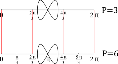
Qualitatively, we have figure 8s centered at and extending over , see Figure 9(c,d). Relevant to the interval is the figure 8 centered at . For stability, we need the left-most edge of the figure 8 to be to the right of for odd and to the right of for even. Similarly, we need the right-most edge of the figure 8 to be to the left of for odd and to the left of for even. These conditions are for odd:
| (131) |
and for even:
| (132) |
These conditions simplify to give (129) and (130) respectively. ∎
 |
 |
||
| (a) Superluminal librational | (b) Superluminal rotational |
We remark that for a given odd the condition (129) is the same as the condition (130) for . Thus, for superluminal librational waves if we have stability with respect to perturbations of some odd multiple of the period we also have stability with respect to perturbations of . This is shown in the case when in Figure 11(a). These results are summarized in Figure 10 where we plot only the condition (130). We remark that it is possible for solutions to be stable with respect to perturbations of four times the period but not with respect to three times the period. Solutions of this type would lie to the left of curve 4 but to the right of curve 6 in Figure 10. More generally it is possible to have solutions which are stable with respect to times the period but not with respect to times the period where is even and less than .
9.3 Superluminal rotational solutions
Theorem 9.4.
The superluminal rotational solutions to (1) are stable with respect to subharmonic perturbations of period if they simultaneously satisfy the conditions
| (133) |
| (134) |
for some and some . Note that and .
Proof.
For stability with respect to perturbations of period we need that for , the spectral elements have zero real part for all .
We examine , in the case where we have ellipse-like curves in the upper- and lower-half planes, see Figure 7(d). As in Theorem 9.3, using symmetries we restrict ourselves to in the upper-left quarter plane. Specifically we consider values of ranging from to . At , and . As moves from to , monotonically decreases (Lemma 9.1) until it reaches at . At , .
Qualitatively, we have an ellipse-like curve beginning at and extending to , see Figure 9(g,h). The only values of with lie within the range So if , for some , then for for all .
These results are summarized in Figure 12. We choose to rescale parameter space using the elliptic modulus , to show the extent of the subharmonic stability regions as . We only show regions for for the sake of clarity.
We see that there are many disjoint regions of subharmonic stability for each value of corresponding to the various choices for . Within each disjoint region of stability for same period perturbations (blue) there are disjoint regions of stability with respect to perturbations of times the period. This follows directly from the conditions (133) and (134).
We note the possibility of solutions which are stable with respect to three times the period of the solution but not with respect to two times the period of the solution. An example of what looks like in this case is shown in Figure 9(h) with Indeed it is possible to have solutions which are stable with respect to times the period of the solution but not with respect to times the period of the solution for any where . From Figure 12 we notice that if a solution is stable with respect to perturbations of five times the period (red) it is stable with respect to either perturbations of two times the period (light blue) or three times the period (green). This is proved by a simple topological argument shown in Figure 11(b) and explained in the caption.
10 Conclusion
In this paper, the methods of [14] are used to examine and explicitly determine the stability spectrum of the stationary solutions of the sine-Gordon equation. As in [14], we demonstrate that the parameter space for the stationary solution separates in different regions where the topology of the spectrum is different. An additional subdivision of this parameter space is found for superluminal waves when considering the stability of the solutions with respect to subharmonic perturbations of a specific period. We find solutions which are stable with respect to perturbations of times the period but unstable with respect to times the period, where .
11 Acknowledgments
This work was supported by the National Science Foundation through grant NSF-DMS-100801 (BD). Benjamin L. Segal acknowledges funding from a Department of Applied Mathematics Boeing fellowship and the Achievement Rewards for College Scientists (ARCS) fellowship. Any opinions, findings, and conclusions or recommendations expressed in this material are those of the authors and do not necessarily reflect the views of the funding sources.
References
- [1] Ablowitz, M. J., Kaup, D. J., and Newell, A. C. The inverse scattering transform-Fourier analysis for nonlinear problems. Studies in Applied Mathematics 53 (1974), 249–315.
- [2] Ablowitz, M. J., Kaup, D. J., Newell, A. C., and Segur, H. Method for solving the sine-Gordon equation. Phys. Rev. Lett. 30 (1973), 1262–1264.
- [3] Ablowitz, M. J., and Segur, H. Solitons and the inverse scattering transform, vol. 4. Society for Industrial and Applied Mathematics (SIAM), Philadelphia, 1981.
- [4] Barone, A., Esposito, F., Magee, C. J., and Scott, A. C. Theory and applications of the sine-Gordon equation. La Rivista del Nuovo Cimento 1, 2 (1971), 227–267.
- [5] Born, M., and Wolf, E. Principles of optics: Electromagnetic theory of propagation, interference and diffraction of light. Pergamon Press, New York, 1959.
- [6] Bottman, N., and Deconinck, B. KdV cnoidal waves are spectrally stable. Discrete and Continuous Dynamical Systems-Series A (DCDS-A) 25 (2009), 1163–1180.
- [7] Bottman, N., Deconinck, B., and Nivala, M. Elliptic solutions of the defocusing NLS equation are stable. Journal of Physics A: Mathematical and Theoretical 44 (2011), 285201.
- [8] Bour, E. M. Théorie de la déformation des surfaces. Journal de L’école Impériale Polytechnique 22 (1862), 1–148.
- [9] Byrd, P. F., and Friedman, M. D. Handbook of elliptic integrals for engineers and physicists. Springer-Verlag, Berlin, 1954.
- [10] Coleman, S. Quantum sine-gordon equation as the massive Thirring model. Phys. Rev. D 11 (1975), 2088–2097.
- [11] Dauxois, T., and Peyrard, M. Physics of solitons. Cambridge University Press, Cambridge, 2006.
- [12] Deconinck, B., and Kapitula, T. The orbital stability of the cnoidal waves of the Korteweg–de Vries equation. Physics Letters A 374 (2010), 4018–4022.
- [13] Deconinck, B., and Nivala, M. The stability analysis of the periodic traveling wave solutions of the mKdV equation. Stud. Appl. Math. 126, 1 (2011), 17–48.
- [14] Deconinck, B., and Segal, B. L. The stability spectrum for elliptic solutions to the focusing NLS equation. Physica D: Nonlinear Phenomena 346 (2017), 1–19.
- [15] Frenkel, J., and Kontorova, T. On the theory of plastic deformation and twinning. Acad. Sci. U.S.S.R. J. Phys. 1 (1939), 137–149.
- [16] Gradshteyn, I. S., and Ryzhik, I. M. Table of integrals, series, and products, eighth ed. Elsevier/Academic Press, Amsterdam, 2015.
- [17] Gustafson, S., Le Coz, S., and Tsai, T.-P. Stability of periodic waves of 1D cubic nonlinear Schrödinger equations. arXiv:1606.04215.
- [18] Jones, C. K., Marangell, R., Miller, P. D., and Plaza, R. G. On the stability analysis of periodic sine–Gordon traveling waves. Physica D: Nonlinear Phenomena 251 (2013), 63–74.
- [19] Jones, C. K. R. T., Marangell, R., Miller, P. D., and Plaza, R. G. Spectral and modulational stability of periodic wavetrains for the nonlinear Klein-Gordon equation. J. Differential Equations 257, 12 (2014), 4632–4703.
- [20] Kapitula, T., and Promislow, K. Spectral and dynamical stability of nonlinear waves, vol. 185. Springer, New York, 2013.
- [21] Kaup, D. J. Method for solving the sine-Gordon equation in laboratory coordinates. Studies in Appl. Math. 54, 2 (1975), 165–179.
- [22] Lawden, D. F. Elliptic functions and applications, vol. 80. Springer-Verlag, New York, 1989.
- [23] Liang, E. Nonlinear periodic waves in a self-gravitating fluid and galaxy formation. The Astrophysical Journal 230 (1979), 325–329.
- [24] Newell, A. C. Solitons in mathematics and physics, vol. 48 of CBMS-NSF Regional Conference Series in Applied Mathematics. Society for Industrial and Applied Mathematics (SIAM), Philadelphia, PA, 1985.
- [25] Olver, F., Ed. NIST handbook of mathematical functions. Cambridge University Press, New York, 2010.
- [26] Remoissenet, M. Waves called solitons: concepts and experiments. Springer-Verlag, Berlin, 1994.
- [27] Scott, A. C. A nonlinear Klein-Gordon equation. American Journal of Physics 37, 1 (1969), 52–61.
- [28] Scott, A. C. Waveform stability on a nonlinear Klein-Gordon equation. Proceedings of the IEEE 57, 7 (1969), 1338–1339.
- [29] Scott, A. C. Propagation of magnetic flux on a long Josephson tunnel junction. Il Nuovo Cimento B 69, 2 (1970), 241–261.
- [30] Sulem, C., and Sulem, P.-L. The nonlinear Schrödinger equation: Self-focusing and wave collapse, vol. 139. Springer-Verlag, New York, 1999.
- [31] Voglis, N. Solitons and breathers from the third integral of motion in galaxies. Monthly Notices of the Royal Astronomical Society 344, 2 (2003), 575–582.
- [32] Voglis, N., Tsoutsis, P., and Efthymiopoulos, C. Invariant manifolds, phase correlations of chaotic orbits and the spiral structure of galaxies. Monthly Notices of the Royal Astronomical Society 373, 1 (2006), 280–294.
- [33] Waldram, J., Pippard, A., and Clarke, J. Theory of the current–voltage characteristics of SNS junctions and other superconducting weak links. Phil. Trans. Roy. Soc. London, Ser. A 268: 265-87 (1970).
- [34] Whittaker, E. T., and Watson, G. N. A course of modern analysis. An introduction to the general theory of infinite processes and of analytic functions: with an account of the principal transcendental functions. Cambridge University Press, New York, 1962.
- [35] Wiggins, S. Introduction to applied nonlinear dynamical systems and chaos, second ed., vol. 2. Springer-Verlag, New York, 2003.
- [36] Yakushevich, L. V. Nonlinear physics of DNA. John Wiley & Sons, Weinheim, 2006.