Incentivizing Reliable Demand Response with Customers’ Uncertainties and Capacity Planning

1. Introduction

One of the major issues with the integration of renewable energy sources into the power grid is the increased uncertainty and variability that they bring. If this uncertainty is not sufficiently addressed, it will limit the further penetration of renewables into the grid and even result in blackouts. Compared to energy storage, Demand Response (DR) has advantages to provide reserves to the load serving entities (LSEs) in a cost-effective and environmentally friendly way. DR programs work by changing customers’ loads when the power grid experiences a contingency such as a mismatch between supply and demand. Uncertainties from both the customer-side and LSE-side make designing algorithms for DR a major challenge.

This paper makes the following main contributions: (i) We propose DR control policies based on the optimal structures of the offline solution. (ii) A distributed algorithm is developed for implementing the control policies without efficiency loss. (iii) We further offer an enhanced policy design by allowing flexibilities into the commitment level. (iv) We perform real world trace based numerical simulations which demonstrate that the proposed algorithms can achieve near optimal social cost. Details can be found in our extended version (Comden et al., 2017).

2. Optimization Problem

The goal is to simultaneously decide the capacity planning $\kappa$ and a practical DR policy $\mathbf{x}(D,\boldsymbol{\delta})$ to minimize the expected social cost caused by a random aggregate supply-demand mismatch $D$ (which captures mismatches from both the generation side and the load side).

$$\min_{\kappa,\mathbf{x}(D,\boldsymbol{\delta})} C_{\text{cap}}(\kappa)$$

$$+\mathbb{E}_{D,\boldsymbol{\delta},\mathbf{C}(\cdot)}\left[\sum_{i}C_{i}(x_{i}(D,\delta_{i}))+C_{\text{g}}\left(D-\sum_{i}x_{i}(D,\delta_{i})\right)\right]$$

(1a) s.t. $$\max_{D,\boldsymbol{\delta}}\left\{D-\sum_{i}x_{i}(D,\delta_{i})\right\}\leq\kappa$$

(1b) $$\min_{D,\boldsymbol{\delta}}\left\{D-\sum_{i}x_{i}(D,\delta_{i})\right\}\geq-\kappa.$$

where $\delta_{i}$ and $C_{i}(\cdot)$ are respectively for customer $i$ the individual random demand mismatch and random cost function (e.g. $a_{i}x_{i}^{2}$ with $a_{i}$ as a random coefficient) for performing DR, $C_{\text{cap}}(\cdot)$ and $C_{\text{g}}(\cdot)$ are respectively the LSE’s cost for purchasing capacity and for managing the remaining mismatch, We note that (1a) and (1b) are worst-case constraints so that the remaining mismatch does not go beyond the purchased capacity. The two main challenges of this problem are (i) deciding the optimal capacity $\kappa$ before implementing the DR policy, and (ii) optimizing an online DR policy. The cost functions are assumed to be convex.

Optimal Real-time Solution

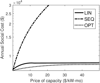
(a) LIN

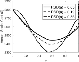
(b) LIN${}^{+}(\rho)$

Figure 1. Annual Social Cost vs. (a) price of capacity in LIN compared to different baselines, (b) level of commitment in LIN${}^{+}(\rho)$ for different amounts of Relative Standard Deviations (RSD) on the customer cost parameter $a$.

We provide the characterization of the optimal real-time solution to reveal special structures that we take advantage of in our policy design (Section 3). The real-time DR decision problem for a given capacity $\kappa$ at a time $t$ is:

(2a) $$R(\kappa;t):=\min_{\mathbf{x}(t)}\quad \sum_{i}C_{i}(x_{i}(t);t)+C_{\text{g}}\left(D(t)-\sum_{i}x_{i}(t)\right)$$

(2b) s.t. $$-\kappa\leq D(t)-\sum_{i}x_{i}(t)\leq\kappa.$$

Lemma 2.1.

Problem (2) is a convex optimization problem.

The Karush-Kuhn-Tucker (KKT) optimality conditions of this real-time problem show that when the capacity constraint on $\kappa$ is non-binding, i.e., $-\kappa<D(t)-\sum_{j\in\mathcal{V}}x_{j}^{*}(t)<\kappa$, it implies that $C^{\prime}_{i}(x_{i}^{*}(t))=C^{\prime}_{\text{g}}(D(t)-\sum_{j\in\mathcal{V}}x_{j}^{*}(t))$. This means that the marginal cost for each customer to provide demand response is the same, all of which is equal to the LSE’s marginal cost to tolerate the mismatch. Furthermore, we get the following lemma which helps determine the optimal capacity in the next subsection:

Lemma 2.2.

$R(\kappa;t)$ as defined by (2) is a convex function of $\kappa$. Additionally the negative of the sum of dual variables $\underline{\theta}+\overline{\theta}$ from constraint (2b) is the subgradient of $R(\kappa;t)$ w.r.t. $\kappa$.

Optimal Capacity

We can use the real-time decision problem (2) to decide what the optimal capacity should be in the following capacity problem:

(3) $$\min_{\kappa}\quad C_{\text{cap}}(\kappa)+\mathbb{E}_{D,\boldsymbol{\delta},\mathbf{C}(\cdot)}\left[R(\kappa;t)\right]$$

Theorem 2.3.

(3) is a convex optimization problem over $\kappa$.

The KKT optimality conditions for the capacity problem and Lemma 2.2 give us the following result:

(4) $$C^{\prime}_{\text{cap}}(\kappa^{*})=\mathbb{E}_{D,\boldsymbol{\delta},\mathbf{C}(\cdot)}\left[\theta(\kappa^{*};t)\right]$$

where we use the notation of $\theta(\kappa;t)$ as a function to represent the sum of the optimal dual variables for constraint (2b). This means that for an optimal capacity, the marginal cost of capacity must equal the expected dual price for that capacity constraint.

3. Policy Design

Linear policy

Motivated by the desire to find a simple DR policy $\mathbf{x}(D,\delta_{i\in\mathcal{V}})$ that preserves convexity, we focus on a simple but powerful linear demand response policy that is a function of total and local net demands:

(5) $$x_{i}(D,{\delta}_{i})=\alpha_{i}D+\beta_{i}{\delta}_{i}+\gamma_{i}.$$

Intuitively, there are three components: $\alpha_{i}D$ implies each customer shares some (predefined) fraction of the global mismatch $D$; $\beta_{i}{\delta}_{i}$ means customer $i$ may need to take additional responsibility for the mismatch due to his own demand fluctuation and estimation error; finally, $\gamma_{i}$, the constant part, can help when the random variables $\mathbb{E}[D]$ and/or $\mathbb{E}[\delta_{i}]$ is nonzero. Then the LSE needs to solve (1) with (5) to obtain the optimal parameters for the linear contract, i.e., $\boldsymbol{\alpha},\boldsymbol{\beta},\boldsymbol{\gamma}$, as well as the optimal capacity $\kappa$.

Theorem 3.1.

Problem (1) with the linear policy (5) is a convex optimization problem.

Distributed algorithm

In most cases, the LSE’s information on the customers’ cost functions is much less accurate than the customer themselves’. This can also be due to privacy concerns. To handle this, we design a distributed algorithm so that the LSE does not need the information of the customer cost functions, while still achieving the optimal $(\kappa^{LIN},\boldsymbol{\alpha}^{*},\boldsymbol{\beta}^{*},\boldsymbol{\gamma}^{*})$ for Problem (1) with the linear policy (5). We introduce and substitute $(u_{i},v_{i},w_{i})$ for $(\alpha_{i},\beta_{i},\gamma_{i})$ in each customer’s estimated cost function $\hat{C}_{i}(\cdot)$ and the LSE uses the corresponding price set $(\pi_{i},\lambda_{i},\mu_{i})$ to incentivize each customer to change their parameters.

Distributed Algorithm for LIN: (0) Initialization: $(\boldsymbol{\alpha},\boldsymbol{\beta},\boldsymbol{\gamma},\mathbf{u},\mathbf{v},\mathbf{w},\boldsymbol{\pi},\boldsymbol{\lambda},\boldsymbol{\mu}):=\mathbf{0}$. (1) LSE: receives $(u_{i},v_{i},w_{i})$ from each customer $i\in\mathcal{V}$. • Solves Problem (9) and updates $(\boldsymbol{\alpha},\boldsymbol{\beta},\boldsymbol{\gamma})$ with the optimal solution. • Updates the stepsize: (6) $$\eta=\frac{\zeta/k}{||(\boldsymbol{\alpha},\boldsymbol{\beta},\boldsymbol{\gamma})-(\mathbf{u},\mathbf{v},\mathbf{w})||_{2}}$$ where $\zeta$ is a small constant and $k$ is the iteration number. • Updates the dual prices, $\forall i\in\mathcal{V}$: (7) $$(\pi_{i},\lambda_{i},\mu_{i}):=(\pi_{i},\lambda_{i},\mu_{i})+\eta\left((\alpha_{i},\beta_{i},\gamma_{i})-(u_{i},v_{i},w_{i})\right)$$ • Sends $(\pi_{i},\lambda_{i},\mu_{i})$ to the each customer respectively. (2) Customer $i\in\mathcal{V}$: receives $(\pi_{i},\lambda_{i},\mu_{i})$ from LSE. • Solves Problem (8) and updates $(u_{i},v_{i},w_{i})$ with optimal solution. • Sends $(u_{i},v_{i},w_{i})$ to the LSE. (3) Repeat Steps 1-2 until $||(\boldsymbol{\alpha},\boldsymbol{\beta},\boldsymbol{\gamma})-(\mathbf{u},\mathbf{v},\mathbf{w})||_{2}\leq\epsilon$ where $\epsilon$ is the tolerance on magnitude of the subgradient.

Thus $\pi_{i}u_{i}+\lambda_{i}v_{i}+\mu_{i}w_{i}$ is the total payment to customer $i$ for the linear demand response policy. The individual customer’s problem for a given set of prices is

(8) $$\min_{u_{i},v_{i},w_{i}}\mathbb{E}_{D,\delta_{i}}\left[\hat{C}_{i}(u_{i}D+v_{i}{\delta}_{i}+w_{i})\right]-\pi_{i}u_{i}-\lambda_{i}v_{i}-\mu_{i}w_{i}$$

while the LSE’s optimization problem among all the customers is

$$\min_{\boldsymbol{\alpha},\boldsymbol{\beta},\boldsymbol{\gamma},\kappa}\text{ } C_{\text{cap}}\left(\kappa\right)+\sum_{i\in\mathcal{V}}(\pi_{i}\alpha_{i}+\lambda_{i}\beta_{i}+\mu_{i}\gamma_{i})$$

(9) $$\quad+\mathbb{E}_{D,\boldsymbol{\delta}}\left[C_{\text{g}}\left(\sum_{i\in\mathcal{V}}({\delta}_{i}-\alpha_{i}D-\beta_{i}{\delta}_{i}-\gamma_{i})-r\right)\right]$$

s.t. $$\eqref{const:CAPpolicy1},\eqref{const:CAPpolicy2}$$

In order for the customers and the LSE to negotiate and obtain the optimal prices we use the Subgradient Method (see (Bertsekas, 1999) Chapter 6).

Theorem 3.2.

The distributed algorithm’s trajectory of dual prices converge to the optimal dual prices for Problem (1) with (5).

Flexible Commitment Demand Response

One potential drawback of LIN is that customers are forced to follow the specified linear policy. In some cases, customers may face a very high cost to follow the policy, e.g., when there are some critical jobs to be finished, represented by a larger $a_{i}(t)$. Motivated by this observation and some existing regulation service programs, we modify the LIN policy to add some flexibility limited by a single parameter $\rho$. We call the new algorithm LIN${}^{+}(\rho)$ where each customer has up to $1-\rho$ (in percentage) of the time slots in which they do not need to follow the policy according to her realized $\alpha_{i}(t)$. In other words, she may let $x_{i}(t)=0$ for such timeslots. Note that although we add the flexibility to LIN in this paper, the approach is in fact general and can be applied to a wide range of fully committed programs.

4. Performance Evaluation

Experimental Setup

We simulate an LSE supplying power to 300 customers. Each customer has a particular demand of load which we model by utilizing the traces obtained from the UMass Trace Repository (Barker et al., 2012).

LIN is close to optimal

Figure 1(a) compares the social cost of LIN to baselines using the offline optimal OPT (3) as a lower bound and sequential algorithm SEQ as an upper bound. The baseline SEQ first makes a conservative capacity planning decision about $\kappa$, and then sets a price for DR to obtain a targeted amount of DR. The social cost of LIN is no more than $10\%$ higher compared to the fundamental limit OPT and is significantly less than SEQ. The social cost of SEQ increases rapidly with increasing capacity prices because of the conservative 90kW capacity used by SEQ to protect the system from any leftover mismatch.

Additional cost savings brought by LIN${}^{+}(\rho)$

Depicted in Figure 1(b), as $\rho$ decreases from 1, the social cost first decreases due to the fact that some customers with very high $a_{i}(t)$ are allowed to not provide demand response. As $\rho$ continues to decrease, we have more customers not providing demand response and the cost actually goes up again. This is because the LSE’s penalty for the mismatch becomes larger than the costs of customers to provide demand response. At $\rho=0.8$, it achieves a cost savings 7-8%. Recall that the gap between LIN and the offline optimal OPT is about 10%. This means LIN${}^{+}(\rho^{*})$ achieves near optimal cost.

5. Acknowledgments

This research is supported by NSF grants CNS-1464388 and CNS-1617698.

References

- (1)
- Barker et al. (2012) Sean Barker, Aditya Mishra, David Irwin, Emmanuel Cecchet, Prashant Shenoy, and Jeannie Albrecht. 2012. Smart*: An open data set and tools for enabling research in sustainable homes. SustKDD, August 111 (2012), 112.
- Bertsekas (1999) Dimitri P Bertsekas. 1999. Nonlinear programming. Athena scientific Belmont.
- Comden et al. (2017) Joshua Comden, Zhenhua Liu, and Yue Zhao. 2017. Harnessing Flexible and Reliable Demand Response Under Customer Uncertainties. arXiv preprint arXiv:1704.04537 (2017).