Electromagnetic modes from Stoner enhancement

Abstract

Systems with substantial spin fluctuations, can internally dress the polarization function by ladder diagram of Stoner (spin-flip) excitations. This process can drastically modify the electromagnetic response. As a case study we provide detailed analysis of the corrections to the non-local optical conductivity of both doped and undoped graphene. While the resummation of ladder diagram of Stoner excitations does not affect the TE mode in doped graphene, it allows for a new undampled TM mode in undoped graphene. This is the sole effect of corrections arising from ladder diagrams and is dominated by Stoner excitations along the ladder rung which goes away by turning off the source of spin-flip interactions.

url]http://physics.sharif.edu/ jafari/

1 Introduction

Spin fluctuations are considered to be important players in strongly correlated systems and their associated magnetic properties [1]. These sort of fluctuations are among the possible scenarios for the explanation of Cooper pairing in strongly correlated systems, including the recent Iron based superconductors [2]. Placing a material with strong spin fluctuations such as a spin ice in proximity to a metallic layer has been proposed as a mechanism to customize the electron-electron interaction [3]. In itinerant systems all one needs is a strong enough source of spin fluctuations. This source is nothing but the short range interaction called the Hubbard $U$ which prohibits simultaneous presence of two electrons at the same orbital by billing a high enough cost for double occupancy as $Un_{i\uparrow}n_{i\downarrow}$. Here $i$ refers to an atomic orbital localized in a given site $i$ and $n=c^{\dagger}c$ is the fermionic occupation number. To see why the short range part of Coulomb interaction can so efficiently generate spin flip, simply rewrite $Uc^{\dagger}_{1\uparrow}c^{\dagger}_{2\downarrow}c_{3\downarrow}c_{4\uparrow}$ where $1\ldots 4$ are appropriate momentum indices as $-Uc^{\dagger}_{1\uparrow}c^{\dagger}_{2\downarrow}c_{4\uparrow}c_{3\downarrow}$. The later form can be interpreted as attraction in the spin-flip or Stoner channel. This is how short-ranged Coulomb interactions can lead to spin-flip processes and cause spin-flip particle-hole (PH) fluctuations.

How do the spin fluctuations of materials manifest in the propagation of electromagnetic (EM) modes? Put it differently, is there a optical or EM way of directly probing the spin-fluctuations? The EM response of any system is determined by a fermion bubble to which two external photon propagators are attached (Fig. 1a). The bubble itself can be internally dressed via the so called ladder diagrams (Fig. 1b). The popular approximation known as random phase approximation amounts to ignoring all the ladder diagrams. This is equivalent to keeping only the first (empty bubble) diagram in Fig. 1b. However, if the materials properties are such that the Hubbard $U$ is strong enough to generate strong spin-fluctuations of the type described above, it is important to encode them into appropriate ladder daigram resummation. This is is well-known in the context of high temperature superconductors [4]. Once a PH pair is created by a light beam, the Hubbard $U$ takes care of the spin flips across the rung of the ladder. Before the PH pairs recombine to emit back a the photon, a resonance enhancement of spin-flip processes known as Stoner enhancement can give rise to a singularity in the response to the EM radiation. This effect as we will show in great detail in present work, drastically modifies the propagation of EM radition in systems that host strong spin fluctuations. When a Hubbard vertex is inserted on the way of a PH pair running across the rungs of a ladder, irrespective of whether the spin is flipped or not, it generates a fluctuation of the very same electric charge, and hence is expected to quite directly affect the dielectric properties. The essential difference between the spin-flip and non-spin-filp ladder diagrams will be the sign $\pm U$ of the basic interaction vertex.

a)

b)

(

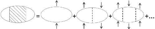
(a)

(

(b)

Figure 1: (a) General polarization function that determines coupling of any system with external photons. (b) Ladder diagrams corresponding to Stoner (spin-flip) excitations across the rung. Note that for particle-hole bubbles, particle and hole run in opposite directions along the rung. Keeping only the first term in the right hand side corresponds to the commonly used random-phase approximation.

Is there a simple platform that allows for interesting EM properties, and at the same time hosts strong enough fluctuations of spins? One of the exciting materials of the past decade has been the two-dimensional graphene which has attracted great deal of attention during recent years. This mono layer material consists of carbon atoms which are arranged in honeycomb lattice and the energy spectrum of this material consists of two Dirac cones in the Brillouin zone where conduction and valence bands linearly touch each other [5, 6, 7]. Intrinsic graphene is characterized by zero carrier concentration .i.e., Fermi surface at zero temperature shrinks to zero (corresponding to $\mu=0$). In this case single particle spectrum is characterized with Fermi velocity which is $1/300$ of the velocity of light in the vacuum [8]. In extrinsic graphene, the outstanding role of many body interactions is to renormalize the Fermi velocity of graphene [9, 10, 11] which is strongly dependent on carrier concentration. For typical values of carrier concentrations $n\approx 10^{12}cm^{-2}$, the Fermi velocity is same as intrinsic case [8, 12, 13]. In the ultralow doping regime, down to three orders of magnitude less then the above typical values, a logarithmic dependence of Fermi velocity on the carrier concentration can be detected [12] which signifies the importance of many-body interactions.

First of all, among many unconventional properties of graphene, its EM response is also different from a normal 2D electron gas [14, 15, 16, 17, 18, 19, 20, 21, 22] at least in two respects: (i) Unlike normal 2D electron gas which only admits transverse magnetic (TM) mode, the chiral electron gas in graphene allows for the propagation of transverse electric (TE) mode in the terahertz (THz) range [23, 24, 25, 26] which is not possible in non-chiral 2D electron gas. (ii) The regularized electromagnetic response of graphene is basically characterized by dimensionless energy variable $\hbar\omega/\epsilon_{F}$ and dimensionless momentum variable $q/k_{F}$, as the only time and length scales of a Dirac theory at non-zero density are set by the Fermi energy $\epsilon_{F}$ and Fermi wave vector $k_{F}$. This means that the smallness of wave-vectors is naturally measured with respect to the $k_{F}$. In ultra-low doped graphene $k_{F}$ is small and, hence, the ratio $q/k_{F}$, for typical THz electromagnetic waves, can be large. Thus, one needs to take into account the dispersion, i.e. the wave-vector dependence, and resulting anisotropy, of the conductivity tensor, $\sigma({\boldsymbol{q}},\omega).$ Therefore a simple gate voltage provides a handle to explore the non-local (i.e. ${\boldsymbol{q}}\neq 0$) aspects of the EM response in this system [16, 17, 23].

Secondly, a recent ab-initio estimates of the short range interactions in graphene suggests remarkably large value of $U\sim 10$ eV [27]. This is expected to generate a substantial amount of spin fluctuations. With such a large Hubbard $U$ the spin fluctuations become so large that it has been proposed that the ground state of Hubbard model on the honeycomb lattice becomes a spin liquid [28]. The role of spin-flip fluctuations in graphene has been extensively studied by one of us in the past, and the general picture is that the the cone-like nature of single-particle excitations gives rise to a window below the particle-hole continuum which is void of free particle-hole excitations. This window provides a chance to develop a coherent pole in the ladder summations which can be interpreted as a bound state of particle-hole excitations in the spin-flip channel. This may happen in both undoped [29, 30, 31, 32, 33] and doped graphene [34]. In this work we would like to study the effect of such ladder diagrams in the electromagnetic response of graphene, and in particular to focus on the special role played by the spin-flip channel of particle-hole fluctuations.

For momentum dependent interactions in a limited range of parameters the dressing of fermion polarization bubble with non-spin-flip ladder diagrams has been considered by others [35]. It turns out that the ladder corrections (in the non-spin-flip channel) give rise to a new damped TM mode. In this work we would like to study a much more manifest form of this effect which unlike the previous study [23] rests on: (i) short range interactions and (ii) the spin-flip channel. It turns out that with short range interactions, the dominant effect is due to spin-flip processes, and the non-spin-flip ladder corrections will become irrelevant. Note that the short range (i.e. momentum independence) of interaction brings in a great technical simplification: The ladder diagrams can be easily summed into a simple RPA-looking expressions that are actually ladder diagrams. Otherwise the resummation of ladder diagrams for momentum-dependent vertices is rather involved, and can only be performed under sever approximations.

Let us advertise the main result of incorporation of ladder diagrams into the polarization bubble in graphene: The first and straightforward message will be that the Hubbard interaction being longitudinal (density-density) interaction does not give any corrections to the TE mode. This becomes transparent when we represent the conductivity tensor in terms of its longitudinal and transverse components. Therefore the spin fluctuations do not affect the TE mode [23] of doped graphene. For the TM mode, we find that although in doped graphene, the spin-flip or Stoner particle-hole excitations do not find a chance to develop a coherent pole at small momenta [34], these fluctuations are still able to modify the TM mode by taking advantage of the effective minus sign generated in re-arranging the interaction into spin-flip form. The general effect of this minus sign is to reduce the energy of the TM mode at any given wave vector ${\boldsymbol{q}}$. The result of such a reduction in the energy of the TM mode becomes spectacular in the undoped graphene: For a chiral electron gas if we ignore the corrections due to ladder diagrams of Fig. 1, the Maxwell equations give no undamped solutions for the TM mode as the mode energy strongly overlaps with the continuum of free particle-hole excitations, meaning that the longitudinal density oscillations of the TM mode decay and emit free particle-hole pairs. However, dressing the empty bubble by ladder of Stoner processes drastically changes this picture, and brings the energy of the TM mode below the particle-hole continuum. Therefore the resulting TM mode will be protected from Landau damping. In this way the Stoner particle-hole fluctuations serve as a unique mechanism to generate a branch of TM mode in undoped graphene which would have been impossible if the electrons had no spin to flip. This spectacular effect can be considered as optical proble of the spin fluctuations.

This paper is organized as follows. In Sec. II we start with the graphene band structure, and formulate the current-current response in its tensor form and represent it in terms of two independent components, namely longitudinal and transverse ones. In section III starting from Maxwell’s equations we derive the dispersion equations for TE and TM modes from which it will be manifest that the TE mode does not receive corrections from ladder resummation, while the TM mode can be modified by resummation of Stoner ladder diagrams arising from short range Hubbard interactions. Building on equations of section III, in section IV we first revisit the problem of TE and TM modes in non-interacting graphene. In section V we turn on the Hubbard interaction and use the ladder diagram resummation to correct the equation of TM mode. We end in section VI with a summary and discussion.

2 Current-current correlation tensor for noninteracting 2D Dirac model

Linear dispersion of non interacting graphene (near Dirac points $\boldsymbol{K}$ or $\boldsymbol{K^{\prime}}$) is described by the following Hamiltonian in the creation and annihilation operator representation,

$$\hat{H_{0}}({\boldsymbol{k}})=\hbar v_{F}\sum_{s}\hat{\psi}^{\dagger}_{s,\boldsymbol{k}}(\boldsymbol{\sigma}.\boldsymbol{k})\hat{\psi}_{s,\boldsymbol{k}}.$$ (1)

Here $\hat{\psi}^{\dagger}_{s,\boldsymbol{k}}=(\hat{a}^{\dagger}_{s,\boldsymbol{k}}\hat{b}^{\dagger}_{s,\boldsymbol{k}})$ is the spinor consisting of creation operator for an electron at momentum $\boldsymbol{k}$ and spin $s$ in either of the sublattices A or B, $\boldsymbol{\sigma}=(\sigma_{x},\sigma_{y})$ denotes Pauli matrices in the space of two sublattices, $\boldsymbol{k}=(k_{x},k_{y})$, $k=\sqrt{k_{x}^{2}+k_{y}^{2}}$ and Fermi velocity $v_{F}\simeq\frac{c}{300}$ with $c$ being the speed of light [6]. At ultralow doping the velocity can be enhanced by interaction effects [12]. Since the Dirac nodes around which the linearized dispersion holds corresponds to a non-zero momentum in the Brillouin zone, by time reversal symmetry, there should be another Dirac valley at opposite momentum. Therefore the complete set of low-energy degrees of freedom consists in additional valley degeneracy. If we label the two valleys with $\tau=\pm 1$ the dispersion around the two valleys will be given by the $2\times 2$ matrix $\sigma_{x}k_{x}+\tau\sigma_{y}k_{y}$ which give rise to identical dispersion relation. Switching between the valleys amounts to $k_{y}\to-k_{y}$ transformation. This transformation does not affect the propagation of electromagnetic modes in graphene. Therefore we consider only one valley, and as long as the propagation of electromagnetic modes in graphene is concerned, the presence of other valley can be taken into account by a multiplicative factor of $2$. As far as non-interacting electrons are concerned, the similar argument applies to spin degeneracy. However when the particle-hole fluctuations are included, since particles and holes are spin-half fermions, with respect to the spin of the particle-hole pair there are two channels for the fluctuations of particle-hole pairs, namely Stoner (spin-flip) and non-spin-flip. As argued in the introduction, the sign of interaction in these two channels are different, and therefore upon resummation of the series of ladder diagrams in both channels, the two channels split off, and the role of spin is not a factor of $2$ anymore. Therefore the multiplicative factor of $2$ for non-interacting electrons should be dropped when dealing with the separate contribution of the above two channels in presence of strong Hubbard $U$ term.

The eigenvalue equation for a single valley Hamiltonian is given by,

$$\hat{H}_{0}({\boldsymbol{k}})\ket{\boldsymbol{k},\pm}=\pm\hbar v_{F}k\ket{\boldsymbol{k},\pm},$$ (2)

where,

$$\ket{\boldsymbol{k},\pm}=\begin{pmatrix}1\\ \pm e^{i\phi_{k}}\end{pmatrix}.$$

Here positive and negative eigenvalues correspond to valence and conduction bands respectively, which touch each other in Dirac point and $\phi_{k}$ is the polar angle of $\boldsymbol{k}$ with respect to the the $k_{x}$ axis. In the case of doped graphene when we measure energies with respect to the Fermi level, the energy eigenvalues will be given by $E_{\pm,d}(k)=\pm\hbar v_{F}k-\mu$ where $\mu=\hbar v_{F}k_{F}$ is the chemical potential, the subscript $d$ stands for doping, and we have implicitly assumed electron doping (i.e., $\mu>0$). The current operator corresponding to this Hamiltonian is,

$$\hat{\boldsymbol{j}}_{\boldsymbol{q}}=v_{F}\sum_{{\boldsymbol{k}}}\hat{\psi}^{\dagger}_{s,\boldsymbol{k}}\boldsymbol{\sigma}\hat{\psi}_{s,\boldsymbol{k+q}}.$$ (3)

One could augment the above relation to include the zeroth (”time”) component such that ${\hat{j}_{\boldsymbol{q}}^{0}}$ proportional to $\sigma_{0}$ (the unit matrix) which after dividing by the Fermi velocity gives the density operator. The electromagnetic response of the system is given by the equilibrium correlation function which in the linear response theory is expressed by the Kubo formula,

$$\Pi^{\alpha\beta}(\boldsymbol{q},\omega)=\int\frac{dt}{2\pi i}e^{i\omega t}\theta(t)\langle[\hat{\boldsymbol{j}}_{\boldsymbol{q}}^{\alpha}(t),\hat{\boldsymbol{j}}_{-\boldsymbol{q}}^{\beta}(0)]\rangle,$$ (4)

where $\theta(t)$ is the step function. First of all, the above current-current correlation function is a tensor quantity. Secondly this relation holds in presence of interactions as well. Let us elaborate on how the combination of these two properties can affect the electromagnetic response of graphene: Given a vector quantity ${\boldsymbol{q}}$ characterized e.g., by the polar coordinates $(q,\theta)$, the most general form of the Cartesian components of a rank two symmetric tensor quantity is given by,

$$T^{xx}=c+a\cos^{2}\theta+b\sin^{2}\theta\sim c+aq_{x}^{2}+bq_{y}^{2},$$

$$T^{yy}=c+a\sin^{2}\theta+b\cos^{2}\theta\sim c+aq_{y}^{2}+bq_{x}^{2},$$

$$T^{xy}=(a-b)\sin\theta\cos\theta\sim(a-b)q_{x}q_{y},$$

where $a,b$ are scalar quantities with respect to the rotation of the coordinates. It turns out that $a$ ($b$) is the longitudinal (transverse) component of the tensor. Note that on pure mathematical grounds, in systems with broken inversion symmetry terms of the $\lambda_{\alpha\beta\gamma}q^{\gamma}$ are also possible which are related to natural optical activity and give rise to chiral effects [36]. But in the case of grahpene such terms are absent. Propagation of TE and TM modes are given by two different functions as in Eq. (22) and  (23). Ignoring the tensor character by setting $\boldsymbol{q}=0$ [23] amounts to assuming an isotropic form for the tensor (i.e. assuming it is proportional to unit matrix). This in turn will erroneously give the same functional form in the dispersion relation of both electromagnetic modes. Therefore it is necessary to consider the ${\boldsymbol{q}}$ dependence of the conductivity tensor. Once this is done, we obtain Eq. (22) and Eq. (23) which are valid for both interacting and non-interacting current-current response tensors. In terms of the above representation of the conductivity tensor the interactions will provide corrections to the longitudinal ($a$) coefficient, leaving the transverse channel ($b$) intact. Only interactions of the form in the Thirring model are able to provide interaction corrections in both channels.

Let us now write down the current response and see if it is of the above general form or not. We start by calculation of the tensor components for the two-current correlation function [16, 17] which is defined by the following Lehman representation,

$$\Pi^{ij}(\boldsymbol{q},\omega) =g\lim\limits_{\eta\rightarrow 0}\sum_{k,\lambda,\lambda^{\prime}=\pm}\frac{n_{k,\lambda}-n_{k+q,\lambda^{\prime}}}{\hbar\omega+E_{k,\lambda}-E_{k+q,\lambda^{\prime}}+i\eta}$$ (5)

$$\times\bra{\boldsymbol{k},\lambda}\boldsymbol{\sigma}^{i}\ket{\boldsymbol{k+q},\lambda^{\prime}}\bra{\boldsymbol{k+q},\lambda^{\prime}}\boldsymbol{\sigma}^{j}\ket{\boldsymbol{k},\lambda}.$$

Here, $g=\frac{g_{s}g_{v}v_{F}^{2}}{A}$ which $g_{s}$ and $g_{v}$ respectively introduce spin and valley degeneracy each being equal to $2$ in the case of Dirac fermions in graphene and $\eta$ is an infinitesimal and positive quantity and $i,j$ can take on $x,y$ directions and $A$ is the area of the sample. Fermi distribution function is labeled by $n_{k,\lambda}$ which is a step function at zero temperature, $E_{k,\lambda}$ is the linear dispersion of graphene, $i$ and $j$ are the component of current operator which are given in terms of Pauli matrices. A derivation of current response function for doped graphene including mass gap has been done by Scholz et al. [17]. We provide our own derivation with emphasize on tensor character.

As a result of expanding overlap of Pauli matrices between eigenvectors, current response function reduces to:

$$\Pi^{ij}(\boldsymbol{q},\omega)=$$

$$g\lim\limits_{\eta\rightarrow 0}\sum_{k,\lambda,\lambda^{\prime}=\pm}\frac{n_{k,\lambda}-n_{k+q,\lambda^{\prime}}}{\hbar\omega+E_{k,\lambda}-E_{k+q,\lambda^{\prime}}+i\eta}f^{ij}_{\lambda,\lambda^{\prime}}\left(\boldsymbol{k},\boldsymbol{q}\right).$$ (6)

In this equation, the form factor $f^{ij}_{\lambda,\lambda^{\prime}}\left(\boldsymbol{k},\boldsymbol{q}\right)$ will be different depending on which elements of current operator is being considered. If current operator components are same (diagonal), the corresponding form factor has the form $f^{ii}_{\lambda,\lambda^{\prime}}=\left[1\pm\lambda\lambda^{\prime}\cos\left(\phi_{k}+\phi_{k+q}\right)\right]/2$ with $+$ ($-$) for $i=x~{}(y)$ component of current. For off-diagonal cases we have $f^{xy}_{\lambda\lambda^{\prime}}=f^{yx}_{\lambda,\lambda^{\prime}}=\left[\lambda\lambda^{\prime}\sin\left(\phi_{k}+\phi_{k+q}\right)\right]/2$. Here $\phi_{k}$ and $\phi_{k+q}$ represent the polar angles of the wave vectors $\boldsymbol{k}$ and $\boldsymbol{k}+\boldsymbol{q}$ with respect to the $x$ axis, respectively. The direction of $\boldsymbol{q}$ with respect to $x$ axis is determined by $\theta$. The required $\cos$ and $\sin$ functions are given by,

$$\cos(\phi_{k}+\phi_{k+q})=\frac{k\cos(2\phi_{k}+\theta)+q\cos(\phi_{k}+\theta)}{|\boldsymbol{k}+\boldsymbol{q}|},$$ (7)

$$\sin(\phi_{k}+\phi_{k+q})=\frac{k\sin(2\phi_{k}+\theta)+q\sin(\phi_{k}+\theta)}{|\boldsymbol{k}+\boldsymbol{q}|}.$$ (8)

These representation of form factor helps us to express all the components of the conductivity tensor in terms of a single function $\Pi^{xx}(q,\theta,\omega)$. Before doing any of the integrations in Eq. (6) it can be cast into the following matrix form (see appendix A),

$$\Pi(q,\theta,\omega)=\frac{1}{2}\begin{pmatrix}\pi_{0}+\pi_{3}&\pi_{2}\\ \pi_{2}&\pi_{0}-\pi_{3}\end{pmatrix},$$ (9)

where,

$$\pi_{0}=\Pi^{xx}(q,\theta,\omega)+\Pi^{xx}(q,\theta+\pi/2,\omega),$$ (10)

$$\pi_{2}=\Pi^{xx}(q,\theta-\pi/4,\omega)-\Pi^{xx}(q,\theta+\pi/4,\omega),$$ (11)

$$\pi_{3}=\Pi^{xx}(q,\theta,\omega)-\Pi^{xx}(q,\theta+\pi/2,\omega).$$ (12)

This representation explains that in order to find out the current response tensor it is sufficient to derive general form of first diagonal element of current tensor i.e., $\Pi^{xx}({\boldsymbol{q}},\omega)$, as we will do it in the following.

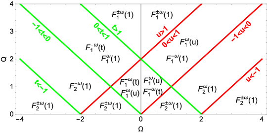
Figure 2: (Color online) Real part $\Delta\Pi^{xx}(\boldsymbol{q},\omega)$ in different regions. Note that we use $t=(Q+\Omega)/2$ and $u=(Q-\Omega)/2$ with dimensionless variables $Q=q/k_{F}$ and $\Omega=\hbar\omega/\epsilon_{F}$ where $k_{F}$ and $\epsilon_{F}$ are Fermi wave vector and Fermi energy respectively. The functions $F^{\pm\omega}_{1}$ and $F^{\pm\omega}_{2}$ are given in the appendix A.

The convenient way to do calculation is to subtract current response of undoped graphene defined as $\Pi^{xx}_{u}({\boldsymbol{q}},\omega)$, from the current response of doped graphene, $\Pi^{xx}_{d}({\boldsymbol{q}},\omega)$ (the subscripts $u,d$ stand for undoped and doped, respectively). We shall then add it back at the end of calculation.

$$\Pi^{xx}_{d}(\boldsymbol{q},\omega)=\Delta\Pi^{xx}(\boldsymbol{q},\omega)+\Pi^{xx}_{u}(\boldsymbol{q},\omega)$$ (13)

$$\Delta\Pi^{xx}(\boldsymbol{q},\omega) =\Pi^{xx}_{d}(\boldsymbol{q},\omega)-\Pi^{xx}_{u}(\boldsymbol{q},\omega)$$ (14)

$$=\frac{g_{s}g_{v}v_{F}^{2}}{4\pi^{2}\hbar}\int_{0}^{k_{f}}kdkd\phi$$

$$\times[P(\boldsymbol{k},\boldsymbol{q},\omega)+P(\boldsymbol{k},\boldsymbol{q},-\omega)].$$

Figure 3: (Color online) Imaginary part $\Delta\Pi^{xx}(\boldsymbol{q},\omega)$ in different regions. Note that we use $t=(Q+\Omega)/2$ and $u=(Q-\Omega)/2$ with dimensionless variables $Q=q/k_{F}$ and $\Omega=\hbar\omega/\epsilon_{F}$ where $k_{F}$ and $\epsilon_{F}$ are Fermi wave vector and Fermi energy respectively. The functions $G^{\pm\omega}_{1}$ and $G^{\pm\omega}_{2}$ are given in the appendix A.

The current response function for the non-interacting undoped graphene can be represented in terms of two functions $F_{0}$ and $G_{0}$ as follows,

$$F_{0} \equiv\real\left[\Pi^{xx}_{0,u}\left(\boldsymbol{q},\omega\right)\right]$$ (15)

$$=-\frac{g_{s}g_{v}}{4\pi\hbar^{2}}\epsilon_{max}-\frac{g_{s}g_{v}}{16\hbar}C_{2}\Theta\left(\left(v_{F}q\right)^{2}-\omega^{2}\right),$$

$$G_{0} \equiv\imaginary\left[\Pi^{xx}_{0,u}\left(\boldsymbol{q},\omega\right)\right]$$ (16)

$$=-\frac{g_{s}g_{v}}{16\hbar}C_{2}\Theta\left(\omega^{2}-\left(v_{F}q\right)^{2}\right),$$

where $C_{2}$ is a function of $(\boldsymbol{q},\omega)$ defined in the appendix A Eq. (42) and subscript zero stands for non-interacting graphene. Here, cutoff energy of Dirac fermions ($\epsilon_{max}$) appears by integrating the imaginary part ($G_{0}$) within a Kramers-Krönig relation. When the cut off tends to infinity, this terms leaves an infinity in the response which can be remedied by normal ordering of the operators employed in calculations of correlators in field theories. A more physical argument to abandon the cutoff dependent term is as follows: In order to have gauge invariant response function and due to the diamagnetic sum rule, cutoff term should be ignored because a real physical system can not respond to the longitudinal vector potential in static limit i.e., static longitudinal current response (LCR) function independent of magnitude of $q$ should be zero. In the same way, in the limit of $q\rightarrow 0$ transverse current response (TCR) function equals to longitudinal ones and it should be zero in static limit [16, 37, 38, 39].

The function $\Delta\Pi^{xx}({\boldsymbol{q}},\omega)$ that adds the effect of doping consists in two complex terms: $P(\boldsymbol{k},\boldsymbol{q},\pm\omega)$ (see Eq. 14). The complete expression and more details of its calculation is given in appendices A and B. We provide the compact form of real (imaginary) part of $\Delta\Pi^{xx}$ in terms of $F_{1}^{\pm\omega}(x)$ or $F_{2}^{\pm\omega}(x)$ ($G_{1}^{\pm\omega}(x)$ or $G_{2}^{\pm\omega}(x)$ ) where $\pm\omega$ refer to the first/second term of Eq. (14), respectively. The regions in the $(q,\omega)$ plane where each function determines the response is shown in Fig. 2 and Fig. 3 where the dimensionless frequency $\Omega=\hbar\omega/\varepsilon_{F}$ and wave vector $Q=q/k_{F}$ are naturally used ($\epsilon_{F}$ and $k_{F}$ are Fermi energy and Fermi wave vector respectively). At the end we need to add the result of undoped response function to obtain the final expression for real and imaginary part of current response function.

Let us emphasize that starting from Eq. (6) and assuming that the polar angle of $\boldsymbol{q}$ with respect to the $x$ axis is $\theta$, the angular dependence of the current response tensor can be separated as,

$$\Pi(\boldsymbol{q},\omega)=B(q,\omega)\mathbb{1}+A(q,\omega)\begin{pmatrix}\cos 2\theta&\sin 2\theta\\ \sin 2\theta&-\cos 2\theta\end{pmatrix}$$ (17)

which is the decomposition of a rank 2 Cartesian tensor in terms of its spherical components with angular independent complex coefficient $A(q,\omega)$ and $B(q,\omega)$.

3 electromagnetic response

Among the interesting features of 2D Dirac materials, their response to electromagnetic fields from the point of view of spin fluctuations deserves investigation. In normal 2D electron gas only a TM mode can propagate [40, 41], while in the Dirac systems already without a ladder resummation correction, the possibility of having a negative imaginary part for the dynamical conductivity provides a new chance for the propagation of TE mode [23]. In this section we would like to explicitly demonstrate the role of non-zero wave vector $\boldsymbol{q}$ in the propagation of electromagnetic modes in graphene. In the absence of a vector $\boldsymbol{q}$, i.e., when $\boldsymbol{q}=0$, the off-diagonal components of the conductivity tensor vanish and the diagonal components are equal and therefore the only remaining component of the reducible rank two conductivity tensor in Eq. (17) is its scalar part given by $B(q=0,\omega)=-i\omega\sigma(\omega)$ where the scalar $\sigma(\omega)$ is the optical conductivity of graphene. Therefore the $\boldsymbol{q}=0$ limit misses the entire tensor structure of the conductivity by reducing it to scalar part.

Starting from Maxwell’s equations, the dispersion relation for the electromagnetic modes in a two dimensional medium for transverse electric and magnetic modes is given by following expressions (for details see Appendix C),

$$1-\frac{2\pi i\omega}{c^{2}\sqrt{q^{2}-\omega^{2}/c^{2}}}\varGamma({\boldsymbol{q}},\omega)=0,~{}~{}~{}~{}~{}\mbox{(TE)}$$ (18)

$$1+\frac{2\pi i\sqrt{q^{2}-\omega^{2}/c^{2}}}{\omega}\varGamma^{\prime}({\boldsymbol{q}},\omega)=0,~{}~{}~{}~{}~{}\mbox{(TM)}$$ (19)

where the functions $\Gamma$ and $\Gamma^{\prime}$ are given by,

$$\varGamma({\boldsymbol{q}},\omega) =\sigma^{yy}({\boldsymbol{q}},\omega)\cos^{2}\theta+\sigma^{xx}({\boldsymbol{q}},\omega)\sin^{2}\theta$$

$$-\sigma^{xy}({\boldsymbol{q}},\omega)\sin 2\theta,$$ (20)

$$\varGamma^{\prime}({\boldsymbol{q}},\omega) =\frac{\sigma^{xx}({\boldsymbol{q}},\omega)\sigma^{yy}({\boldsymbol{q}},\omega)-\sigma^{xy}({\boldsymbol{q}},\omega)\sigma^{xy}({\boldsymbol{q}},\omega)}{\varGamma({\boldsymbol{q}},\omega)},$$ (21)

which reflects how all the components of the two-current correlation tensor determine the propagation of electromagnetic modes in two-dimensional graphene. In the special case of $\boldsymbol{q}=0$, both $\varGamma(\boldsymbol{q}=0,\omega)$ and $\varGamma^{\prime}(\boldsymbol{q}=0,\omega)$ reduce to the scalar conductivity $\sigma(\omega)$ and hence the above dispersion relations for TE and TM modes reduce to those originally used in graphene by Mikhailov and Ziegler [23].

Above relations show angular dependence of $\varGamma$ and $\varGamma^{\prime}$. Let use eliminate conductivity in favor of two-current correlation $\Pi$ by inserting $-i\omega\sigma^{\alpha\beta}(\boldsymbol{q},\omega)=e^{2}\Pi^{\alpha\beta}(\boldsymbol{q},\omega)$ and using the general representation of the conductivity tensor in Eq. (17) to further simplify the dispersion relations of TE and TM modes. This gives a very simple and appealing result:

$$1+\frac{2\pi e^{2}}{c^{2}\sqrt{q^{2}-\omega^{2}/c^{2}}}\Pi^{xx}(q\hat{\boldsymbol{y}},\omega)=0,~{}~{}~{}~{}~{}\mbox{(TE)}$$ (22)

$$1-\frac{2\pi e^{2}\sqrt{q^{2}-\omega^{2}/c^{2}}}{\omega^{2}}\Pi^{xx}(q\hat{\boldsymbol{x}},\omega)=0,~{}~{}~{}~{}~{}\mbox{(TM)}.$$ (23)

The above simplified version emphasizes that we only need one component $\Pi^{xx}$ of the current-current correlation tensor to determine the propagation of EM modes in graphene. The interpretation of the above equations is that TE and TM modes are governed by transverse and longitudinal parts of the two-current response tensor, respectively. Furthermore in the limit of $\boldsymbol{q}=0$ given that $\Pi^{xx}(\omega)=\Pi^{yy}(\omega)=-i\omega\sigma(\omega)/e^{2}$, our equations reduce to those used by Mikhailov and Ziegler [23].

In general an electromagnetic radiation with energies on the scale of eV correspond to wave-lengths which are typically $10^{3}$ times larger that atomic distances. In the reciprocal space this would imply that the wave vector of such EM modes are a tiny fraction $10^{-3}$ of the Brillouin zone. Therefore in terms of the absolute magnitude of the wave vectors of the EM modes it may appear safe to approximate $\varGamma(\boldsymbol{q},\omega)$ and $\varGamma^{\prime}(\boldsymbol{q},\omega)$ with their $\boldsymbol{q}\approx 0$ values which then gives a dispersion relation for the TE and TM modes in terms of the uniform optical conductivity $\sigma(\omega)$ [23]. However the form of Dirac equation means that various correlation are only functions of dimensionless $Q=q/k_{F}$ and $\Omega=\hbar\omega/\varepsilon_{F}$. Therefore as far as the response of 2D Dirac system is concerned, whether we can set $\boldsymbol{q}\approx 0$ or not, depends on the relative magnitude of $q$ and $k_{F}$ and not the absolute magnitude of $q$ which is very small in Brillouin zone scales any way. In the light of recent developments of ultralow doping of graphene, very small values of $k_{F}$ are attainable [12], which then provides access to finite ${\boldsymbol{q}}$ electromagnetic response of graphene. Therefore it is timely to explore aspects of the $q$ (or more precisely $Q$) dependence of the EM response of graphene.

In the ultralow doping regime, not only the $q$-dependence of the EM response is important, but also the many-body interactions become increasingly more important. As a result of stronger many-body interactions in this regime, among other things the many-body effects enhance the Fermi velocity $v_{F}$ of the charge carriers in graphene [12]. In the following sections we will investigate the propagation of TE and TM modes both with and without ladder diagrams due to Hubbard interaction. This will be done for both doped and undoped graphene.

4 Propagation of electromagnetic modes in graphene without ladder corrections

In order to study the propagation of TE mode, first of all we need transverse current response function. However, current response is complex function. Therefore when the imaginary part of it is zero, propagation of TE mode based on Eq. (22) will be governed by real part of the transverse current response. On the contrary when imaginary part is nonzero, the mode will be damped due to dissipation of energy to particle-hole pairs. In this section we will consider graphene without ladder diagram and will focus on the propagation of EM modes in the absence of Stoner excitations. The role of ladder diagrams will be considered in the next section.

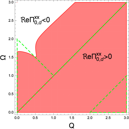
Figure 4: (Color online) The possible region for propagation of TE mode in doped graphene. The white (red) region corresponds to negative (positive) values of$\real\Pi^{xx}_{0,d}(q\hat{\boldsymbol{y}},\omega)$. Dashed green triangles enclose regions where the imaginary part of this function is zero. The vertical edge of the right triangle further extends if we choose to plot a larger region. On the dashed line along the diagonal also the imaginary part is zero. Horizontal and vertical axis are defined as dimensionless wave vector $Q=q/k_{F}$ and energy $\Omega=\hbar\omega/\epsilon_{F}$, respectively.

4.1 TE mode

According to equation (22), the TE mode could propagate when the real part of $\Pi^{xx}(q\hat{\boldsymbol{y}},\omega)$ is a negative quantity. In the case of undoped graphene as can be seen from Eq. (15), the current response is determined by $F_{0}$ which turns out to be a positive quantity. Therefore the TE mode does not exist in undoped graphene. Therefore let us focus on doped graphene.

In the case of doped graphene the doping is characterized with $k_{F}$ corresponding to which an energy scale $\varepsilon_{F}=\hbar v_{F}k_{F}$ exists. Since the response can be organized in terms of dimensionless wave vector $Q=q/k_{F}$ and energy $\Omega=\hbar\omega/\varepsilon_{F}$, we can construct a universal diagram for the propagation of TE mode in doped graphene. In Fig. 4 the white (red) region indicates where $\Pi^{xx}_{0,d}(q\hat{\boldsymbol{y}},\omega)$ is negative (positive). So any possible solution should occur in the white region. In order to avoid damping one must also search in a region where the imaginary part of $\Pi^{xx}_{0,d}(q\hat{\boldsymbol{y}},\omega)$ is zero. Regions where the imaginary part is zero are confined to dashed triangles in this figure. Therefore the undamped TE mode in doped graphene can only exist in the white region inside the left dotted triangle which shares its side with $\Omega$ axis. Indeed at $Q=0$ the possible range of energies corresponding to $1.667<\Omega<2$ which has been found in Ref. [23] is clearly seen in this figure. This figure further shows that the region of $(Q,\Omega)$ space where a possible TE mode can propagate extends up to near $Q\approx 0.5$ and at the same time shrinks by increasing $Q$. Therefore the TE mode found by Mikhailov [23] ceases to exist when the doping is so low that the $k_{F}$ becomes close to $\approx 2$ times the wave-vector of EM radiation.

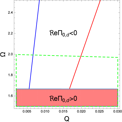
Figure 5: (Color online) Dispersion of TE mode in doped graphene. The white (red) region corresponds to negative (positive) values of $\real\Pi^{xx}_{0,d}(q\hat{\boldsymbol{y}},\omega)$. The dashed green rectangular region is a subset of the triangular region in Fig. 4 and therefore enclose regions where the imaginary part of this function is zero. The solid blue (red) line corresponds to dispersion of TE mode with $v_{F}/c=1/300(1/100)$. Horizontal and vertical axis are defined as $Q=q/k_{F}$ and $\Omega=\hbar\omega/\epsilon_{F}$, respectively.

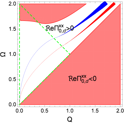
Figure 6: (Color online) Dispersion of TM mode in doped graphene before dressing the polarization function with ladder diagrams. The red (white) area corresponds to the negative (positive) $\real\Pi^{xx}_{0,d}(q\hat{\boldsymbol{x}},\omega)$. Vertical and horizontal axis are $q/k_{F}$ and $\hbar\omega/\epsilon_{F}$, respectively. The area enclosed by dashed green line correspond to the region where $\imaginary\Pi^{xx}_{0,d}(q\hat{\boldsymbol{x}},\omega)$ is zero. The blue (red) line is the dispersion of TM mode with $v_{F}/c=1/300$ ($1/100$). Outside the green triangular region, TM mode will be damped by the non zero $\imaginary\Pi^{xx}_{0,d}(q\hat{\boldsymbol{x}},\omega)$. This damped behavior is represented by broadening which arises from the imaginary part of $Q$. Note that for visibility purpose we have magnified the broadening by a factor of $10$.

So far we have not really solved Eq. (22) and have discussed on general grounds the circumstances under which a possible solution to this equation may exist. To solve the equation and obtain the dispersion relation, one needs the numerical value of the $v_{F}/c$. The blue (red) solid dispersion relation in Fig. 5 denote the TE mode for two different values of the parameter $v_{F}/c=1/300$ ($1/100$). The solution to Eq. (22) in the white region inside the left triangle exists only up to a certain value of $Q_{max}$, the value of which is controlled by the numerical value of the parameter $v_{F}/c$. For example when $v_{F}/c=1/300$, we find $Q_{max}\approx 0.0066$ while if $v_{F}/c=1/100$ (due to enhancement of the Fermi velocity in ultralow doped graphene) we have $Q_{max}\approx 0.02$. Beyond this points there are no real $(Q,\Omega)$ solutions to the TE mode in graphene.

4.2 TM mode

The propagation of TM mode is governed by Eq. (23) which includes the longitudinal current correlation $\Pi^{xx}(q\hat{\boldsymbol{x}},\omega)$. The solutions to TM mode dispersion can exist only when real part of this quantity is positive. In the case of undoped graphene again we need Eq. (15) from which the longitudinal (i.e., $\theta=0$) part of the response turns out to be negative and hence forbids the propagation of TM mode in undoped graphene.

In Fig. 6 we have plotted the sign structure of the $\Pi^{xx}_{0,d}(q\hat{\boldsymbol{x}},\omega)$. For the positive (negative) real part where the TM mode can (can not) have a solution we have used the white (red) color. Again the region where the imaginary part of this function is zero is enclosed by dashed green line. Therefore the intersection of white region and dashed triangle is a region where undamped TM mode can exist, while the white region outside the dashed green triangle is the region where the TM mode is damped by dissipating energy to particle-hole pairs. In the optical limits i.e., $q=0$ this white window is $\omega\lesssim 1.667$ and by increasing momentum $q$ it will be slightly more restricted as in Fig. 6. The blue and red solid lines are the solutions of Eq. (23) for representative value of $v_{F}/c=1/300$ and $v_{F}/c=1/100$. The group velocity of TM mode is larger when $v_{F}/c$ is larger at very small momenta. When these dispersion relation cross the boundary of the dashed triangle the imaginary part of longitudinal current response will be nonzero which causes the TM mode to dissipate energy to particle-hole pairs and acquire damping. The broadening of the dispersion indicated in Fig. 6 is a measure of the imaginary part $Q^{\operatorname*{\prime\prime}}$ of the wave vector $Q$. In appendix D we show how the imaginary part $Q^{\operatorname*{\prime\prime}}$ is related to the imaginary part of $\Pi_{0,d}^{xx}$. See Eq. (96). Note that in this figure to clearly represent the damping we have multiplied the broadening by a factor of $10$.

5 Dressing the polarization by ladder diagrams

So far we have shown that equations (22) and (23) give the dispersion of TE and TM modes in terms of transverse and longitudinal parts of the two-current tensor. In this section we would like to study which one of the above responses receives corrections from the ladder diagrams generated by the Hubbard interaction. For this purpose we start by the continuity equation which is given by,

$$\divergence\boldsymbol{\hat{j}}(\boldsymbol{r},t)=\partial_{t}\hat{\rho}(\boldsymbol{r},t),$$ (24)

and relates current and density operator. As a consequence of this, current and density correlation function [16, 17] are related by,

$$\chi(q,\omega)=\frac{q}{\omega^{2}}[\hat{\boldsymbol{j}}_{x},\hat{\rho}_{-q}](q\boldsymbol{\hat{x}},\omega)+\frac{q^{2}}{\omega^{2}}\Pi^{x,x}(q\boldsymbol{\hat{x}},\omega).$$ (25)

In the right hand side of this equation first term turns out to be a real quantity which is proportional to cutoff parameter and will be canceled by similar cutoff term in the second term. Therefore the longitudinal current response function has a direct relation with density correlation function,

$$\chi(q,\omega)=\frac{q^{2}}{\omega^{2}}\Pi^{xx}(q\boldsymbol{\hat{x}},\omega).$$ (26)

Therefore, if any correction such as inclusion of ladder diagrams causes some changes in the behavior of (electric charge) density response, it will directly affect the longitudinal current response via Eq. (26). Normally used approximation which corresponds to random phase approximation is to use $\chi=\chi_{0}$ which corresponds to the first term in Fig. 1b. However, as will be shown shortly, the inclusion of ladder diagrams will totally change the structure of $\chi$, and hence will drastically affect the propagation of TM mode in graphene. This will in turn modify only the propagation of TM mode. Therefore in principle the TM mode receives corrections from the inclusion of dressing of the ladders by Stoner PH processes, while the TE mode is not affected by such diagrams as they ultimately arise from a density-density (Hubbard) interaction. Only Thirring type (current-current) interactions are able to modify the TE mode which maybe relevant for Thirring matter, but not to graphene as an example of Dirac systems on which we are focused in this paper.

Let us point out that the particle-hole pairs propagating along the rungs of ladder have two options when they enter a dashed interaction line that represents the Hubbard interaction: They can either flip their spins for which the interaction will chagne sign to $-U$; or they can keep going with no spin flip [2, 42, 43, 44, 35] for whith the Hubbard term keeps its original sign $+U$. If one tries to construct a (particle-number) conserving approximation in the sense of Baym and Kadanoff [45], both sets of diagrams are relevant and none of them can be neglected in the interest of the other. This is the essence of fluctuation-exchange approximation (FLEX) which in a sense Fierz decomposes the (short range) Coulomb interaction into various channels such as singlet or triplet PH channels, and similar particle-particle channels. For any model Hamiltonian, the properties of the system decide fluctuations in which channel are to be enhanced or suppressed. The nature of particle-hole continuum in graphene is such that provides a unique opportunity of which the spin-flip fluctuations can take advantage and develop a coherent pole which indicates that they bind into triplet bound states of particle-hole pairs below the continuum of free particle-hole excitations [29, 30, 31, 34]. The very same ladder summation mechanism when accounted for in the EM response of the system, generates a singularity in the polarization function that arises from proliferation of Stoner PH excitations along the ladder rung. Therefore the major role is played by the spin-flip processes that run across the rungs of the ladder.

Putting the above words on a formal language has been already done in the literature and is known as the fluctuation exchange (FLEX) approximation which is a natural language to address the role of separate channels for fluctuations of various quantities [4, 2].

For short range interactions where Hubbard $U$ is independent of momentum, the ladder series in Fig. 1b can be easily summed. This has been already done in the FLEX approximation in a more complete form that takes both spin-flip and non-spin-flip processes along the ladder rung. Since PH fluctuations in both spin-flip and non-spin-flip channel will ultimately lead to fluctuations of the electric charge, the effective interaction determining the dielectric properties will have contributions from both channels. The part of effective interaction that is attached to two bare interaction lines and defines the effective charge polarization, in the FLEX approximation is given by [2, 42, 43, 46, 47],

$$\chi^{\rm eff}_{\rm FLEX}(q,\omega)= \frac{3}{2}\bigg{[}\frac{\chi_{0}(q,\omega)}{1+U\chi_{0}(q,\omega)}-\chi_{0}(q,\omega)\bigg{]}+$$

$$\frac{1}{2}\bigg{[}\frac{\chi_{0}(q,\omega)}{1-U\chi_{0}(q,\omega)}-\chi_{0}(q,\omega)\bigg{]}+$$

$$\chi_{0}(q,\omega)$$ (27)

where $\chi_{0}({\boldsymbol{q}},\omega)$ is density response function of non-interacting system without the spin degeneracy. Note that despite its RPA-looking form, the above formula is related to ladder summation. It is only due to momentum independence of Hubbard $U$ interaction that the ladder summation acquires such a simple form. The first and second lines represent the contribution of spin-flip and non-spin-flip channels, respectively. Note that as expected from our simple argument in the introduction, the sign of interaction in the spin-flip channel differes from the non-spin-flip channel. As a quick check, the terms in the brackets vanish when we set $U=0$ and one is left with empty bubble $\chi_{0}$ only. As we will see shortly, the sign change $U\to-U$ in the denominator of the spin-flip channel, will make the $\chi^{\rm eff}_{\rm FLEX}$ positive and therefore Eq. (23) can have a solution in undoped graphene.

As pointed out earlier, the longitudinal (density) interactions of the Coulomb type are not going to affect the propagation of TE mode. So we focus on the TM mode and consider the role of triplet fluctuations on propagation of the TM mode in graphene. Let us start by the undoped graphene first.

5.1 Undoped graphene

As we pointed out earlier, propagation of TM mode in undoped graphene is not possible as a result of negative current response function. When the contributions from spin flip channel of the ladder diagrams that corresponds to the first line of Eq. (27) is taken into account, the negative sign of $\chi_{0}$ below the PH continuum can generate a pole in the ladder summation of spin-flip processes. This gives rise to a positive $\chi^{\rm eff}_{\rm FLEX}$ which in turn can give rise to propagating solutions in Eq. (23). The ladder summation with long-ranged (momentum dependent) interactions can be performed under very stringent conditions which is valid for $\omega\approx qv_{F}$ [35]. In this case, a singularity in the density response can be produced by the ladder diagrams and gives rise to a damped solution in Eq.(23). We find that this solution is $\omega\approx 1.15qv_{F}$ which lies above the $\omega=qv_{F}$ line where the density of free PH pairs is non-zero and therefore becomes damped. Inclusion of ladder diagrams reduces the imaginary part of $\chi$ and thereby reduces the damping, but this is not sufficient. A better situation can be generated with short range interactions (which is already strong enough in graphene) that enhances spin fluctuations This enhancement is precisely encoded in the denominator of the first line of Eq. (27) and is known as Stoner enhancement [1].

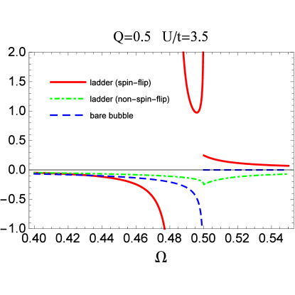
Figure 7: (Color line) Separate contribution of bare bubble (blue dashed line) corresponidng to no ladder correction, spin-flip ladder diagrams (red solid line) and non-spin-flip ladders (green dotted dashed line). These terms when added up give the effective charge polarization in Eq. (27) for $U/t=3.5$ and $Q=0.5$ in undoped graphene. Note that in undoped graphene we use the following definition $Q=\hbar qv_{F}/t$ horizontal axis is $\Omega=\hbar\omega/t$. As can be seen only the red line allows $\chi^{\rm eff}$ to become positive and hence the TM mode equation can develope possible solutions.

To see the structure of sings, in Fig. 7, we have plotted the charge polarization arising from various terms of Eq. (27). The bare polarization (blue dashed line) corresponds to the first term in the right hand side of Fig. 1b and is given in third line of Eq. (27). The first line of this equation corresponds to the rest of diagrams in Fig. 1b and is denoted by red solid line in Fig. 7. Finally the second line of Eq. (27) corresponds to ladder diagrams along the rung of which spins do not flip are denoted by green dashed line. This figure is produced for $U/t=3.5$ and $Q=0.5$ and demonstrates how the inclusion of the ladder diagrams and the spin-flip fluctuations encoded in these diagrams can make the resulting $\chi^{\rm eff}$ positive and hence lead to a solution for the TM mode Eq. (23). This figure clearly shows that the dominant effect of ladder diagram resummation comes from spin-flip excitations and therefore the resulting divergence is the Stoner enhancement.

Now that we are convinced about the special role of Stoner enhancement in making the $\chi^{\rm eff}$ positive, and hence providing a chance for a solution to the TM mode Eq. (23), let us study the dependence of solutions to the Hubbard parameter $u=U/t$ which controls the strength of spin-fluctuations. To this end, in Eq. (23) we place the $\Pi^{xx}$ in one side and the rest in the other side of equation and in $\Pi^{xx}$ we take full account of all channels in Eq. (27).

In the left panel of Fig. 8 we have plotted the the $\Pi^{xx}$ for various values of $u=U/t$ and assumed that the surrounding medium is such that the effective dielectric constant is $\epsilon\sim 20$. In the right panel of this figure we have extracted the dispersion of TM mode for $U/t=3.5$ and $\epsilon=20.6$. As can be seen from panel (a) there are always two solutions, one is immediately below the PH continuum, and the other is well below the PH continuum and therefore protected from damping. Note how larger Hubbard parameter increases the separation of TM mode solution from the PH continuum and hence leads to better protection from damping. In panel (b) of this figure, for a fixed $u=U/t=3.5$ adopted from Ref. [27] for graphene, and for surrounding medium dielectric constant of $\epsilon=20.6$ we plot the dispersion of TM modes in black. Both TM dispersions start at a threshold wave vector. Increasing the effective dielectric constant of the surrounding medium brings this threshold wave vector to smaller values.

a)

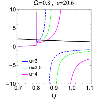
b)

(

(a)

(

(b)

Figure 8: (Color line) (a) Solutions for TM modes in undoped graphene within the ladder resummation approximation for different value of repulsive Hubbard parameter $u=U/t$. Here grpahene layer is surrounded by dielectric constant $\epsilon\sim 20.6$. In panel (a) the thin lines (blue dashed, green dotted dashed, pink solid) are plot of $\Pi^{xx}$ within the ladder approximation, Eq. (27) and the black (thick solid) line is plot of other side of equation obtained from re-arranging Eq. (23). Panel (b) depicts the dispersion of TM modes for indicated values of $U$ and $\epsilon$. The axes are defined by $Q=\hbar qv_{F}/t$ and $\Omega=\hbar\omega/t$.

5.2 Extrinsic graphene

So far we have seen that the modifications of the charge polarization by spin-flip PH fluctuations can in principle give rise to a TM mode solution in undoped graphene which can never happen if no spin-flip fluctuations are taken into account. Now let us turn our attention to dopped graphene. In doped graphene, the TM modes are sustained in the form of plasmon excitations of the chiral electron gas [18]. Now the question is whether the inclusion of the spin-flip ladder diagrams will affect TM mode or not? We will shortly see that the generic role of itinerant spin fluctuations in graphene is to lower the energies of TM modes.

To elucidate the peculiar role of spin fluctuations on the TM mode of doped graphene, in Fig. 9 we plot the dispersion of the TM mode in doped graphene for three different situations: bare (blue dashed line) corresponding to no ladder corrections, and full ladder approximation of Eq. (27). The black (dotted dashed) line corresponds to the effective dielectric constant $\epsilon=1$ and the red (solid) line corresponds to $\epsilon=5$ as indicated in the legend in both panels. The value of Hubbard $U$ in both panels is $U/t=3.5$. In panel (a) is for typically doped graphene with $t/\mu=3.5$ , $v_{F}/c=1/300$ while the panel (b) is for ultra-low doped graphene $t/\mu=35$, $v_{F}/c=1/100$. As can be seen in all cases the role of triplet PH fluctuations encoded in the ladder summation is to lower the energy of TM mode. If graphene is surrounded with an dielectric constant $5$, the dispersion of the TM mode will come closer to the $\Omega=Q$ line. The ultra-low doped graphene shows the same features but with differences which arises of smaller Fermi surface and bigger Fermi velocity. The dispersive mode inside (outside) of the area with green dashed line is undamped (damped). The common feature of all dispersions is that once the ladder resummation is included, the energy of the TM mode will be lowered.

a)

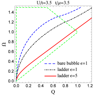
b)

(

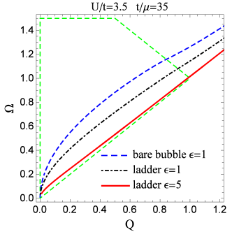
(a)

(

(b)

Figure 9: (Color line) Propagation of TM mode in doped grpahene. We compare the bare (blue dashed), with full FLEX charge polarizations as indicated in the legend for medium dielectric constants of $1$ (black, dotted dashed line) and $5$ (red, solid line). Panel (a) and (b) show dispersion of TM mode in typically doped ($v_{F}/c=1/300$ , $t/\mu=3.5$) and ultra-low dopped ($v_{F}/c=1/100$ , $t/\mu=35$) graphene. Here horizontal and vertical axes are $Q=\hbar qv_{F}/t$ and $\Omega=\hbar\omega/t$ respectively where $\mu$ is Fermi energy, $t$ hopping amplitude.

An interesting observation in Fig. 9 is that when the Fermi velocity is parametrically larger (which can be achieved in ultra-low doping by renormalization [12]), inclusion of the spin-flip particle-hole fluctuations gives rise to a branch of TM mode which almost disperses at the Fermi velocity. The conclusion is that the total spin of the particle-hole pairs has a significant effect on the propagation of the TM mode, and the TM mode can take advantage of the minus sign in the triplet channel of Eq. (27) to lower its energy. This can be interpreted as follows: An incoming photon propagator creates an electron-hole pair. This Electron-hole pair due to strong spin fluctuations which can be thought of as an effective boson that mediates spin-flip across the ladder, gives rise to a form of dressing which makes $\chi{\rm eff}$ positive and hence can furnish a solution to Eq. (23). At the end of this process, the end particle-hole pairs recombine to emit a photon.

6 Summary and conclusion

In this work we have investigated the role of Stoner enhancement which is generated by strong enough short-range interactions – and is formalized as series of ladder diagrams as in Fig. 1 – on the propagation of electromagnetic modes. An incident light generates a PH pair. This pair is then resonantly scattered as shown in the ladder summation in Fig. 1.

We have chosen to demonstrate this effect in graphene, because: (i) Graphene has large enough Hubbard $U\sim 10$ eV. (ii) When doped it supports an interesting TE mode. (iii) The nature of PH continuum is such that the spin-flip fluctuations can be resummed into a coherent pole that lies outside the PH continuum. Under such a suitable circumstances, the inclusion of ladder diagrams has its most drastic effect in the spin-flip channel as in this channel the sign of $U$ is reversed: $U\to-U$. This sign reversal gives rise to a resonance in undoped graphene where it gives rise to a branch of TM mode very well separated from the PH continuum. This minus sign picked from fermionic anti-commutations on going from non-spin-flip to spin-flip channel provides a unique chance to get a solution to Eq. (23) which is otherwise (i.e. without ladder corrections) impossible. Realization of this effect requires high dielectric surrounding medium.

In doped graphene an intrinsic momentum scale $k_{F}$ and energy scale $\epsilon_{F}$ emerge and hence physical properties are functions of the ratio ${\boldsymbol{q}}/k_{F}$ and $\hbar\omega/\epsilon_{F}$. Possibility of ultralow doping in graphene, provides access to finite ${\boldsymbol{q}}$ behavior of the optical response. Inclusion of ladder corrections slightly modifies the TM modes of doped graphene by generically lowering their energies. In the ultralow doped case where the Fermi velocity is parametrically large, this effects becomes substantial. This lowering of energy of the TM mode can be traced back to the minus sign picked up in the spin-flip channel. The ladder corrections do not affect the TE modes [23] of the doped graphene.

What do the spin-flip particle-hole fluctuations do in conducting states other than graphene, e.g. in a normal metal? The essential property of graphene is reflected in the existence of a region below the continuum of PH excitations. The particle-hole continuum of normal conductors (i.e. Fermi liquids) does not allow for such windows below the continuum. Such a window below the continuum when combined with relatively large on-site Coulomb repulsion $U/t\sim 3.5$ [27] can enhance the spin fluctuations. But since the spins are not localized, spin-1 fluctuations also contribute to the charge polarization, albeit with effectively reversed sign of Hubbard $U$. In normal conductors when the triplet fluctuations want to bring down the energy of the TM mode, the mode sinks more into the continuum of free particle-holes and gets quickly damping. Moreover, in most normal conductors the screening is very effective, and conduction bands are very wide, such that the ratio of the Hubbard $U$ and hopping is not large. Therefore the chiral nature of fermions in graphene along with the triplet fluctuations arising from Hubbard interactions join hands to give a unique chance for the propagation of TM mode in undoped graphene.

The nature of PH continuum in higly oriented pyrolytic graphite – above the energy scale of $\sim 50$ meV related to inter-layer hopping between the constituting graphene layers – is quite similar to graphene [29]. Therefore the same effects are expected for graphite as well. Propagation of circularly polarized EM radtion with graphene/graphite may also receive corrections from spin fluctuations. This might have relevance to natural birefringence observed in a closely related material, graphite [48, 49].

Appendix A Current response function

Electromagnetic response of graphene is characterized by the tensor form of current correlation function Eq. (6) in the terms of form factor elements. If we substitute $\phi_{k}$ by $\phi_{k}+\theta$ in current correlation function Eq. (6), we obtain,

$$\cos(\phi_{k}+\phi_{k+q})=\frac{k\cos 2(\phi_{k}+\theta)+q\cos(\phi_{k}+2\theta)}{|\boldsymbol{k}+\boldsymbol{q}|},$$ (28)

$$\sin(\phi_{k}+\phi_{k+q})=\frac{k\sin 2(\phi_{k}+\theta)+q\sin(\phi_{k}+2\theta)}{|\boldsymbol{k}+\boldsymbol{q}|},$$ (29)

where

$$|\boldsymbol{k}+\boldsymbol{q}|=\sqrt{k^{2}+q^{2}+2kq\cos\phi}~{}.$$ (30)

The advantage of point of this change of variable is that allows us to represent each element of tensor current correlation function in terms of one function, e.g., $\Pi^{x,x}(\boldsymbol{q},\omega)$. By using properties of this transformation the new representation of tensor current correlation function in terms of $\Pi^{x,x}(\boldsymbol{q},\omega)$ will be given by Eq. (9). In what follow, we use this representation of tensor current correlation function.

We better define the difference between the corresponding response between doped and undoped case for $xx$ component of current response tensor as,

$$\Delta\Pi^{x,x}(\boldsymbol{q},i\omega_{n}) =\Pi^{x,x}_{d}(\boldsymbol{q},i\omega_{n})-\Pi^{x,x}_{u}(\boldsymbol{q},i\omega_{n})$$ (31)

$$=\frac{g_{s}g_{v}v_{F}^{2}}{4\pi^{2}\hbar}\int_{0}^{k_{f}}kdkd\phi$$

$$\times[P(\boldsymbol{k},\boldsymbol{q},i\omega_{n})+P^{*}(\boldsymbol{k},\boldsymbol{q},i\omega_{n})],$$

where the subscripts $u,d$ stand for undoped and doped, respectively, and

$$P({\boldsymbol{k}},{\boldsymbol{q}},i\omega_{n})= \frac{(i\omega_{n}+v_{F}k)}{(i\omega_{n}+v_{F}k)^{2}-v_{F}^{2}|{\boldsymbol{k}}+{\boldsymbol{q}}|^{2}}$$ (32)

$$+\frac{v_{F}k\cos 2(\phi+\theta)}{(i\omega_{n}+v_{F}k)^{2}-v_{F}^{2}|{\boldsymbol{k}}+{\boldsymbol{q}}|^{2}}$$

$$+\frac{v_{F}q\cos(\phi+2\theta)}{(i\omega_{n}+v_{F}k)^{2}-v_{F}^{2}|{\boldsymbol{k}}+{\boldsymbol{q}}|^{2}},$$

which has a nice quadratic expressions in the denominator. Here, $i\omega_{n}$ is $\omega+i\eta$ which points to the complex frequency domain with infinitesimal imaginary part $\eta$. One can easily see the terms which include $\sin 2\phi$ or $\sin\phi$ don’t have any contribution hence, in the following calculation we eliminate them in the representation of $P({\boldsymbol{k}},{\boldsymbol{q}},i\omega_{n})$ and it’s conjugate and proceed our calculation by using complex integration.

A.1 real part

As a result of substituting $i\omega_{n}$ by $\omega$, the real part of response function is defined by

$$\Delta\Pi^{xx}(\boldsymbol{q},\omega) =\frac{g_{s}g_{v}v_{F}^{2}}{4\pi^{2}\hbar}\int_{0}^{k_{F}}kdkd\phi$$ (33)

$$\times[P({\boldsymbol{k}},{\boldsymbol{q}},\omega)+P({\boldsymbol{k}},{\boldsymbol{q}},-\omega)].$$

Here, $P({\boldsymbol{k}},{\boldsymbol{q}},-\omega)$ is a real function. For this purpose we define $z=e^{i\phi}$ and $\Delta=(v_{f}^{2}q^{2}-\omega^{2}-2\omega v_{f}k)/(2v_{f}^{2}kq)$ in order to do angular integration,

$$\int d\phi P(\boldsymbol{k},\boldsymbol{q},\omega)=\frac{-i}{2v_{F}^{2}kq}\oint\frac{dz}{z^{2}}\frac{B_{z}(\boldsymbol{k},q,\omega)}{z^{2}+2\Delta z+1}$$ (34)

where,

$$B_{z}(\boldsymbol{k},q,\omega)= (\omega+2v_{F}k\sin^{2}\theta)z^{2}+2v_{F}k\cos 2\theta(z^{2}+1)^{2}+$$ (35)

$$v_{F}q\cos 2\theta z(z^{2}+1).$$

The roots of denominator are: a second order root at $z_{0}=0$ and two first order roots at $z_{\pm}=-\Delta\pm\sqrt{\Delta^{2}-1}$ when $\Delta\geq 1$ and $z^{\prime}_{\pm}=-\Delta\pm i\sqrt{1-\Delta^{2}}$ when $\Delta<1$. Among these roots, whichever placed within the unit circle contribute to the integration. We can summarize result of integration by,

$$\int d\phi P(\boldsymbol{k},\boldsymbol{q},\omega)=Res(z_{0})+\text{sgn}(\Delta)Res(z_{+})\Theta(|\Delta|-1)$$ (36)

with

$$Res(z_{0}) =\frac{2\pi\cos 2\theta}{v_{F}q}\omega(\omega+2v_{F}k),$$ (37)

and

$$Res(z_{+})= \frac{2\pi}{\sqrt{\Delta^{2}-1}}\bigg{[}2(\omega+v_{F}k)\cos^{2}\theta-$$ (38)

$$\cos 2\theta\frac{(\omega+2v_{F}k)^{2}((v_{F}q)^{2}-\omega^{2})}{2v_{F}^{3}kq^{2}}\bigg{]}.$$

Here, we refuse to include residue in $z^{\prime}_{\pm}$ in Eq. 36, because when $|\Delta|<1$ both of roots simultaneity lie in the unit circle and due to $Res(z^{\prime}_{-})=-Res(z^{\prime}_{+})$ their contribution in Eq. 36 will be cancel each other. Meanwhile the residue in $z_{-}$ is equal to $-Res(z_{+})$. The symmetry of real response function to frequency can easily seen in Eq. 33. Therefor it is just sufficient to proceed our calculation for positive $\omega$ and then pick the even part of $\omega$ dependence at the end. The final process is integration over momentum $k$. The first part of integration ($Res(z_{0})$) is proportional to $\omega^{2}+v_{F}k\omega$ from which the second term will be dropped upon $\omega\rightarrow-\omega$ in $P(\boldsymbol{k},\boldsymbol{q},-\omega)$. Finally the contribution of this root is $-\frac{g_{s}g_{v}}{2\pi}\epsilon_{F}(\omega/\hbar v_{F}q)^{2}\cos 2\theta$. The result of integration of $Res(z_{+})$ depends on the relation between $\omega$ and $v_{F}q$ as follows,

$$-\frac{g_{s}g_{v}}{2\pi}\frac{\epsilon_{F}\omega^{2}}{(\hbar v_{F}q)^{2}}\cos 2\theta+\frac{g_{s}g_{v}s(\Delta)}{16\pi\hbar}\Theta(v_{F}q-|\omega|)$$

$$\times\left[C_{1}G\left(x\right)+C_{2}\sin^{-1}\left(x\right)\right]^{X}_{0}\equiv\left[F_{1}^{\pm\omega}(x)\right]^{X}_{0}$$ (39)

$$-\frac{g_{s}g_{v}}{2\pi}\frac{\epsilon_{F}\omega^{2}}{(\hbar v_{F}q)^{2}}\cos 2\theta+\frac{g_{s}g_{v}\text{s}(\Delta)}{16\pi\hbar}\Theta(|\omega|-v_{F}q)$$

$$\times\left[-C_{1}G\left(x\right)+C_{2}\cosh\left(x\right)\right]^{X}_{0}\equiv\left[F_{2}^{\pm\omega}(x)\right]^{X}_{0}$$ (40)

where

$$C_{1}=\frac{\omega^{2}\cos^{2}\theta-\left(\omega^{2}-\left(v_{F}q\right)^{2}\right)\sin^{2}\theta}{\sqrt{\left|\omega^{2}-\left(v_{F}q\right)^{2}\right|}},$$ (41)

$$C_{2}=\frac{\omega^{2}\cos^{2}\theta+\left(\omega^{2}-\left(v_{F}q\right)^{2}\right)\sin^{2}\theta}{\sqrt{\left|\omega^{2}-\left(v_{F}q\right)^{2}\right|}},$$ (42)

$$G\left(x\right)=\left(\frac{2xv_{F}k_{F}+\omega}{v_{F}q}\right)\sqrt{\left|\left(\frac{2xv_{F}k_{F}+\omega}{v_{F}q}\right)^{2}-1\right|},$$ (43)

$$\cosh\left(x\right)=ln\left[\left|\frac{2xv_{F}k_{F}+\omega}{v_{F}q}\right|+\sqrt{\left|\left(\frac{2xv_{F}k_{F}+\omega}{v_{F}q}\right)^{2}-1\right|}\right],$$ (44)

$$\sin^{-1}\left(x\right)=\sin^{-1}\left(\frac{2xv_{F}k_{F}+\omega}{v_{F}q}\right).$$ (45)

Here $\pm\omega$ in both functions refer to the integration over $P(\boldsymbol{k},\boldsymbol{q},\pm\omega)$ and the function $s(\Delta)$ is basically $sgn(\Delta)\Theta\left(|\Delta|-1\right)$, and upper limit $X$ are functions of $q,\omega,k_{F}$. Before finding the integration range, note that the functional form of the above expression at $x=0$ is purely odd with respect to $\omega$ and therefore drops out by adding the $\omega\to-\omega$. We therefore need to carefully determine the upper limit $X$ which was shown in Fig. (2).

A.2 Imaginary part

In Eq. 31, if we consider imaginary contribution of $P^{*}(\boldsymbol{k},\boldsymbol{q},i\omega_{n})$ and $P(\boldsymbol{k},\boldsymbol{q},i\omega_{n})$, imaginary part of $\Delta\Pi$ will be derived. Again we focus on first term of this representation i.e., $P(\boldsymbol{k},\boldsymbol{q},\pm\omega)$ and repeat similar calculation for other term. As a first step we profit by presence of infinitesimal imaginary part in $\eta$ in $\omega+i\eta$ which causes a delta function of the form

$$\imaginary[P(\boldsymbol{k},\boldsymbol{q},\omega)]\equiv\frac{M(\boldsymbol{k},{\boldsymbol{q}},\omega)}{4(\omega+v_{F}k)^{2}}\delta(\xi),$$ (46)

where,

$$M(\boldsymbol{k},{\boldsymbol{q}},\omega)= \omega^{2}+2\omega v_{F}k-v_{F}^{2}q^{2}-2v_{F}^{2}kq\cos\phi$$ (47)

$$-2(\omega+2v_{F}k\sin^{2}\theta+2v_{F}k\cos 2\theta\cos^{2}\phi$$

$$+v_{F}q\cos 2\theta\cos\phi)(\omega+v_{F}k),$$

and

$$\xi= \frac{\omega^{2}+2\omega v_{F}k-v_{F}^{2}q^{2}-2v_{F}^{2}kq\cos\phi}{2(\omega+v_{F}k)}.$$ (48)

In oder to do angular integration we consider $\xi$ as a function of $\phi$ and use $\delta[\xi(\phi)]=\frac{\delta(\phi-\phi_{0})}{|\partial_{\phi}\xi(\phi)|_{\phi_{0}}|}$ where $\cos\phi_{0}=-\vartheta$ then do integration on momentum $k$:

$$\int d\phi\imaginary[P({\boldsymbol{k}},{\boldsymbol{q}},\omega)]=\pi\frac{\gamma_{\vartheta}(k,{\boldsymbol{q}},\omega)}{v_{F}^{2}kq\sqrt{1-\vartheta^{2}}},$$ (49)

with

$$\gamma_{\vartheta}(k,{\boldsymbol{q}},\omega)=\omega+2v_{F}k\sin^{2}\theta+2v_{F}k\vartheta^{2}\cos 2\theta-v_{F}q\vartheta\cos 2\theta.$$ (50)

Here, the significant is limitation on the value of $\cos$ which causes $-1\leq\vartheta\leq 1$. Applying this constriction to integration on momentum $k$ leads to the answer zero in the area with $\omega>v_{f}q$. By applying the same process to second term of $\Delta\Pi$ we get,

$$\int d\phi\imaginary[P({\boldsymbol{k}},{\boldsymbol{q}},-\omega)]=-\pi\frac{\gamma_{\vartheta^{\prime}}(k,{\boldsymbol{q}},-\omega)sgn(\omega-v_{F}k)}{v_{F}^{2}kq\sqrt{1-\vartheta^{\prime 2}}},$$ (51)

where

$$\vartheta^{\prime}=\frac{v_{F}^{2}q^{2}-\omega^{2}+2\omega v_{F}k}{2v_{F}^{2}kq},$$ (52)

and $\gamma_{\vartheta^{\prime}}$ is otbained from $\gamma_{\vartheta}$ by substituting $\vartheta^{\prime}$ for $\vartheta$. Then the integration on $k$ space gives the following results:

$$\mp\frac{g_{s}g_{v}}{16\pi\hbar}\Theta(|\omega|-v_{F}q)\left[C_{1}G\left(x\right)+C_{2}\sin^{-1}\left(x\right)\right]^{X}_{X^{\prime}}$$

$$\equiv\left[G_{1}^{\pm\omega}(x)\right]^{X}_{X^{\prime}},$$ (53)

and

$$\pm\frac{g_{s}g_{v}}{16\pi\hbar}\Theta(v_{F}q-|\omega|)\left[-C_{1}G\left(x\right)+C_{2}\cosh\left(x\right)\right]^{X}_{0}$$

$$\equiv\left[G_{2}^{\pm\omega}(x)\right]^{X}_{0},$$ (54)

where the definition of $C_{1},C_{2}$ and $G,\cosh,\sin^{-1}$ are already given in Eqns. (41) to (45). The integration limits $X$ and $X^{\prime}$ will be determine by the value of $v_{F}q$, $v_{F}k_{F}$ and $\omega$. Here the superscript $\pm\omega$ indicates whether the first and second term in Eq.31 is being dealt with.

Appendix B Response of quantum matter to the transverse magnetic filed

In this appendix we present details of the electromagnetic response of single layer of graphene to electromagnetic fields with emphasize on the tensor nature of the conductivity tensor. The following derivation holds for any quantum material which is specified by a two dimensional conductivity tensor $\sigma({\boldsymbol{q}},\omega)$. We assume that graphene is placed in $xy$ plane, and therefor the electric field in $z$ direction should be decaying away from the graphene plane [40] i.e., $\boldsymbol{E}({\boldsymbol{q}},\omega)=\boldsymbol{E}e^{(i{\boldsymbol{q}}.\boldsymbol{r}-\zeta|z|-i\omega t)}$ with $\zeta=\sqrt{q^{2}-\omega^{2}/c^{2}}$. In what follow, we proceed from Maxwell equations in Gaussian units for the rest of calculation. Let us start with,

$$\nabla(\nabla.\vec{\boldsymbol{E}})-\nabla^{2}\boldsymbol{E}=\frac{1}{c^{2}}\big{(}4\pi i\omega\boldsymbol{\sigma}({\boldsymbol{q}},\omega)+\omega^{2}\big{)}\boldsymbol{E}.$$ (55)

In the case of graphene conductivity is a tensor rather than a scalar which is represent by Eq. 57. Symmetry of Hamiltonian implies that $\sigma^{xy}({\boldsymbol{q}},\omega)=\sigma^{yx}({\boldsymbol{q}},\omega)$ and is defined by[50]

$$\boldsymbol{J}({\boldsymbol{q}},\omega)=\boldsymbol{\sigma}({\boldsymbol{q}},\omega)\boldsymbol{E},$$ (56)

with

$$\boldsymbol{\sigma}({\boldsymbol{q}},\omega)=\begin{pmatrix}\sigma^{xx}({\boldsymbol{q}},\omega)&\sigma^{xy}({\boldsymbol{q}},\omega)\\ \sigma^{yx}({\boldsymbol{q}},\omega)&\sigma^{yy}({\boldsymbol{q}},\omega)\end{pmatrix}$$ (57)

Let us look at the Cartesian components of Eq. 55. Along $x$ we have,

$$-q_{x}q_{y}E_{y}+q_{y}^{2}E_{x}+iq_{x}\frac{\partial E_{z}}{\partial z}-\frac{\partial^{2}E_{x}}{\partial z^{2}}=$$ (58)

$$\frac{1}{c^{2}}\bigg{[}4\pi i\omega\bigg{(}\sigma^{xx}({\boldsymbol{q}},\omega)E_{x}+\sigma^{xy}({\boldsymbol{q}},\omega)E_{y}\bigg{)}+\omega^{2}E_{x}\bigg{]}.$$

Along $y$ it gives,

$$-q_{x}q_{y}E_{x}+q_{x}^{2}E_{y}+iq_{y}\frac{\partial E_{z}}{\partial z}-\frac{\partial^{2}E_{y}}{\partial z^{2}}=$$ (59)

$$\frac{1}{c^{2}}\bigg{[}4\pi i\omega\bigg{(}\sigma^{xy}({\boldsymbol{q}},\omega)E_{x}+\sigma^{yy}({\boldsymbol{q}},\omega)E_{y}\bigg{)}+\omega^{2}E_{y}\bigg{]},$$

while along $z$ we have,

$$iq_{x}\frac{\partial E_{x}}{\partial z}+iq_{y}\frac{\partial E_{y}}{\partial z}+(q_{x}^{2}+q_{y}^{2})E_{z}=\bigg{(}\frac{\omega^{2}}{c^{2}}\bigg{)}E_{z}.$$ (60)

Next using the plane wave form and the exponential decay in $z$ direction we substitute for the partial derivatives to obtain

$$-q_{x}q_{y}E_{y}-iq_{x}\zeta E_{z}+q_{y}^{2}E_{x}-\zeta^{2}E_{x}=$$ (61)

$$\frac{1}{c^{2}}\bigg{[}4\pi i\omega\bigg{(}\sigma^{xx}({\boldsymbol{q}},\omega)E_{x}+\sigma^{xy}({\boldsymbol{q}},\omega)E_{y}\bigg{)}+\omega^{2}E_{x}\bigg{]},$$

$$-q_{x}q_{y}E_{x}-iq_{y}\zeta E_{z}+q_{x}^{2}E_{y}-\zeta^{2}E_{y}=$$ (62)

$$\frac{1}{c^{2}}\bigg{[}4\pi i\omega\bigg{(}\sigma^{xy}({\boldsymbol{q}},\omega)E_{x}+\sigma^{yy}({\boldsymbol{q}},\omega)E_{y}\bigg{)}+\omega^{2}E_{y}\bigg{]},$$

$$-i(q_{x}E_{x}+q_{y}E_{y})+\zeta E_{z}=0.$$ (63)

Combining Eq. 61 and Eq. 62 and inserting the value of $\zeta$ gives,

$$\frac{E_{y}}{E_{x}}=\frac{q_{y}\sigma^{xx}({\boldsymbol{q}},\omega)-q_{x}\sigma^{xy}({\boldsymbol{q}},\omega)}{q_{x}\sigma^{yy}({\boldsymbol{q}},\omega)-q_{y}\sigma^{xy}({\boldsymbol{q}},\omega)}.$$ (64)

The continuity equation on the other hand gives,

$$\int\boldsymbol{E}({\boldsymbol{q}},\omega).d\boldsymbol{S}=4\pi\int\rho({\boldsymbol{q}},\omega)dV,$$ (65)

or equivalently,

$$E_{z}|_{z=0^{+}}-E_{z}|_{z=0^{-}}=4\pi\int_{0^{-}}^{0^{+}}\rho({\boldsymbol{q}},\omega)dV.$$ (66)

which then becomes,

$$E_{z}=\frac{2\pi}{\omega}(q_{x}J_{x}+q_{y}J_{y}).$$ (67)

Combining this equation with Eq. (63) gives,

$$\frac{E_{y}}{E_{x}}=-\frac{iq_{x}-\frac{2\pi\zeta}{\omega}(\sigma^{xx}({\boldsymbol{q}},\omega)+\sigma^{xy}({\boldsymbol{q}},\omega))}{iq_{y}-\frac{2\pi\zeta}{\omega}(\sigma^{xy}({\boldsymbol{q}},\omega)+q_{y}\sigma^{yy}({\boldsymbol{q}},\omega))}.$$ (68)

Now the comparison of this equation with (64) gives,

$$1+\frac{2\pi i\sqrt{q^{2}-\omega^{2}/c^{2}}}{\omega}\varGamma^{\prime}({\boldsymbol{q}},\omega)=0,$$ (69)

where

$$\varGamma^{\prime}({\boldsymbol{q}},\omega)=\frac{\sigma^{xx}({\boldsymbol{q}},\omega)\sigma^{yy}({\boldsymbol{q}},\omega)-\sigma^{xy}({\boldsymbol{q}},\omega)\sigma^{xy}({\boldsymbol{q}},\omega)}{\hat{q}_{x}^{2}\sigma^{yy}({\boldsymbol{q}},\omega)+\hat{q}_{y}^{2}\sigma^{xx}({\boldsymbol{q}},\omega)-2\hat{q}_{x}\hat{q}_{y}\sigma^{xy}({\boldsymbol{q}},\omega)}.$$ (70)

When the tensor character of conductivity tensor $\sigma$ is not important, i.e., when $\sigma^{xy}=\sigma^{yx}=0$ and $\sigma^{xx}=\sigma^{yy}$ then the above equation reduces to the one used Ref. [23]. Therefore the present equation properly encodes the tensor character of $\sigma$ into the propagation of electromagnetic waves in a quantum material.

Appendix C Response of quantum matter to transverse electric field

Response of a two dimensional quantum material whose quantum nature is encoded in the conductivity tensor $\sigma({\boldsymbol{q}},\omega)$ to transverse electric mode are similar to the transverse magnetic case. In what follow, we use tensor representation Eq. 57 and the Fourier transformation $\boldsymbol{H}({\boldsymbol{q}},\omega)=\boldsymbol{H}e^{(i\boldsymbol{q}.\boldsymbol{r}-\zeta|z|-i\omega t)}$ plugged into the TE mode equation,

$$\nabla(\nabla.\boldsymbol{H})-\nabla^{2}\boldsymbol{H}=\frac{1}{c^{2}}\big{(}4\pi i\omega\boldsymbol{\sigma}({\boldsymbol{q}},\omega)+\omega^{2}\big{)}\boldsymbol{H}$$ (71)

Rewriting the $x,y,z$ components of this equation gives,

$$-q_{x}q_{y}H_{y}-iq_{x}\zeta H_{z}+q_{y}^{2}H_{x}-\zeta^{2}H_{x}=$$

$$\frac{4\pi i\omega}{c^{2}}\bigg{(}\sigma^{xx}({\boldsymbol{q}},\omega)H_{x}+\sigma^{xy}({\boldsymbol{q}},\omega)H_{y}\bigg{)}+\frac{\omega^{2}}{c^{2}}H_{x},$$ (72)

$$-q_{x}q_{y}H_{x}-iq_{y}\zeta H_{z}+q_{x}^{2}H_{y}-\zeta^{2}H_{y}=$$

$$\frac{4\pi i\omega}{c^{2}}\bigg{(}\sigma^{xy}({\boldsymbol{q}},\omega)H_{x}+\sigma^{yy}({\boldsymbol{q}},\omega)H_{y}\bigg{)}+\frac{\omega^{2}}{c^{2}}H_{y},$$ (73)

$$i(q_{x}H_{x}+iq_{y}H_{y})=\zeta H_{z}.$$ (74)

The first two equations along $x$ and $y$ directions give the ratio of $H_{y}$ to $H_{x}$,

$$\frac{H_{y}}{H_{x}}=\frac{q_{y}\sigma^{xx}({\boldsymbol{q}},\omega)-q_{x}\sigma^{xy}({\boldsymbol{q}},\omega)}{q_{x}\sigma^{yy}({\boldsymbol{q}},\omega)-q_{y}\sigma^{xy}({\boldsymbol{q}},\omega)}.$$ (75)

Now starting from the Ampere’s law we have,

$$\int\boldsymbol{H}.d\boldsymbol{L}=\frac{4\pi}{c}\boldsymbol{J}_{n}({\boldsymbol{q}},\omega),$$ (76)

$$H_{t}|_{z=0^{+}}-H_{t}|_{z=0^{-}}=\frac{4\pi}{c}\boldsymbol{J}_{n}({\boldsymbol{q}},\omega),$$ (77)

which give,

$$H_{x}=\frac{2\pi}{c}\bigg{(}\sigma^{xy}({\boldsymbol{q}},\omega)E_{x}+\sigma^{yy}({\boldsymbol{q}},\omega)E_{y}\bigg{)},$$ (79)

$$H_{y}=-\frac{2\pi}{c}\bigg{(}\sigma^{xx}({\boldsymbol{q}},\omega)E_{x}+\sigma^{xy}({\boldsymbol{q}},\omega)E_{y}\bigg{)}.$$

Using these two equations to construct the ratio $H_{y}/H_{x}$ and comparing it with Eq. (75) one must have

$$\frac{E_{x}}{E_{y}}=-\frac{q_{y}}{q_{x}}.$$ (80)

On the other hand for the $H_{z}$ we have

$$H_{z}=\frac{c}{i\omega}\nabla\times E|_{z}=\frac{c}{\omega}(q_{x}E_{y}-q_{y}E_{x}).$$ (81)

Elimination of $H_{z}$ between this equation and Eq. (74), and substitution for the ratios of $E_{x}/E_{y}$ from Eq. (80) and Eq. (75) gives,

$$1-\frac{2\pi i\omega}{c^{2}\sqrt{q^{2}-\omega^{2}/c^{2}}}\varGamma({\boldsymbol{q}},\omega)=0,$$ (82)

where

$$\varGamma({\boldsymbol{q}},\omega)= \hat{q}_{x}^{2}\sigma^{yy}({\boldsymbol{q}},\omega)+\hat{q}_{y}^{2}\sigma^{xx}({\boldsymbol{q}},\omega)$$ (83)

$$-2\hat{q}_{x}\hat{q}_{y}\sigma^{xy}({\boldsymbol{q}},\omega).$$

Appendix D damping structure

Based on dispersion relation of TE and TM modes in Eq. (22) and Eq. (23), the presence of imaginary part of $\Pi^{xx}({\boldsymbol{q}},\omega)$ causes a damped structure which can be lead to damping of the modes specified with a non-zero phase $\theta$ of the wave vector $q^{\prime}+iq^{\operatorname*{\prime\prime}}=qe^{i\theta}$ where $\tan\theta=\frac{q^{\operatorname*{\prime\prime}}}{q^{\prime}}$. Let us assume that the imaginary part (proportional to $\theta$) is small and expand the TE and TM mode equations,

$$1+\frac{2\pi e^{2}}{c^{2}\sqrt{(qe^{i\theta})^{2}-\omega^{2}/c^{2}}}\Pi^{xx}(q\hat{\boldsymbol{y}},\omega)=0,~{}~{}~{}~{}~{}\mbox{(TE)}$$ (84)

$$1-\frac{2\pi e^{2}\sqrt{(qe^{i\theta})^{2}-\omega^{2}/c^{2}}}{\omega^{2}}\Pi^{xx}(q\hat{\boldsymbol{x}},\omega)=0,~{}~{}~{}~{}~{}\mbox{(TM)}$$ (85)

For the TE mode we have

$$c^{2}\sqrt{(qe^{i\theta})^{2}-\omega^{2}/c^{2}}=-2\pi e^{2}\Pi^{xx}(q\hat{\boldsymbol{y}},\omega)$$ (86)

which to first order in $\theta$ give,

$$c^{2}\sqrt{q^{2}-\omega^{2}/c^{2}}=-2\pi e^{2}\real[\Pi^{xx}(q\hat{\boldsymbol{y}},\omega)],$$ (87)

$$c^{2}\frac{q^{2}\theta}{\sqrt{q^{2}-\omega^{2}/c^{2}}}=-2\pi e^{2}\imaginary[\Pi^{xx}(q\hat{\boldsymbol{y}},\omega)].$$ (88)

Combining the above equations we get,

$$q^{\operatorname*{\prime\prime}}q^{\prime}\simeq q^{2}\theta=(\frac{2\pi e^{2}}{c^{2}})^{2}\imaginary[\Pi^{xx}(q\hat{\boldsymbol{y}},\omega)]\real[\Pi^{xx}(q\hat{\boldsymbol{y}},\omega)].$$ (89)

If we use dimensionless quantity of $Q$ and $\Omega$ and introduce $\Pi^{\prime}(Q\hat{\boldsymbol{y}},\Omega)=\frac{16\hbar}{e^{2}g_{s}g_{v}}\frac{\real[\Pi^{xx}(Q\hat{\boldsymbol{y}},\Omega)]}{v_{F}k_{F}}$ and $\Pi^{\operatorname*{\prime\prime}}(Q\hat{\boldsymbol{y}},\Omega)=\frac{16\hbar}{e^{2}g_{s}g_{v}}\frac{\imaginary[\Pi^{xx}(Q\hat{\boldsymbol{y}},\Omega)]}{v_{F}k_{F}}$ the damping structure of TE mode will be characterized by a small parameter $\theta$ that satisfies,

$$(\frac{c}{v_{F}})^{2}Q^{\operatorname*{\prime\prime}}Q^{\prime}\simeq(\frac{c}{v_{F}})^{2}Q^{2}\theta=(\frac{\pi\alpha}{2})^{2}\Pi^{\operatorname*{\prime\prime}}(Q\hat{\boldsymbol{y}},\Omega)\Pi^{\prime}(Q\hat{\boldsymbol{y}},\Omega)$$ (90)

where $\alpha$ is fine structure constant which is equal to $1/137$ and $v_{F}/c$ is much less than one which then manage to give a very small imaginary part $Q^{\operatorname*{\prime\prime}}$ for the TE mode. The same result in dimensionless format is,

$$Q^{\operatorname*{\prime\prime}}=-\pi\frac{\alpha v_{F}}{2c}\imaginary\Pi^{xx}(Q\hat{\boldsymbol{y}},\Omega).$$ (91)

We can repeat above process for TM mode as:

$$\frac{\omega^{2}}{\sqrt{(qe^{i\theta})^{2}-\omega^{2}/c^{2}}}=2\pi e^{2}\Pi^{xx}(q\hat{\boldsymbol{x}},\omega)$$ (92)

which assuming that $\theta$ is small, to leading order gives,

$$\frac{\omega^{2}}{\sqrt{q^{2}-\omega^{2}/c^{2}}}=2\pi e^{2}\real[\Pi^{xx}(q\hat{\boldsymbol{x}},\omega)],$$ (93)

$$\frac{\omega^{2}q^{2}\theta}{(q^{2}-\omega^{2}/c^{2})^{3/2}}=-2\pi e^{2}\imaginary[\Pi^{xx}(q\hat{\boldsymbol{x}},\omega)].$$ (94)

On the other hand for TM mode, the energies for a given wave vector are much smaller than the energy of a photon in free space at the same wave vector. So for such a mode we can ignore $\omega^{2}/c^{2}$ compared to $q$ which then give,

$$q^{\operatorname*{\prime\prime}}=-\frac{2\pi e^{2}q^{2}}{\omega^{2}}\imaginary[\Pi^{xx}(q\hat{\boldsymbol{x}},\omega)].$$ (95)

which could be represented in terms of of dimensionless variable $Q$ and $\Omega$ as:

$$Q^{\operatorname*{\prime\prime}}=-\pi\frac{\alpha c}{2v_{F}}\frac{Q^{2}}{\Omega^{2}}\imaginary\Pi^{xx}(Q\hat{\boldsymbol{x}},\Omega).$$ (96)

Typically the ratio $c/v_{F}$ is on the scale of $10^{2}$ which cancels with the fine structure constant $\alpha=1/137$ and therefore for small values of $\imaginary\Pi$ we end of for small broadening which has been represented in Fig. 6.

References

References

- [1] T. Moriya, Spin Fluctuations in Itinerant Electron Magnetism, Springer-Verlag, Berlin, 2004.
- [2] D. J. Scalapino, A common thread: The pairing interaction for unconventional superconductors, Rev. Mod. Phys. 84 (2012) 1383–1417. doi:10.1103/RevModPhys.84.1383.
- [3] J.-H. She, C. H. Kim, C. J. Fennie, M. J. Lawler, E.-A. Kim, Topological superconductivity in metal/quantum-spin-ice heterostructures, npj Quantum Materials 2 (2017) 64. doi:10.1038/s41535-017-0063-2.
- [4] N. E. Bickers, D. J. Scalapino, Conserving approximations for strongly fluctuating electron systems. i. formalism and calculational approach, Ann. Phys. (N.Y.) 193 (1989) 206–251. doi:10.1016/0003-4916(89)90359-X.
- [5] A. K. Geim, K. S. Novoselov, The rise of graphene, Nature Materials 6 (2007) 183–191. doi:10.1038/nmat1849.
- [6] A. H. Castro Neto, F. Guinea, N. M. R. Peres, K. S. Novoselov, A. K. Geim, The electronic properties of graphene, Rev. Mod. Phys. 81 (2009) 109–162. doi:10.1103/RevModPhys.81.109.
- [7] J. C. Meyer, A. K. Geim, M. I. Katsnelson, K. S. Novoselov, T. J. Booth, S. Roth, The structure of suspended graphene sheets, Nature 446 (2007) 60. doi:10.1038/nature05545.
- [8] Z. Q. Li, E. A. Henriksen, Z. Jiang, Z. Hao, M. C. Martin, P. Kim, H. L. Stomer, D. N. Basov, Dirac charge dynamics in graphene by infrared spectroscopy, Nature. Phys. 4 (2008) 532. doi:10.1038/nphys989A.
- [9] S. A. Jafari, Dynamical mean field study of the dirac liquid, Eur. Phys. J. B 68 (2009) 537–542. doi:10.1140/epjb/e2009-00128-1.
- [10] C. Bauer, A. Rückriegel, A. Sharma, P. Kopietz, Nonperturbative renormalization group calculation of quasiparticle velocity and dielectric function of graphene, Phys. Rev. B 92 (2015) 121409. doi:10.1103/PhysRevB.92.121409.
- [11] A. Sharma, P. Kopietz, Multilogarithmic velocity renormalization in graphene, Phys. Rev. B 93 (2016) 235425. doi:10.1103/PhysRevB.93.235425.
- [12] D. C. Elias, R. V. Gorbachev, A. S. Mayorov, S. V. Morozov, A. A. Zhukov, P. Blake, L. A. Ponomarenko, I. V. Grigorieva, K. S. Novoselov, F. Guinea, A. K. Geim, Dirac cones reshaped by interaction effects in suspended graphene d., Nature Phys. 7 (2011) 701–704. doi:10.1038/nphys2049.
- [13] A. Bostwick, T. Ohta, J. McChesney, T. Seyller, K. Horn, E. Rotenberg, Renormalization of graphene bands by many-body interactions, Solid State Commun. 143 (2007) 63–71. doi:10.1016/j.ssc.2007.04.034.
- [14] T. Stauber, G. Gómez-Santos, Dynamical current-current correlation of the hexagonal lattice and graphene, Phys. Rev. B 82 (2010) 155412. doi:10.1103/PhysRevB.82.155412.
- [15] T. Stauber, N. M. R. Peres, A. K. Geim, Optical conductivity of graphene in the visible region of the spectrum, Phys. Rev. B 78 (2008) 085432. doi:10.1103/PhysRevB.78.085432.
- [16] A. Principi, M. Polini, G. Vignale, Linear response of doped graphene sheets to vector potentials, Phys. Rev. B 80 (2009) 075418. doi:10.1103/PhysRevB.80.075418.
- [17] A. Scholz, J. Schliemann, Dynamical current-current susceptibility of gapped graphene, Phys. Rev. B 83 (2011) 235409. doi:10.1103/PhysRevB.83.235409.
- [18] E. H. Hwang, S. Das Sarma, Dielectric function, screening, and plasmons in two-dimensional graphene, Phys. Rev. B 75 (2007) 205418. doi:10.1103/PhysRevB.75.205418.
- [19] T. B. Wunsch, Stauber, F. Sols, F. Guinea, Dynamical polarization of graphene at finite doping, New Journal of Physics 8 (2006) 318–332. doi:10.1088/1367-2630/8/12/318.
- [20] T. Stauber, N. M. R. Peres, A. H. Castro Neto, Publisher’s note: Conductivity of suspended and non-suspended graphene at finite gate voltage [phys. rev. b 78, 085418 (2008)], Phys. Rev. B 78 (2008) 089903. doi:10.1103/PhysRevB.78.089903.
- [21] V. P. Gusynin, S. G. Sharapov, Transport of dirac quasiparticles in graphene: Hall and optical conductivities, Phys. Rev. B 73 (2006) 245411. doi:10.1103/PhysRevB.73.245411.
- [22] M. Koshino, Y. Arimura, T. Ando, Magnetic field screening and mirroring in graphene, Phys. Rev. Lett. 102 (2009) 177203. doi:10.1103/PhysRevLett.102.177203.
- [23] S. A. Mikhailov, K. Ziegler, New electromagnetic mode in graphene, Phys. Rev. Lett. 99 (2007) 016803. doi:10.1103/PhysRevLett.99.016803.
- [24] N. J. M. Horing, Aspects of the theory of graphene, Phil. Trans. R. Soc. A 368 (2010) 5525–5556. doi:10.1098/rsta.2010.0242.
- [25] M. Jablan, H. Buljan, M. Soljačić, Plasmonics in graphene at infrared frequencies, Phys. Rev. B 80 (2009) 245435. doi:10.1103/PhysRevB.80.245435.
- [26] M. Merano, Transverse electric surface mode in atomically thin boron-nitride, Optics Letters 41 (2016) 2668–2671. doi:10.1364/OL.41.002668.
- [27] T. O. Wehling, E. Şaşıoğlu, C. Friedrich, A. I. Lichtenstein, M. I. Katsnelson, S. Blügel, Strength of effective coulomb interactions in graphene and graphite, Phys. Rev. Lett. 106 (2011) 236805. doi:10.1103/PhysRevLett.106.236805.
- [28] Z. Y. Meng, T. C. Lang, S. Wessel, F. F. Assaad, A. Muramatsu, Quantum spin liquid emerging in two-dimensional correlated dirac fermions, Nature 464 (2010) 847–851. doi:10.1038/nature08942.
- [29] G. Baskaran, S. A. Jafari, Gapless spin-1 neutral collective mode branch for graphite, Phys. Rev. Lett. 89 (2002) 016402. doi:10.1103/PhysRevLett.89.016402.
- [30] G. Baskaran, S. A. Jafari, Baskaran and jafari reply:, Phys. Rev. Lett. 92 (2004) 199702. doi:10.1103/PhysRevLett.92.199702.
- [31] S. A. Jafari, G. Baskaran, Equations-of-motion method for triplet excitation operators in graphene, Journal of Physics: Condensed Matter 24 (9) (2012) 095601. doi:10.1088/0953-8984/24/9/095601.
- [32] M. Ebrahimkhas, S. A. Jafari, Neutral triplet collective mode as a decay channel in graphite, Phys. Rev. B 79 (2009) 205425. doi:10.1103/PhysRevB.79.205425.
- [33] V. Posvyanskiy, L. Arnarson, P. Hedegard, Triplet excitations in graphene- based systems, Eur. Phys. Lett. 109 (2015) 47005. doi:10.1209/0295-5075/109/47005.
- [34] M. Ebrahimkhas, S. A. Jafari, G. Baskaran, Analysis of neutral triplet spin-1 mode in doped graphene, Int. J. Mod. Phys. B 26 (2012) 1242006–1242023. doi:10.1142/S0217979212420064.
- [35] S. Gangadharaiah, A. M. Farid, E. G. Mishchenko, Charge response function and a novel plasmon mode in graphene, Phys. Rev. Lett. 100 (2008) 166802. doi:10.1103/PhysRevLett.100.166802.
- [36] J. Ma, D. A. Pesin, Chiral magnetic effect and natural optical activity in metals with or without weyl points, Phys. Rev. B 92 (2015) 235205. doi:10.1103/PhysRevB.92.235205.
- [37] A. Principi, M. Polini, G. Vignale, Linear response of doped graphene sheets to vector potentials, Phys. Rev. B 80 (2009) 075418. doi:10.1103/PhysRevB.80.075418.
- [38] G. Borghi, M. Polini, R. Asgari, A. H. MacDonald, Fermi velocity enhancement in monolayer and bilaye graphene, Solid State Commun. 149 (2009) 1117–1122. doi:10.1016/j.ssc.2009.02.053.
- [39] G. Giuliani, G. Vignale, Quantum Theory of The Electron Liquid, Cambridge University Press, 2005.
- [40] F. Stern, Polarizability of a two-dimensional electron gas, Phys. Rev. Lett. 18 (1967) 546–548. doi:10.1103/PhysRevLett.18.546.
- [41] V. Falko, D. E. Khmelnitskii, What if a film conductivity exceeds the speed of light?, Zhurnal Eksperimental noi i Teoreticheskoi Fiziki 95 (1989) 1988–1992.
- [42] D. Se´ne´chal, A.-M. Tremblay, C. Bourbonnais, Theoretical Methods for Strongly Correlated Electrons, Springer, 2003.
- [43] T. Takimoto, T. Hotta, T. Maehira, K. Ueda, Spin-fluctuation-induced superconductivity controlled by orbital fluctuation, J. Phys: Condens. Matter 14 (2002) L369. doi:10.1088/0953-8984/14/21/101.
- [44] X. G. Wen, Quantum Field Theory of Many-Body Systems, Oxford U. P., 2004.
- [45] G. Baym, L. P. Kadanoff, Conservation laws and correlation functions, Phys. Rev. 124 (1961) 287–299. doi:10.1103/PhysRev.124.287.
- [46] T. Takimoto, T. Hotta, T. Maehira, K. Ueda, Superconductivity in the orbital degenerate model for heavy fermion systems, J. Phys: Condens. Matter 15 (2003) S2087. doi:10.1088/0953-8984/15/28/329.
- [47] S. Koikegami, S. Fujimoto, K. Yamada, Electronic structure and transition temperature of the d-p model, J. Phys. Soc. Jpn 66 (1997) 1438–1444. doi:10.1143/JPSJ.66.1438.
-
[48]
H.-C. Mertins, P. M. Oppeneer, S. Valencia, W. Gudat, F. Senf, P. R. Bressler,
X-ray natural
birefringence in reflection from graphite, Phys. Rev. B 70 (2004) 235106.
doi:10.1103/PhysRevB.70.235106.
URL https://link.aps.org/doi/10.1103/PhysRevB.70.235106 -
[49]
H.-C. Mertins, S. Valencia, W. Gudat, P. M. Oppeneer, O. Zaharko, H. Grimmer,
Direct observation of
local ferromagnetism on carbon in c/fe multilayers, EPL (Europhysics
Letters) 66 (5) (2004) 743.
URL http://stacks.iop.org/0295-5075/66/i=5/a=743 - [50] M. Dressel, G. Grüner, Electrodynamics of Solids, Cambridge University Press, 2002.