The Euler scheme for stochastic differential equations with discontinuous drift coefficient:
A numerical study of the convergence rate

Abstract.

The Euler scheme is one of the standard schemes to obtain numerical approximations of stochastic differential equations (SDEs). Its convergence properties are well-known in the case of globally Lipschitz continuous coefficients. However, in many situations, relevant systems do not show a smooth behavior, which results in SDE models with discontinuous drift coefficient. In this work, we will analyze the long time properties of the Euler scheme applied to SDEs with a piecewise constant drift and a constant diffusion coefficient and carry out intensive numerical tests for its convergence properties. We will emphasize on numerical convergence rates and analyze how they depend on properties of the drift coefficient and the initial value. We will also give theoretical interpretations of some of the arising phenomena. For application purposes, we will study a rank-based stock market model describing the evolution of the capital distribution within the market and provide theoretical as well as numerical results on the long time ranking behavior.

Keywords. discontinuous drift, numerical schemes, convergence rates, experimental study

AMS Classification. 60H10, 65C20

1. Introduction

In recent years, many applications related to stochastic differential equations (SDEs) with discontinuous drift coefficient have emerged. These types of equations typically arise in mathematical finance and insurance [2, 8, 14, 15], engineering applications [21, 35], economy [37, 22] or stochastic control problems [37, 3, 20, 40].

The existence and uniqueness of solutions of SDEs in the standard case, i.e. the case of sufficiently smooth coefficients, is well understood [16]. However, the standard theory on SDEs does not apply anymore in case of a discontinuous drift coefficient, e.g. a piecewise constant drift coefficient, and a special theory is needed to address the question of existence and uniqueness of solutions of such SDEs [17, 41, 42]. The same is true for the numerical analysis: The convergence behavior of approximation schemes needs to be reconsidered and “research on numerical methods for SDEs with irregular coefficients is highly active.” ([23, p. 2]). In the case of a sufficiently smooth drift and a constant diffusion coefficient, the exact strong rate of convergence is 1 for the Euler scheme, see [5, 18]. At the time, when the main part of the research presented here was undertaken, no comparable result was known in the case of a discontinuous, e.g. piecewise constant, drift coefficient. After many discussions and investigations, also inspired by a previous version of this manuscript, refined results are now about to be established, see Section 2.1.

In this work, we will focus on numerical approximations of SDEs in the presence of a piecewise constant drift and a constant diffusion coefficient. We will provide theoretical considerations on the long time behavior of approximated SDE solutions based on results from the theory of ergodic Markov chains. Moreover, we will provide further insight into the numerical behavior of approximation schemes, in particular the Euler scheme, by analyzing the numerical convergence rates based on a reference solution. The numerical speed of convergence heavily depends on the initial value and properties of the drift coefficient, e.g. drift direction or jump height. Our tests reveal that for a special class of drift coefficients the numerical convergence rates are higher and independent of initial conditions due to the ergodicity of the Euler scheme and the underlying SDE. We also use the Euler scheme to verify the long time behavior of a rank-based stock market model [4], a prominent model in finance to describe the evolution of the capital distribution within the market.

The remainder of this manuscript is as follows: In Section 2, we will introduce some theoretical and numerical basics and establish the ergodicity of the Euler approximations in the case of an appropriate, piecewise constant drift coefficient. In Section 3, we will discuss numerical convergence properties and further findings of several numerical tests. We will conclude this work in Section 4 with the application from mathematical finance mentioned above, where SDEs of discontinuous type naturally arise.

2. Problem Description

In this section, we will introduce our basic setting, i.e. the type of SDE, we are interested in, and some basic terms for the numerical tests. Besides the Euler scheme and its long time properties in our setting, we will also briefly discuss the applicability and performance of some other numerical schemes.

2.1. The Equation

In this manuscript, we will consider time-homogeneous SDEs with piecewise constant drift coefficient and additive noise:

(1) $$dX_{t}=\sum\limits_{j=1}^{s}\alpha_{j}\cdot\mathbbmss{1}_{B_{j}}(X_{t})dt+\sigma dW_{t},\quad t\geq 0,\qquad X_{0}=\xi.$$

Here, we have $s\in\mathbb{N}$, $\alpha_{j},\sigma,\xi\in\mathbb{R}$ and disjoint (possibly infinitely many) intervals $B_{j}\subset\mathbb{R}$ for all $1\leq j\leq s$ and $\left(W_{t}\right)_{t\in[0,T]}$ is a one-dimensional Brownian motion.

The existence and uniqueness of solutions to this type of SDEs is guaranteed by results of [41, 42] and [17]. In [41], conditions on the drift and diffusion coefficient are derived under which the corresponding SDE has a unique strong solution. As emphasized therein, those conditions are in particular fulfilled for a bounded drift coefficient and a constant diffusion coefficient. Thus, the existence and uniqueness of a strong solution for SDEs of type (1) is ensured.

For the numerical analysis of SDEs with discontinuous drift and/or diffusion coefficient, the situation is more involved. In this manuscript, we will focus on the strong convergence rate of the Euler scheme, which, for a general SDE

$$dX_{t}=f(X_{t})dt+g(X_{t})dW_{t},\qquad t\in[0,T],\qquad X_{0}=\xi,$$

where $f$ and $g$ are such that a unique strong solution exists, is given by

(2) $$x_{k+1}^{\text{expE}}=x_{k}^{\text{expE}}+f(x_{k}^{\text{expE}})\Delta+g(x_{k}^{\text{expE}})(W_{(k+1)\Delta}-W_{k\Delta}),\quad k=0,\ldots,n-1,\qquad x_{0}^{\text{expE}}=\xi.$$

The underlying time discretization of the time interval $[0,T]$ is $0=t_{0}<t_{1}<\cdots<t_{n}=T$ with corresponding step size $\Delta\mathrel{\mathop{:}}=\frac{T}{n}$, where $n+1$ is the number of grid points.

While its behavior is well-known for SDEs with Lipschitz continuous coefficients $f$ and $g$, much less has been known in more general cases, even for SDEs with additive noise and a piecewise constant drift coefficient. The first contribution in this area is – up to the best of our knowledge – the work [11], where almost sure convergence of the Euler scheme has been established in the case of a one-sided Lipschitz drift coefficient, a locally Lipschitz diffusion coefficient and the existence of a Lyapunov function for the SDE. The results of [12] give strong convergence of the Euler scheme for SDEs with additive noise in the case of a discontinuous, but monotone drift coefficient, while [39] establishes the almost sure and strong convergence of the Euler scheme for SDEs with additive noise and drift of the form $f(x)=-\textrm{sign}(x)$. Recent contributions with respect to strong approximations of SDEs with discontinuous drift coefficient are a series of articles by Ngo and Taguchi [33, 34, 32] and Leobacher and Szölgyeny [23, 24, 25], respectively. Very recently Müller-Gronbach and Yaroslavtseva [28] established strong order $1/2$ for (2) in the case of a scalar equation with piecewise Lipschitz drift and non-additive noise and Neuenkirch et al. obtained the same convergence order for an adaptive Euler scheme in the multi-dimensional case, see [30]. The weak approximation of SDEs with discontinuous coefficients has been studied in [19], where an Euler-type scheme based on an SDE with mollified drift coefficient is analyzed.

In the case of SDE (1), the latest result on the strong convergence rate of the Euler scheme

(3) $$x_{k+1}^{\text{expE}}=x_{k}^{\text{expE}}+\sum\limits_{j=1}^{s}\alpha_{j}\cdot\mathbbmss{1}_{B_{j}}(x_{k}^{\text{expE}})\Delta+\sigma(W_{(k+1)\Delta}-W_{k\Delta}),\quad k=0,\ldots,n-1,\quad x_{0}^{\text{expE}}=\xi,$$

for the approximation of $X_{T}$, i.e. the solution at time $T$, is an $L^{2}$-convergence order $3/4-\varepsilon$ in [29] for arbitrarily small $\varepsilon>0$.

For a better comparison, note that in the standard setting of an SDE with additive noise, where the drift coefficient is sufficiently smooth, the Euler scheme has an exact strong convergence order of $1$, see e.g. [5] and [18, p. 350f].

So to summarize: The Euler scheme for our non-standard setting of SDE (1) has at least $L^{2}$-convergence order $3/4-\varepsilon$. However, observing this convergence order numerically will be a different story (see Section 3).

2.2. Simulation studies and empirical convergence rates

As already mentioned, we are interested in empirically measuring the strong convergence rate of the Euler scheme. The standard procedure for this is as follows: The root mean squared error (RMSE) at time $T$ for the Euler scheme (1) with step size $\Delta=T/n$ is given by

(4) $$e(n)\mathrel{\mathop{:}}=\left(\mathbb{E}\left|X_{T}-x_{n}^{\text{expE}}\right|^{2}\right)^{1/2}.$$

Since an explicit form of $X_{T}$ is unknown in general, one needs to replace $X_{T}$ in our simulation studies by a numerical reference solution $X_{T}^{\tt num}$, which is computed by the Euler scheme for an extremely small step size $\Delta=T/N$ with a very large number of $N+1$ grid points such that this approximation can be considered close enough to the true solution. Moreover, also the expectation $\mathbb{E}|X_{T}^{\tt num}-x_{n}^{\text{expE}}|^{2}$ is not known explicitly, so we will approximate this expectation by the empirical RMSE

(5) $$e_{\tt emp}(n)=\sqrt{\frac{1}{M}\sum\limits_{i=1}^{M}\left|\left(X_{T}^{\tt num}-x_{n}^{\text{expE}}\right)^{(i)}\right|^{2}},$$

with a large number $M$ of Monte Carlo repetitions, i.e. $(X_{T}^{\tt num}-x_{n}^{\text{expE}})^{(i)}$, $i=1,\ldots,M$, are iid copies of $X_{T}^{\tt num}-x_{n}^{\text{expE}}$. Here, $X_{T}^{\tt num}$ and $x_{n}^{\text{expE}}$ have the same random input. Note that $N$ has to be chosen sufficiently large to generate the numerical reference solution and to avoid oscillations in $e_{\tt emp}(n)$, which might occur if $N$ and $n$ are close. The number of repetitions $M$ should also be large enough to have a good approximation of the expectation, i.e. a small Monte Carlo error.

2.3. Other schemes

A natural idea is of course to consider other schemes than the explicit Euler scheme and to compare them in our simulation studies.

2.3.1. The implicit Euler scheme

Implicit schemes have good stability properties, thus, they are a natural choice to consider. For an SDE with additive noise, where the drift coefficient is sufficiently smooth, the implicit Euler scheme has strong convergence order $1$ (see e.g. [1] and [31]).

However, for SDEs of type (1), already the implicit Euler scheme is not well defined. To see this, consider the SDE

$$dX_{t}=\left(\alpha_{1}\cdot\mathbbmss{1}_{(-\infty,0)}(X_{t})+\alpha_{2}\cdot\mathbbmss{1}_{[0,\infty)}(X_{t})\right)dt+\sigma dW_{t},\quad t\geq 0,\qquad X_{0}=\xi,$$

with $\alpha_{1}>0>\alpha_{2}$. The implicit Euler scheme

$$x_{k+1}^{\text{impE}}=x_{k}^{\text{impE}}+\left(\alpha_{1}\cdot\mathbbmss{1}_{(-\infty,0)}(x_{k+1}^{\text{impE}})+\alpha_{2}\cdot\mathbbmss{1}_{[0,\infty)}(x_{k+1}^{\text{impE}})\right)\Delta+\sigma(W_{(k+1)\Delta}-W_{k\Delta}),\ k=0,\ldots,n-1,$$

requires to solve, for fixed but arbitrary $z\in\mathbb{R}$, the equation

$$y-\left(\alpha_{1}\cdot\mathbbmss{1}_{(-\infty,0)}(y)+\alpha_{2}\cdot\mathbbmss{1}_{[0,\infty)}(y)\right)\Delta=z,$$

with respect to $y\in\mathbb{R}$. This equation does not possess a solution if $z\in(-\alpha_{1}\Delta,-\alpha_{2}\Delta)$, and hence an implicit Euler scheme is not well defined in this setting.

2.3.2. The Heun scheme

The Heun scheme is another scheme with strong order one for SDEs with additive noise under appropriate smoothness conditions on the drift coefficient. Adapted from [18, p. 373] for SDEs of type (1), it is defined by

$$x_{k+1}^{\text{Heun}} =x_{k}^{\text{Heun}}+\frac{1}{2}\left(\sum\limits_{j=1}^{s}\alpha_{j}\cdot\mathbbmss{1}_{B_{j}}(x_{k}^{\text{Heun}})+\sum\limits_{j=1}^{s}\alpha_{j}\cdot\mathbbmss{1}_{B_{j}}(\Gamma_{k})\right)\Delta+\sigma(W_{(k+1)\Delta}-W_{k\Delta}),$$

$$\Gamma_{k} =x_{k}^{\text{Heun}}+\sum\limits_{j=1}^{s}\alpha_{j}\cdot\mathbbmss{1}_{B_{j}}(x_{k}^{\text{Heun}})\Delta+\sigma(W_{(k+1)\Delta}-W_{k\Delta}),\qquad k=0,\ldots,n-1.$$

For a closer look at the behaviour of this scheme at a discontinuity assume that the drift coefficient is given by $a(x)=\pm\textrm{sign}(x)$. An increment of the Heun scheme with $x_{k}^{\text{Heun}}=x$ is then given by

$$x_{k+1}^{\text{Heun}}-x=\frac{1}{2}\big{(}a(x)+a(x+a(x)\Delta+\sigma(W_{(k+1)\Delta}-W_{k\Delta}))\big{)}\Delta+\sigma(W_{(k+1)\Delta}-W_{k\Delta}).$$

So if no drift change occurs in the Euler step $x+a(x)\Delta+\sigma(W_{(k+1)\Delta}-W_{k\Delta})$, a Heun step and an Euler step coincide. However, if a drift change occurs in the Euler step, the Heun step reads as

$$x_{k+1}^{\text{Heun}}=x+\sigma(W_{(k+1)\Delta}-W_{k\Delta}),$$

i.e., it approximates the drift coefficient by zero and its dynamics are purely diffusion-based in this case.

2.3.3. A Wagner-Platen type scheme

A strong order $1.5$-scheme for SDEs with smooth drift coefficient and additive noise is given by a Wagner-Platen type scheme (see e.g. [18, p. 383]), which reads in our setting as

$$x_{k+1}^{\text{Pla}}=x_{k}^{\text{Pla}} +a_{k}\Delta+\sigma(W_{(k+1)\Delta}-W_{k\Delta})$$

$$+\frac{1}{4}\left(a_{k}^{+}-2a_{k}+a_{k}^{-}\right)\Delta+\frac{1}{2\sqrt{\Delta}}\left(a_{k}^{+}-a_{k}^{-}\right)\int_{k\Delta}^{(k+1)\Delta}(W_{u}-W_{k\Delta})du,$$

with

$$\Gamma_{k}^{\pm}=x_{k}^{\text{Pla}}+a_{k}\Delta\pm\sigma\sqrt{\Delta},\quad a_{k}=a(x_{k}^{\text{Pla}}),\quad a_{k}^{\pm}=a(\Gamma_{k}^{\pm}),\quad\text{with}\ a(x)=\sum\limits_{j=1}^{s}\alpha_{j}\cdot\mathbbmss{1}_{B_{j}}(x).$$

Now, we look again at the case of a drift coefficient given by $a(x)=\pm\textrm{sign}(x)$ and stepsize $\Delta<\sigma^{2}$. For a Wagner-Platen step with $x_{k}^{\text{Pla}}=x$, it depends now on whether

$$x+a(x)\Delta+\sigma\sqrt{\Delta},\quad x,\quad x+a(x)\Delta-\sigma\sqrt{\Delta}$$

have the same sign or not. If this condition is fulfilled, i.e., if $x$ is sufficiently far away from the discontinuity, then, a Wagner-Platen step and an Euler step coincide. If the latter condition is not satisfied, then we have the dynamics

$$x_{k+1}^{\text{Pla}}=x +\frac{1}{2}a(x)\Delta+\sigma(W_{(k+1)\Delta}-W_{k\Delta})$$

$$+\frac{1}{2\sqrt{\Delta}}\left(a\big{(}x+a(x)\Delta+\sigma\sqrt{\Delta}\big{)}-a\big{(}x+a(x)\Delta-\sigma\sqrt{\Delta}\big{)}\right)\int_{k\Delta}^{(k+1)\Delta}(W_{u}-W_{k\Delta})du.$$

So also here, the diffusive dynamic dominates the scheme when taking values close to the discontinuity.

2.4. Ergodicity and stability of the Euler scheme

We will now address the long time properties of the Euler scheme based on results from the theory of ergodic Markov chains. For simplicity, we consider here a special case of SDE (1), namely

$$dX_{t}=\left(\alpha_{1}\cdot\mathbbmss{1}_{(-\infty,0)}(X_{t})+\alpha_{2}\cdot\mathbbmss{1}_{[0,\infty)}(X_{t})\right)dt+dW_{t},\quad t,s\geq 0,\qquad X_{0}=\xi,$$

and assume that

$$\alpha_{1}>0>\alpha_{2},$$

i.e. a drift coefficient, which is pointing towards zero. Clearly, we have

(6) $$\lim_{s\rightarrow 0}\mathbb{E}(X_{t+s}|X_{t}=x)=x+\alpha_{1}\cdot\mathbbmss{1}_{(-\infty,0)}(x)+\alpha_{2}\cdot\mathbbmss{1}_{[0,\infty)}(x),\qquad t\geq 0,\,\,x\neq 0,$$

i.e. on average, the solution is moving inwards. Moreover, following e.g. chapter 6 in [9], this SDE admits a unique invariant distribution with Lebesgue density

$$\varphi_{\infty}(x)=c\cdot e^{2\alpha_{2}x}\cdot\mathbbmss{1}_{[0,\infty)}(x)+c\cdot e^{2\alpha_{1}x}\cdot\mathbbmss{1}_{(-\infty,0)}(x),\qquad x\in\mathbb{R},$$

where the normalizing constant $c>0$ is such that $\int_{-\infty}^{\infty}\varphi_{\infty}(x)dx=1$. In particular, we have that

(7) $$\lim_{t\rightarrow\infty}{\mathbb{P}}(X_{t}\leq y)=\int_{-\infty}^{y}\varphi_{\infty}(z)dz,\qquad y\in\mathbb{R},$$

and the law of large numbers

(8) $$\lim_{L\rightarrow\infty}\frac{1}{L}\int_{0}^{L}h(X_{t})dt=\int_{-\infty}^{\infty}h(x)\varphi_{\infty}(x)dx\qquad\textrm{a.s.,}$$

holds, if $h:\mathbb{R}\rightarrow\mathbb{R}$ is measurable and satisfies $\int_{-\infty}^{\infty}|h(x)|\varphi_{\infty}(x)dx<\infty$.

It will turn out that the explicit Euler scheme

(9) $$x_{k+1}^{\text{expE},\xi}=x_{k}^{\text{expE},\xi}+a(x_{k}^{\text{expE},\xi})\Delta+W_{(k+1)\Delta}-W_{k\Delta},\quad k=0,1,\ldots,\qquad x_{0}^{\text{expE},\xi}=\xi,$$

with

$$a(x)=\alpha_{1}\cdot\mathbbmss{1}_{(-\infty,0)}(x)+\alpha_{2}\cdot\mathbbmss{1}_{[0,\infty)}(x),\qquad x\in\mathbb{R},$$

will recover these properties. (Here we also indicate the dependence on the initial value $\xi$ in our notation.) The Euler scheme (9) corresponds to a time homogenous Markov chain with transition kernel

$$p_{\Delta}(x,A)=\int_{A}\frac{1}{\sqrt{2\pi\Delta}}\exp\left(-\frac{1}{2\Delta}\big{(}y-(x+a(x)\Delta\big{)}^{2}\right)dy,\qquad x\in\mathbb{R},\quad A\in\mathcal{B}(\mathbb{R}),$$

and satisfies the discrete counterpart to (6), i.e.

(10) $$\mathbb{E}(x_{k+1}^{\text{expE},\xi}|x_{k}^{\text{expE},\xi}=x)=x+a(x)\Delta,\qquad k=0,1,\ldots,\qquad x\in\mathbb{R}.$$

Now, we will prove the existence of a unique stationary distribution for the Euler scheme. In particular, due to the discontinuity at zero, the following Proposition 1 is not covered by the standard references as e.g. [26] and [36] for Euler-type discretizations of ergodic SDEs. Note that the long time properties of (9) have also been heuristically studied in [38].

However, we can easily verify that $V(x)=e^{\tau|x|}$, $x\in\mathbb{R}$, is an appropriate Lyapunov function for the above Markov chain, if $\tau>0$ is sufficiently small. This is a direct consequence of the well known form of the moment generating function for the folded normal distribution, i.e.

(11) $${\mathbb{E}}e^{\tau|\mu+\nu W_{1}|}=e^{\frac{\nu^{2}\tau^{2}}{2}+\mu\tau}\left[1-\Phi\left(-\mu/\nu-\nu\tau\right)\right]+e^{\frac{\nu^{2}\tau^{2}}{2}-\mu\tau}\left[1-\Phi\left(\mu/\nu-\nu\tau\right)\right],\qquad\tau\in\mathbb{R},$$

where $\Phi$ is the distribution function of the standard normal distribution and $\mu\in\mathbb{R}$, $\nu>0$. Using (11) with $\mu=x+a(x)\Delta$ and $\nu^{2}=\Delta$, we obtain

$${\mathbb{E}}\big{(}V(x_{k+1}^{\text{expE},\xi})|x_{k}^{\text{expE},\xi}=x\big{)} \leq e^{\Delta\tau\left(\frac{\tau}{2}+|\alpha_{2}|\right)}+e^{\Delta\tau\left(\frac{\tau}{2}-|\alpha_{2}|\right)}e^{\tau x},\,\,\,\,\qquad x\geq 0,$$

$${\mathbb{E}}\big{(}V(x_{k+1}^{\text{expE},\xi})|x_{k}^{\text{expE},\xi}=x\big{)} \leq e^{\Delta\tau\left(\frac{\tau}{2}+|\alpha_{1}|\right)}+e^{\Delta\tau\left(\frac{\tau}{2}-|\alpha_{1}|\right)}e^{-\tau x},\qquad x<0.$$

So, we have

$${\mathbb{E}}\big{(}V(x_{k+1}^{\text{expE},\xi})|x_{k}^{\text{expE},\xi}=x\big{)} \leq e^{\Delta\tau\left(\frac{\tau}{2}+\max\{|\alpha_{1}|,|\alpha_{2}|\}\right)}+e^{\Delta\tau\left(\frac{\tau}{2}-\min\{|\alpha_{1}|,|\alpha_{2}|\}\right)}e^{\tau|x|},\qquad x\in\mathbb{R},$$

and choosing $\tau<2\min\{|\alpha_{1}|,|\alpha_{2}|\}$ gives the desired property

$${\mathbb{E}}\big{(}V(x_{k+1}^{\text{expE},\xi})|x_{k}^{\text{expE},\xi}=x\big{)}\leq C+\gamma V(x),\qquad x\in\mathbb{R},$$

with $C>0$, $\gamma\in(0,1)$. Since the transition kernel is Gaussian, an application of the quantitative Harris Theorem (see e.g. chapter 15 in [27] or Theorem 3.15 (and the following example) in [6]) yields the following geometric ergodicity result:

Proposition 1.

Let $\alpha_{1}>0>\alpha_{2}$ and $\Delta>0$ be fixed. Then, the Euler scheme (9) admits a unique stationary distribution $\mu_{\Delta}$, which is independent of the initial value $\xi$. Moreover, there exist $\beta_{\Delta}\in(0,1)$ and constants $\mathcal{M}_{\Delta}(\xi),\xi\in\mathbb{R},$ such that

$$\sup_{A\in\mathcal{B}(\mathbb{R})}\left|\mathbb{P}(x_{k}^{\textrm{expE},\xi}\in A)-\mu_{\Delta}(A)\right|\leq\mathcal{M}_{\Delta}(\xi)\cdot\beta_{\Delta}^{k},\qquad k\geq 1.$$

Choosing $A=(-\infty,y]$, we obtain in particular the counterpart to (7), i.e.

(12) $$\lim_{k\rightarrow\infty}{\mathbb{P}}(x_{k}^{\text{expE},\xi}\leq y)=\mu_{\Delta}((-\infty,y]),\qquad y\in\mathbb{R}.$$

Note that the limit distribution is independent of the initial value, as for the underlying SDE.

Finally, an ergodic Theorem as e.g. Corollary 2.5 in [6] yields also the discrete counterpart to the law of large numbers (8): We have

(13) $$\lim_{L\rightarrow\infty}\frac{1}{L}\sum_{k=1}^{L}h(x_{k}^{\text{expE},\xi})=\int_{-\infty}^{\infty}h(x)\mu_{\Delta}(dx)\qquad\textrm{a.s.,}$$

for all measurable $h:\mathbb{R}\rightarrow\mathbb{R}$ such that $\int_{-\infty}^{\infty}|h(x)|\mu_{\Delta}(dx)<\infty.$

3. Simulation Studies

This section is concerned with the numerical investigation of SDEs of type (1). For the remainder, we will choose $T=1$, $M=10^{5}$, $N=2^{14}$ and $n=2^{\tilde{n}}$ with $\tilde{n}\in\{4,\ldots,10\}$ (unless otherwise mentioned). We then calculate the corresponding Euler approximation and the empirical RMSE $e_{\tt emp}(n)$. For simplicity, we omit the upper index of the numerical approximation indicating that the approximation is based on the Euler scheme. The empirical convergence rate is given by the negative slope of the regression line, which we obtain when plotting $\tilde{n}=\log_{2}(n)$ versus $\log_{2}\left(e_{\tt emp}(n)\right)$. Here, we will focus on two types of drift coefficients: inward and outward pointing drift coefficients.

Definition 2.

We will call a drift coefficient $a:\mathbb{R}\rightarrow\mathbb{R}$ inward pointing, if there exists $x^{*}\in\mathbb{R}$ such that

$$a(x)>0,\quad x<x^{*},\qquad a(x)<0,\quad x>x^{*},$$

and outward pointing, if there exists $x^{*}\in\mathbb{R}$ such that

$$a(x)<0,\quad x<x^{*},\qquad a(x)>0,\quad x>x^{*}.$$

Our numerical investigations are based on several additional key characteristics: We consider the average number of drift changes. As the Euler scheme for SDE (1) is exact up to the first drift change, another quantity of interest is the number of paths with at least one drift change. To get further insight whether some paths are really far away from the true solution, we measure the largest error that occurs within the considered time interval (not necessarily in the end). Besides the error sizes themselves, it is interesting to see what proportion of errors at final time $T$ is large, medium, or small and how this distribution of error sizes depends on the step size. Furthermore, we analyze the evolution of the error over time for a fixed step size. To underline the influence of the drift direction towards or away from the discontinuity, we generate plots of several solution sample paths. We will see that the observed empirical rates of convergence heavily depend on whether the drift coefficient is inward or outward pointing. Whereas for the latter one, there is a dependency on the initial value of the SDE, rates in case of an inward pointing drift coefficient seem to be independent of the initial value, corresponding to Proposition 1. In addition, we analyze how the jump height (difference in drift values) influences the empirical convergence rate.

As representatives of the class of SDEs (1), we consider here the SDEs given in Table 1.

Table 1. Selection of analyzed SDEs

Drift coefficient Corresponding SDE sign $dX_{t}=\operatorname{sgn}(X_{t})dt+dW_{t}$ minusSign $dX_{t}=-\operatorname{sgn}(X_{t})dt+dW_{t}$ 10sign $dX_{t}=10\cdot\operatorname{sgn}(X_{t})dt+dW_{t}$ minus10sign $dX_{t}=-10\cdot\operatorname{sgn}(X_{t})dt+dW_{t}$ elementary_minus34 $dX_{t}=\left(-3\cdot\mathbbmss{1}_{(-\infty,1.4)}(X_{t})+4\cdot\mathbbmss{1}_{[1.4,\infty)}(X_{t})\right)dt+dW_{t}$ elementary4minus3 $dX_{t}=\left(4\cdot\mathbbmss{1}_{(-\infty,1.4)}(X_{t})-3\cdot\mathbbmss{1}_{[1.4,\infty)}(X_{t})\right)dt+dW_{t}$ elementary_minus0.6_1 $dX_{t}=\left(-0.6\cdot\mathbbmss{1}_{(-\infty,1.4)}(X_{t})+\mathbbmss{1}_{[1.4,\infty)}(X_{t})\right)dt+dW_{t}$ elementary1minus0.6 $dX_{t}=\left(\mathbbmss{1}_{(-\infty,1.4)}(X_{t})-0.6\cdot\mathbbmss{1}_{[1.4,\infty)}(X_{t})\right)dt+dW_{t}$

In the remainder of this chapter, we will present and discuss some key results of the simulation studies.

3.1. Key results

The empirical convergence rates obtained by the Euler scheme are given in Table 2 (outward pointing drift coefficients highlighted in light gray, the discontinuity in gray):

Table 2. Numerical Euler convergence rates

Initial values	-1	lightgray 0	1	2.5	3	5
verylightgray sign	0.69	lightgray 0.59	0.68	0.83	1.01	–
verylightgray 10sign	–	lightgray 0.25	–	–	–	–
minusSign	0.81	lightgray 0.80	0.81	0.82	0.82	0.89
minus10sign	0.91	lightgray 0.91	0.91	0.91	0.91	0.91
Initial values	0	1	1.2	1.25	lightgray 1.4	2
verylightgray elementary_minus34	1.17	0.37	0.38	0.40	lightgray 0.39	0.31
verylightgray elementary_minus0.6_1	0.75	0.69	0.69	0.69	lightgray 0.71	0.70
elementary4minus3	0.87	0.87	0.87	0.87	lightgray 0.87	0.87
elementary1minus0.6	0.81	0.80	0.80	0.80	lightgray 0.80	0.80

Our results show that

• in general, we loose convergence order one, which the Euler scheme has under standard assumptions for SDEs with additive noise

• and that a crucial factor is whether the drift coefficient is inward or outward pointing: for inward pointing coefficients the guaranteed convergence order $3/4$ is recovered, which is not always the case for outward pointing coefficients.

Furthermore, our numerical tests show that neither using the Heun scheme nor using the Platen scheme yields a different picture. In particular, convergence rates do not improve significantly, and the schemes do not yield a better resolution of the discontinuity (see Tables 3 and 4).

Table 3. Numerical Heun convergence rates, step size $2^{-4}$ onwards

Initial values	0	1	1.2	1.25	1.4	2
elementary_minus34	1.15	0.42	0.38	0.38	0.41	0.40
elementary4minus3	0.77	0.77	0.77	0.77	0.77	0.77

Table 4. Numerical Platen convergence rates, step size $2^{-4}$ onwards

Initial values	0	1	1.2	1.25	1.4	2
elementary_minus34	1.22	0.40	0.40	0.40	0.42	0.43
elementary4minus3	0.79	0.79	0.79	0.79	0.79	0.79

3.2. Drift direction and initial value

For an outward pointing drift coefficient, the numerical convergence order even seems to depend on the initial value and the spectrum of orders obtained for different initial values is very broad with values between $0.25$ and $1.17$ (see Table 2).

On the other hand, for an inward pointing drift coefficient, the convergence order seems to be independent of the initial value and the spectrum of orders numerically obtained for different initial values and inward pointing drift coefficients is tight with values between $0.80$ and $0.91$ (see Table 2). The stability of the estimates is due to the ergodicity of the SDE and the Euler scheme in this case, see Subsection 2.4. The geometric convergence speed in Proposition 1 explains why the numerical tests for inward pointing drift coefficients yield such stable estimates, independently of the initial value: $X_{T}^{\tt num}$ and $x_{n}$ are, for a sufficiently large number of grid points $n+1$, close to their unique stationary distributions, which stabilizes the Monte-Carlo estimates. Also, as pointed out already above, the guaranteed convergence order $3/4$ is recovered here.

For the above equations, the structure of the drift coefficient is directly related to the number of drift changes. An inward pointing drift coefficient results in many drift changes, while in the case of an outward pointing drift coefficient, only few drift changes occur. We can further observe that:

• when starting away from the discontinuity, numerical rates for outward pointing drift coefficients are better than for inward ones;

• when starting close to the discontinuity, outward pointing drift coefficients imply worse numerical convergence rates than inward ones.

So, in the latter case we obtain a positive correlation between the number of drift changes and the numerical convergence rate, which implies that frequent drift changes are not necessarily bad for the quality of the approximation – quite the contrary seems to apply, which is surprising at first glance.

Hence, the type of monotonicity of the drift coefficient is of great importance. Intuitively, an inward pointing drift coefficient should lead to many drift changes, which suggests that individual drift changes are not of great importance. An outward pointing drift coefficient on the other hand pushes the solution away from the discontinuity implying a low number of drift changes.

3.3. Jump height

The intensity of the effects related to inward and outward pointing drift coefficients depends on the jump height, i.e. the distance between assigned drift values. In case of elementary_minus34, this distance amounts to 7 whereas it is 1.6 in case of elementary_minus0.6_1. The empirical convergence rates in Table 2 show: The higher the jump height, the more pronounced are the effects described in Subsection 3.2. Exemplary, there is a difference of $0.8$ in the empirical convergence rates for elementary_minus34 for initial values $0$ and $1$ whereas this difference is only $0.06$ for elementary_minus0.6_1. This phenomenon is related to a scaling property. By enlarging the drift value, the influence of the diffusive part of the SDE is weakened: Consider e.g. the SDE

$$dX_{t}=\alpha\operatorname{sgn}(X_{t})dt+dW_{t}$$

with $\alpha\geq 1$. Using the new variable $Y_{t}=\frac{1}{\alpha}X_{t}$ we have the dynamics

$$dY_{t}=\operatorname{sgn}(Y_{t})dt+\frac{1}{\alpha}dW_{t},$$

with a reduced diffusion coefficient.

3.4. Case study of an inward versus outward pointing drift coefficient

In this Subsection, we will analyze the pattern described in 3.2 in more detail, exemplary for the drift coefficients elementary4minus3 and elementary_minus34.

3.4.1. Drift changes

Figure 1 shows the average number of drift changes for both coefficients. The behavior goes along with the intuitive understanding described above. Here $\tilde{n}$ is the exponent of the dyadic step size $\Delta=2^{-\tilde{n}}$. Note that for step sizes $2^{-4}$ to $2^{-8}$ and elementary_minus34 the number of drift changes stays below $2$.

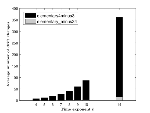
Figure 1. Average number of drift changes for $\xi=1.4$: elementary4minus3 vs. elementary_minus34

3.4.2. Comparison of solution sample paths

Figure 2 shows 100 sample paths of the numerical reference solution ($\Delta=2^{-14}$). The black line represents the discontinuity in the drift coefficient.

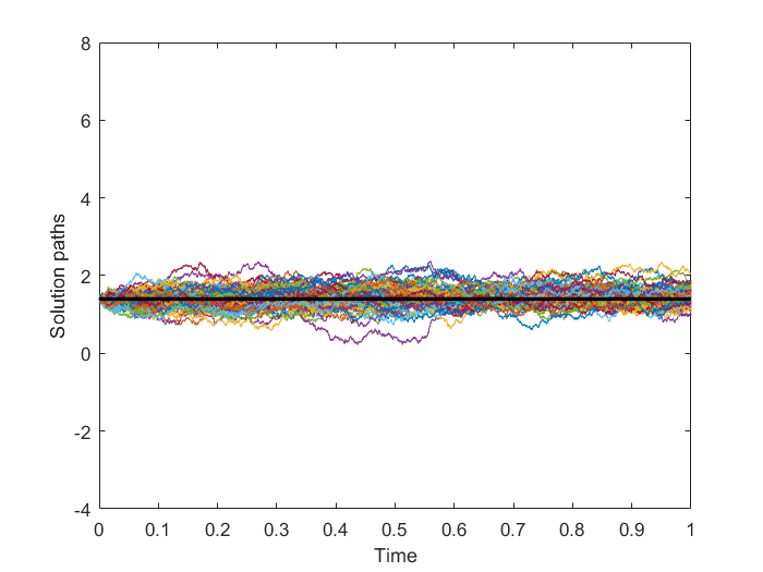
(a)  elementary4minus3, $\xi=1.4$

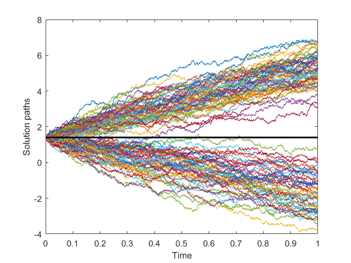
(b)  elementary_minus34, $\xi=1.4$

Figure 2. Comparison of solution paths: elementary4minus3 vs. elementary_minus34

In the situation of Figure 2(b), where the solution drifts away from the discontinuity, it is of tremendous importance whether a drift change is captured by the approximation or not: the solution does not stay close to the discontinuity and thus, there are not many chances for a drift correction to take place, see Figure 3. For the SDE

(14) $$dX_{t}=\left(\alpha_{1}\cdot\mathbbmss{1}_{(-\infty,0)}(X_{t})+\alpha_{2}\cdot\mathbbmss{1}_{[0,\infty)}(X_{t})\right)dt+dW_{t},\quad t\geq 0,\qquad X_{0}=\xi,$$

with $\alpha_{1}<0<\alpha_{2}$ and $\xi>0$ the conditional probability $p(\xi,\theta,\Delta)$ that the exact solution changes its drift over $[0,\Delta]$ given that the approximation $x_{1}$ at $t=\Delta$ has value $\theta\geq 0$ (and thus has not changed its drift) satisfies

(15) $$p(\xi,\theta,\Delta):=\mathbb{P}\Big{(}\inf_{t\in[0,\Delta]}X_{t}<0\Big{|}X_{0}=\xi,x_{1}=\theta\Big{)}=\exp\left(-2\frac{\xi\theta}{\Delta}\right),$$

see e.g. [10], page 169. So the (conditional) probability of missing drift changes is not negligible and even close to one for small $\xi$ or $\theta$.

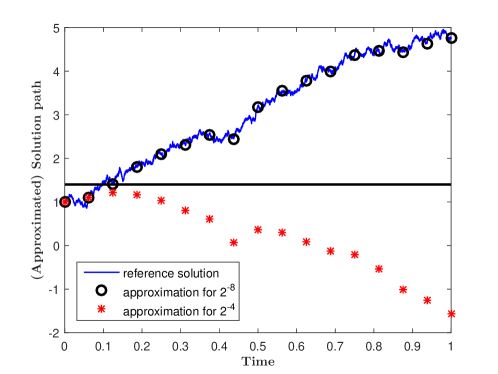
Figure 3. Importance of capturing the drift changes for elementary_minus34, $\xi=1$

3.4.3. Largest error

The latter observation is also reflected in the largest distance for $10^{4}$ sample paths between the approximation based on step size $2^{-10}$ and the numerical reference solution, see Table 5. The largest distances amount to 1.271 for elementary4minus3 and 4.508 for elementary_minus34.

Table 5. Largest and smallest Euler errors

Initial values		0	1	1.2	1.25	1.4	2
elementary_minus34	max	0.045	1.331	2.614	3.087	4.508	0.335
	min	0.0002	0.179	0.331	0.383	0.696	0.059
elementary4minus3	max	1.223	0.934	0.968	0.981	1.013	1.271
	min	0.005	0.005	0.005	0.005	0.005	0.005

3.4.4. Evolution of the error over time

To gain even more insight, we compare the empirical RMSE for increasing time $t$ of elementary4minus3 and elementary_minus34 when starting in the discontinuity $\xi=1.4$ for step sizes $2^{-4}$, $2^{-8}$ and $2^{-10}$ by plotting the base-2 logarithm of the RMSE against the time (see Figure 4). We have added in these figures the following additional information: If the number is not zero, the most frequent times of drift changes corresponding to the chosen step size are indicated. The number of plotted drift change times is based on the average number of drift changes over the simulated sample paths.

Furthermore, if in the corresponding cases drift changes occur, we add the very first drift change (of all simulated paths) of the numerical reference solution and the Euler schemes. They are generated by finding the time at which the first drift change occurs for $10^{4}$ saved paths and then taking the minimum over all that times. The time is registered as the point of discretization at which a drift change that took place was detected. The very first drift change of the reference solution is marked at a height of zero for a better distinguishability. RMSE over time and drift change times are calculated on a basis of $10^{4}$ simulation paths.

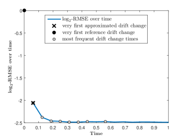
(a)  elementary4minus3, $\tilde{n}=4$

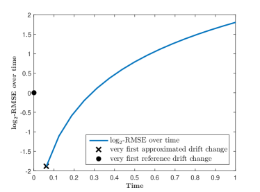
(b)  elementary_minus34, $\tilde{n}=4$

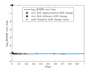
(c)  elementary4minus3, $\tilde{n}=8$

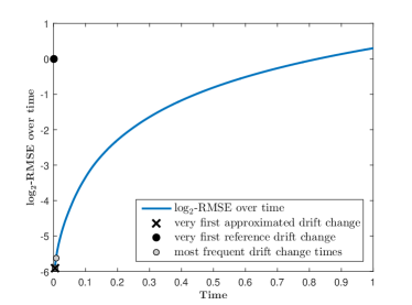
(d)  elementary_minus34, $\tilde{n}=8$

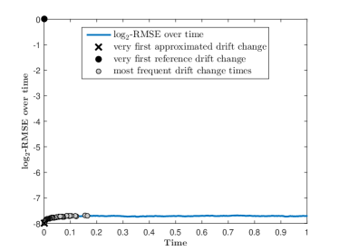
(e)  elementary4minus3, $\tilde{n}=10$

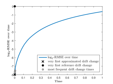
(f)  elementary_minus34, $\tilde{n}=10$

Figure 4. Comparison of the error evolution over time for $\xi=1.4$ for different step sizes: elementary4minus3 vs. elementary_minus34

We can extract from Figure 4 at least two features:

• The error stays constant or even decreases over time for elementary4minus3 – in contrast to a strong error accumulation over time for elementary_minus34. (Note that the ordinate has a base-2 log scale.)

• In the inward pointing drift coefficient case, the error is by several magnitudes smaller than for an outward pointing drift coefficient.

This illustrates again the stabilizing effect of an inward pointing drift coefficient and the importance of capturing the first drift changes correctly in case of an outward pointing drift coefficient.

3.4.5. Distribution of error sizes

Besides the empirical RMSE itself, the empirical distribution of the errors in $t=T$ is of interest. The error at final time $T$ is quantified by $\left|x_{N}-x_{n}\right|$ for step size $\Delta=T/n=2^{-\tilde{n}}$. The histograms in Figure 5 are based on $M=10^{4}$ simulations for different step sizes and highlight again the different magnitudes of the empirical RMSE (abscissa with a base-$2$ logarithm scale). Another feature, which we can extract from the histograms, is a non-negligible part of simulated paths with an error of machine accuracy size for elementary_minus34. We will discuss this feature in more detail in the next Subsection.

(a)  elementary4minus3

(b)  elementary_minus34

Figure 5. Distribution of the error at time $T$ for different step sizes for elementary4minus3 and elementary_minus34 with $\xi=1.4$

3.5. Rare events and goodness of the regression fit

In case of an outward pointing drift coefficient the empirical RMSE and the linear regression estimates become unreliable or at least questionable.

For initial values close to the discontinuity the observed empirical convergence order are in some cases far away from the guarenteed $3/4$, altough the linear regression typically produces stable results, see Figure 6(b). A possible explanation for this are again the first drift changes. When starting close to the initial value, the first drift changes seem to be very sensitive to the step-size, which results in rather different trajectories of the Euler scheme.

Furthermore, if the initial value is far away from the discontinuity, only very few drift changes occur in the underlying SDE (if at all). Hence, if the step size of the Euler scheme is significantly small, these changes are captured and the error drops drastically. Figure 6 illustrates this by comparing the regressions for an initial value $\xi=0$ away from the discontinuity in $1.4$ and an initial value $\xi=1$, which is closer to the discontinuity. (The regression has also to deal in Figure 6(a) with two different regimes.) Note that the Euler scheme for (1) is always exact up to the time of the first drift change.

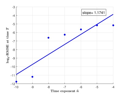
(a)  $\xi=0$

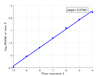
(b)  $\xi=1$

Figure 6. Euler rates of convergence for elementary_minus34 for $\xi\in\{0,1\}$

Moreover, for an outward pointing drift coefficient, the Euler scheme and the exact solution coincide with high probability, which explains e.g. the errors close to machine accuracy for the drift coefficient sign and the initial value $\xi=5$. Note that in this setting, the number of paths with at least one drift change is even zero over all saved $10^{4}$ solution paths.

To explain this phenomenon, consider again the SDE

(16) $$dX_{t}=\left(\alpha_{1}\cdot\mathbbmss{1}_{(-\infty,0)}(X_{t})+\alpha_{2}\cdot\mathbbmss{1}_{[0,\infty)}(X_{t})\right)dt+dW_{t},\quad t\geq 0,\qquad X_{0}=\xi,$$

with $\alpha_{1}<0<\alpha_{2}$. An application of formula (5.13) in chapter 3.5.C in [16] gives

(17) $$\mathbb{P}\left(\inf_{t\geq 0}|X_{t}|>0\right) =1-e^{2\alpha_{1}\xi^{-}-2\alpha_{2}\xi^{+}},\qquad\xi\neq 0.$$

Note that an initial value $\xi\neq 0$ is not a restriction as we analyze the case of an initial value far away from the discontinuity. So, for drift values $-\alpha_{1}=\alpha_{2}=1$, and an initial value $\xi=5$, the Euler scheme is exact with a probability of at least $1-e^{-10}$ $\approx 0.99995460\ldots$

To summarize: Standard Monte Carlo simulations for testing convergence rates seem to be unreliable in the case of outward pointing coefficients. No stable asymptotic regime seems to be reached by our estimators. Smaller stepsizes or a larger Monte-Carlo sample might be a remedy for this problem, similar to [13] where moment explosions of the Euler scheme for SDEs with superlinear cofficients are observed in a numerically asymptotic setting. But this is beyond the scope of the present manuscript.

4. The Euler scheme for the Atlas model

In this section, we will use the Euler scheme to simulate the so-called Atlas model, which is a particular first-order market model [4]. In such models, the asset dynamics depend on the size (measured in terms of market capitalization) of the corresponding firm, which results in an SDE model with discontinuous coefficients.

4.1. First-order market models

A first-order model [4] is defined as follows: Let $\gamma,g_{1},...,g_{d}\in\mathbb{R}$ and $\sigma_{1},...,\sigma_{d}\in(0,\infty)$ such that

$$g_{1}<0,\quad g_{1}+g_{2}<0,\ldots,\quad g_{1}+\cdots+g_{d-1}<0,\quad g_{1}+\cdots+g_{d}=0.$$

Consider now stocks for which the market capitalizations are given by $X_{1},\ldots,X_{d}$, where the index $i\in\{1,2,\ldots,d\}$ indicates the name of the firm, and that follow the dynamics

(18) $$d\log X_{i}(t)=\gamma_{i}(t)dt+\sigma_{i}(t)dW_{i}(t),\quad t\in[0,\infty),\qquad i=1,\ldots,d.$$

Here, $W_{1},...,W_{d}$ are independent Brownian motions and the growth rates $\gamma_{i}:[0,\infty)\rightarrow\mathbb{R}$ and volatilities $\sigma_{i}:[0,\infty)\rightarrow(0,\infty)$ are given by

(19) $$\gamma_{i}(t) =\gamma+\sum_{k=1}^{d}g_{k}\mathbbmss{1}_{\{r_{i}(t)=k\}},\qquad\quad\sigma_{i}(t)=\sum_{k=1}^{d}\sigma_{k}\mathbbmss{1}_{\{r_{i}(t)=k\}}.$$

The ranks $r_{i}(t)$ for the stock $X_{i}(t)$ at time $t$ arise from the reverse order-statistics:

(20) $$\max_{1\leq i\leq d}X_{i}(t)\mathrel{=}{\mathop{:}}X_{(1)}(t)\geq X_{(2)}(t)\geq\cdots\geq X_{(d-1)}(t)\geq X_{(d)}(t)\mathrel{\mathop{:}}=\min_{1\leq i\leq d}X_{i}(t).$$

Ties in the ranking are resolved by giving the firm with a lower index $i$ the better ranking. So, in such a model the $k$-th largest firm is assigned a growth rate of $\gamma+g_{k}$ and a volatility of $\sigma_{k}$ over the whole time horizon.

According to [4], the simplest among the first-order models is the so-called Atlas model, which was introduced in [7, Ex. 5.3.3]. Within the setting of (18) and (19), choosing

(21) $$\gamma=g>0,\quad g_{k}=-g,\,\,k=1,\ldots,d-1,\quad g_{d}=(d-1)g\quad\text{and}\quad\sigma_{i}(t)=\sigma>0,\,\,i=1,\ldots,d,$$

leads to the Atlas model. Here, only the smallest stock in the market – called the Atlas stock – has a nonzero but positive growth rate (for its log-dynamics).

By setting $Y_{i}(t)\mathrel{\mathop{:}}=\log X_{i}(t)$, $i=1,...,d$, as well as plugging in the Atlas parameters (21) in our first-order model (18) – (19), we obtain the Atlas model in compact form as

(22) $$dY_{i}(t) =(d\cdot g)\mathbbmss{1}_{\{r_{i}(t)=d\}}dt+\sigma dW_{i}(t),\quad i=1,...,d.$$

As stated in [4, Prop. 2.3], the solution of (22) satisfies the ergodic relation

(23) $$\lim\limits_{T\rightarrow\infty}\frac{1}{T}\int_{0}^{T}\mathbbmss{1}_{\{r_{i}(t)=k\}}dt=\frac{1}{d}\quad\textrm{a.s.},\qquad i,k=1,\ldots,d,$$

i.e., all stocks in the market asymptotically spent at each rank approximately the same amount of time. Similar ergodic relations also hold for general first-order market models.

4.2. Numerical results

For simulations of the Atlas and general first-order models one has to rely on discretization schemes such as the Euler method. In this subsection, we test whether the Euler scheme is able to recover the long time behavior (23), i.e., whether the discrete occupation rates

$$\frac{1}{T}\sum_{\ell=1}^{T/\Delta}\mathbbmss{1}_{\{\widehat{r}_{i}(\ell\Delta)=k\}},\qquad i,k=1,\ldots,d,$$

where $\widehat{r}_{i}$ is the discretized counterpart of (20) based on the Euler scheme and $T/\Delta\in\mathbb{N}$, converge to the analytical value.

Here, we consider a three-dimensional model with initial log-capitalizations ${Y(0)=[3.4,4.1,5.7]}$ and $\widetilde{Y}(0)=[1.2,3.5,10.8]$, $\gamma=0.1$ as market drift and $\sigma=0.09$ as market volatility. Table 6 presents the discrete occupation rates (averaged over $M=10^{3}$ repetitions) for $\Delta=2^{-14}$ and different values of $T$ as well as the sum of the squared deviations from the analytical asymptotic occupation rate. As hoped, the discrete occupation rates converge to the analytical asymptotic occupation rate of $1/d=1/3$ with increasing time horizon.

Furthermore, results suggest that less varying initial capitalizations imply that the numerical values are closer to the analytical result already for shorter time horizons, which coincides with the intuitive understanding. We also simulated the above scenarios with $\Delta=2^{-10}$ instead of $\Delta=2^{-14}$: all occupation times where equal with an accuracy of four digits and one third of the $90$ occupation rates differed in the fifth digit. This suggests that – as soon as the step size is small enough – a further refinement of the step size is no longer beneficial and the crucial simulation parameter is $T$, the endpoint of the considered time horizon.

Table 6. Discrete occupation rates for the discretized Atlas model

	T		Firm 1	Firm 2	Firm 3	Quadratic deviations
$Y(0)$	100	Rank 1	0.2911	0.2895	0.4194	0.0030	0.0031	0.0111
		Rank 2	0.3425	0.3662	0.2913
		Rank 3	0.3664	0.3443	0.2892
	250	Rank 1	0.3156	0.3161	0.3683	0.0005	0.0005	0.0018
		Rank 2	0.3375	0.3463	0.3162
		Rank 3	0.3469	0.3376	0.3155
	500	Rank 1	0.3238	0.3246	0.3517	0.0001	0.0001	0.0005
		Rank 2	0.3357	0.3400	0.3243
		Rank 3	0.3406	0.3354	0.3240
	750	Rank 1	0.3273	0.3273	0.3454	0.0001	0.0001	0.0002
		Rank 2	0.3347	0.3379	0.3274
		Rank 3	0.3380	0.3348	0.3272
	1000	Rank 1	0.3288	0.3287	0.3425	0.0000	0.0000	0.0001
		Rank 2	0.3344	0.3368	0.3288
		Rank 3	0.3368	0.3345	0.3287
	T		Firm 1	Firm 2	Firm 3	Quadratic deviations
$\widetilde{Y}(0)$	100	Rank 1	0.1464	0.1447	0.7089	0.0554	0.0562	0.2116
		Rank 2	0.3883	0.4654	0.1463
		Rank 3	0.4653	0.3899	0.1448
	250	Rank 1	0.2581	0.2579	0.4840	0.0090	0.0090	0.0341
		Rank 2	0.3555	0.3863	0.2582
		Rank 3	0.3864	0.3558	0.2577
	500	Rank 1	0.2949	0.2956	0.4096	0.0023	0.0023	0.0087
		Rank 2	0.3448	0.3599	0.2953
		Rank 3	0.3603	0.3446	0.2951
	750	Rank 1	0.3082	0.3079	0.3840	0.0010	0.0010	0.0038
		Rank 2	0.3407	0.3513	0.3081
		Rank 3	0.3511	0.3409	0.3080
	1000	Rank 1	0.3143	0.3142	0.3715	0.0006	0.0006	0.0022
		Rank 2	0.3391	0.3467	0.3143
		Rank 3	0.3467	0.3391	0.3143

5. Conclusion and Outlook

We have seen that the numerical approximation of solutions of SDEs with discontinuous drift coefficients is a challenging task, where several particularities arise. We were able to identify two main classes of discontinuous drift coefficients: outward and inward pointing drift coefficients. For the latter class, we analyzed stability properties. It turned out that the main difficulty in measuring the empirical convergence rates is how to appropriately capture drift changes. For inward pointing coefficients, we obtained stable estimates, which are in accordance with the theoretical results. For outward pointing cases, the estimates seem to be unreliable, no stabilizing asymptotic regime seems to be reached for the estimates. We tested two higher-order numerical schemes, that are frequently used in a setting where coefficients are sufficiently smooth. However, both schemes did not lead to an improved behavior.

References

- [1] A. Alfonsi, Strong order one convergence of a drift implicit Euler scheme: application to the CIR process, Stat. Probab. Lett., 83 (2013), pp. 602–607.
- [2] S. Asmussen and M. Taksar, Controlled diffusion models for optimal dividend pay-out, Insurance: Mathematics and Economics, 20 (1997), pp. 1–15.
- [3] A. V. Balakrishnan, On stochastic bang bang control, Applied Mathematics and Optimization, 6 (1980), pp. 91–96.
- [4] A. D. Banner, R. Fernholz, and I. Karatzas, Atlas models of equity markets, The Annals of Applied Probability, 15 (2005), pp. 2296–2330.
- [5] J. B. Detemple, R. Garcia, and M. Rindisbacher, A Monte Carlo method for optimal portfolios, The Journal of Finance, 58 (2003), pp. 401–446.
- [6] A. Eberle, Markov Processes, Lecture notes, University of Bonn, 2016.
- [7] E. R. Fernholz, Stochastic Portfolio Theory, vol. 48 of Applications of Mathematics, Stochastic Modelling and Applied Probability, Springer, New York, 2002.
- [8] R. Fernholz, T. Ichiba, and I. Karatzas, A second-order stock market model, Ann. Finance, 9 (2013), pp. 439–454.
- [9] I. Gihman and A. Skorohod, Stochastic differential equations, Springer, Berlin, Heidelberg, New York, 1972.
- [10] E. Gobet, Weak approximation of killed diffusion using Euler schemes, Stochastic Processes and their Applications, 87 (2000), pp. 167 – 197.
- [11] I. Gyöngy, A note on Euler’s approximations, Potential Analysis, 8 (1998), pp. 205–216.
- [12] N. Halidias and P. E. Kloeden, A note on the Euler–Maruyama scheme for stochastic differential equations with a discontinuous monotone drift coefficient, BIT Numerical Mathematics, 48 (2008), pp. 51–59.
- [13] M. Hutzenthaler, A. Jentzen, and P. E. Kloeden, Strong and weak divergence in finite time of Euler’s method for stochastic differential equations with non-globally Lipschitz continuous coefficients, Proc. R. Soc. Lond. Ser. A Math. Phys. Eng. Sci., 467 (2011), pp. 1563–1576.
- [14] T. Ichiba, V. Papathanakos, A. Banner, I. Karatzas, and R. Fernholz, Hybrid Atlas models, The Annals of Applied Probability, 21 (2011), pp. 609–644.
- [15] I. Karatzas and R. Fernholz, Stochastic portfolio theory: an overview, Handbook of numerical analysis, 15 (2009), pp. 89–167.
- [16] I. Karatzas and S. E. Shreve, Brownian motion and stochastic calculus, Springer, New York, Berlin, Heidelberg, 1991.
- [17] M. L. Kleptsyna and A. Y. Veretennikov, On strong solutions of stochastic Itô-Volterra equations, Theory of Probability & its Applications, 29 (1985), pp. 153–157.
- [18] P. E. Kloeden and E. Platen, Numerical Solution of Stochastic Differential Equations, vol. 23, Springer, Berlin, Heidelberg [u.a.], corr. 3. print ed., 1999.
- [19] A. Kohatsu-Higa, A. Lejay, and K. Yasuda, On Weak Approximation of Stochastic Differential Equations with Discontinuous Drift Coefficient, in Mathematical Economics, C. Hara, ed., vol. 1788, Kyoto, Japan, 2011, pp. 94–106.
- [20] H. J. Kushner and P. Dupuis, Numerical methods for stochastic control problems in continuous time, vol. 24 of Applications of Mathematics (New York), Springer, New York, second ed., 2001. Stochastic Modelling and Applied Probability.
- [21] E. M. LaBolle, J. Quastel, G. E. Fogg, and J. Gravner, Diffusion processes in composite porous media and their numerical integration by random walks: Generalized stochastic differential equations with discontinuous coefficients, Water Resources Research, 36 (2000), pp. 651–662.
- [22] G. Leobacher, M. Szölgyenyi, and S. Thonhauser, On the existence of solutions of a class of sdes with discontinuous drift and singular diffusion, Electron. Commun. Probab., 20 (2015), p. 14 pp.
- [23] G. Leobacher and M. Szölgyenyi, Convergence of the Euler–Maruyama method for multidimensional SDEs with discontinuous drift and degenerate diffusion coefficient, arXiv preprint, arXiv:1610.07047, (2016).
- [24] , A numerical method for SDEs with discontinuous drift, BIT, 56 (2016), pp. 151–162.
- [25] , A Strong Order 1/2 Method for Multidimensional SDEs with Discontinuous Drift, Annals of Applied Probability, (to appear).
- [26] J. Mattingly, A. Stuart, and D. Higham, Ergodicity for SDEs and approximations: locally Lipschitz vector fields and degenerate noise, Stochastic Processes Appl., 101 (2002), pp. 185–232.
- [27] S. Meyn and R. Tweedie, Markov chains and stochastic stability, Springer, Berlin, 1993.
- [28] T. Müller-Gronbach and L. Yaroslavtseva, On the performance of the Euler-Maruyama scheme for SDEs with discontinuous drift coefficient, arXiv e-prints, (2018), p. arXiv:1809.08423.
- [29] A. Neuenkirch and M. Szölgyenyi, The Euler-Maruyama scheme for SDEs with irregular drift: convergence rates via reduction to a quadrature problem, in preparation, (2019).
- [30] A. Neuenkirch, M. Szölgyenyi, and L. Szpruch, An adaptive Euler-Maruyama scheme for stochastic differential equations with discontinuous drift and its convergence analysis, arXiv e-prints, (2018), p. arXiv:1802.04521.
- [31] A. Neuenkirch and L. Szpruch, First order strong approximations of scalar SDEs defined in a domain, Numer. Math., 128 (2014), pp. 103–136.
- [32] H.-L. Ngo and D. Taguchi, Strong rate of convergence for the Euler–Maruyama approximation of stochastic differential equations with irregular coefficients, Math. Comput., 85 (2016), pp. 1793–1819.
- [33] H.-L. Ngo and D. Taguchi, On the Euler–Maruyama approximation for one-dimensional stochastic differential equations with irregular coefficients, IMA Journal of Numerical Analysis, (2017).
- [34] , Strong convergence for the Euler–Maruyama approximation of stochastic differential equations with discontinuous coefficients, Statist. Probab. Lett., 125 (2017), pp. 55–63.
- [35] M. M. Olama, S. M. Djouadi, and C. D. Charalambous, Stochastic differential equations for modeling, estimation and identification of mobile-to-mobile communication channels, IEEE Transactions on Wireless Communications, 8 (2009), pp. 1754–1763.
- [36] G. O. Roberts and R. L. Tweedie, Exponential convergence of Langevin distributions and their discrete approximations, Bernoulli, 2 (1996), pp. 341–363.
- [37] A. A. SHARDIN and M. SZÖLGYENYI, Optimal control of an energy storage facility under a changing economic environment and partial information, International Journal of Theoretical and Applied Finance, 19 (2016), p. 1650026.
- [38] M. Simonsen, J. Leth, H. Schiøler, and H. D. Cornean, A simple stochastic differential equation with discontinuous drift, in Proceedings Third International Workshop on Hybrid Autonomous Systems, HAS 2013, Rome, Italy, 17th March 2013., 2013, pp. 109–123.
- [39] M. Simonsen, H. Schioler, J. Leth, and H. Cornean, A convergence result for the Euler-Maruyama method for a simple stochastic differential equation with discontinuous drift, in 2014 American Control Conference, June 2014, pp. 5180–5185.
- [40] N. Touzi, Optimal stochastic control, stochastic target problems, and backward SDE, vol. 29 of Fields Institute Monographs, Springer, New York; Fields Institute for Research in Mathematical Sciences, Toronto, ON, 2013. With Chapter 13 by Angès Tourin.
- [41] A. J. Veretennikov, On strong solutions and explicit formulas for solutions of stochastic integral equations, Mathematics of the USSR-Sbornik, 39 (1981), pp. 387–403.
- [42] Zvonkin, A. K., A transformation of the phase space of a diffusion process that removes the drift, Mathematics of the USSR-Sbornik, 22 (1974), pp. 129–149.