Formalizing Timing Diagram Requirements in Discrete Duration Calulus

Abstract

Several temporal logics have been proposed to formalise timing diagram requirements over hardware and embedded controllers. These include LTL [CF05], discrete time MTL [AH93] and the recent industry standard PSL [EF16]. However, succintness and visual structure of a timing diagram are not adequately captured by their formulae [CF05]. Interval temporal logic QDDC is a highly succint and visual notation for specifying patterns of behaviours [Pan00].

In this paper, we propose a practically useful notation called SeCeNL which enhances negation free fragment of QDDC with features of nominals and limited liveness. We show that timing diagrams can be naturally (compositionally) and succintly formalized in SeCeNL as compared with PSL-Sugar and MTL. We give a linear time translation from timing diagrams to SeCeNL. As our second main result, we propose a linear time translation of SeCeNL into QDDC. This allows QDDC tools such as DCVALID [Pan00, Pan01] and DCSynth to be used for checking consistency of timing diagram requirements as well as for automatic synthesis of property monitors and controllers. We give examples of a minepump controller and a bus arbiter to illustrate our tools. Giving a theoretical analysis, we show that for the proposed SeCeNL, the satisfiability and model checking have elementary complexity as compared to the non-elementary complexity for the full logic QDDC.

1 Introduction

A timing diagram is a collection of binary signals and a set of timing constraints on them. It is a widely used visual formalism in the realm of digital hardware design, communication protocol specification and embedded controller specification. The advantages of timing diagrams in hardware design are twofold, one, since designers can visualize waveforms of signals they are easy to comprehend and two, they are very convenient for specifying ordering and timing constraints between events (see figures Fig. 1 and Fig. 2 below).

There have been numerous attempts at formalizing timing diagram constraints in the framework of temporal logics such as the timing diagram logic [Fis99], with LTL formulas [CF05], and as synchronous regular timing diagrams [AEKN00]. Moreover, there are industry standard property specification languages such as PSL/Sugar and OVA for associating temporal assertions to hardware designs [EF16]. The main motivation for these attempts was to exploit automatic verification techniques that these formalisms support for validation and automatic circuit synthesis. However, commenting on their success, Fisler et. al. state that the less than satisfactory adoption of formal methods in timing diagram domain can be partly attributed to the gulf that exists between graphical timing diagrams and textual temporal logic – expressing various timing dependencies that can exist among signals that can be illustrated so naturally in timing diagrams is rather tedious in temporal logics [CF05]. As a result, hardware designers use timing diagrams informally without any well defined semantics which make them unamenable to automatic design verification techniques.

In this paper, we take a fresh look at formalizing timing diagram requirements with emphasis on the following three features of the formalism that we propose here.

Firstly, we propose the use of an interval temporal logic QDDC to specify patterns of behaviours. QDDC is a highly succinct and visual notation for specifying regular patterns of behaviours [Pan00, Pan01, KP05]. We identify a quantifier and negation-free subset SeCe of QDDC which is sufficient for formalizing timing diagram patterns. It includes generalized regular expression like syntax with counting constructs. Constraints imposed by timing diagrams are straightforwardly and compactly stated in this logic. For example, the timing diagram in Fig. 1 stating that $P$ transits from 0 to 1 somewhere in interval $u$ to $u+3$ cycles is captured by the SeCe formula [$\neg$ P]^<u>^(slen=3 $\wedge$ [$\neg$P]^[[P]])^[[P]]. The main advantage of SeCe is that it has elementary satisfiability as compared to the non-elementary satisfiability of general QDDC.

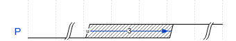
Figure 1: Timing diagram with a marked position $u$ and a timing constraint.

Secondly, it is very typical for timing diagrams to have partial ordering and synchronization constraints between distinct events. Emphasizing this aspect, formalisms such as two dimensional regular expressions [Fis07] have been proposed for timing diagrams. We find that synchronization in timing diagram may even extend across different patterns of limited liveness properties. In order to handle such synchronization, we extend our logic SeCe with nominals from hybrid temporal logics [FdRS03]. Nominals are temporal variables which “freeze” the positions of occurrences of events. They naturally allow synchronization across formulae.

Thirdly, we enhance the timing diagram specifications (as well as logic SeCe) with limited liveness operators. While timing diagrams visually specify patterns of occurrence of signals, they do not make precise the modalities of occurrences of such patterns. We explicitly introduce modalities such as a) initially, a specified pattern must occur, or that b) every occurrence of pattern1 is necessarily and immediately followed by an occurrence of pattern2, or that c) occurrence of a specified pattern is forbidden anywhere within a behaviour. In this, we are inspired by Allen’s Interval Algebra relations [All83] as well as the LSC operators of Harel for message sequence charts [DH01]. We confine ourselves to limited liveness properties where good things are achieved within specified bounds. For example, in specifying a modulo 6 counter, we can say that the counter will stabilize before completion of first 15 cycles. Astute readers will notice that, technically, our limited liveness operators only give rise to “safety” properties (in the sense of Alpern and Schneider [AS87]). However, from a designer’s perspective they do achieve the practical goal of forcing good things to happen.

Putting all these together, we define a logic SeCeNL which includes negation-free QDDC together with limited liveness operators as well as nominals. The formal syntax and semantics of SeCeNL formulas is given in §2.3. We claim that SeCeNL provides a natural and convenient formalism for encoding timing diagram requirements. Substantiating this, we formulate a translation of timing diagrams into SeCeNL formulae in §3. The translation is succinct, in fact, linear time computable in the size of the timing diagram. (A textual syntax is used for timing diagrams. The textual syntax of timing diagrams used is inspired by the tool WaveDrom [CP16], which is also used for graphical rendering of our timing diagram specifications.) Moreover, the translation is compositional, i.e. it translates each element of the timing diagram as one small formula and overall specification is just the conjunction of such constraints. Hence, the translation preserves the structure of the diagram.

With several examples of timing diagrams, we compare its SeCeNL formula with the formula in logics such as PSL-Sugar and MTL. Logic PSL-Sugar is amongst the most expressive notations for requirements. Logic PSL-Sugar is syntactically a superset of MTL and LTL. It extends LTL with SERE (regular expressions with intersection) which are similar to our SeCe. In spite of this, we a show natural examples where SeCeNL formula is at least one exponent more succinct as compared to PSL-Sugar.

As the second main contribution of this paper, we consider formal verification and controller synthesis from SeCeNL specifications. In §3.1, we formulate a reduction from a SeCeNL formula to an equivalent QDDC formula. This allows QDDC tools to be used for SeCeNL. It may be noted that, though expressively no more powerful than QDDC, logic SeCeNL considerably more efficient for satisfiability and model checking. We show that these problems have elementary complexity as compared with full QDDC which exhibits non-elementary complexity. Also, the presence of limited liveness and nominals makes it more convenient as compared to QDDC for practical use.

By implementing the above reductions, we have constructed a Python based translator which converts a requirement consisting of a boolean combination of timing diagram specifications (augmented with limited liveness) and SeCeNL formulae into an equivalent QDDC formula. We can analyze the resulting formula using the QDDC tools DCVALID [Pan00, Pan01] as well as DCSynthG for model checking and controller synthesis, respectively (see Fig. 11 for the tool chain). We illustrate the use of our tools by the case studies of a synchronous bus arbiter and a minepump controller in §4. Readers may note that we specify rather rich quantitative requirements not commonly considered, and our tools are able to automatically synthesize monitors and controllers for such specifications.

2 Logic QDDC

Let $\Sigma$ be a finite non empty set of propositional variables. A word $\sigma$ over $\Sigma$ is a finite sequence of the form $P_{0}\cdots P_{n}$ where $P_{i}\subseteq\Sigma$ for each $i\in\{0,\ldots,n\}$. Let $len(\sigma)=n+1$, $dom(\sigma)=\{0,\ldots,n\}$ and $\forall i\in dom(\sigma):\sigma(i)=P_{i}$.

The syntax of a propositional formula over $\Sigma$ is given by:

$$\varphi:=\textsf{0}\ |\ \textsf{1}\ |\ p\in\Sigma\ |\ \varphi\wedge\varphi\ |\ \varphi\vee\varphi\ |\ \neg\varphi,$$

and operators such as $\Rightarrow$ and $\Leftrightarrow$ are defined as usual. Let $\Omega_{\Sigma}$ be the set of all propositional formulas over $\Sigma$.

Let $\sigma=P_{0}\cdots P_{n}$ be a word and $\varphi\in\Omega_{\Sigma}$. Then, for an $i\in dom(\sigma)$ the satisfaction relation $\sigma,i\models\varphi$ is defined inductively as expected: $\sigma,i\models\textsf{1}$; $\sigma,i\models p$ iff $p\in\sigma(i)$; $\sigma,i\models\neg p$ iff $\sigma,i\not\models p$, and the satisfaction relation for the rest of the boolean combinations defined in a natural way.

The syntax of a QDDC formula over $\Sigma$ is given by:

$$\begin{array}[]{lc}D:=&\langle\varphi\rangle\ |\ [\varphi]\ |\ [[\varphi]]\ |\ \{\{\varphi\}\}\ |\ D\ \verb|^|\ D\ |\ \neg D\ |\ D\vee D\ |\ D\wedge D\ |\ D^{*}\ |\vspace{1mm}\\ &\exists p.\ D\ |\ \forall p.\ D\ |\ slen\bowtie c\ |\ scount\ \varphi\bowtie c\ |\ sdur\ \varphi\bowtie c,\end{array}$$

where $\varphi\in\Omega_{\Sigma}$, $p\in\Sigma$, $c\in\mathbb{N}$ and $\bowtie\in\{<,\leq,=,\geq,>\}$.

An interval over a word $\sigma$ is of the form $[b,e]$ where $b,e\in dom(\sigma)$ and $b\leq e$. An interval $[b_{1},e_{1}]$ is a sub interval of $[b,e]$ if $b\leq b_{1}$ and $e_{1}\leq e$. Let $Intv(\sigma)$ be the set of all intervals over $\sigma$.

Let $\sigma$ be a word over $\Sigma$ and let $[b,e]\in Intv(\sigma)$ be an interval. Then the satisfaction relation of a QDDC formula $D$ over $\Sigma$, written $\sigma,[b,e]\models D$, is defined inductively as follows:

$$\begin{array}[]{lcl}\sigma,[b,e]\models\langle\varphi\rangle&\mathrm{\ iff\ }&\sigma,b\models\varphi,\\ \sigma,[b,e]\models[\varphi]&\mathrm{\ iff\ }&\forall b\leq i<e:\sigma,i\models\varphi,\\ \sigma,[b,e]\models[[\varphi]]&\mathrm{\ iff\ }&\forall b\leq i\leq e:\sigma,i\models\varphi,\\ \sigma,[b,e]\models\{\{\varphi\}\}&\mathrm{\ iff\ }&e=b+1\mbox{ and }\sigma,b\models\varphi,\\ \sigma,[b,e]\models\neg D&\mathrm{\ iff\ }&\sigma,[b,e]\not\models D,\\ \sigma,[b,e]\models D_{1}\vee D_{2}&\mathrm{\ iff\ }&\sigma,[b,e]\models D_{1}\mbox{ or }\sigma,[b,e]\models D_{2},\\ \sigma,[b,e]\models D_{1}\wedge D_{2}&\mathrm{\ iff\ }&\sigma,[b,e]\models D_{1}\mbox{ and }\sigma,[b,e]\models D_{2},\\ \sigma,[b,e]\models D_{1}\verb|^|D_{2}&\mathrm{\ iff\ }&\exists b\leq i\leq e:\sigma,[b,i]\models D_{1}\mbox{ and }\sigma,[i,e]\models D_{2}.\\ \end{array}$$

We call word $\sigma^{\prime}$ a $p$-variant, $p\in\Sigma$, of a word $\sigma$ if $\forall i\in dom(\sigma),\forall q\neq p:\sigma^{\prime}(i)(q)=\sigma(i)(q)$. Then $\sigma,[b,e]\models\exists p.~{}D\Leftrightarrow\sigma^{\prime},[b,e]\models D$ for some $p$-variant $\sigma^{\prime}$ of $\sigma$ and, $\sigma,[b,e]\models\forall p.~{}D\Leftrightarrow\sigma,[b,e]\not\models\exists p.~{}\neg D$. We define $\sigma\models D$ iff $\sigma,[0,len(\sigma)]\models D$.

Example 1

Let $\Sigma=\{p,q\}$ and let $\sigma=P_{0}\cdots P_{7}$ be such that $\forall 0\leq i<7:P_{i}=\{p\}$ and $P_{7}=\{q\}$. Then $\sigma,[0,7]\models[p]$ but not $\sigma,[0,7]\models[[p]]$ as $p\not\in P_{7}$.

Example 2

Let $\Sigma=\{p,q,r\}$ and let $\sigma=P_{0}\cdots P_{10}$ be such that $\forall 0\leq i<4:P_{i}=\{p\}$, $\forall 4\leq i<8:P_{i}=\{p,q,r\}$ and $\forall 8\leq i\leq 10:P_{i}=\{q,r\}$. Then

$$\sigma,[0,10]\models[p]\verb|^|[[\neg p\wedge r]]$$

because for $i\in\{8,9,10\}$ the condition $\exists 0\leq i\leq 10:\sigma,[0,i]\models[p]\mbox{ and }\sigma,[i,10]\models[[\neg p\wedge r]]$ is met. But $\sigma,[0,7]\not\models[p]\verb|^|[[\neg p\wedge r]]$ as $\neg\exists 0\leq i\leq 7:\sigma,[0,i]\models[p]\mbox{ and }\sigma,[i,7]\models[[\neg p\wedge r]]$.

Entities $slen$, $scount$, and $sdur$ are called terms in QDDC. The term $slen$ gives the length of the interval in which it is measured, $scount\ \varphi$ where $\varphi\in\Omega_{\Sigma}$, counts the number of positions including the last point in the interval under consideration where $\varphi$ holds, and $sdur\ \varphi$ gives the number of positions excluding the last point in the interval where $\varphi$ holds. Formally, for $\varphi\in\Omega_{\Sigma}$ we have $slen(\sigma,[b,e])=e-b$, $scount(\sigma,\varphi,[b,e])=\sum_{i=b}^{i=e}\left\{\begin{array}[]{ll}1,&\mbox{if }\sigma,i\models\varphi,\\ 0,&\mbox{otherwise.}\end{array}\right\}$ and $sdur(\sigma,\varphi,[b,e])=\sum_{i=b}^{i=e-1}\left\{\begin{array}[]{ll}1,&\mbox{if }\sigma,i\models\varphi,\\ 0,&\mbox{otherwise.}\end{array}\right\}$ In addition we also use the following derived constructs: $\sigma,[b,e]\models pt~{}$ iff $b=e$; $\sigma,[b,e]\models ext~{}$ iff $b<e$; $\sigma,[b,e]\models\Diamond D$ iff $true~{}\verb|^|D\verb|^|true~{}$ and $\sigma,[b,e]\models\Box D$ iff $\sigma,[b,e]\not\models\Diamond\neg D$.

A formula automaton for a QDDC formula $D$ is a deterministic finite state automaton which accepts precisely language $L=\{\sigma\ |\ \sigma\models D\}$.

Theorem 2.1

[Pan01] For every QDDC formula $D$ over $\Sigma$ we can construct a $DFA$ $\mathcal{A}(D)$ for $D$ such $\mathcal{L}(D)=\mathcal{L}(\mathcal{A}(D))$. The size of $\mathcal{A}(D)$ is non elementary in the size of $D$ in the worst case.

2.1 Chop expressions: Ce and SeCe

Definition 1

The logic Semi extended Chop expressions (SeCe) is a syntactic subset of QDDC in which the operators $\exists p.~{}D$, $\forall p.~{}D$ and negation are not allowed. The logic Chop expressions (Ce) is a sublogic of SeCe in which conjuction is not allowed.

Lemma 1

For any chop expression $D$ of size $n$ we can effectively construct a language equivalent $DFA$ $\mathcal{A}$ of size $\Omega(2^{2^{n}})$.

Proof

We observe that for any chop expression $D$ we can construct a language equivalent $NFA$ which is at most exponential in size of $D$ including the constants appearing in it (for a detailed proof see [BP12] wherein a similar result has been proved). But this implies there exists a $DFA$ of size $2^{2^{n}}$ which accepts exactly the set of words $\sigma$ such that $\sigma\models D$.

Corollary 1

For any SeCe $D$ of size $n$ we can effectively construct a language equivalent $DFA$ $\mathcal{A}$ of size $\Omega(2^{2^{2^{n}}})$.

Proof

Proof follows from the definition of SeCe, lemma 1 and from the fact that the size of the product of $DFA$’s can be atmost exponential in the size of individual $DFA$’s.

2.2 DCVALID and DCSynthG

The reduction from a QDDC formula to its formula automaton has been implemented into the tool DCVALID [Pan00, Pan01]. The formula automaton it generates is total, deterministic and minimal automaton for the formula. DCVALID can also translate the formula automaton into Lustre/SCADE, Esterel, SMV and Verilog observer module. By connecting this observer module to run synchronously with a system we can reduce model checking of QDDC property to reachability checking in observer augmented system. See [Pan00, Pan01] for details. A further use of formula automata can be seen in the tool called DCSynthG which synthesizes synchronous dataflow controller in SCADE/NuSMV/Verilog from QDDC specification.

2.3 Logic SeCeNL: Syntax and Semantics

We can now introduce our logic SeCeNL which builds upon SeCe by augmenting it with nominals and limited liveness operators.

Syntax

: The syntax of SeCeNL atomic formula is as follows. Let $D$, $D_{1}$, $D_{2}$ and $D_{3}$ range over SeCe formulae and let $\Theta$, $\Theta_{1}$, $\Theta_{2}$ and $\Theta_{3}$ range over subset of propositional variables occurring in SeCe formula. The notation $D:\Theta$, called a nominated formula, denotes that $\Theta$ is the set of variables used as nominals in the formula $D$.

$$\begin{array}[]{l}\mbox{{init}}(D_{1}:\Theta_{1}~{}/~{}D_{2}:\Theta_{2})~{}\mid~{}\mbox{{anti}}(D:\Theta)~{}\mid~{}\mbox{{pref}}(D:\Theta)~{}~{}\mid\\ \mbox{{implies}}(D_{1}:\Theta_{1}\leadsto D_{2}:\Theta_{2})~{}\mid~{}\mbox{{follows}}(D_{1}:\Theta_{1}\leadsto D_{2}:\Theta_{2}/D_{3}:\Theta_{3})~{}~{}\mid\\ \mbox{{triggers}}(D_{1}:\Theta_{1}\leadsto D_{2}:\Theta_{2}/D_{3}:\Theta_{3})\end{array}$$

An SeCeNL formula is a boolean combination of atomic SeCeNL formulae of the form above. As a convention, $D:\{\}$ is abbreviated as $D$ when the set of nominals $\Theta$ is empty.

2.3.1 Limited Liveness Operators

: Given an word $\sigma$ and a position $i\in dom(\sigma)$, we state that $\sigma,i\models D$ iff $\sigma[0:i]\models D$. Thus, the interpretation is that the past of the position $i$ in execution satisfies $D$.

For a SeCe formula $D$ we let $\Xi(D)=D\wedge\neg(D\verb|^|ext)$, which says that if $\sigma,[b,e]\models\Xi(D)$ then $\sigma,[b,e]\models D$ and there exists no proper prefix interval $[b,e_{1}]$, (i. e. $[b,e_{1}]\in Intv(\sigma)$ and $b\leq e_{1}<e$) such that $\sigma,[b,e_{1}]\models D$. We say $\sigma^{\prime}\leq_{prefix}\sigma$ if $\sigma^{\prime}$ is a prefix of $\sigma$, and $\sigma^{\prime}<_{prefix}\sigma$ if $\sigma^{\prime}$ is a proper prefix of $\sigma$.

We first explain the semantics of limited liveness operators assuming that no nominals are used in the specification, i.e. $\Theta$, $\Theta_{1}$, $\Theta_{2}$ and $\Theta_{3}$ are all empty. A set $S\subseteq\Sigma^{*}$ is prefix closed if $\sigma\in S$ then $\forall\sigma^{\prime}:\sigma^{\prime}\leq_{prefix}\sigma\Rightarrow\sigma^{\prime}\in S$. We observe that each atomic liveness formula denotes a prefix closed subset of $(2^{\Sigma})^{+}$.

• $L(\mbox{{pref}}(D)~{})=\{\sigma\ |\ \forall\sigma^{\prime}\leq_{prefix}\sigma:\sigma^{\prime}\models D\}.$ Operator $\mbox{{pref}}(D)~{}$ denotes that $D$ holds invariantly throughout the execution.

• $L(\mbox{{init}}(D_{1}/D_{2}))=\{\sigma\ |\ \forall j:\sigma,[0,j]\models D_{2}\Rightarrow\exists k\leq j:\sigma,[0,k]\models D_{1}\}.$ Operator $\mbox{{init}}(D_{1}/D_{2})$ basically states that if $j$ is the first position which satisfies $D_{2}$ in the execution then there exists an $i\leq j$ such that $i$ satisfies $D_{1}$. Thus, initially $D_{1}$ holds before $D_{2}$ unless the execution (is too short and hence) does not satisfy $D_{2}$ anywhere.

• $L(\mbox{{anti}}(D))=\{\sigma\ |\ \forall i,j:\sigma,[i,j]\not\models D\}$. Operator $\mbox{{anti}}(D)$ states that there is no observation sub interval of the execution which satisfies $D$.

• $L(\mbox{{implies}}(D_{1}\leadsto D_{2}))=\{\sigma\ |\ \forall i,j:(\sigma,[i,j]\models D_{1}\Rightarrow\sigma,[i,j]\models D_{2})\}$. Operator $\mbox{{implies}}(D_{1}\leadsto D_{2})$ states all observation intervals which satisfy $D_{1}$ will also satisfy $D_{2}$.

• $L(\mbox{{follows}}(D_{1}\leadsto D_{2}/D_{3}))=\{\sigma\ |\ \forall i,j:(\sigma,[i,j]\models D_{1}\Rightarrow$
                                   $(\forall k:\sigma,[j,k]\models\Xi(D_{3})\Rightarrow\exists l\leq k:\sigma,[j,l]\models D_{2}))\}.$
  Operator $\mbox{{follows}}(D_{1}\leadsto D_{2}/D_{3})$ states that if any observation interval $[i,j]$ satisfies $D_{1}$ and there is a following shortest interval $[j,k]$ which satisfies $D_{3}$ then there exists a prefix interval of $[j,k]$ which satisfies $D_{2}$.

• $L(\mbox{{triggers}}(D_{1}\leadsto D_{2}/D_{3}))=\{\sigma\ |\ \forall i,j:(\sigma,[i,j]\models D_{1}\Rightarrow$
                                    $(\forall k:\sigma,[i,k]\models\Xi(D_{3})\Rightarrow\exists l\leq k:\sigma,[i,l]\models D_{2}))\}.$
  Operator $\mbox{{triggers}}(D_{1}\leadsto D_{2}/D_{3})$ states that if any observation interval $[i,j]$ satisfies $D_{1}$ and if $[i,k]$ is the shortest interval which satisfies $D_{3}$ then $D_{2}$ holds for a prefix interval of $[i,k]$.

Based on this semantics, we can translate an atomic SeCeNL formula $\zeta$ without nominals into equivalent $SeCe$ formula $\aleph(\zeta)$ as follows.

1. $\aleph(\mbox{{pref}}(D)~{})\stackrel{{\scriptstyle\mathrm{def}}}{{\equiv}}\neg((\neg D)\verb|^|true~{})$.

2. $\aleph(\mbox{{init}}(D_{1}/D_{2}))\stackrel{{\scriptstyle\mathrm{def}}}{{\equiv}}pref(\Xi(D_{2})\Rightarrow D_{1}\verb|^|true~{})$.

3. $\aleph(\mbox{{anti}}(D))\stackrel{{\scriptstyle\mathrm{def}}}{{\equiv}}\neg(true~{}\verb|^|D\verb|^|true~{})$.

4. $\aleph(\mbox{{implies}}(D_{1}\leadsto D_{2}))\stackrel{{\scriptstyle\mathrm{def}}}{{\equiv}}\Box(D_{1}\Rightarrow D_{2})$.

5. $\aleph(\mbox{{follows}}(D_{1}\leadsto D_{2}/D_{3}))\stackrel{{\scriptstyle\mathrm{def}}}{{\equiv}}\Box(\neg(D_{1}\verb|^|(\Xi(D_{3})\wedge\neg(D_{2}\verb|^|true~{}))))$.

6. $\aleph(\mbox{{triggers}}(D_{1}\leadsto D_{2}/D_{3}))\stackrel{{\scriptstyle\mathrm{def}}}{{\equiv}}\Box(D_{1}\verb|^|true~{}\Rightarrow(\Xi(D_{3})\Rightarrow D_{2}\verb|^|true~{}))\bigwedge\Box(D_{1}\Rightarrow pref(\Xi(D_{3})\Rightarrow D_{2}\verb|^|true~{}))$.

Lemma 2

For any $\zeta\in SeCeNL$, if $\zeta$ does not use nominals then $\sigma\in L(\zeta)$ iff $\sigma\in L(\aleph(\zeta))$.

The proof follows from examination of the semantics of $\zeta$ and the definition of $\aleph(\zeta)$. We omit the details.

2.3.2 Nominals

: Consider a nominated formula $D:\Theta$ where $D$ is a SeCe formula over propositional variables $\Sigma\cup\Theta$. As we shall see later, the propositional variables in $\Theta$ are treated as “place holders” - variables which are meant to be true exactly at one point - and we call them nominals following [FdRS03].

Given an interval $[b,e]\in Intv(\mathbb{N})$ we define a nominal valuation over $[b,e]$ to be a map $\nu:\Theta\rightarrow\{i\ |\ b\leq i\leq e\}$. It assigns a unique position within $[b,e]$ to each nominal variable. We can then straightforwardly define $\sigma,[b,e]\models_{\nu}D$ by constructing a word $\sigma_{\nu}$ over $\Sigma\cup\Theta$ such that $\forall p\in\Sigma:p\in\sigma_{\nu}(i)\Leftrightarrow p\in\sigma(i)$ and $\forall u\in\Theta:u\in\sigma_{\nu}(i)\Leftrightarrow\nu(u)=i$. Then $\sigma_{\nu},[b,e]\models D\Leftrightarrow\sigma,[b,e]\models_{\nu}D$. We state that $\nu_{1}$ over $\Theta_{1}$ and $\nu_{2}$ over $\Theta_{2}$ are consistent if $\nu_{1}(u)=\nu_{2}(u)$ for all $u\in\Theta_{1}\cap\Theta_{2}$. We denote this by $\nu_{1}\parallel\nu_{2}$.

Semantics of SeCeNL

: Now we consider the semantics of SeCeNL where nominals are used and shared between different parts $D_{1}$, $D_{2}$ and $D_{3}$ of an atomic formula such as $\mbox{{implies}}(D_{1}:\Theta_{1}\leadsto D_{2}:\Theta_{2})$.

Example 3 (lags)

Let $D_{1}:\{u,v\}$ be the formula (<u> ^ [[P]] $\wedge$ ((slen=n) ^ <v> ^ true) which holds for an interval where $P$ is $true$ throughout the interval and $v$ marks the $n+1$ position from $u$ denoting the start of the interval. Let $D_{2}:\{v\}$ be the formula true ^ <v> ^ [[Q]]. Then, implies$(D_{1}:\{u,v\}\leadsto D_{2}:\{v\})$ states that for all observation intervals $[i,j]$ and all nominal valuations $\nu$ over $[i,j]$ if $\sigma,[i,j]\models_{\nu}D_{1}$ then $\sigma,[i,j]\models_{\nu}D_{2}$. This formula is given by live timing diagram in Fig. 2 below.

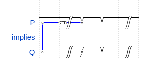
Figure 2: Live timing diagram.

We now give the semantics of SeCeNL.

• $L(\mbox{{pref}}(D:\Theta)~{})=\{\sigma\ |\ \forall\sigma^{\prime}\leq_{prefix}\sigma:\exists\nu.~{}~{}\sigma^{\prime}\models_{\nu}D\}.$

• $L(\mbox{{init}}(D_{1}:\Theta_{1}~{}/~{}D_{2}:\Theta_{2}))=\{\sigma~{}\mid~{}\forall j\forall\nu:\sigma,[0,j]\models_{\nu}D_{2}\Rightarrow\exists k\leq j\exists\nu_{2}:\nu_{1}\parallel\nu_{2}\land\sigma,[0,k]\models_{\nu_{2}}D_{1}\}.$

• $L(\mbox{{anti}}(D:\Theta))=\{\sigma\ |\ \forall i,j\forall\nu:\sigma,[i,j]\not\models_{\nu}D\}.$

• $L(\mbox{{implies}}(D_{1}:\Theta_{1}\leadsto D_{2}:\Theta_{2}))=\{\sigma\ |\ \forall i,j\forall\nu_{1}:(\sigma,[i,j]\models_{\nu_{1}}D_{1}\Rightarrow\exists\nu_{2}:\nu_{1}\parallel\nu_{2}\land\sigma,[i,j]\models_{\nu_{2}}D_{2})\}.$

• $L(\mbox{{follows}}(D_{1}:\Theta_{1}\leadsto D_{2}:\Theta_{2}/D_{3}:\Theta_{3}))=$
  $\{\sigma\ |\ \forall i,j\forall\nu_{1}:(\sigma,[i,j]\models_{\nu_{1}}D_{1}\Rightarrow(\forall k\forall\nu_{2}\parallel\nu_{1}:\sigma,[j,k]\models_{\nu_{2}}\Xi(D_{3})\Rightarrow\exists l\leq k\exists\nu_{3}:\nu_{3}\parallel\nu_{1}\land\nu_{3}\parallel\nu_{2}\land\sigma,[j,l]\models_{\nu_{3}}D_{2}))\}.$

• $L(\mbox{{triggers}}(D_{1}:\Theta_{1}\leadsto D_{2}:\Theta_{2}/D_{3}:\Theta_{3}))=$
            $\{\sigma\ |\ \forall i,j\forall\nu_{1}:(\sigma,[i,j]\models_{\nu_{1}}D_{1}\Rightarrow(\forall k\forall\nu_{2}\parallel\nu_{1}:\sigma,[i,k]\models_{\nu_{2}}\Xi(D_{3})\Rightarrow\exists l\leq k\exists\nu_{3}:\nu_{3}\parallel\nu_{1}\land\nu_{3}\parallel\nu_{2}\land\sigma,[i,l]\models D_{2}))\}.$

Based on the above semantics, we now formulate a QDDC formula equivalent to a SeCeNL formula. We define the following useful notations $\forall^{1}_{\Theta}:D$ and $\exists^{1}_{\Theta}:D$ as derived operators. These operators are essentially relativize quantifiers to restrict variables to singletons.

$$\begin{array}[]{c}\forall^{1}_{\Theta}:D\Leftrightarrow\forall u_{1}.\ \cdots\ .\forall u_{n}((scount\ u_{1}=1\ \wedge\cdots\wedge\ scount\ u_{n}=1)\ \Rightarrow\ D).\\ \exists^{1}_{\Theta}:D\Leftrightarrow\exists u_{1}.\ \cdots\ .\exists u_{n}((scount\ u_{1}=1\ \wedge\cdots\wedge\ scount\ u_{n}=1)\ \wedge\ D).\end{array}$$

From SeCeNL to QDDC

: We now define the translation $\aleph$ from SeCeNL to QDDC.

1. $\aleph(\mbox{{pref}}(D:\Theta)~{})\stackrel{{\scriptstyle\mathrm{def}}}{{\equiv}}\neg(\exists^{1}_{\Theta}:\neg D\verb|^|true~{})$.

2. $\aleph(\mbox{{init}}(D_{1}:\Theta_{1}~{}/~{}D_{2}:\Theta_{2}))\stackrel{{\scriptstyle\mathrm{def}}}{{\equiv}}pref(\forall^{1}_{\Theta_{2}}:(D_{2}\Rightarrow\exists^{1}_{\Theta_{1}-\Theta_{2}}:D_{1}\verb|^|true~{}))$.

3. $\aleph(\neg\exists D:\Theta)\stackrel{{\scriptstyle\mathrm{def}}}{{\equiv}}\neg(\exists^{1}_{\Theta}:true~{}\verb|^|D\verb|^|true~{})$.

4. $\aleph(\mbox{{implies}}(D_{1}:\Theta_{1}\leadsto D_{2}:\Theta_{2}))\stackrel{{\scriptstyle\mathrm{def}}}{{\equiv}}\Box(\forall^{1}_{\Theta_{1}}:(D_{1}\Rightarrow\exists^{1}_{\Theta_{2}-\Theta_{1}}:D_{2}))$.

5. $\aleph(\mbox{{follows}}(D_{1}:\Theta_{1}\leadsto D_{2}:\Theta_{2}/D_{3}:\Theta_{3}))\stackrel{{\scriptstyle\mathrm{def}}}{{\equiv}}\\ \Box(\forall^{1}_{\Theta_{1}}:\forall^{1}_{\Theta_{3}-\Theta_{1}}:\exists^{1}_{\Theta_{2}-(\Theta_{1}\cup\Theta_{3})}:\neg(D_{1}\verb|^|(\Xi(D_{3})\wedge\neg(D_{2}\verb|^|true~{}))))$.

6. $\aleph(\mbox{{triggers}}(D_{1}:\Theta_{1}\leadsto D_{2}:\Theta_{2}/D_{3}:\Theta_{3}))\stackrel{{\scriptstyle\mathrm{def}}}{{\equiv}}\\ \Box(\forall^{1}_{\Theta_{1}}:(D_{1}\verb|^|true~{}\Rightarrow(\forall^{1}_{\Theta_{3}-\Theta_{1}}:(\Xi(D_{3})\Rightarrow\exists_{\Theta_{2}-(\Theta_{1}\cup\Theta_{3})}^{1}:D_{2}\verb|^|true~{}))))\bigwedge\\ \Box(\forall^{1}_{\Theta_{1}}:(D_{1}\Rightarrow pref(\forall^{1}_{\Theta_{3}-\Theta_{1}}:(\Xi(D_{3})\Rightarrow\exists_{\Theta_{2}-(\Theta_{1}\cup\Theta_{3})}^{1}:D_{2}\verb|^|true~{}))))$.

Theorem 2.2

For any word $\sigma$ over $\Sigma$ and any $\zeta\in SeCeNL$ we have that $\sigma\in L(\zeta)$ iff $\sigma\in L(\aleph(\zeta))$. Moreover, the translation $\aleph(\zeta)$ can be computed in time linear in the size of $\zeta$.

The proof follows from the semantics of $\zeta$ and the definition of $\aleph(\zeta)$.

Lemma 3

Let $\zeta=\mbox{{implies}}(D_{1}:\Theta_{1}\leadsto D_{2}:\Theta_{2})$ and let $|\mathcal{A}(D_{i})|=m_{i}$ for $i\in\{1,2\}$. Then there exists a $DFA$ $\mathcal{A}(\zeta)$ of size at most $2^{2^{m_{1}m_{2}}}$ for $\zeta$.

Proof

The formula $\zeta$ can be written in terms of a negation and two existential quantifiers. Note that each application of existential quantifier will result in an $NFA$ and each time we determinize we get a $DFA$ which is at most exponential in the size of $NFA$. Since that both $\mathcal{A}(D_{1})$ and $\mathcal{A}(D_{2})$ are $DFA$’s to start with, this implies we can construct a $DFA$ $\mathcal{A}(\zeta)$ of size at most $2^{2^{m_{1}m_{2}}}$ for $\zeta$.

In an similar way we can show that the size of formula automata for other SeCeNL atomic formulae are also elementary.

Lemma 4

For any $\zeta\in SeCeNL$ the size of the automaton $\mathcal{A}(\zeta)$ for $\zeta$ is elementary.

3 Formalizing timing diagrams

In this section we give a formal semantics to timing diagrams and formula translation from timing diagrams to SeCeNL. We begin by giving a textual syntax for timing diagrams which is derived from the timing diagram format of WaveDrom [CP16, Wav16].

The symbols in a waveform come from $\Lambda=\{\textsf{0},\textsf{1},\textsf{2},\textsf{x},\textsf{0}|,\textsf{1}|,\textsf{2}|,\textsf{x}|\}$ and $\Theta$, an atomic set of nominals. Let $\Gamma=\Theta\cup\Lambda$. The syntax of a waveform over $\Gamma$ is given by the grammar:

$$\pi:=\textsf{0}\ \ \|\ \ \textsf{1}\ \ \|\ \ \textsf{2}\ \ \|\ \ \textsf{x}\ \ \|\ \ \textsf{0}|\ \ \|\ \ \textsf{1}|\ \ \|\ \ \textsf{2}|\ \ \|\ \ \textsf{x}|\ \ \|\ \ u:\pi\ \ \|\ \ \pi_{1}\pi_{2},$$

where $u\in\Theta$ and $\pi\in\Lambda$. We call the elements in $\Theta$ the nominals. As we shall see later, when we convert a waveform to a SeCeNL formula the nominals that appear in the formula are exactly the nominals in the waveform and hence the name. Let Wf be the set of all waveforms over $\Gamma$.

An example of a waveform is 01a:2x011xb:x2$|$220c:00 with $\Theta=\{\textsf{a,b,c}\}$. Intuitively, in a waveform 0 denotes low, 1 high, 2 and x don’t cares (there is a subtle difference between 2 and x though) and “$|$” the stuttering operator.

Let $\Sigma$ be a set of propositional variables. A timing diagram over $\Sigma$ is a tuple $\langle\mathcal{W},\Sigma,C,\Theta\rangle$ where $\mathcal{W}=\{W_{p}\in\textsf{Wf~{}}\ |\ p\in\Sigma\}$ and $C\subset\Theta\times\Theta\times Intv(\mathbb{N})$ a set of timing constraints.

Fig. 3 shows an example timing diagram $T=\langle\{W_{p},W_{q}\},\{(a,b,[10:10]),(a,$ $d,[1:8]),(c,d,[20:30])\},\{a,b,c,d,e,f\}\rangle$ along with its rendering in WaveDrom. The shared nominals have to be renamed in WaveDrom as commented in §2.3, in this case $a$ and $c$ in $W_{q}$ have been renamed $g$ and $h$ respectively. As in the case with SeCeNL formulas, nominals act as place holders in timing diagrams which can be shared among multiple waveforms. For example, in the figure $W_{p}$ and $W_{q}$ share the nominals $a$ and $c$. As a result a timing constraint in one timing diagram can implicitly induce a timing constraint in the other. For instance, even though there is no direct timing constraint between $a$ and $c$ in $W_{p}$ the constraints between $a$ and $d$, and $d$ and $c$ together impose one on them.

$\begin{array}[]{l}\textsf{waveform $W_{p}$ - \ $\mathrm{\textsf{0}\textsf{1}\textsf{a}:\textsf{2}\textsf{x}\textsf{0}\textsf{1}\textsf{1}\textsf{x}\textsf{b}:\textsf{x}\textsf{2}|\textsf{2}\textsf{2}\textsf{0}\textsf{c}:\textsf{0}\textsf{0}}$}\\ \textsf{waveform $W_{q}$ - \ $\mathrm{\textsf{0}\textsf{0}\textsf{a}:\textsf{0}|\textsf{d}:\textsf{1}\textsf{1}|\textsf{e}:\textsf{x}\textsf{x}\textsf{x}|\textsf{f}:\textsf{0}\textsf{1}\textsf{c}:\textsf{1}\textsf{1}}$}\\ \textsf{timing constraints: d-a$\in$[1:8], c-d$\in$[20:30], b-a$\in$[10:10]}\\ \end{array}$

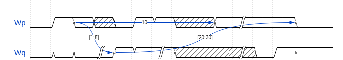
Figure 3: Timing diagram $T$ and its WaveDrom rendering.

Let $T=\langle\mathcal{W},\Sigma,C,\Theta\rangle$, $\mathcal{W}=\{W_{p}\in\textsf{Wf~{}}\ |\ p\in\Sigma\}$, be a timing diagram. Let $\nu:\Theta\to[b,e]$ be a nominal valuation. Let $\sigma:[0,n]\to 2^{\Sigma}$ be a word over $\Sigma$ and for all $p\in\Sigma$ let $\sigma_{p}:[0,n]\to\{0,1\}$ given by $\sigma_{p}(i)=1$ iff $p\in\sigma(i)$. Then the satisfaction relation $\sigma_{p}$ over a waveform $W$ under the valuation $\nu$ is defined as follows.

$$\begin{array}[]{rcl}\sigma_{p},[b,e]\models_{\nu}\textsf{0}&\mbox{iff}&e=b+1\mbox{ and }\sigma_{p}(b)=0,\\ \sigma_{p},[b,e]\models_{\nu}\textsf{1}&\mbox{iff}&e=b+1\mbox{ and }\sigma_{p}(b)=1,\\ \sigma_{p},[b,e]\models_{\nu}\lambda&\mbox{iff}&e=b+1\mbox{ and }\lambda\in\{\textsf{2},\textsf{x}\},\\ \sigma_{p},[b,e]\models_{\nu}\textsf{0}|&\mbox{iff}&\forall b\leq i<e:\sigma_{p}(i)=0,\\ \sigma_{p},[b,e]\models_{\nu}\textsf{1}|&\mbox{iff}&\forall b\leq i<e:\sigma_{p}(i)=1,\\ \sigma_{p},[b,e]\models_{\nu}\textsf{2}|&\mbox{iff}&\forall b\leq i<e:\sigma_{p}(i)\in\{0,1\},\\ \sigma_{p},[b,e]\models_{\nu}\textsf{x}|&\mbox{iff}&\forall b\leq i<e:\sigma_{p}(i)=1\mbox{ or }\forall b\leq i<e:\sigma_{p}(i)=0,\\ \sigma_{p},[b,e]\models_{\nu}u:W&\mbox{iff}&\nu(u)=b\mbox{ and }\sigma_{p},[b,e]\models_{\nu}W,\\ \sigma_{p},[b,e]\models_{\nu}VW&\mbox{iff}&\exists b\leq i<e:\sigma_{p},[b,i]\models_{\nu_{1}}V\mbox{ and }\sigma_{p},[i,e]\models_{\nu_{2}}W,\\ &&\mbox{ and }\nu_{1}||\nu\mbox{ and }\nu_{2}||\nu.\\ \end{array}$$

We say $\nu\models C$ iff $\forall(a,b,\langle l,r\rangle)\in C:\nu(b)-\nu(a)\in\langle l,r\rangle$. We define $\sigma,[b,e]\models_{\nu}\langle\mathcal{W},\Sigma,C,\Theta\rangle$ iff $\forall p\in\Sigma:\sigma_{p},[b,e]\models_{\nu}W_{p}$ and $\nu\models C$.

3.1 Waveform to SeCeNL translation

We translate a waveform $W_{p}$ to SeCeNL as follows: every 0 occurring in $P$ is translated to {{$\neg$ P}}, 1 to {{P}}, 2 and x to slen=1, 0$|$ to pt$\vee$[$\neg$ P], 1$|$ to pt$\vee$[P], 2$|$ to true, and x$|$ to pt$\vee$[P]$\vee$[$\neg$ P]. A nominal $u$ that is appearing in $W_{p}$ is translated to <u>. For instance, the waveform $W_{p}$=01a:2x011xb:x2$|$220c:00 in $T$ of Fig. 3 will be translated to SeCeNL formula as below.

({{$\neg$ P}}^{{P}}^<a>^(slen=1)^(slen=1)^{{$\neg$ P}}^{{P}}^{{P}}^(slen=1)^<b>^
				(slen=1)^true^(slen=1)^(slen=1) ^{{$\neg$ P}}^<c>^{{$\neg$ P}}^{{$\neg$ P}}).

We denote the translated SeCeNL formula by $\xi(T,W_{p})$. Similarly we can translate $W_{q}$ to get the formula $\xi(T,W_{q})$. The timing constraints in $C$ is roughly translated to the SeCeNL formula $\xi(T,C)$ as follows.

((true^<a>^((slen$\geq$ 1) $\wedge$ (slen$\leq$ 8))^<d>^true) $\wedge$

(true^<d>^((slen$\geq$ 20) $\wedge$ (slen$\leq$ 30))^<c>^true) $\wedge$

(true^<a>^(slen=10)^<b>^true)).

We define $\xi(T)=\xi(T,W_{p})\wedge\xi(T,W_{q})\wedge\xi(T,C)$. For a timing diagram $T=\langle\mathcal{W},\Sigma,C,\Theta\rangle$, $\mathcal{W}=\{W_{p}\ |\ p\in\Sigma\}$ we define $\xi(T)=\bigwedge_{p\in\Sigma}\xi(T,W_{p})\bigwedge\wedge\xi(T,C)$.

Theorem 3.1

Let $T$ be a timing diagram. Then, for all $\sigma\in\Sigma^{*}$, for all $[b,e]\in Intv(\sigma)$ and for all nominal valuation $\nu$ over $[b,e]$, $\sigma,[b,e]\models_{\nu}T$ iff $\sigma,[b,e]\models_{\nu}\xi(T):\Theta$. Also, the translation $\xi(T):\Theta$ is linear in the size of $T$.

Proof

Proof is not difficult and is by induction on the length of the waveform.

Due above theorem we can now use timing diagrams in place of nominated formulas with liveness operators. We call such timing diagrams live timing diagrams. For an example of a live timing diagram see Fig. 2.

3.2 Comparision with other temporal logics

In previous section, Lemma 3.1 showed that timing diagrams can be translated to equivalent SeCeNL formulas with only linear blowup in size. In this section we compare our logic SeCeNL with other relevent logics in the literature viz, LTL, discrete time MTL, and PSL-Sugar. Of these, PSL-Sugar is the most expressive and discrete time MTL and LTL are its syntactic subset. We show by examples that SeCeNL formulae are more succint (smaller in size) than PSL-Sugar and we believe that they capture the diagrams more directly. Appendix 0.A gives several more examples which could not be included due to lack of space.

Example (Ordered Stack)

Let us now consider the timing diagram in Fig. 4 adapted from [CF05]. Rise and fall of successive signals follow a stack discipline.

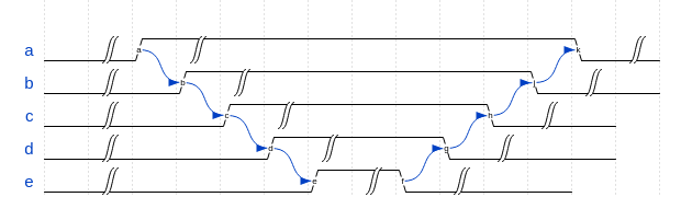
Figure 4: Example 1.

The language described by it is given by the SeCeNL formula:

$$\small\begin{array}[]{l}([\neg a]\ \textrm{\textasciicircum}\textless ua\textgreater\ \textrm{\textasciicircum}\ [a]\ \textrm{\textasciicircum}\ \textless va\textgreater\ \textrm{\textasciicircum}\ [\neg a])\ \wedge\ ([\neg b]\ \textrm{\textasciicircum}\textless ub\textgreater\ \textrm{\textasciicircum}\ [b]\ \textrm{\textasciicircum}\ \textless vb\textgreater\ \textrm{\textasciicircum}\ [\neg b])\ \wedge\\ ([\neg c]\ \textrm{\textasciicircum}\textless uc\textgreater\ \textrm{\textasciicircum}\ [c]\ \textrm{\textasciicircum}\ \textless vc\textgreater\ \textrm{\textasciicircum}\ [\neg c])\ \wedge\ ([\neg d]\ \textrm{\textasciicircum}\textless ud\textgreater\ \textrm{\textasciicircum}\ [d]\ \textrm{\textasciicircum}\ \textless vd\textgreater\ \textrm{\textasciicircum}\ [\neg d])\ \wedge\\ ([\neg e]\ \textrm{\textasciicircum}\textless ue\textgreater\ \textrm{\textasciicircum}\ [e]\ \textrm{\textasciicircum}\ \textless ve\textgreater\ \textrm{\textasciicircum}\ [\neg e])\ \wedge\ (ext~{}\ \textrm{\textasciicircum}\ \textless ua\textgreater\ \textrm{\textasciicircum}\ ext~{}\ \textrm{\textasciicircum}\ \textless ub\textgreater\ \textrm{\textasciicircum}\ ext~{})\ \wedge\\ (ext~{}\ \textrm{\textasciicircum}\ \textless ub\textgreater\ \textrm{\textasciicircum}\ ext~{}\ \textrm{\textasciicircum}\ \textless uc\textgreater\ \textrm{\textasciicircum}\ ext~{})\ \wedge\ (ext~{}\ \textrm{\textasciicircum}\ \textless uc\textgreater\ \textrm{\textasciicircum}\ ext~{}\ \textrm{\textasciicircum}\ \textless ud\textgreater\ \textrm{\textasciicircum}\ ext~{})\ \wedge\\ (ext~{}\ \textrm{\textasciicircum}\ \textless ud\textgreater\ \textrm{\textasciicircum}\ ext~{}\ \textrm{\textasciicircum}\ \textless ue\textgreater\ \textrm{\textasciicircum}\ ext~{})\ \wedge\ (ext~{}\ \textrm{\textasciicircum}\ \textless va\textgreater\ \textrm{\textasciicircum}\ ext~{}\ \textrm{\textasciicircum}\ \textless vb\textgreater\ \textrm{\textasciicircum}\ ext~{})\ \wedge\\ (ext~{}\ \textrm{\textasciicircum}\ \textless vb\textgreater\ \textrm{\textasciicircum}\ ext~{}\ \textrm{\textasciicircum}\ \textless vc\textgreater\ \textrm{\textasciicircum}\ ext~{})\ \wedge\ (ext~{}\ \textrm{\textasciicircum}\ \textless vc\textgreater\ \textrm{\textasciicircum}\ ext~{}\ \textrm{\textasciicircum}\ \textless vd\textgreater\ \textrm{\textasciicircum}\ ext~{})\ \wedge\\ (ext~{}\ \textrm{\textasciicircum}\ \textless vd\textgreater\ \textrm{\textasciicircum}\ ext~{}\ \textrm{\textasciicircum}\ \textless ve\textgreater\ \textrm{\textasciicircum}\ ext~{}).\end{array}$$

Note that first five conjuncts exactly correspond to the five waveforms. The last constraint enforces the ordering constraints between waveforms. In general, if $n$ signals are stacked, its SeCeNL specification has size $O(n)$.

An equivalent MTL (or LTL) formula is given by:

$$\begin{array}[]{l}[\neg a\ \wedge\ \neg b\ \wedge\ \neg c\ \wedge\ \neg d\ \wedge\ \neg e]\ \textbf{UU}\ [a\ \wedge\ \neg b\ \wedge\ \neg c\ \wedge\ \neg d\ \wedge\ \neg e]\ \textbf{UU}\\ \hskip 14.22636pt[a\ \wedge\ b\ \wedge\ \neg c\ \wedge\ \neg d\ \wedge\ \neg e]\ \textbf{UU}\ [a\ \wedge\ b\ \wedge\ c\ \wedge\ \neg d\ \wedge\ \neg e]\ \textbf{UU}\\ \hskip 14.22636pt[a\ \wedge\ b\ \wedge\ c\ \wedge\ d\ \wedge\ \neg e]\ \textbf{UU}\ [a\ \wedge\ b\ \wedge\ c\ \wedge\ d\ \wedge\ e]\ \textbf{UU}\\ \hskip 14.22636pt[a\ \wedge\ b\ \wedge\ c\ \wedge\ d\ \wedge\ \neg e]\ \textbf{UU}\ [a\ \wedge\ b\ \wedge\ c\ \wedge\ \neg d\ \wedge\ \neg e]\ \textbf{UU}\\ \hskip 14.22636pt[a\ \wedge\ b\ \wedge\ \neg c\ \wedge\ \neg d\ \wedge\ \neg e]\ \textbf{UU}\ [a\ \wedge\ \neg b\ \wedge\ \neg c\ \wedge\ \neg d\ \wedge\ \neg e]\ \textbf{UU}\\ \hskip 14.22636pt[\neg a\ \wedge\ \neg b\ \wedge\ \neg c\ \wedge\ \neg d\ \wedge\ \neg e]\end{array}$$

where $a\ \textbf{UU}\ b$ is the derived modality $a\ \wedge\ \textbf{X}(a\textbf{U}b)$. For a stack of $n$ signals, the size of the MTL formula is $O(n^{2})$.

Above formula is also a PSL-Sugar formula. We attempt to specify the pattern as a PSL-Sugar regular expression as follows:

$$\begin{array}[]{l}((\neg a\ \wedge\ \neg b\ \wedge\ \neg c\ \wedge\ \neg d\ \wedge\ \neg e;)[+];~{}(a\ \wedge\ \neg b\ \wedge\ \neg c\ \wedge\ \neg d\ \wedge\ \neg e;)[+];\\ \hskip 14.22636pt(a\ \wedge\ b\ \wedge\ \neg c\ \wedge\ \neg d\ \wedge\ \neg e;)[+];~{}(a\ \wedge\ b\ \wedge\ c\ \wedge\ \neg d\ \wedge\ \neg e;)[+];\\ \hskip 14.22636pt(a\ \wedge\ b\ \wedge\ c\ \wedge\ d\ \wedge\ \neg e;)[+];~{}(a\ \wedge\ b\ \wedge\ c\ \wedge\ d\ \wedge\ e;)[+];\\ \hskip 14.22636pt(a\ \wedge\ b\ \wedge\ c\ \wedge\ d\ \wedge\ \neg e;)[+];~{}(a\ \wedge\ b\ \wedge\ c\ \wedge\ \neg d\ \wedge\ \neg e;)[+];\\ \hskip 14.22636pt(a\ \wedge\ b\ \wedge\ \neg c\ \wedge\ \neg d\ \wedge\ \neg e;)[+];~{}(a\ \wedge\ \neg b\ \wedge\ \neg c\ \wedge\ \neg d\ \wedge\ \neg e;)[+];\\ \hskip 14.22636pt(\neg a\ \wedge\ \neg b\ \wedge\ \neg c\ \wedge\ \neg d\ \wedge\ \neg e;)[+]\end{array}$$

For a stack of $n$ signals, the size of the PSL-Sugar SERE expression is $O(n^{2})$. We believe that there is no formula of size $O(n)$ in PSL-Sugar which can express the above property. Compare this with size $O(n)$ formula of SeCeNL.

Example (Unordered Stack)

In ordered stack signal $a$ turns on first and turns off last followed by signals $b,c,d,e$ in that order. We consider a variation of the ordered stack example above where signals turn on and off in first-on-last-off order but there is no restriction on which signal becomes high first. This can be compactly specified in SeCeNL as follows.

$$\small\begin{array}[]{l}([\neg a]\ \textrm{\textasciicircum}\textless ua\textgreater\ \textrm{\textasciicircum}\ [a]\ \textrm{\textasciicircum}\ \textless va\textgreater\ \textrm{\textasciicircum}\ [\neg a])\ \wedge\ ([\neg b]\ \textrm{\textasciicircum}\textless ub\textgreater\ \textrm{\textasciicircum}\ [b]\ \textrm{\textasciicircum}\ \textless vb\textgreater\ \textrm{\textasciicircum}\ [\neg b])\ \wedge\\ ([\neg c]\ \textrm{\textasciicircum}\textless uc\textgreater\ \textrm{\textasciicircum}\ [c]\ \textrm{\textasciicircum}\ \textless vc\textgreater\ \textrm{\textasciicircum}\ [\neg c])\ \wedge\ ([\neg d]\ \textrm{\textasciicircum}\textless ud\textgreater\ \textrm{\textasciicircum}\ [d]\ \textrm{\textasciicircum}\ \textless vd\textgreater\ \textrm{\textasciicircum}\ [\neg d])\ \wedge\\ ([\neg e]\ \textrm{\textasciicircum}\textless ue\textgreater\ \textrm{\textasciicircum}\ [e]\ \textrm{\textasciicircum}\ \textless ve\textgreater\ \textrm{\textasciicircum}\ [\neg e])\ \wedge\ (ext~{}\ \textrm{\textasciicircum}\ \textless u1\textgreater\ \textrm{\textasciicircum}\ ext~{}\ \textrm{\textasciicircum}\ \textless u2\textgreater\ \textrm{\textasciicircum}\ ext~{})\ \wedge\\ (ext~{}\ \textrm{\textasciicircum}\ \textless u2\textgreater\ \textrm{\textasciicircum}\ ext~{}\ \textrm{\textasciicircum}\ \textless u3\textgreater\ \textrm{\textasciicircum}\ ext~{})\ \wedge\ (ext~{}\ \textrm{\textasciicircum}\ \textless u3\textgreater\ \textrm{\textasciicircum}\ ext~{}\ \textrm{\textasciicircum}\ \textless u4\textgreater\ \textrm{\textasciicircum}\ ext~{})\ \wedge\\ (ext~{}\ \textrm{\textasciicircum}\ \textless u4\textgreater\ \textrm{\textasciicircum}\ ext~{}\ \textrm{\textasciicircum}\ \textless u5\textgreater\ \textrm{\textasciicircum}\ ext~{})\ \wedge\ (ext~{}\ \textrm{\textasciicircum}\ \textless v5\textgreater\ \textrm{\textasciicircum}\ ext~{}\ \textrm{\textasciicircum}\ \textless v4\textgreater\ \textrm{\textasciicircum}\ ext~{})\ \wedge\\ (ext~{}\ \textrm{\textasciicircum}\ \textless v4\textgreater\ \textrm{\textasciicircum}\ ext~{}\ \textrm{\textasciicircum}\ \textless v3\textgreater\ \textrm{\textasciicircum}\ ext~{})\ \wedge\ (ext~{}\ \textrm{\textasciicircum}\ \textless v3\textgreater\ \textrm{\textasciicircum}\ ext~{}\ \textrm{\textasciicircum}\ \textless v2\textgreater\ \textrm{\textasciicircum}\ ext~{})\ \wedge\\ (ext~{}\ \textrm{\textasciicircum}\ \textless v2\textgreater\ \textrm{\textasciicircum}\ ext~{}\ \textrm{\textasciicircum}\ \textless v1\textgreater\ \textrm{\textasciicircum}\ ext~{})\ \wedge\\ Bijection(ua,ub,uc,ud,ue,va,vb,vc,vd,ve,u1,u2,u3,u4,u5,v1,v2,v3,v4,v5)\end{array}$$

where formula $Bijection$ below states that there is one to one correspondence between positions marked by $ua,ub,uc,ud,ue,va,vb,vc,vd,de$ and positions marked by $u1,u2,u3,u4,u5,v1,v2,v3,v4,v5$. Moreover, it states that if $u_{a}$ maps to say $u_{3}$ than $v_{a}$ must map to $v_{3}$ and so on.

$$\begin{array}[]{l}[[(u1\vee u2\vee u3\vee u4\vee u5)\Leftrightarrow(ua\vee ub\vee uc\vee ud\vee ue)]]~{}\land~{}[[\bigwedge_{1\leq i,j\leq 5,i\not=j}\neg(u_{i}\land u_{j})]]\\ \mbox{}[[(v1\vee v2\vee v3\vee v4\vee v5)\Leftrightarrow(va\vee vb\vee vc\vee vd\vee ve)]]~{}\land~{}[[\bigwedge_{1\leq i,j\leq 5,i\not=j}\neg(v_{i}\&v_{j})]]\\ \mbox{}\bigwedge_{1\leq i\leq 5,j\in a,b,c,d,e}~{}(true\ \textrm{\textasciicircum}\ \textless u_{i}\land u_{j}\textgreater\ \textrm{\textasciicircum}\ true\Leftrightarrow\ true\ \textrm{\textasciicircum}\ \textless v_{i}\land v_{j}\textgreater\ \textrm{\textasciicircum}\ true)\end{array}$$

Note that, in general, if $n$ signals are stacked, then the above SeCeNL specification has size $O(n^{2})$.

Now we discuss encoding of unordered stack in PSL-Sugar. In absence of nominals, it is difficult to state the above behaviour succinctly in logics PSL-Sugar even using its SERE regular expressions. Each order of occurrence of signals has to be enumerated as a disjunction where each disjunct is as in the example ordered stack (where the order was $a,b,c,d,e$). As there are $n!$ orders possible between $n$ signals, the size of the PSL-Sugar formula is also $O(n!)$. We believe that there is no polynomially sized formula in PSL-Sugar encoding this property. This shows that SeCeNL is exponentially more succint as compared to PSL-Sugar.

In general, presence of nominals distinguishes SeCeNL from logics like PSL-Sugar. In formalizing behaviour of hardware circuits it has been proposed that regular expressions are not enough and operators such as pipelining have been introduced [CF05]. These are a form of synchronization and they can be easily expressed using nominals too.

4 Case study: Minepump Specification

We first specify some useful generic timing diagram properties which would used for requirement specification in this (and many other) case studies.

• $\textbf{lags}(P,Q,n)$: it is defined by Fig. 8. It specifies that in any observation interval if $P$ holds continuously for $n+1$ cycles and persists then $Q$ holds from $(n+1)^{th}$ cycle onwards and persists till $P$ persists.

• $\textbf{tracks}(P,Q,n)$: defined Fig. 8. In any observation interval if $P$ becomes true then $Q$ sustains as long as $P$ sustains or upto $n$ cycles whichever is shorter.

• $\textbf{sep}(P,n)$: Fig. 8 defines this property. Any interval which begins with a falling edge of $P$ and ends with a rising edge of $P$ then the length of the interval should be at least $n$ cycles.

• $\textbf{ubound}(P,n)$: Fig. 8 defines the property. In any observation interval $P$ can be continuously true for at most $n$ cycles.

Note that we have presented these formulae diagrammatically. The textual version of these live timing diagrams can be found in Appendix 0.C.

Figure 5: $\textbf{lags}(P,Q,n)$.

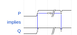
Figure 6: $\textbf{tracks}(P,Q,n)$.

Figure 7: $\textbf{sep}(P,n)$.

Figure 8: $\textbf{ubound}(P,n)$.

We now state the minepump problem. Imagine a minepump which keeps the water level in a mine under control for the safety of miners. The pump is driven by a controller which can switch it on and off. Mines are prone to methane leakage trapped underground which is highly flammable. So as a safety measure if a methane leakage is detected the controller is not allowed to switch on the pump under no circumstances.

The controller has two input sensors - HH2O which becomes 1 when water level is high, and HCH4 which is 1 when there is a methane leakage; and can generate two output signals - ALARM which is set to 1 to sound/persist the alarm, and PUMPON which is set to 1 to switch on the pump. The objective of the controller is to safely operate the pump and the alarm in such a way that the water level is never dangerous, indicated by the indicator variable DH2O, whenever certain assumptions hold. We have the following assumptions on the mine and the pump.

• Sensor reliability assumption: $\mbox{{pref}}([[DH2O\Rightarrow HH2O]])~{}$. If HH2O is false then so is DH2O.

• Water seepage assumptions: $\textbf{tracks}(HH2O,DH2O,\kappa_{1})$. The minimum no. of cycles for water level to become dangerous once it becomes high is $\kappa_{1}$.

• Pump capacity assumption: $\textbf{lags}(PUMPON,\neg HH2O,\kappa_{2})$. If pump is switched on for at least $\kappa_{2}+1$ cycles then water level will not be high after $\kappa_{2}$ cycles.

• Methane release assumptions: $\textbf{sep}(HCH4,\kappa_{3})$ and $\textbf{ubound}(HCH4,\kappa_{4})$. The minimum separation between the two leaks of methane is $\kappa_{3}$ cycles and the methane leak cannot persist for more than $\kappa_{4}$ cycles.

• Initial condition assumption: $\textbf{init}(\textless\neg HH2O\textgreater\wedge\textless\neg HCH4\textgreater,slen=0)$. Initially neither the water level is high nor there is a methane leakage.

Let the conjunction of these SeCeNL formulas be denoted as $MINEASSUME$.

The commitments are:

• Alarm control: $\textbf{lags}(HH2O,ALARM,\kappa_{5})$ and $\textbf{lags}(HCH4,ALARM,\kappa_{6})$ and $\textbf{lags}(\neg HH2O\ \wedge\ \neg HCH4,\neg ALARM,\kappa_{7})$. If the water level is dangerous then alarm will be high after $\kappa_{5}$ cycles and if there is a methane leakage then alarm will be high after $\kappa_{6}$ cycles. If neither the water level is dangerous nor there is a methane leakage then alarm should be off after $\kappa_{7}$ cycle.

• Safety condition: $\mbox{{pref}}([[\neg DH2O\ \wedge\ (HCH4$$\Rightarrow$$\neg PUMPON)]])~{}$. The water level should never become dangerous and whenever there is a methane leakage pump should be off.

Let the conjunction of these commitments be denoted as $MINECOMMIT$. Then the requirement over the minepump controller is given by the formula $MINEASSUME\Rightarrow MINECOMMIT$. A textual version of this full minepump specification, which can be input to our tools is given in Appendix 0.C. Note that the require consists of a mixture of timing diagram constraints (such as pump capacity assumption above) as well as SeCeNL formulas (such as Safety condition above).

We can automatically synthesize a controller for the values say $\kappa_{1}=10$, $\kappa_{2}=2$, $\kappa_{3}=14$, $\kappa_{4}=2$, and $\kappa_{5}=\kappa_{6}=\kappa_{7}=1$. The tool outputs a SCADE/SMV controller meeting the specification. A snapshot of SCADE code for the controller synthesized by DCSynthG for minepump can be found in Appendix 0.D. If the specification is not realizable we output an explanation.

A second case study of synchronous bus arbiter specification can be found in Appendix. 0.E. We can automatically synthesize a property monitor for such requirement and use it to model check a given arbiter design; or we can directly synthesize a controller meeting the requirement. The appendix gives results of both these experiments.

Appendix 0.A Examples of Comparision with other logics

Example 1 (Ordering with timing)

Consider the timing diagram in Fig. 9 which says that $a$ holds invariantly in the interval $[0,i]$ where $i\geq 1$, $b$ holds invariantly in the interval $[i,j]$, $j\geq i+1$, and $c$ holds at $j$ and $j\leq n$.

Figure 9: Example 1.

• The language described by the above timing diagram is given by the SeCeNL formula $([a\wedge\neg b]\ \textrm{\textasciicircum}\ [b\wedge\neg a\wedge\neg c]\ \textrm{\textasciicircum}\ \textless c\textgreater)\ \wedge\ (\textsf{slen}\leq n)$ which is of size $O(\log(n))$. It is assumed that all timing constants such as $n$ are encoded in binary and hence they contribute size $\log(n)$.

• An equivalent MTL formula is $\bigvee_{i=1}^{i=n-1}(a\wedge\neg b\textbf{U}[i,i](b\wedge\neg a\textbf{U}[1,n-i]\ c))$ whose size is $O(n\log(n))$.

• Equivalent LTL formula is $\bigvee_{i=1}^{i=n-1}\bigvee_{j=1}^{j=n-i}(a\ \textbf{U}\textbf{X}^{i}(b\ \textbf{U}\textbf{X}^{j}\ c))$ where $\textbf{X}^{k}=\underbrace{\textbf{X}\cdot\ldots\cdot\textbf{X}}_{k\mbox{ times}}$, whose size is $O(n^{2})$.

• Equivalent PSL-Sugar formula is $(a\wedge\neg b[+];~{}b\wedge\neg a\wedge\neg c[+];~{}c)\wedge((a|b)[<n];c)$ with size $O(\log(n))$.

We also give examples of complex dependancy constraints. Consider the timing diagram in Fig. 10. In this diagram, $ua$ occurs before $ub$ and $uc$, and $uc$ occurs before $ud$ and $ue$. The point $vc$ occurs after $vd$ and $ve$, and $va$ occurs after $vb$ and $vb$.

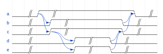
Figure 10: Example 3.

The behaviour is described straightforwardly by the SeCeNL formula:

$$\small\begin{array}[]{l}([\neg a]\ \textrm{\textasciicircum}\textless ua\textgreater\textrm{\textasciicircum}\ [a]\ \textrm{\textasciicircum}\textless va\textgreater\textrm{\textasciicircum}\ [\neg a])\ \wedge\ ([\neg b]\ \textrm{\textasciicircum}\textless ub\textgreater\ \textrm{\textasciicircum}\ [b]\ \textrm{\textasciicircum}\textless vb\textgreater\textrm{\textasciicircum}[\neg b])\ \wedge\\ ([\neg c]\ \textrm{\textasciicircum}\ \textless uc\textgreater\ \textrm{\textasciicircum}\ [c]\ \textrm{\textasciicircum}\ \textless vc\textgreater\ \textrm{\textasciicircum}\ [\neg c])\ \wedge\ ([\neg d]\ \textrm{\textasciicircum}\ \textless ud\textgreater\ \textrm{\textasciicircum}\ [d]\ \textrm{\textasciicircum}\textless vd\textgreater\ \textrm{\textasciicircum}\ [\neg d])\ \wedge\\ ([\neg e]\ \textrm{\textasciicircum}\ \textless ue\textgreater\ \textrm{\textasciicircum}\ [e]\ \textrm{\textasciicircum}\ \textless ve\textgreater\ \textrm{\textasciicircum}\ [\neg e])\ \wedge\ (ext~{}\ \textrm{\textasciicircum}\ \textless ua\textgreater\ \textrm{\textasciicircum}\ ext\ \textrm{\textasciicircum}\ \textless ub\textgreater\ \textrm{\textasciicircum}\ true)\ \wedge\\ (ext~{}\ \textrm{\textasciicircum}\ \textless ua\textgreater\ \textrm{\textasciicircum}\ ext\ \textrm{\textasciicircum}\ \textless uc\textgreater\ \textrm{\textasciicircum}\ true)\ \wedge\ (ext~{}\ \textrm{\textasciicircum}\ \textless uc\textgreater\ \textrm{\textasciicircum}\ ext\ \textrm{\textasciicircum}\ \textless ud\textgreater\ \textrm{\textasciicircum}\ true)\ \wedge\\ (ext~{}\ \textrm{\textasciicircum}\ \textless uc\textgreater\ \textrm{\textasciicircum}\ ext\ \textrm{\textasciicircum}\ \textless ue\textgreater\ \textrm{\textasciicircum}\ true)\ \wedge\ (ext~{}\ \textrm{\textasciicircum}\ \textless ve\textgreater\ \textrm{\textasciicircum}\ ext\ \textrm{\textasciicircum}\ \textless vc\textgreater\ \textrm{\textasciicircum}\ true)\ \wedge\\ (ext~{}\ \textrm{\textasciicircum}\ \textless vd\textgreater\ \textrm{\textasciicircum}\ ext\ \textrm{\textasciicircum}\ \textless vc\textgreater\ \textrm{\textasciicircum}\ true)\ \wedge\ (ext~{}\ \textrm{\textasciicircum}\ \textless vc\textgreater\ \textrm{\textasciicircum}\ ext\ \textrm{\textasciicircum}\ \textless va\textgreater\ \textrm{\textasciicircum}\ true)\ \wedge\\ (ext~{}\ \textrm{\textasciicircum}\ \textless vb\textgreater\ \textrm{\textasciicircum}\ ext\ \textrm{\textasciicircum}\ \textless va\textgreater\ \textrm{\textasciicircum}\ true).\end{array}$$

This formula is linear in the size of the timing diagram. Unfortunately, specifying these dependancies in PSL-Sugar is complex and formula size blows up at least quadratically.

Appendix 0.B Implementation

We propose a textual framework with a well defined syntax and semantics for requirement specification (of the form assumptions $\Rightarrow$ commitments). Our framework is heterogeneous in the sense that it supports both SeCeNL formulas and timing diagrams with nominals for system specification. It can also handle all of our limited liveness operators. (see Appendix. 0.C for the code for minepump in our framework).

We have also developed a Python based translator which takes requirements in our textual format as input and produces property monitors as well as controllers as output. Fig. 11 gives a broad picture of the current status of our tool chain.

Figure 11: Our tool chain.

Appendix 0.C Minepump Code

The example code for minepump is written using textual syntax for QDDC which can be found in [Pan00, Pan01].

#lhrs ”minepump”
interface
{

input HH2O, HCH4;

output ALARM monitor x, PUMPON monitor x;

constant delta = 1, w = 10, epsilon=2 , zeta=14, kappa=2;

auxvar DH2O;

softreq (!YHCH4)$||$(!PUMPON);
}
#implies lag(P, Q, n)
{

td lagspeclet1(P, n)

{

P:<u>1$|$<v>1$|$;

@sync:(u, v, n);

}

td lagspeclet2(Q)

{

Q: 2$|$<v>1$|$;

}
}
#implies tracks(P, Q, n)
{

td tracksspeclet1(P, n)

{

P: 0<u>1$|$<v>1$|$;

@sync: (u,v,[n,));

}

td tracksspeclet2(Q)

Q: 2<u>1$|$<v>0$|$;
}
#implies tracks2(P, Q, n)

td tracks2speclet1(P, n)

{

P: 0<u>1$|$<v>0$|$;

@sync: (u,v,[,n]);

}

td tracks2speclet2(Q)

Q:2<u>0$|$<v>2$|$;
}
#implies sep(P, n)
{

td sepspeclet1(P)

P: 1<u>0$|$<v>1;

td sepspeclet2(n)

{

@null: 2<u>2$|$<v>2;

@sync: (u, v, (n,]);

}
}
#implies ubound(P, n)
{

td boundspeclet1(P)

P: <c>1$|$<d>1;

td boundspeclet2(n)

{

@null: <c>2$|$<d>2;

@sync: (c, d, [,n));

}
}
dc safe(DH2O) {

pt $||$ [!DH2O && ((HCH4$||$!HH2O) =>!PUMPON)];
}
main()
{

assume (<!HH2O> ^ true);

assume (pt $||$ [DH2O =>HH2O]);

assume tracks(HH2O, !DH2O, w);

assume tracks2 (HH2O, DH2O, w);

assume lag(PUMPON, !HH2O, epsilon);

assume sep(HCH4, zeta);

assume ubound(HCH4, kappa);

req (<!ALARM> ^ true);

req lag(HH2O, ALARM, delta);

req lag(HCH4, ALARM, delta);

req lag(!HCH4 && !HH2O, !ALARM, delta);

req safe(DH2O);
}

Appendix 0.D Synthesized controller for minepump

A snapshot of a controller synthesized from the minepump requirement in §4. The controller had approximately 140 states and it took less than a second for synthesis.

$\begin{array}[]{l}\mathrm{\textsf{node minepump ( HH2O, HCH4:bool) returns ( ALARM, PUMPON:bool)}}\\ \mathrm{\textsf{var cstate: int; }}\\ \mathrm{\textsf{let }}\\ \mathrm{\textsf{\qquad ALARM, PUMPON, cstate = }}\\ \mathrm{\textsf{\qquad( if true and not HH2O and not HCH4 then ( false, false, 2) }}\\ \mathrm{\textsf{\qquad else if true and not HH2O and HCH4 then ( false, false, 4) }}\\ \mathrm{\textsf{\qquad else if true and HH2O and not HCH4 then ( false, false, 4) }}\\ \mathrm{\textsf{\qquad else if true and HH2O and HCH4 then ( false, false, 4) }}\\ \mathrm{\textsf{\qquad else ( dontCare, dontCare, 1)) $\Rightarrow$}}\\ \mathrm{\textsf{\qquad if pre cstate = 1 and not HH2O and not HCH4 then ( false, false, 2) }}\\ \mathrm{\textsf{\qquad else if pre cstate = 1 and not HH2O and HCH4 then ( false, false, 4) }}\\ \mathrm{\textsf{\qquad else if pre cstate = 1 and HH2O and not HCH4 then ( false, false, 4) }}\\ \mathrm{\textsf{\qquad else if pre cstate = 1 and HH2O and HCH4 then ( false, false, 4) }}\\ \mathrm{\textsf{\qquad else if pre cstate = 2 and not HH2O and not HCH4 then ( false, false, 2) }}\\ \mathrm{\textsf{\qquad else if pre cstate = 2 and not HH2O and HCH4 then ( false, false, 7) }}\\ \mathrm{\textsf{\qquad else if pre cstate = 2 and HH2O and not HCH4 then ( false, false, 9) }}\\ \mathrm{\textsf{\qquad else if pre cstate = 2 and HH2O and HCH4 then ( false, false, 11) }}\\ \mathrm{\textsf{\qquad else if pre cstate = 4 and not HH2O and not HCH4 then ( false, false, 4) }}\\ \mathrm{\textsf{\qquad else if pre cstate = 4 and not HH2O and HCH4 then ( false, false, 4) }}\\ \mathrm{\textsf{\qquad..............................}}\\ \mathrm{\textsf{\qquad..............................}}\\ \mathrm{\textsf{\qquad else if pre cstate = 309 and HH2O and not HCH4 then ( false, true, 4) }}\\ \mathrm{\textsf{\qquad else if pre cstate = 309 and HH2O and HCH4 then ( false, true, 4) }}\\ \mathrm{\textsf{\qquad else if pre cstate = 372 and not HH2O and not HCH4 then ( false, false, 2) }}\\ \mathrm{\textsf{\qquad else if pre cstate = 372 and not HH2O and HCH4 then ( false, false, 7) }}\\ \mathrm{\textsf{\qquad else if pre cstate = 372 and HH2O and not HCH4 then ( false, true, 4) }}\\ \mathrm{\textsf{\qquad else if pre cstate = 372 and HH2O and HCH4 then ( false, true, 4) }}\\ \mathrm{\textsf{\qquad else ( dontCare, dontCare, pre cstate) ; }}\\ \mathrm{\textsf{tel }}\\ \end{array}$

Appendix 0.E Case study: 3-cell arbiter

In this section we illustrate another application of our specification format and associated tools. For this we use the standard McMillan arbiter circuit given in NuSMV examples and do the model checking against the specification below.

A synchronous 3-cell bus arbiter has 3 request lines $req1,req2$ and $req3$, and corresponding acknowledgement lines $ack1,ack2$ and $ack3$. At any time instance a subset of request lines can be high and arbiter decides which request should be granted permission to access the bus by making corresponding acknowledgement line high. The requirements for such a bus arbiter are as formulated below.

• Exclusion: $\mbox{{pref}}([[(\bigwedge_{i\neq j}\neg(ack_{i}\wedge ack_{j}))]])~{}$. At most 1 acknowledgement can be given at a time.

• No spurious acknowledgement: $\mbox{{pref}}([[(\bigwedge_{1}(ack_{i}\Rightarrow req_{i}))]])~{}$. A request should be granted access to the bus only if it has requested it.

• Response time: $\textbf{implies}([[req]]\wedge slen=n,true~{}\verb|^|\textless ack\textgreater\verb|^|true~{})$. One of the most important property of an arbiter is that it any request should be granted within $n$ cycles, i. e. if a request is continuously true for sometime then it should be heard.

• Deadtime: to specify this property we first specify lost cycle as follows: $Lost\equiv(\bigvee_{i}req_{i})\wedge(\neg(\bigvee_{i}ack_{i}))$. Then $Deadtime\equiv\textbf{anti}([[Lost]]\wedge slen>n)$. This specifies the maximum number of consecutive cycles that can be lost by the arbiter is $n$.

The requirement $ARBREQ$ is a conjunction of above formulas.

We ran the requirement through our tool chain to generate NuSMV module for the requirement monitor. This module was then instantiated synchronously with McMillan arbiter implementation in NuSMV and NuSMV model checker was called in to check the property $G(assumptions\Rightarrow commitments)$.

Model checking

: Experimental results show that the deadtime for 3-cell McMillan arbiter is 3. If we specify the deadtime as 2 cycles then a counter example is generated by NuSMV as depicted in Fig. 14. This counter examples show that even though there is an request line high in $4^{th}$, $5^{th}$ and $6^{th}$ cycle, but no acknowledgment is given by arbiter. Similarly, the response time for $1^{st}$ request is 3 cycles whereas for $2^{nd}$ and $3^{rd}$ cell it is 6 cycles. If we specify the response time of 2 and 5 cycles for $1^{st}$ and $2^{nd}$ then NuSMV generates counter examples in Fig. 14 and Fig. 14 respectively. Fig. 14 shows that the request line for cell 2 (i. e. req2) is high continuously for 5 cycles starting from $3^{rd}$ without an acknowledgement from the arbiter.

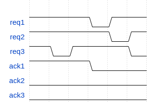
Figure 12: Counter Example Showing deadtime exceeding 2 cycles

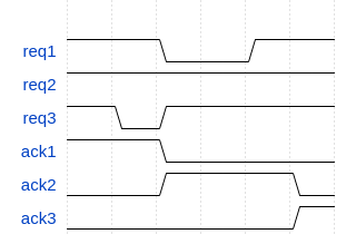
Figure 13: Counter Example showing response time of 1st cell exceeding 2 cycles

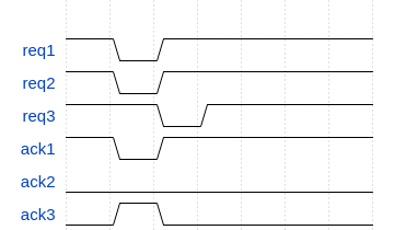
Figure 14: Counter Example showing response time of 2nd cell exceeding 5 cycles

Controller synthesis

: We have also synthesized a controller for the arbiter specification using our tool DCSynthG. We have tightened the requirements by specifying the response time as 3 cycles uniformly for all three cells and deadtime as 0 cycles, i. e. there is no lost cycle. The tool could synthesize a controller in 0.03 seconds with 17 states.

References

- [AEKN00] Nina Amla, E. Allen Emerson, Robert P. Kurshan, and Kedar S. Namjoshi. Model checking synchronous timing diagrams. In Warren A. Hunt Jr. and Steven D. Johnson, editors, Formal Methods in Computer-Aided Design, Third International Conference, FMCAD 2000, Austin, Texas, USA, November 1-3, 2000, Proceedings, volume 1954 of Lecture Notes in Computer Science, pages 283–298. Springer, 2000.
- [AH93] Rajeev Alur and Thomas A. Henzinger. Real-time logics: Complexity and expressiveness. Inf. Comput., 104(1):35–77, 1993.
- [All83] James F. Allen. Maintaining knowledge about temporal intervals. Commun. ACM, 26(11):832–843, 1983.
- [AS87] Bowen Alpern and Fred B. Schneider. Recognizing safety and liveness. Distributed Computing, 2(3):117–126, 1987.
- [BP12] Ajesh Babu and Paritosh K. Pandya. Chop expressions and discrete duration calculus. In Modern Applications of Automata Theory, pages 229–256. 2012.
- [CF05] Hana Chockler and Kathi Fisler. Temporal modalities for concisely capturing timing diagrams. In Dominique Borrione and Wolfgang J. Paul, editors, Correct Hardware Design and Verification Methods, 13th IFIP WG 10.5 Advanced Research Working Conference, CHARME 2005, Saarbrücken, Germany, October 3-6, 2005, Proceedings, volume 3725 of Lecture Notes in Computer Science, pages 176–190. Springer, 2005.
- [CP16] Aliaksei Chapyzhenka and Jonah Probell. Wavedrom: Rendering beautiful waveforms from plain text. Synopsys User Group, 2016.
- [DH01] Werner Damm and David Harel. Lscs: Breathing life into message sequence charts. Formal Methods in System Design, 19(1):45–80, 2001.
- [EF16] Cindy Eisner and Dana Fisman. Temporal logic made practical. Handbook of Model Checking. Springer (Expected 2016), http://www. cis. upenn. edu/~ fisman/documents/EF_HBMC14. pdf, 2016.
- [FdRS03] Massimo Franceschet, Maarten de Rijke, and Bernd-Holger Schlingloff. Hybrid logics on linear structures: Expressivity and complexity. In 10th International Symposium on Temporal Representation and Reasoning / 4th International Conference on Temporal Logic (TIME-ICTL 2003), 8-10 July 2003, Cairns, Queensland, Australia, pages 166–173. IEEE Computer Society, 2003.
- [Fis99] Kathi Fisler. Timing diagrams: Formalization and algorithmic verification. Journal of Logic, Language and Information, 8(3):323–361, 1999.
- [Fis07] Kathi Fisler. Two-dimensional regular expressions for compositional bus protocols. In Formal Methods in Computer-Aided Design, 7th International Conference, FMCAD 2007, Austin, Texas, USA, November 11-14, 2007, Proceedings, pages 154–157. IEEE Computer Society, 2007.
- [KP05] Yonit Kesten and Amir Pnueli. A compositional approach to CTL* verification. Theor. Comput. Sci., 331(2-3):397–428, 2005.
- [Pan00] Paritosh K. Pandya. Specifying and deciding quantified discrete-time duration calculus formulae using DCVALID. Technical report, Tata Institute of Fundamental Research, Mumbai, 2000.
- [Pan01] Paritosh K. Pandya. Model checking ctl*[dc]. In Tiziana Margaria and Wang Yi, editors, Tools and Algorithms for the Construction and Analysis of Systems, 7th International Conference, TACAS 2001 Held as Part of the Joint European Conferences on Theory and Practice of Software, ETAPS 2001 Genova, Italy, April 2-6, 2001, Proceedings, volume 2031 of Lecture Notes in Computer Science, pages 559–573. Springer, 2001.
- [Wav16] WaveDrom. Wavedrom user manual. http://wavedrom.com/tutorial.html, 2016.