First eigenvalue estimates of Dirichlet-to-Neumann operators on graphs

Abstract.

Following Escobar [Esc97] and Jammes [Jam15], we introduce two types of isoperimetric constants and give lower bound estimates for the first nontrivial eigenvalues of Dirichlet-to-Neumann operators on finite graphs with boundary respectively.

1. Introduction

Let $(M,g)$ be a compact manifold with boundary $\partial{M}$. The Dirichlet-to-Neumann operator $\Lambda:H^{\frac{1}{2}}(\partial M)\longrightarrow H^{-\frac{1}{2}}(\partial M)$ is defined as

$$\Lambda(f)=\frac{\partial u_{f}}{\partial n},$$

where $u_{f}$ is the harmonic extension of $f\in H^{\frac{1}{2}}(\partial M)$. The Dirichlet-to-Neumann operator is a first order elliptic pseudo-differential operator [Tay96, page 37] and its associated eigenvalue problem is also known as the Steklov problem, see [KKK⁺14] for a historical discussion. Since $\partial M$ is compact, the spectrum of $\Lambda$ is nonnegative, discrete and unbounded [Ban80, page95].

The Dirichlet-to-Neumann operator is closely related to the $\mathrm{Calder\acute{o}n}$ problem [Cal80] of determining the anisotropic conductivity of a body from current and voltage measurements at its boundary. This makes it useful for applications to electrical impedance tomography, which is used in medical and geophysical imaging, see [Uhl14] for a recent survey.

Eigenvalue estimates are of interest in spectral geometry. In [Che70], Cheeger discovered a close relation between the geometric quantity, the isoperimetric constant (also called the Cheeger constant), and the analytic quantity, the first nontrivial eigenvalue of the Laplace-Beltrami operator on a closed manifold. Estimate of this type is called the Cheeger estimate.

For the first nontrivial eigenvalue of the Dirichlet-to-Neumann operator, two different types of lower bound estimates, which are similar to the classical Cheeger estimate, have been obtained by Escobar and Jammes respectively in [Esc97] and [Jam15]. For convenience, we call them the Escobar-type Cheeger estimate and the Jammes-type Cheeger estimate.

The Cheeger constant introduced by Escobar [Esc97], which we call the Escobar-type Cheeger constant, is defined as

$$h_{E}(M):=\inf_{\mathrm{Area}(\Omega\cap\partial M)\leq\frac{1}{2}\mathrm{Area}(\partial M)}\frac{\mathrm{Area}(\partial\Omega\cap\mathrm{int}(M))}{\mathrm{Area}(\Omega\cap\partial M)},$$

where $\mathrm{Area}(\cdot)$ denotes the codimensional one Hausdorff measure, i.e. the Riemannian area, and $\mathrm{int}(M)$ denotes the interior of the manifold $M$. Let $\sigma_{1}$ be the first nontrivial eigenvalue of the Dirichlet-to-Neumann operator $\Lambda$, then the Escobar-type Cheeger estimate [Esc97, Theorem 10] reads as

$$\sigma_{1}\geq\frac{\left(h_{E}(M)\mu_{1}(k)-ak\right)a}{a^{2}+\mu_{1}(k)},$$

where $a>0$, $k>0$ are arbitrary positive constants, and $\mu_{1}(k)$ is the first eigenvalue of the following Robin problem

$$\left\{\begin{array}[]{ll}\Delta u+\mu_{1}(k)u=0,&\text{on\ }M,\\ \frac{\partial u}{\partial n}+ku=0,&\text{on\ }\partial M.\end{array}\right.$$

The Jammes-type Cheeger constant, which was introduced in [Jam15], is defined as

$$h_{J}(M)=\inf_{\mathrm{Vol}(\Omega)\leq\frac{1}{2}{\mathrm{Vol}(M)}}\frac{\mathrm{Area}(\partial\Omega\cap\mathrm{int}(M))}{\mathrm{Area}(\Omega\cap\partial M)},$$

where $\mathrm{Vol}(\cdot)$ denotes the Riemannian volume. The Jammes-type Cheeger estimate [Jam15, Theorem 1] is given as follows

$$\sigma_{1}\geq\frac{1}{4}h(M)h_{J}(M),$$

where $h(M)$ is the classical Cheeger constant associated to the Laplacian operator with Neumann boundary condition on $M$, which is defined as

$$h(M)=\inf_{\mathrm{Vol}(\Omega)\leq\frac{1}{2}{\mathrm{Vol}(M)}}\frac{\mathrm{Area}(\partial\Omega\cap\mathrm{int}(M))}{\mathrm{Vol}(\Omega)}.$$

The Dirichlet-to-Neumann operator is naturally defined in the discrete setting. We recall some basic definitions on graphs. Let $V$ be a countable set which serves as the set of vertices of a graph and $\mu$ be a symmetric weight function given by

$$\mu:V\times V \to[0,\infty),$$

$$(x,y) \mapsto\mu_{xy}=\mu_{yx}.$$

This induces a graph structure $G=(V,E)$ with the set of vertices $V$ and the set of edges $E$ which is defined as $\{x,y\}\in E$ if and only if $\mu_{xy}>0,$ in symbols $x\sim y.$ Note that we do allow self-loops in the graph, i.e. $x\sim x$ if $\mu_{xx}>0.$ Given $\Omega_{1},\Omega_{2}\subset V$, the set of edges between $\Omega_{1}$ and $\Omega_{2}$ is denoted by

$$E(\Omega_{1},\Omega_{2}):=\{e=\{x,y\}\in E|x\in\Omega_{1},y\in\Omega_{2}\}.$$

For any subset $\Omega\subset V$, there are two notions of boundary, i.e. the edge boundary and the vertex boundary. The edge boundary of $\Omega$, denoted by $\partial\Omega$, is defined as

$$\partial\Omega:=E(\Omega,\Omega^{c}),$$

where $\Omega^{c}:=V\setminus\Omega$. The vertex boundary of $\Omega$, denoted by $\delta\Omega$, is defined as

$$\delta\Omega:=\{x\in V\setminus\Omega|\ x\sim y\mathrm{\ for\ some\ }y\in\Omega\}.$$

Set $\overline{\Omega}:=\Omega\cup\delta\Omega$. We introduce a measure on $\overline{\Omega}$, $m:\overline{\Omega}\rightarrow(0,\infty)$, as follows

$$m_{x}=\left\{\begin{array}[]{ll}\sum_{y\in V,y\sim x}\mu_{xy},&x\in\Omega,\\ \sum_{y\in\Omega,y\sim x}\mu_{xy},&x\in\delta\Omega.\end{array}\right.$$

Accordingly, $m(A):=\sum_{x\in A}m_{x}$ denotes the measure of any subset $A\subset\overline{\Omega}$. Given any set $F,$ we denote by ${\mathbb{R}}^{F}$ the collection of all real functions defined on $F.$

For any finite subset $\Omega\subset V$, in analogy to the Riemannian case, one can define the Dirichlet-to-Neumann operator in the discrete setting to be

$$\Lambda:{\mathbb{R}}^{\delta\Omega} \to{\mathbb{R}}^{\delta\Omega},$$

$$\varphi \mapsto\Lambda\varphi:=\frac{\partial u_{\varphi}}{\partial n},$$

where $u_{\varphi}$ is the harmonic extension of $\varphi$ to $\Omega$, and $\frac{\partial}{\partial n}$ is the outward normal derivative in the discrete setting defined as in (2.1) in section 2. We call $\Lambda$ the DtN operator for short. Let $\sigma(\Lambda)$ denote the spectrum of $\Lambda$. By the definition of $\Lambda$ and Green’s formula, see Lemma 2.1, $\Lambda$ is a nonnegative self-adjoint operator, i.e. $\sigma(\Lambda)$ is a set of nonnegative real numbers. In fact, $\sigma(\Lambda)$ is contained in $[0,1]$, see Proposition 3.1.

It is well known that the eigenvalues of (normalized) Laplace operators on finite graphs without any boundary condition are contained in $[0,2]$. The multiplicity of eigenvalue 0 is equal to the number of connected components of the graph, see [BH12, Prop.1.3.7]. The largest possible eigenvalue 2 is achieved if and only if the graph is bipartite, see [Gri09, Theorem 2.3]. Similar results can be generalized to the case of DtN operators. For convenience, let $\widetilde{\Omega}$ denote the graph with vertices in $\overline{\Omega}$ and edges in $E(\Omega,\overline{\Omega})$, i.e.

(1.1) $$\widetilde{\Omega}:=(\overline{\Omega},E(\Omega,\overline{\Omega})).$$

From Proposition 3.2, we know that the multiplicity of eigenvalue 0 of $\Lambda$ is equal to the number of connected components of $\widetilde{\Omega}$. Moreover, we show that the eigenspace associated to the eigenvalue 1 which is the largest possible eigenvalue is the kernel of a linear operator $Q$ whose definition is given in (3.2) below.

Given $A\subset\overline{\Omega}$, we denote by

$$\partial_{\Omega}A:=\partial A\cap E(\Omega,\overline{\Omega})$$

the relative boundary and $A^{\vee}:=\overline{\Omega}\setminus A$ the relative complement of $A$ in $\widetilde{\Omega}$. Without loss of generality, we always assume that $\widetilde{\Omega}$ is connected.

Now we consider the first nontrivial eigenvalue estimates of DtN operators on finite graphs. We introduce two isoperimetric constants following Escobar and Jammes, which we call Escobar-type Cheeger constant and Jammes-type Cheeger constant respectively.

Definition 1.1.

The Escobar-type Cheeger constant for $\widetilde{\Omega}$ is defined as

$$h_{E}(\widetilde{\Omega}):=\inf_{m(A\cap\delta\Omega)\leq\frac{1}{2}m(\delta\Omega)}\frac{\mu(\partial_{\Omega}A)}{m(A\cap\delta\Omega)}.$$

The Jammes-type Cheeger constant for $\widetilde{\Omega}$ is defined as

$$h_{J}(\widetilde{\Omega}):=\inf_{m(A)\leq\frac{1}{2}{m(\overline{\Omega})}}\frac{\mu(\partial_{\Omega}A)}{m(A\cap\delta\Omega)}.$$

By definitions, one has $h_{J}(\widetilde{\Omega})\leq h_{E}(\widetilde{\Omega})$, see Proposition 4.1. This estimate is optimal, see Example 4.1 in the paper.

To derive the Cheeger estimates, we first show that $h_{E}(\widetilde{\Omega})$ is equal to a type of Sobolev constant. Similar results can be found in both Riemannian and discrete case, see e.g. [Li12, Cha16, Chu97].

Theorem 1.1.

Let $G$ be a finite graph and $\Omega\subset V,$ then

$$h_{E}(\widetilde{\Omega})=\inf_{f\in{\mathbb{R}}^{\overline{\Omega}}}\frac{\sum_{e=\{x,y\}\in E(\Omega,\overline{\Omega})}\mu_{xy}|f(x)-f(y)|}{\inf_{a\in{\mathbb{R}}}\sum_{x\in\delta\Omega}m_{x}|f(x)-a|}.$$

Without loss of generality, we assume that the number of vertices in $\delta\Omega$ is at least two. From now on, we denote by $\lambda_{1}(\Omega)$ the first nontrivial eigenvalue of the DtN operator $\Lambda$ on $\Omega$ in a finite graph. In the discrete setting, it’s easy to obtain an upper bound estimate as

$$\lambda_{1}(\Omega)\leq 2h_{E}(\widetilde{\Omega}),$$

see Proposition 4.2. The sharpness of this upper bound can be seen from Example 4.2. For the lower bound estimate, we obtain the Escobar-type Cheeger estimate as follows.

Theorem 1.2.

Let $G$ be a finite graph and $\Omega\subset V,$ then

(1.2) $$\lambda_{1}(\Omega)\geq\frac{\left(2h_{E}(\widetilde{\Omega})\mu_{1}(k)-a(k+\mu_{1}(k))\right)a}{a^{2}+2\mu_{1}(k)},$$

where $a>0$, $k>0$ are arbitrary positive constants, and $\mu_{1}(k)$ is the first eigenvalue of the Robin problem

$$\left\{\begin{array}[]{ll}\Delta u+\mu_{1}(k)u=0,&\text{on\ }\Omega,\\ \frac{\partial u}{\partial n}+ku=0,&\text{on\ }\partial\Omega.\end{array}\right.$$

Analogous to the Riemannian case, we obtain Jammes-type Cheeger estimate following [Jam15].

Theorem 1.3.

Let $G$ be a finite graph and $\Omega\subset V,$ then

$$\lambda_{1}(\Omega)\geq\frac{1}{2}h(\widetilde{\Omega})h_{J}(\widetilde{\Omega}),$$

where $h(\widetilde{\Omega})$ is the classical Cheeger constant of the graph $\widetilde{\Omega}$ viewed as a graph without any boundary condition.

Remark 1.1.

The Jammes-type Cheeger estimate is asymptotically sharp, see Example 5.1.

For the completeness, we recall the definition of $h(\widetilde{\Omega})$,

$$h(\widetilde{\Omega}):=\inf_{m(A)\leq\frac{1}{2}m(\overline{\Omega})}\frac{\mu(\partial_{\Omega}A)}{m(A)},$$

where $A$ is any nonempty subset of $\overline{\Omega}$, see e.g. [Chu97, p.24]. By the definitions of $h(\widetilde{\Omega})$ and $h_{J}(\widetilde{\Omega})$, one is ready to see that $h(\widetilde{\Omega})\leq h_{J}(\widetilde{\Omega})$. Notably, the classical Cheeger estimate uses only one Cheeger constant while the Jammes-type Cheeger estimate involves two. One may ask whether $\lambda_{1}(\Omega)$ can be bounded from below using only $h_{J}(\widetilde{\Omega})$. The answer is negative and we give a counterexample in Example 5.1.

As a corollary of Theorem 1.3, we have the following interesting eigenvalue estimate, which has no counterpart in the Riemannian setting.

Corollary 1.1.

$$\lambda_{1}(\Omega)\geq\frac{1}{8}(\zeta_{1}(\widetilde{\Omega}))^{2},$$

where $\zeta_{1}(\widetilde{\Omega})$ is the first nontrivial eigenvalue of the Laplace operator with no boundary condition on $\widetilde{\Omega}$.

The organization of the paper is as follows: In Section 2, we collect some basic facts about the DtN operators on graphs. In Section 3, we study the spectrum of the DtN operators. In Section 4 and Section 5, we give the proof of the main theorems: Theorem 1.2 and 1.3.

2. preliminaries

Let $(X,\nu)$ be a discrete measure space, i.e. $X$ is a discrete space equipped with a Borel measure $\nu.$ The spaces of $\ell^{p},$ $p\in[1,\infty]$, summable functions on $(X,\nu)$, are defined routinely: Given a function $f\in{\mathbb{R}}^{X},$ for $p\in[1,\infty)$, we denote by

$$\|f\|_{\ell^{p}}=\left(\sum_{x\in X}|f(x)|^{p}\nu(x)\right)^{1/p},$$

the $\ell^{p}$ norm of $f.$ For $p=\infty,$

$$\|f\|_{\ell^{\infty}}=\sup_{x\in X}|f(x)|.$$

Let $\ell^{p}(X,\nu):=\{f\in{\mathbb{R}}^{X}|\|f\|_{\ell^{p}}<\infty\}$ be the space of $\ell^{p}$ summable functions on $(X,\nu).$ In our setting, these definitions apply to $(X,\nu)=(\Omega,m)$ or $(\delta\Omega,m).$ The case where $p=2$ is of particular interest, as we have the Hilbert spaces $\ell^{2}(\Omega,m):=\{f\in{\mathbb{R}}^{\Omega}|\|f\|_{\ell^{2}}<\infty\}$ and $\ell^{2}(\delta\Omega,m):=\{\varphi\in{\mathbb{R}}^{\delta\Omega}|\|\varphi\|_{\ell^{2}}<\infty\}$ equipped with the standard inner products

$$\langle f,g\rangle_{\Omega} =\sum_{x\in\Omega}f(x)g(x)m_{x},\quad f,g:\Omega\to{\mathbb{R}},$$

$$\langle\varphi,\psi\rangle_{\delta\Omega} =\sum_{x\in\delta\Omega}\varphi(x)\psi(x)m_{x},\quad\varphi,\psi:\delta\Omega\to{\mathbb{R}}.$$

Given $\Omega\subset V,$ an associated quadratic form is defined as

$$D_{\Omega}(f,g)=\sum_{e=\{x,y\}\in E(\Omega,\overline{\Omega})}\mu_{xy}(f(x)-f(y))(g(x)-g(y)),\quad f,g\in{\mathbb{R}}^{\overline{\Omega}}.$$

The Dirichlet energy of $f\in{\mathbb{R}}^{\overline{\Omega}}$ can be written as

$$D_{\Omega}(f):=D_{\Omega}(f,f).$$

For any $f\in{\mathbb{R}}^{\overline{\Omega}},$ the Laplacian operator is defined as

$$\Delta f(x):=\frac{1}{m_{x}}\sum_{y\in V:y\sim x}\mu_{xy}(f(y)-f(x)),\quad x\in\Omega$$

and the outward normal derivative of $f$ is defined as

(2.1) $$\frac{\partial f}{\partial n}(z):=\frac{1}{m_{z}}\sum_{x\in\Omega:x\sim z}\mu_{zx}(f(z)-f(x)),\quad z\in\delta\Omega.$$

We recall the following two well-known results on Laplace operators.

Lemma 2.1.

(Green’s formula) Let $f,g\in\mathbb{R}^{\overline{\Omega}}.$ Then

(2.2) $$\langle\Delta f,g\rangle_{\Omega}=-D_{\Omega}(f,g)+\langle\frac{\partial f}{\partial n},g\rangle_{\delta\Omega}.$$

Lemma 2.2.

Given any $\varphi\in{\mathbb{R}}^{\delta\Omega},$ there is a unique function $u_{\varphi}\in{\mathbb{R}}^{\overline{\Omega}}$ satisfying the Laplace equation

(2.3) $$\Delta u_{\varphi}(x)=0,\quad x\in\Omega,$$

and the boundary condition

$$u_{\varphi}(x)=\varphi(x),\quad x\in\delta\Omega.$$

Remark 2.1.

We will denote by $u_{\varphi}$ the harmonic extension of $\varphi\in\mathbb{R}^{\delta\Omega}$ to $\overline{\Omega}$ in this paper. For the proof of Lemma 2.1 and 2.2, one can see e.g. [Gri09].

Proposition 2.1.

$\Lambda$ is a nonnegative self-adjoint linear operator on $\ell^{2}(\delta\Omega,m)$.

Proof.

For any $f$, $g\in\ell^{2}(\delta\Omega)$, by Green’s formula, we have

$$0=\langle\Delta u_{f},u_{g}\rangle_{\Omega}=-D_{\Omega}(u_{f},u_{g})+\langle\frac{\partial f}{\partial n},g\rangle_{\delta\Omega},$$

$$0=\langle u_{f},\Delta u_{g}\rangle_{\Omega}=-D_{\Omega}(u_{f},u_{g})+\langle f,\frac{\partial g}{\partial n}\rangle_{\delta\Omega}.$$

Hence

$$\langle\Lambda f,g\rangle=\langle f,\Lambda g\rangle.$$

In particular,

$$0=\langle\Delta u_{f},u_{f}\rangle_{\Omega}=-D_{\Omega}(u_{f},u_{f})+\langle\frac{\partial f}{\partial n},f\rangle_{\delta\Omega},$$

then

$$\langle\Lambda f,f\rangle_{\delta\Omega}=D_{\Omega}(u_{f},u_{f})\geq 0.$$

So we complete the proof. ∎

For any $y\in\delta\Omega,$ let $\delta_{y}(z)$ denote the delta function at $y,$ i.e. $\delta_{y}(y)=1$ and $\delta_{y}(z)=0$ for any $z\in\delta\Omega,z\neq y.$ We denote by $P(\cdot,y)$ the solution of equation (2.3) with Dirichlet boundary condition $\frac{1}{m_{y}}\delta_{y}.$ The family $\{P(\cdot,y)\}_{y\in\delta\Omega}$ are called Poission kernels associated to the Dirchlet boundary conditions on $\Omega.$ They have interesting probabilistic explanations using simple random walks, see e.g. [Law10, p.25] and [LL10, chapter 8]. Using Poission kernels, one can regard the DtN operator on $\Omega$ as a Laplace operator defined on a graph with the set of vertices $\delta\Omega$ and modified edges.

Proposition 2.2.

The DtN operator can be written as

$$\Lambda\varphi(x)=\frac{1}{m_{x}}\sum_{y\in\delta\Omega}\widetilde{\mu}_{xy}(\varphi(x)-\varphi(y)),$$

where $\widetilde{\mu}_{xy}=\sum_{z\in\Omega}\mu_{xz}P(z,y)m_{y}$ and $\sum_{y\in\delta\Omega}\widetilde{\mu}_{xy}=m_{x}$.

Proof.

For any given $\varphi\in\mathbb{R}^{\delta\Omega}$, we have

$$\varphi(x)=\sum_{y\in\delta\Omega}\varphi(y)m_{y}\cdot\frac{\delta_{y}(x)}{m_{y}}.$$

By the linearity of equation (2.3), we have

(2.4) $$u_{\varphi}(x)=\sum_{y\in\delta\Omega}\varphi(y)m_{y}P(x,y).$$

Hence by the definition of $\Lambda$,

$$\Lambda\varphi(x) = \frac{1}{m_{x}}\sum_{z\in\Omega}\mu_{xz}\left(\varphi(x)-\sum_{y\in\delta\Omega}\varphi(y)m_{y}P(z,y)\right)$$

$$= \varphi(x)-\frac{1}{m_{x}}\sum_{y\in\delta\Omega}\left(\sum_{z\in\Omega}\mu_{xz}P(z,y)m_{y}\right)\varphi(y)$$

$$= \varphi(x)-\frac{1}{m_{x}}\sum_{y\in\delta\Omega}\widetilde{\mu}_{xy}\varphi(y).$$

Notice that $u_{\varphi}(x)\equiv 1$, if we choose $\varphi(x)=1,$ $x\in\delta\Omega$. Hence combining with (2.4), we have

$$\sum_{y\in\delta\Omega}\widetilde{\mu}_{xy} = \sum_{z\in\Omega}\mu_{xz}\left(\sum_{y\in\delta_{e}\Omega}P(z,y)m_{y}\right)$$

$$= \sum_{z\in\Omega}\mu_{xz}\cdot 1=m_{x}.$$

Then the proposition follows. ∎

From Proposition 2.2, the DtN operator $\Lambda$ can be written in a matrix form. We define matrices $D_{\delta\Omega},$ $A_{\delta\Omega\times\Omega},$ $P_{\Omega\times\delta\Omega}$ as

$$(D_{\delta\Omega})_{xy} =m_{x}\delta_{x}(y),\quad x,y\in\delta\Omega,$$

$$(A_{\delta\Omega\times\Omega})_{xz} =\mu_{xz},\quad\qquad x\in\delta\Omega,z\in\Omega,$$

$$(P_{\Omega\times\delta\Omega})_{zx} =P(z,x),\;\quad x\in\delta\Omega,z\in\Omega.$$

Then we have

Corollary 2.1.

The DtN operator $\Lambda$ can be written as

$$\Lambda=I-D^{-1}APD,$$

where $I$ is the identity map.

3. Spectrum of the DtN operator

Given $\varphi\in{\mathbb{R}}^{\delta\Omega}$, for simplicity we denote by $\overline{\varphi}$ the null-extension of $\varphi$ to $\overline{\Omega}$, which is defined as

$$\overline{\varphi}(x)=\left\{\begin{array}[]{ll}0,&x\in\Omega,\\ \varphi(x),&x\in\delta\Omega.\end{array}\right.$$

For any $p\in[1,\infty],$ the $\ell^{p}$-$\ell^{p}$ norm of the operator $\Lambda$ is defined as

$$\|\Lambda\|_{p,p}:=\sup_{\varphi\in{\mathbb{R}}^{\delta\Omega},\|\varphi\|_{\ell^{p}}=1}\|\Lambda\varphi\|_{\ell^{p}}.$$

Proposition 3.1.

The $\ell^{2}$-$\ell^{2}$ and $\ell^{\infty}$-$\ell^{\infty}$ norm of the operator $\Lambda$ are bounded, in particular

$$\|\Lambda\|_{2,2}\leq 1,\quad\|\Lambda\|_{\infty,\infty}\leq 2.$$

Proof.

Let $\varphi\in{\mathbb{R}}^{\delta\Omega}.$ According to Hölder’s inequality,

$$\|\Lambda\varphi\|_{\ell^{2}(\delta\Omega,m)}^{2} = \sum_{x\in\delta\Omega}m_{x}\left|\sum_{y\in\Omega}\frac{\mu_{xy}}{m_{x}}(\varphi(x)-u_{\varphi}(y))\right|^{2}$$

$$\leq \sum_{x\in\delta\Omega}\sum_{y\in\Omega}\mu_{xy}|\varphi(x)-u_{\varphi}(y)|^{2}\leq D_{\Omega}(u_{\varphi})$$

$$\leq D_{\Omega}(\overline{\varphi})=\sum_{x\in\delta\Omega,y\in\Omega}\mu_{xy}\varphi^{2}(x)$$

$$= \|\varphi\|_{\ell^{2}(\delta\Omega,m)}^{2},$$

where (3) follows from the fact that harmonic functions minimize the Dirichlet energy in the class of functions with the same boundary condition. This proves the $\ell^{2}$-$\ell^{2}$ norm bound.

For the $\ell^{\infty}$-$\ell^{\infty}$ norm bound, we have

$$\parallel\Lambda\varphi\parallel_{\infty} = \sup_{x\in\delta\Omega}\left|\frac{1}{m_{x}}\sum_{y\in\Omega}\mu_{xy}(\varphi(x)-u_{\varphi}(y))\right|$$

$$\leq \sup_{x\in\delta\Omega}\frac{1}{m_{x}}\sum_{y\in\Omega}\mu_{xy}|(\varphi(x)-u_{\varphi}(y))|$$

$$\leq 2\parallel\varphi\parallel_{\infty}.$$

∎

Remark 3.1.

From Proposition 3.1, we have $\sigma(\Lambda)\subset[0,1]$.

By interpolation, we have

Corollary 3.1.

$\|\Lambda\|_{p,p}\leq 2^{1-\theta}$, where $\theta\in[0,1)$ and $p=\frac{2}{\theta}\in[2,\infty].$

Proposition 3.2.

The multiplicity of the eigenvalue 0 of $\Lambda,$ i.e. $\dim\mathrm{Ker}\Lambda,$ is equal to the number of connected components of the graph $\widetilde{\Omega}.$

Proof.

Let $\varphi\in{\mathbb{R}}^{\delta\Omega}$ be an eigenfunction associated to eigenvalue 0 of $\Lambda,$ i.e. $\Lambda\varphi=0.$ By Green’s formula we have

$$0=\langle\Delta u_{\varphi},u_{\varphi}\rangle_{\Omega}=-D_{\Omega}(u_{\varphi})+\langle\Lambda\varphi,\varphi\rangle_{\delta\Omega}=-D_{\Omega}(u_{\varphi}).$$

Hence $u_{\varphi}$ is constant on each connected component of $\widetilde{\Omega}.$ ∎

From now on, we always assume that the graph $\widetilde{\Omega}$ is connected and $\Lambda$ is an operator from $\ell^{2}(\delta\Omega,m)$ to $\ell^{2}(\delta\Omega,m).$ Let

$$E_{1}(\Lambda):=\{\varphi\in{\mathbb{R}}^{\delta\Omega}|\ \Lambda\varphi=\varphi\}$$

be the space of eigenvectors associated to the eigenvalue $1$ which might be empty. Set $\delta_{I}\Omega:=\{x\in\Omega|\ x\sim y\ \mathrm{for\ some\ }y\in\delta\Omega\}.$ For any $\varphi\in{\mathbb{R}}^{\delta\Omega},$ we introduce a linear operator $Q:{\mathbb{R}}^{\delta\Omega}\rightarrow{\mathbb{R}}^{\delta_{I}\Omega},$ which is defined as

(3.2) $$Q\varphi(x)=\frac{1}{m_{x}}\sum_{y\in\delta\Omega}\mu_{xy}\varphi(y),\quad x\in\delta_{I}\Omega.$$

Let $\sharp\delta\Omega$ ($\sharp\delta_{I}\Omega$ resp.) denote the number of vertices in $\delta\Omega$ ($\delta_{I}\Omega$ resp.). We order the eigenvalues of the DtN operator $\Lambda$ in the nondecreasing way:

$$0=\lambda_{0}(\Omega)<\lambda_{1}(\Omega)\leq\cdots\leq\lambda_{N-1}(\Omega)\leq 1,$$

where $N=\sharp\delta\Omega.$

We obtain some characterisations of $E_{1}(\Lambda)$ in the following proposition.

Proposition 3.3.

(1) For $\varphi\in{\mathbb{R}}^{\delta\Omega},$ $\varphi\in E_{1}(\Lambda)$ if and only if

$$u_{\varphi}=\overline{\varphi}.$$

(2)

$$E_{1}(\Lambda)=\mathrm{Ker}Q.$$

Proof.

(1) For the ”if ” part,

$$\Lambda\varphi(x)=\frac{1}{m_{x}}\sum_{y\in\Omega}\mu_{xy}(\overline{\varphi}(x)-\overline{\varphi}(y))=\varphi(x).$$

For the ”only if ” part, if $\varphi\in E_{1}(\Lambda),$ then all the inequalities in (3) are equalities. Hence $D_{\Omega}(u_{\varphi})=D_{\Omega}(\overline{\varphi}).$ This implies that $\overline{\varphi}$ attains the minimal Dirichlet energy with fixed boundary condition, i.e. $\overline{\varphi}$ is harmonic. By the uniqueness of harmonic functions with fixed boundary condition, we have $\overline{\varphi}=u_{\varphi}.$

(2) If $\varphi\in E_{1}(\Lambda)$, then $u_{\varphi}=\overline{\varphi}.$ For any $x\in\delta_{I}\Omega$,

$$Q\varphi(x) = \frac{1}{m_{x}}\sum_{y\in\delta\Omega}\mu_{xy}\varphi(y)$$

$$= \frac{1}{m_{x}}\left(\sum_{y\in\delta\Omega}\mu_{xy}(\overline{\varphi}(y)-\overline{\varphi}(x))+\sum_{y\in\Omega}\mu_{xy}(\overline{\varphi}(y)-\overline{\varphi}(x))\right)$$

$$= \Delta u_{\varphi}(x)=0.$$

Hence $E_{1}(\Lambda)\subset\mathrm{Ker}Q$. On the other hand, If $\varphi\in\mathrm{Ker}Q$, then for any $x\in\delta_{I}\Omega$,

$$\Delta\overline{\varphi}(x)=\frac{1}{m_{x}}\sum_{y\in\delta\Omega}\mu_{xy}(\overline{\varphi}(y)-\overline{\varphi}(x))=\frac{1}{m_{x}}\sum_{y\in\delta\Omega}\mu_{xy}\varphi(y)=0.$$

Hence $u_{\varphi}=\overline{\varphi}$, i.e. $\mathrm{Ker}Q\subset E_{1}(\Lambda)$, and the proof is completed.

∎

Remark 3.2.

By Proposition 3.3, the problem of determining $E_{1}(\Lambda)$ can be reduced to the properties of the combinatorial structure of $\delta_{I}\Omega\cup\delta\Omega$, which is independent of the inner structure $\Omega\setminus\delta_{I}\Omega$.

From Proposition 3.3, we obtain a sufficient condition for $E_{1}(\Lambda)$ to be nonempty as follows.

Corollary 3.2.

$$\dim E_{1}(\Lambda)\geq\sharp\delta\Omega-\sharp\delta_{I}\Omega.$$

In particular, $E_{1}(\Lambda)\neq\emptyset$ if $\sharp\delta\Omega>\sharp\delta_{I}\Omega.$

Proof.

It directly follows from the fact that $\dim{\mathrm{Ker}Q}+\dim{\mathrm{Im}Q}=\sharp\delta\Omega$. ∎

4. escobar-type Cheeger estimate

Proposition 4.1.

Let $G$ be a finite graph and $\Omega\subset V,$ then we have

$$h_{J}(\widetilde{\Omega})\leq h_{E}(\widetilde{\Omega}).$$

Proof.

Choose $A\subset\overline{\Omega}$ that achieves $h_{E}(\widetilde{\Omega})$, i.e.

$$m(A\cap\delta\Omega)\leq\frac{m(\delta\Omega)}{2}\quad\text{and}\quad h_{E}(\widetilde{\Omega})=\frac{\mu(\partial_{\Omega}A)}{m(A\cap\delta\Omega)}.$$

If $m(A)\leq\frac{m(\overline{\Omega})}{2}$, then $h_{J}(\widetilde{\Omega})\leq h_{E}(\widetilde{\Omega}).$ If $m(A)\geq\frac{m(\overline{\Omega})}{2}$, i.e. $m(A^{c})\leq\frac{m(\overline{\Omega})}{2}$, then

$$\frac{\mu(\partial_{\Omega}A^{c})}{m(A^{c}\cap\delta\Omega)}=\frac{\mu(\partial_{\Omega}A)}{m(A^{c}\cap\delta\Omega)}\leq\frac{\mu(\partial_{\Omega}A)}{m(A\cap\delta\Omega)}.$$

Hence in both cases we have $h_{J}(\widetilde{\Omega})\leq h_{E}(\widetilde{\Omega}).$ ∎

From the following example, we know that the equality in the above proposition can be achieved.

Example 4.1.

Consider the path graph $P_{6}$ as shown in Figure 1 with unit edge weights, $\Omega=\{v_{2},v_{3},v_{4},v_{5}\}$ and $\delta\Omega:=\{v_{1},v_{6}\}$. By computation, we have $h_{E}(\widetilde{\Omega})=h_{J}(\widetilde{\Omega})=1.$

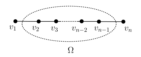
Figure 1.

For convenience, we need the following notion.

Definition 4.1.

For any $f\in\mathbb{R}^{\delta\Omega}$, we call $k\in{\mathbb{R}}$ the $L^{1}$-mean value of $f$ over $\delta\Omega$ if $k$ satisfies

$$m(\{x\in\delta\Omega|f(x)\geq k\})\geq\frac{1}{2}m(\delta\Omega)$$

and

$$m(\{x\in\delta\Omega|f(x)\leq k\})\geq\frac{1}{2}m(\delta\Omega).$$

Remark 4.1.

The $L^{1}$-mean value may not be unique in general. For simplicity, we denote by $\overline{f}$ the $L^{1}$-mean value of $f\in{\mathbb{R}}^{\delta\Omega}$.

Lemma 4.1.

$$\operatorname*{arg\,min}_{k\in{\mathbb{R}}}\sum_{x\in\delta\Omega}m_{x}|f(x)-k|=\overline{f},$$

where $\operatorname*{arg\,min}$ denotes the value $k$ at which $\sum_{x\in\delta\Omega}m_{x}|f(x)-k|$ attains the minimum.

Remark 4.2.

(a) For the proof of Lemma 4.1, one refers to e.g. [CSZ15].

(b) From Lemma 4.1, Theorem 1.1 is equivalent to

(4.1) $$h_{E}(\widetilde{\Omega})=\inf_{f\in{\mathbb{R}}^{\overline{\Omega}}}\frac{\sum_{e=\{x,y\}\in E(\Omega,\overline{\Omega})}\mu_{xy}|f(x)-f(y)|}{\sum_{x\in\delta\Omega}m_{x}|f(x)-\overline{f}|}.$$

We will need the following discrete version of Co-area formula. For discrete Co-area formula, see e.g. [Gri09, Lemma 3.3].

Lemma 4.2.

For any $f\in{\mathbb{R}}^{\overline{\Omega}}$, we have

$$\sum_{e=\{x,y\}\in E(\Omega,\overline{\Omega})}\mu_{xy}|f(x)-f(y)|=\int_{-\infty}^{\infty}\sum_{e=\{x,y\}\in E(\Omega,\overline{\Omega}),f(x)<\sigma\leq f(y)}\mu_{xy}d\sigma.$$

Proof.

For any interval $(a,b]$, we denote by $\chi_{(a,b]}$ the characteristic function on $(a,b]$, i.e.

$$\chi_{(a,b]}(x)=\left\{\begin{array}[]{ll}0,&x\notin(a,b],\\ 1,&x\in(a,b].\end{array}\right.$$

$$\int_{-\infty}^{\infty}\sum_{e=\{x,y\}\in E(\Omega,\overline{\Omega}),f(x)<\sigma\leq f(y)}\mu_{xy}d\sigma = \int_{-\infty}^{\infty}\sum_{e=\{x,y\}\in E(\Omega,\overline{\Omega})}\mu_{xy}\chi_{(f(x),f(y)]}(\sigma)d\sigma$$

$$= \sum_{e=\{x,y\}\in E(\Omega,\overline{\Omega})}\mu_{xy}\int_{-\infty}^{\infty}\chi_{(f(x),f(y)]}(\sigma)d\sigma$$

$$= \sum_{e=\{x,y\}\in E(\Omega,\overline{\Omega})}\mu_{xy}|f(x)-f(y)|.$$

∎

Now we are ready to prove Theorem 1.1.

Proof of Theorem 1.1.

From Remark 4.2, it suffices to prove (4.1). Choose $A\subset\overline{\Omega}$ that achieves $h_{E}(\widetilde{\Omega})$, i.e.

$$m(A\cap\delta\Omega)\leq m(A^{\vee}\cap\delta\Omega),\quad h_{E}(\widetilde{\Omega})=\frac{\mu(\partial_{\Omega}A)}{m(A\cap\delta\Omega)}.$$

Set

$$u(x)=\left\{\begin{array}[]{ll}1,&x\in A,\\ 0,&x\in\overline{\Omega}\setminus A.\end{array}\right.$$

We observe that $\overline{u}$, the $L^{1}$-mean value of $u$, is contained in $[0,1]$. To see this, one just need to notice that if $m(A\cap\delta\Omega)=m(A^{\vee}\cap\delta\Omega)$, then $\overline{u}\in[0,1]$; if $m(A\cap\delta\Omega)<m(A^{\vee}\cap\delta\Omega)$, then $\overline{u}=0$.

For any $t\in[0,1]$,

$$\sum_{x\in\delta\Omega}m_{x}|u(x)-t| = \sum_{x\in A\cap\delta\Omega}m_{x}(1-t)+\sum_{x\in A^{\vee}\cap\delta\Omega}m_{x}t$$

$$= m(A\cap\delta\Omega)+t\cdot\left(m(A^{\vee}\cap\delta\Omega)-m(A\cap\delta\Omega)\right)$$

$$\geq m(A\cap\delta\Omega).$$

Hence

$$\frac{\sum_{e=\{x,y\}\in E(\Omega,\overline{\Omega})}\mu_{xy}|u(x)-u(y)|}{\sum_{x\in\delta\Omega}m_{x}|u(x)-\overline{u}|}\leq\frac{\mu(\partial A\cap E(\Omega,\overline{\Omega}))}{m(A\cap\delta\Omega)}=h_{E}(\widetilde{\Omega}).$$

Then it follows that

$$h_{E}(\widetilde{\Omega})\geq\inf_{f\in{\mathbb{R}}^{\overline{\Omega}}}\frac{\sum_{e=\{x,y\}\in E(\Omega,\overline{\Omega})}\mu_{xy}|f(x)-f(y)|}{\sum_{x\in\delta\Omega}m_{x}|f(x)-\overline{f}|}.$$

Now we prove the opposite direction. For any nonconstant function $f\in{\mathbb{R}}^{\overline{\Omega}}$, choose a constant $c$ such that

$$m(\{f<c\}\cap\delta\Omega)\leq m(\{f\geq c\}\cap\delta\Omega),$$

$$m(\{f\leq c\}\cap\delta\Omega)\geq m(\{f>c\}\cap\delta\Omega).$$

Set $g:=f-c$, then we have

$$m(\{g<\sigma\}\cap\delta\Omega)\leq m(\{g\geq\sigma\}\cap\delta\Omega),\quad for\quad\sigma\leq 0$$

and

$$m(\{g<\sigma\}\cap\delta\Omega)\geq m(\{g\geq\sigma\}\cap\delta\Omega),\quad for\quad\sigma>0.$$

For any $\sigma\in{\mathbb{R}}$, set

$$G(\sigma):=\sum_{e=\{x,y\}\in E(\Omega,\overline{\Omega}),g(x)<\sigma\leq g(y)}\mu_{xy}.$$

Then by Lemma 4.2, we have

$$\sum_{e=\{x,y\}\in E(\Omega,\overline{\Omega})}\mu_{xy}|f(x)-f(y)|=\int_{-\infty}^{\infty}G(\sigma)d\sigma.$$

Set $A:=\{g<\sigma\}$ for $\sigma\leq 0$ and $A:=\{g\geq\sigma\}$ for $\sigma>0$. In either case, we have $m(A\cap\delta\Omega)\leq m(A^{\vee}\cap\delta\Omega)$ and

$$G(\sigma)\geq h_{E}(\widetilde{\Omega})\cdot m(A\cap\delta\Omega)=h_{E}(\widetilde{\Omega})\cdot\left\{\begin{array}[]{ll}m(\{g<\sigma\}\cap\Omega),&\text{\ for}\quad\sigma\leq 0,\\ m(\{g\geq\sigma\}\cap\Omega),&\text{\ for}\quad\sigma>0\end{array}\right.$$

by the definition of $h_{E}(\widetilde{\Omega})$. Hence

$$\sum_{e=\{x,y\}\in E(\Omega,\overline{\Omega})}\mu_{xy}|f(x)-f(y)|=\int_{-\infty}^{0}G(\sigma)d\sigma+\int_{0}^{\infty}G(\sigma)d\sigma$$

$$\geq h_{E}(\widetilde{\Omega})\left(\int_{-\infty}^{0}m(\{g<\sigma\}\cap\Omega)d\sigma+\int_{0}^{\infty}m(\{g\geq\sigma\}\cap\Omega)d\sigma\right)$$

$$= h_{E}(\widetilde{\Omega})\left(\int_{-\infty}^{0}m(\{g<\sigma\}\cap\Omega)d\sigma+\int_{0}^{\infty}m(\{g\geq\sigma\}\cap\Omega)d\sigma\right)$$

$$= h_{E}(\widetilde{\Omega})\left(\int_{-\infty}^{0}\sum_{x\in\delta\Omega}\chi_{(g(x),0]}m_{x}d\sigma+\int_{0}^{\infty}\sum_{x\in\delta\Omega}\chi_{(0,g(x)]}m_{x}d\sigma\right)$$

$$= h_{E}(\widetilde{\Omega})\sum_{x\in\delta\Omega}|f(x)-c|m_{x}.$$

Then the other direction follows and we complete the proof of the theorem. ∎

We obtain the following upper bound estimate for $\lambda_{1}(\Omega).$

Proposition 4.2.

Let $G$ be a finite graph and $\Omega\subset V,$ then we have

$$\lambda_{1}(\Omega)\leq 2h_{E}(\widetilde{\Omega}).$$

Proof.

Choose $A\subset\overline{\Omega}$ that achieves $h_{E}(\widetilde{\Omega})$, i.e. $m(A\cap\delta\Omega)\leq\frac{1}{2}m(\delta\Omega)$ and $\frac{\mu(\partial_{\Omega}A)}{m(A\cap\delta\Omega)}=h_{E}(\widetilde{\Omega})$. Set $\varphi(x)\in\mathbb{R}^{\delta\Omega}$ as

$$\varphi(x)=\left\{\begin{array}[]{ll}\frac{1}{m(A\cap\delta\Omega)},&x\in A\cap\delta\Omega,\\ -\frac{1}{m(A^{\vee}\cap\delta\Omega)},&x\in A^{\vee}\cap\delta\Omega.\end{array}\right.$$

Similarly set $\widetilde{\varphi}(x)$ to be

$$\widetilde{\varphi}(x)=\left\{\begin{array}[]{ll}\frac{1}{m(A\cap\delta\Omega)},&x\in A,\\ -\frac{1}{m(A^{\vee}\cap\delta\Omega)},&x\in A^{\vee}.\end{array}\right.$$

Then we have

$$\lambda_{1}(\Omega) \leq \frac{D_{\Omega}(u_{\varphi})}{\sum_{x\in\delta\Omega}\varphi^{2}(x)m_{x}}\leq\frac{D_{\Omega}(\widetilde{\varphi})}{\sum_{x\in\delta\Omega}\varphi^{2}(x)m_{x}}$$

$$= \left(\frac{1}{m(A\cap\delta\Omega)}+\frac{1}{m(A^{\vee}\cap\delta\Omega)}\right)\mu(\partial A\cap E(\Omega,\overline{\Omega}))$$

$$\leq 2\frac{\mu(\partial_{\Omega}A)}{m(A\cap\delta\Omega)}=2h_{E}(\widetilde{\Omega}).$$

The second inequality follows from the fact that harmonic functions minimize the Dirichlet energy among functions with the same boundary condition. ∎

Figure 2.

Remark 4.3.

The above upper bound estimate for $\lambda_{1}(\Omega)$ is sharp. From the following example, we can see that the factor 2 in the upper bound estimate can’t be reduced.

Example 4.2.

Consider a sequence of graphs $\{G_{n}\}_{n=1}^{\infty}$ as shown in Figure 2 with $\Omega_{n}=\{w_{1},w_{2}\}$, $\delta\Omega_{n}=\{v_{1},v_{2},\cdots,v_{4n}\}$ and unit edge weights. By calculation, $\lambda_{1}(G_{n})=\frac{1}{n+1}$ and $h_{E}(G_{n})=\frac{1}{2n}$. Hence $\lambda_{1}(G_{n})=\frac{1}{n+1}\leq\frac{1}{n}=2h_{E}(G_{n}).$

At the end of this section, we give the proof of Theorem 1.2.

Proof of Theorem 1.2.

Let $u$ be the first eigenvector associated to $\lambda_{1}(\Omega)$. For simplicity, we still denote by $u$ the harmonic extension of $u$. Set $v=(u-\overline{u})_{+}$ and choose $\overline{v}=0$. Then

$$m(\{v=0\}\cap\delta\Omega)\geq\frac{1}{2}m(\delta\Omega).$$

Applying Theorem 1.1 by choosing $f=v^{2}$, we have

$$h_{E}(\widetilde{\Omega})\cdot\sum_{x\in\delta\Omega}v^{2}(x)m_{x}\leq\sum_{e=\{x,y\}\in E(\Omega,\overline{\Omega})}\mu_{xy}|v^{2}(x)-v^{2}(y)|.$$

For the right hand side of the above inequality,

$$\left(\sum_{e=\{x,y\}\in E(\Omega,\overline{\Omega})}\mu_{xy}\left|v^{2}(x)-v^{2}(y)\right|\right)^{2}$$

$$\leq \sum_{e=\{x,y\}\in E(\Omega,\overline{\Omega})}\mu_{xy}(v(x)+v(y))^{2}\cdot\sum_{e=\{x,y\}\in E(\Omega,\overline{\Omega})}\mu_{xy}(v(x)-v(y))^{2}$$

$$\leq 2\sum_{e=\{x,y\}\in E(\Omega,\overline{\Omega})}\mu_{xy}(v^{2}(x)+v^{2}(y))\cdot\sum_{e=\{x,y\}\in E(\Omega,\overline{\Omega})}\mu_{xy}(v(x)-v(y))^{2}.$$

Notice that it suffices to consider the graph $\widetilde{\Omega}$, then

$$\sum_{e=\{x,y\}\in E(\Omega,\overline{\Omega})}\mu_{xy}(v^{2}(x)+v^{2}(y))$$

$$= \frac{1}{2}\sum_{x,y\in\Omega}\mu_{xy}(v^{2}(x)+v^{2}(y))+\sum_{x\in\Omega}\sum_{y\in\delta\Omega}\mu_{xy}(v^{2}(x)+v^{2}(y))$$

$$= \sum_{x\in\Omega}v^{2}(x)\left(\sum_{y\in\Omega}+\sum_{y\in\delta\Omega}\right)\mu_{xy}+\sum_{y\in\delta\Omega}v^{2}(y)\sum_{x\in\Omega}\mu_{xy}$$

$$= \sum_{x\in\overline{\Omega}}v^{2}(x)m_{x}.$$

Hence

$$h_{E}(\widetilde{\Omega})\cdot\sum_{x\in\delta\Omega}v^{2}(x)m_{x}\leq\left(2\sum_{x\in\overline{\Omega}}v^{2}(x)m_{x}\cdot\!\!\!\!\sum_{e=\{x,y\}\in E(\Omega,\overline{\Omega})}\!\!\mu_{xy}(v(x)-v(y))^{2}\right)^{1/2},$$

i.e.

$$h_{E}(\widetilde{\Omega})\cdot\sum_{x\in\delta\Omega}(u-\overline{u})^{2}_{+}m_{x}\leq\left(2\sum_{x\in\overline{\Omega}}(u-\overline{u})^{2}_{+}m_{x}\cdot\sum_{e=\{x,y\}\in E(\Omega,\overline{\Omega})}\mu_{xy}(u(x)-u(y))^{2}\right)^{1/2}.$$

Similarly, we have

$$h_{E}(\widetilde{\Omega})\cdot\sum_{x\in\delta\Omega}(u-\overline{u})^{2}_{-}m_{x}\leq\left(2\sum_{x\in\overline{\Omega}}(u-\overline{u})^{2}_{-}m_{x}\cdot\sum_{e=\{x,y\}\in E(\Omega,\overline{\Omega})}\mu_{xy}(u(x)-u(y))^{2}\right)^{1/2}.$$

Hence

$$h_{E}(\widetilde{\Omega})\cdot\sum_{x\in\delta\Omega}(u-\overline{u})^{2}m_{x}$$

$$\leq \left(2\sum_{x\in\overline{\Omega}}(u-\overline{u})^{2}m_{x}\cdot\sum_{e=\{x,y\}\in E(\Omega,\overline{\Omega})}\mu_{xy}(u(x)-u(y))^{2}\right)^{1/2}$$

$$\leq \frac{a}{2}\sum_{x\in\overline{\Omega}}(u-\overline{u})^{2}m_{x}+\frac{1}{a}\sum_{e=\{x,y\}\in E(\Omega,\overline{\Omega})}\mu_{xy}(u(x)-u(y))^{2}$$

$$= \frac{a}{2}\left(\sum_{x\in\Omega}+\sum_{x\in\delta\Omega}\right)(u-\overline{u})^{2}m_{x}+\frac{1}{a}\sum_{e=\{x,y\}\in E(\Omega,\overline{\Omega})}\mu_{xy}(u(x)-u(y))^{2}.$$

For any $\varphi\in\mathds{R}^{\overline{\Omega}}$ we have

$$\mu_{1}(k)\leq\frac{D_{\Omega}(\varphi)+k\sum_{x\in\delta\Omega}\varphi^{2}(x)m_{x}}{\sum_{x\in\Omega}\varphi^{2}(x)m_{x}}.$$

Hence

$$\sum_{x\in\Omega}(u-\overline{u})^{2}m_{x}\leq\frac{D_{\Omega}(u)}{\mu_{1}(k)}+\frac{k}{\mu_{1}(k)}\sum_{x\in\delta\Omega}(u-\overline{u})^{2}m_{x}.$$

Combining with the above inequality and (LABEL:1), we have

$$\left(h_{E}(\widetilde{\Omega})-\frac{a(k+\mu_{1}(k))}{2\mu_{1}(k)}\right)\frac{2a\mu_{1}(k)}{a^{2}+2\mu_{1}(k)}\leq\frac{D_{\Omega}(u)}{\sum_{x\in\delta\Omega}(u-\overline{u})^{2}m_{x}}.$$

Using the fact that $u$ is the first eigenfunction associated to $\lambda_{1}$ we find that

$$\left(h_{E}(\widetilde{\Omega})-\frac{a(k+\mu_{1}(k))}{2\mu_{1}(k)}\right)\frac{2a\mu_{1}(k)}{a^{2}+2\mu_{1}(k)}\leq\frac{\lambda_{1}\sum_{x\in\delta\Omega}u^{2}(x)m_{x}}{\sum_{x\in\delta\Omega}(u-\overline{u})^{2}m_{x}}.$$

Since $\langle u,1\rangle_{\delta\Omega}=0$, we have

$$\frac{\sum_{x\in\delta\Omega}u^{2}(x)m_{x}}{\sum_{x\in\delta\Omega}(u-\overline{u})^{2}m_{x}}\leq 1$$

and therefore

$$\lambda_{1}(\Omega) \geq \left(h_{E}(\widetilde{\Omega})-\frac{a(k+\mu_{1}(k))}{2\mu_{1}(k)}\right)\frac{2a\mu_{1}(k)}{a^{2}+2\mu_{1}(k)}$$

$$= \frac{\left(2h_{E}(\widetilde{\Omega})\mu_{1}(k)-a(k+\mu_{1}(k))\right)a}{a^{2}+2\mu_{1}(k)}.$$

∎

Remark 4.4.

The maximum of the right hand side of (1.2) with respect to $a$ can be achieved at

$$a_{0}=\frac{2h\mu}{\sqrt{(k+\mu)^{2}+2h^{2}\mu}+(k+\mu)}$$

and the maximum is

$$\frac{h^{2}\mu\sqrt{(k+\mu)^{2}+2h^{2}\mu}}{2h^{2}\mu+(k+\mu)^{2}+(k+\mu)\sqrt{(k+\mu)^{2}+2h^{2}\mu}}.$$

5. Jammes-type Cheeger estimate

Proposition 5.1.

Let $G$ be a finite graph and $\Omega\subset V$, then we have

$$h_{J}(\widetilde{\Omega})\leq 1.$$

Proof.

Choose $A=\{v\},$ where $v\in\delta\Omega$. Then by the definition of $h_{J}(\widetilde{\Omega})$, we have $h_{J}(\widetilde{\Omega})\leq\frac{\mu(\partial_{\Omega}A)}{m(A\cap\delta\Omega)}=\frac{m_{v}}{m_{v}}=1$. ∎

The eigenvalues of $\Lambda$ can be characterised by Rayleigh quotient as follows

$$\lambda_{1}(\Omega)=\inf_{\varphi\in{\mathbb{R}}^{\delta\Omega},\|\varphi\|_{\ell^{2}}=1,\varphi\perp 1}\langle\Lambda\varphi,\varphi\rangle=\inf_{\varphi\in{\mathbb{R}}^{\delta\Omega},\|\varphi\|_{\ell^{2}}=1,\varphi\perp 1}D_{\Omega}(u_{\varphi}),$$

$$\lambda_{N-1}(\Omega)=\sup_{\varphi\in{\mathbb{R}}^{\delta\Omega},\|\varphi\|_{\ell^{2}}=1}\langle\Lambda\varphi,\varphi\rangle=\sup_{\varphi\in{\mathbb{R}}^{\delta\Omega},\|\varphi\|_{\ell^{2}}=1}D_{\Omega}(u_{\varphi}).$$

We denote by $\sigma_{1}$ the first nontrivial eigenvalue of the Dirichlet-to-Neumann operator on a compact manifold with boundary. For convenience, we recall the idea of the proof of Jammes-type Cheeger estimate, which can be divided into four steps.

Step 1: Choosing $f$ as the eigenfunction associated to $\sigma_{1}$, we still denote by $f$ the harmonic extension of $f$ to $M$ with ${\mathrm{vol}}(M^{+})\leq\frac{{\mathrm{vol}}(M)}{2}$, where $M^{+}:=\{x\in M|f(x)>0\}$.

Step 2: Show that $\sigma_{1}=\frac{\int_{M^{+}}|df|^{2}}{\int_{\partial M^{+}}f^{2}}$, where $\partial M^{+}=M^{+}\cap\partial M.$

Step 3: By Hölder’s inequality, $\sigma_{1}=\frac{(\int_{M^{+}}f^{2})(\int_{M^{+}}|df|^{2})}{(\int_{M^{+}}f^{2})(\int_{\partial M^{+}}f^{2})}\geq\frac{1}{4}\frac{(\int_{M^{+}}|d(f^{2})|)^{2}}{(\int_{M^{+}}f^{2})(\int_{\partial M^{+}}f^{2})}$.

Step 4: Set $D_{t}:=f^{-1}([\sqrt{t},\infty))$, $\partial_{I}D_{t}:=\partial D_{t}\cap\mathrm{int}(M)$ and $\partial_{E}D_{t}:=\partial D_{t}\setminus\partial_{I}D_{t}$. Use Co-area formula to show that $\int_{M^{+}}|d(f^{2})|=\int_{t\geq 0}\mathrm{Area}(\partial_{I}D_{t})$, $\int_{M^{+}}f^{2}=\int_{t\geq 0}{\mathrm{vol}}(D_{t})$ and $\int_{\partial M^{+}}f^{2}=\int_{t\geq 0}\mathrm{Area}(\partial_{E}D_{t})$.

Then by the definitions of $h_{M}$ and $h_{J}(M)$ the lower bound estimate of $\sigma_{1}$ follows.

Inspired by the Riemannian case, we can prove the Jammes-type Cheeger constant for $\lambda_{1}(\Omega)$ in the discrete setting. Let $0\neq f\in{\mathbb{R}}^{\delta\Omega}$ be an eigenfunction associated to $\lambda_{1}(\Omega)$. For convenience, we still denote $u_{f}$ by $f(x)$. Set $\overline{\Omega}^{+}=\{x\in\overline{\Omega}\mid f(x)>0\}$ with $m(\overline{\Omega}^{+})\leq\frac{m(\overline{\Omega})}{2}$ (otherwise we can change the sign of $f$) and set

(5.1) $$g(x)=\left\{\begin{array}[]{ll}f(x),&x\in\overline{\Omega}^{+},\\ 0,&otherwise.\end{array}\right.$$

For simplicity, we set $\overline{\Omega}^{-}:=\overline{\Omega}\setminus\overline{\Omega}^{+}$, $\Omega^{+}:=\overline{\Omega}^{+}\cap\Omega$, $\Omega^{-}:=\Omega\setminus\Omega^{+}$, $\delta^{+}\Omega:=\overline{\Omega}^{+}\cap\delta\Omega$ and $\delta^{-}\Omega:=\delta\Omega\setminus\delta^{+}\Omega$. In order to prove Jammes-type Cheeger estimate, we need the following Lemmas.

Lemma 5.1.

For $g$ as in (5.1), we have

(5.2) $$\lambda_{1}(\Omega)\geq\frac{\sum_{e=\{x,y\}\in E(\overline{\Omega}^{+},\overline{\Omega})}\mu_{xy}(g(y)-g(x))^{2}}{\sum_{x\in\delta^{+}\Omega}g^{2}(x)m_{x}}.$$

Proof.

Notice that it suffices to consider graph $\widetilde{\Omega}$. Hence for any $x\in\delta\Omega$, we have

$$\Delta f(x)=\frac{1}{m_{x}}\sum_{y\in\Omega}\mu_{xy}(f(y)-f(x))=-\frac{\partial f(x)}{\partial n}.$$

Then

(5.3) $$\langle\Delta f(x),g(x)\rangle_{\overline{\Omega}^{+}} = \sum_{x\in\Omega^{+}}\Delta f(x)g(x)m_{x}+\sum_{x\in\delta^{+}\Omega}\Delta f(x)g(x)m_{x}$$

$$= -\lambda_{1}(\Omega)\sum_{x\in\delta^{+}\Omega}g^{2}(x)m_{x}.$$

Notice that

$$\langle\Delta f(x),g(x)\rangle_{\overline{\Omega}^{+}}=\left(\sum_{x\in\overline{\Omega}^{+}}\sum_{y\in\overline{\Omega}^{+}}+\sum_{x\in\overline{\Omega}^{+}}\sum_{y\in\overline{\Omega}^{-}}\right)\mu_{xy}(f(y)-f(x))g(x)$$

$$= -\frac{1}{2}\sum_{x,y\in\overline{\Omega}^{+}}\mu_{xy}(f(y)-f(x))(g(y)-g(x))-\sum_{x\in\overline{\Omega}^{+}}\sum_{y\in\overline{\Omega}^{-}}\mu_{xy}(f(x)-f(y))(g(x)-g(y))$$

$$\leq -\sum_{e=\{x,y\}\in E(\overline{\Omega}^{+},\overline{\Omega}^{+})}\mu_{xy}(g(y)-g(x))^{2}-\sum_{x\in\overline{\Omega}^{+}}\sum_{y\in\overline{\Omega}^{-}}\mu_{xy}(g(x)-g(y))^{2}$$

$$= -\sum_{e=\{x,y\}\in E(\overline{\Omega}^{+},\overline{\Omega})}\mu_{xy}(g(y)-g(x))^{2}.$$

Then the lemma follows in view of (5.3). ∎

Multiplying both the numerator and denominator of the fraction in the right hand side of (5.2) by $\sum_{x\in\overline{\Omega}^{+}}g^{2}(x)m_{x}$ and setting

$$\frac{P}{Q}:=\frac{\sum_{x\in\overline{\Omega}^{+}}g^{2}(x)m_{x}\cdot\sum_{e=\{x,y\}\in E(\overline{\Omega}^{+},\overline{\Omega})}\mu_{xy}(g(y)-g(x))^{2}}{\sum_{x\in\overline{\Omega}^{+}}g^{2}(x)m_{x}\cdot\sum_{x\in\delta^{+}\Omega}g^{2}(x)m_{x}},$$

we have

(5.4) $$\lambda_{1}(\Omega)\geq\frac{P}{Q}.$$

Lemma 5.2.

$$P\geq\frac{1}{2}\left(\sum_{e=\{x,y\}\in E(\overline{\Omega}^{+},\overline{\Omega})}|g^{2}(x)-g^{2}(y)|\mu_{xy}\right)^{2}.$$

Proof.

Note that

$$\sum_{x\in\overline{\Omega}^{+}}g^{2}(x)m_{x}=\left(\sum_{x\in\overline{\Omega}^{+}}\sum_{y\in\overline{\Omega}^{+}}+\sum_{x\in\overline{\Omega}^{+}}\sum_{y\in\overline{\Omega}^{-}}\right)g^{2}(x)\mu_{xy}$$

$$= \frac{1}{2}\sum_{x,y\in\overline{\Omega}^{+}}(g^{2}(x)+g^{2}(y))\mu_{xy}+\sum_{x\in\overline{\Omega}^{+}}\sum_{y\in\overline{\Omega}^{-}}g^{2}(x)\mu_{xy}$$

$$= \sum_{e=\{x,y\}\in E(\overline{\Omega}^{+},\overline{\Omega}^{+})}(g^{2}(x)+g^{2}(y))\mu_{xy}+\sum_{x\in\overline{\Omega}^{+}}\sum_{y\in\overline{\Omega}^{-}}g^{2}(x)\mu_{xy}$$

$$= \sum_{e=\{x,y\}\in E(\overline{\Omega}^{+},\overline{\Omega})}(g^{2}(x)+g^{2}(y))\mu_{xy}.$$

Hence

$$P = \sum_{e=\{x,y\}\in E(\overline{\Omega}^{+},\overline{\Omega})}(g^{2}(x)+g^{2}(y))\mu_{xy}\cdot\sum_{e=\{x,y\}\in E(\overline{\Omega}^{+},\overline{\Omega})}\mu_{xy}(g(y)-g(x))^{2}$$

$$\geq \frac{1}{2}\sum_{e=\{x,y\}\in E(\overline{\Omega}^{+},\overline{\Omega})}(g(x)+g(y))^{2}\mu_{xy}\cdot\sum_{e=\{x,y\}\in E(\overline{\Omega}^{+},\overline{\Omega})}\mu_{xy}(g(y)-g(x))^{2}$$

$$\geq \frac{1}{2}\left(\sum_{e=\{x,y\}\in E(\overline{\Omega}^{+},\overline{\Omega})}|g^{2}(x)-g^{2}(y)|\mu_{xy}\right)^{2}.$$

The last inequality follows from Hölder’s inequality. ∎

For any $t>0$, set $D_{t}:=g^{-1}([\sqrt{t},+\infty))=\{x\in\overline{\Omega}|g^{2}(x)\geq t\}$. Then we have $m(D_{t})\leq m(\overline{\Omega}^{+})\leq\frac{m(\overline{\Omega})}{2}$.

Lemma 5.3.

$$\int_{0}^{\infty}\mu(\partial D_{t}\cap E(\Omega,\overline{\Omega}))dt=\sum_{e=\{x,y\}\in E(\overline{\Omega}^{+},\overline{\Omega})}\mu_{xy}|g^{2}(x)-g^{2}(y)|.$$

Proof.

It follows from Lemma 4.2 by setting $f=g^{2}$ and considering the edge set $E(\overline{\Omega}^{+},\overline{\Omega})$. ∎

Lemma 5.4.

$$\int_{0}^{\infty}m(D_{t})dt=\sum_{x\in\overline{\Omega}^{+}}g^{2}(x)m_{x}.$$

$$\int_{0}^{\infty}m(D_{t}\cap\delta\Omega)dt=\sum_{x\in\delta^{+}\Omega}g^{2}(x)m_{x}.$$

Proof.

Similar to Lemma 4.2, we have

$$\int_{0}^{\infty}m(D_{t})dt=\int_{0}^{\infty}\sum_{x\in D_{t}}m_{x}dt=\int_{0}^{\infty}\sum_{x\in\overline{\Omega}^{+}}m_{x}\chi_{(0,g^{2}(x)]}(t)dt=\sum_{x\in\overline{\Omega}^{+}}g^{2}(x)m_{x}$$

and

$$\int_{0}^{\infty}m(D_{t}\cap\delta\Omega)dt=\int_{0}^{\infty}\sum_{x\in\delta^{+}\Omega}m_{x}\chi_{(0,g^{2}(x)]}(t)dt=\sum_{x\in\delta^{+}\Omega}g^{2}(x)m_{x}.$$

∎

Now we are ready to prove Theorem 1.3.

Proof of Theorem 1.3.

Combining with the above Lemmas (Lemma 5.1 to 5.4), we have

$$\lambda_{1}(\Omega) \geq \frac{1}{2}\frac{\int_{0}^{\infty}\mu(\partial D_{t}\cap E(\Omega,\overline{\Omega}))dt\cdot\int_{0}^{\infty}\mu(\partial D_{t}\cap E(\Omega,\overline{\Omega}))dt}{\sum_{x\in\overline{\Omega}^{+}}g^{2}(x)m_{x}\cdot\sum_{x\in\delta^{+}\Omega}g^{2}(x)m_{x}}$$

$$\geq \frac{1}{2}\frac{\int_{0}^{\infty}h(\widetilde{\Omega})m(D_{t})dt\cdot\int_{0}^{\infty}h_{J}(\widetilde{\Omega})m(D_{t}\cap\delta\Omega)dt}{\sum_{x\in\overline{\Omega}^{+}}g^{2}(x)m_{x}\cdot\sum_{x\in\delta^{+}\Omega}g^{2}(x)m_{x}}$$

$$= \frac{h(\widetilde{\Omega})h_{J}(\widetilde{\Omega})}{2}\frac{\int_{0}^{\infty}m(D_{t})dt\cdot\int_{0}^{\infty}m(D_{t}\cap\delta\Omega)dt}{\sum_{x\in\overline{\Omega}^{+}}g^{2}(x)m_{x}\cdot\sum_{x\in\delta^{+}\Omega}g^{2}(x)m_{x}}$$

$$= \frac{h(\widetilde{\Omega})h_{J}(\widetilde{\Omega})}{2}.$$

∎

From Theorem 1.3, we know that $h(\widetilde{\Omega})$ plays an important role in Jammes-type Cheeger estimate. Recall that $\zeta_{1}(\widetilde{\Omega})$ is the first nontrivial eigenvalue of the Laplace operator with no boundary condition on $\widetilde{\Omega}$ and the classical Cheeger estimates reads as

(5.5) $$2h(\widetilde{\Omega})\geq\zeta_{1}(\widetilde{\Omega})\geq\frac{h(\widetilde{\Omega})^{2}}{2},$$

see [Chu97, p.26]. Then we are ready to prove Corollary 1.1

Proof of Corollary 1.1.

Recall that $h(\widetilde{\Omega})\leq h_{J}(\widetilde{\Omega})$. Combining with Theorem 1.3 and (5.5), we have

(5.6) $$\lambda_{1}(\Omega)\geq\frac{h(\widetilde{\Omega})^{2}}{2}\geq\frac{(\zeta_{1}(\widetilde{\Omega}))^{2}}{8}.$$

∎

Finally we give an example to show that $\lambda_{1}$ can’t be bounded from below using only $h_{J}(\widetilde{\Omega})$.

Example 5.1.

Consider a path graph with even vertices n ($n\geq 6$) and unit edge weights as shown in Figure 1. Set $\Omega=\{v_{2},v_{3},\cdots,v_{n-1}\}$, $\delta_{E}\Omega=\{v_{1},v_{n}\}$. Then we have

$$\Lambda=\left(\begin{array}[]{cc}\frac{1}{n-1}&-\frac{1}{n-1}\\ -\frac{1}{n-1}&\frac{1}{n-1}\end{array}\right).$$

Hence $\lambda_{0}(\Omega)=0$ and $\lambda_{1}(\Omega)=\frac{2}{n-1}$. Choosing $A=\{v_{1},v_{2},\cdots,v_{\frac{n}{2}}\}$, we obtain that $h(\widetilde{\Omega})=\frac{1}{n-1}$ and $h_{J}(\widetilde{\Omega})=1$. Hence the Jammes-type Cheeger estimate we obtained is asymptotically sharp of the same order $\frac{1}{n-1}$ on both sides as $n\rightarrow\infty$. Moreover, one can not obtain that $\lambda_{1}(\Omega)\geq F(h_{J}(\widetilde{\Omega}))$ for any positive function $F$.