A common-envelope wind model for Type Ia supernovae (I): binary evolution and birth rate

Abstract

The single-degenerate (SD) model is one of the principal models for the progenitors of type Ia supernovae (SNe Ia), but some of the predictions in the most widely studied version of the SD model, i.e. the optically thick wind (OTW) model, have not been confirmed by observations. Here, we propose a new version of the SD model in which a common envelope (CE) is assumed to form when the mass-transfer rate between a carbon-oxygen white dwarf (CO WD) and its companion exceeds a critical accretion rate. The WD may gradually increase its mass at the base of the CE. Due to the large nuclear luminosity for stable hydrogen burning, the CE may expand to giant dimensions and will lose mass from the surface of the CE by a CE wind (CEW). Because of the low CE density, the binary system will avoid a fast spiral-in phase and finally re-emerge from the CE phase. Our model may share the virtues of the OTW model but avoid some of its shortcomings. We performed binary stellar evolution calculations for more than 1100 close WD + MS binaries. Compared with the OTW model, the parameter space for SNe Ia from our CEW model extends to more massive companions and less massive WDs. Correspondingly, the Galactic birth rate from the CEW model is higher than that from the OTW model by $\sim$30%. Finally, we discuss the uncertainties of the CEW model and the differences between our CEW model and the OTW model.

1 Introduction

Being an excellent cosmological distance indicators, Type Ia supernovae (SNe Ia) have been successfully applied to determine cosmological parameters (e.g. $\Omega$ and $\Lambda$; Riess et al. 1998; Perlmutter et al. 1999). Indeed it has even been proposed that SNe Ia can be used for testing the evolution of the equation of the state of dark energy with time (Howell et al. 2009). SNe Ia also play an important part in understanding the role of galactic chemical evolution as they are believed to be the main producer of iron in their host galaxies (Greggio & Renzini 1983; Matteucci & Greggio 1986). They are also accelerators of cosmic rays and sources of kinetic energy in galaxy evolution processes (Helder et al. 2009; Powell et al. 2011).

It is widely accepted that SNe Ia originate from the thermonuclear runaway of a carbon-oxygen white dwarf (CO WD) in a binary system. The CO WD accretes material from its companion, increases mass to its maximum stable mass, and then explodes as a thermonuclear runaway. Almost half of the WD mass is converted into radioactive ⁵⁶Ni during the explosion (Branch 2004), and the amount of ⁵⁶Ni determines the maximum luminosity of SNe Ia (Arnett 1982). However, the precise nature of the progenitor systems remains unclear (Branch et al. 1995; Hillebrandt & Niemeyer 2000; Leibundgut 2000; Maoz, Mannucci & Nelemans 2014), although the identification of the progenitor has wide-ranging implications in a number of related astrophysical fields (Wang & Han 2012; Meng et al. 2015). There have been two main competing scenarios for the last 4 decades for the progenitor systems of SNe Ia, which depend on the nature of the companion star. In the single-degenerate (SD) model, a CO WD grows in mass by accretion from its non-degenerate companion (Whelan & Iben 1973; Nomoto, Thielemann & Yokoi 1984) while, in the double degenerate (DD) scenario, two WDs merge after losing angular momentum by gravitational-wave radiation (Iben & Tutukov 1984; Webbink 1984). There is some support for both models, but there also are some serious problems, both on the observational as well as the theoretical side (Howell 2011; Maoz, Mannucci & Nelemans 2014). In this paper, we focus on the SD model.

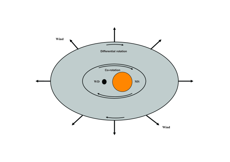
Figure 1: Schematic diagram illustrating the CE-wind model. The mass-transfer rate from the Roche-lobe filling companion exceeds the critical accretion rate at which the WD can accrete. This leads to the formation of a common envelope (CE). The inner region of the CE co-rotates with the binary, while the outer region rotates differentially. Mass is lost from the surface of the CE, powered in part by the luminosity emitted from the accreting WD and in part by the frictional energy generated in the differentially rotating region.

In the standard SD model, the maximum stable mass of a CO WD is close to the Chandrasekhar mass ($\sim 1.378\,M_{\odot}$, Nomoto, Thielemann & Yokoi 1984). The companion of the WD may be a main sequence star or a sub-giant star (WD+MS), or a red-giant star (WD+RG) (Yungelson et al. 1995; Li & van den Heuvel 1997; Nomoto et al. 1999; Hachisu et al. 1999a, b; Langer et al. 2000; Han & Podsiadlowski 2004). There is substantial observational support for the SD model: e.g., the detection of circumstellar material (CSM) in the spectrum of SNe Ia is usually taken as strong evidence in favor of the SD model (Patat et al. 2007; Sternberg et al. 2011; Dilday et al. 2012; Maguire et al. 2013). Moreover, supersoft X-ray sources (SSSs, WD + MS or WD + RG systems, van den Heuvel 1992; Di Stefano & Kong 2003) have been proposed to be good candidates as the progenitors of SNe Ia (Hachisu & Kato 2003a, b). Recently, the UV excesses expected from the collision between supernova ejecta and their companion have been reported, which provides fairly definitive support for the SD model at least in these cases (Kasen 2010; Foley et al. 2012; Brown 2014; Cao et al. 2015, 2016; Marion et al. 2016; Graur et al. 2016). It is therefore quite possible that all SN 2002es-like supernovae arise from SD systems (Cao et al. 2016). A direct method for confirming this type of progenitor model is to search for the companion stars of SNe Ia in their remnants. The claimed discovery of a potential companion of Tycho’s supernova could in principle support the WD + MS model (Ruiz-Lapuente et al. 2004; González-Hernández et al. 2009; Bedin et al. 2014), although there are some strong doubts about this identification (Kerzendorf et al. 2009, 2013). Here, we concentrate on the WD + MS channel, which is likely to be a very important channel for producing SNe Ia in our Galaxy and other late-type galaxies (Han & Podsiadlowski 2004).

Whether a CO WD explodes as a SN Ia in the SD model depends mainly on the mass-transfer rate from its companion. The maximum accretion rate for stable hydrogen burning on a WD surface defines a critical accretion rate, $\dot{M}_{\rm cr}$ (Nomoto 1982; Nomoto et al. 2007). If the mass-transfer rate is larger than $\dot{M}_{\rm cr}$, the WD may expand to become a RG-like object, and then a common envelope (CE) may form which engulfs both the WD and its companion. In the past it had been suggested that the system would then experience a spiral-in phase where the system will ultimately merge and avoid a SN Ia (Nomoto et al. 1979); this is one of the reasons for the low birth rate of SNe Ia from the SD model. To avoid this problem, the optically thick wind (OTW) model was proposed (Hachisu et al. 1996; Hachisu et al. 1999a, b), in which the accreted hydrogen steadily burns on the surface of the WD at the rate $\dot{M}_{\rm cr}$ while the unprocessed matter is lost from the system as an OTW. Since Hachisu et al. (1996), many studies have been based on the OTW model (Li & van den Heuvel 1997; Han & Podsiadlowski 2004; Chen & Li 2007; Hachisu et al. 2008; Meng et al. 2009a; Meng & Yang 2010a; Wang, Li & Han 2010; Chen et al. 2011; Hachisu et al. 2012). The OTW helps to modify the mass-growth rate of the WD and the mass-transfer rate to avoid the formation of a CE, increasing the birth rate of SNe Ia significantly (Han & Podsiadlowski 2004). The OTW model may also explain the properties of SSSs and recurrent novae (RN, Hachisu & Kato 2003a, b; Hachisu & Kato 2005, 2006a, 2006b; Hachisu et al. 2007).

However, some of the predictions of the model are in conflict with observations. According to the opacity calculations by Iglesias & Rogers (1996), whether the OTW may occur or not is heavily dependent on the Fe abundance. When $Z$ is lower than $0.002$, it is found that the opacity is too low to drive a wind, i.e. no OTW occurs (Kobayashi et al. 1998). This implies that there exists a low-metallicity threshold for SNe Ia in contrast to SNe II. However, no such metallicity threshold has been found in galaxy host studies (Prieto et al. 2008; Galbany et al. 2016). For the same reason, SNe Ia are not expected at high redshift ($z>1.4$, Kobayashi et al. 1998), but recently a SN Ia at $z=2.26$ was reported (Rodney et al. 2015). Furthermore, some other SNe Ia at high redshift and/or in low-metallicity environments have also been discovered (Rodney et al. 2012; Frederiksen et al. 2012; Jones et al. 2013). The material lost from the binary system in the OTW will shape the CSM around the SN Ia; because of the large wind velocity ($\sim 1000\,{\rm kms^{\rm-1}}$), it may create a low-density bubble or wind-blown cavity around the SN Ia. Its modification of the CSM on larger scales could become apparent during the SNR phase. Badenes et al. (2007) tried to search for the signatures of wind-blown cavities in seven young SN Ia remnants that would be expected in the OTW model. Unfortunately, they found that such large cavities are incompatible with the dynamics of the forward shock and the X-ray emission from the shocked ejecta in all seven SN Ia remnants. This result may indicate that the progenitors do not modify their surroundings in a strong way – especially, the absorption features seen in the spectra of SNe Ia suggest small cavities of radius $\sim 10^{\rm 17}$ cm (Patat et al. 2007; Blondin et al. 2009; Borkowskin et al. 2009; Simon et al. 2009; Sternberg et al. 2011; Patnaude et al. 2012). In addition, by modelling two remnants in the Large Magellanic Cloud with strong Fe-L line emission in their interiors, Borkowskin et al. (2006) found that the two remnants required a large interior density, which would be expected from a low-velocity pre-explosion wind rather than the fast OTW.

As an alternative, a super-Eddington-wind (SEW) scenario has been suggested which only weakly depends on metallicity (Ma et al. 2013). However, this model also has the wind velocity problem. In addition, whatever in SEW model or in OTW model, there is a fine-tuning problem that how the helium flash and hydrogen burning adjust with each other (e.g. Piersanti et al. 2000; Shen & Bildsten 2007; Woosley & Kasen 2011). This issue is crucial to determine whether or not a CO WD may effectively increase its mass.

Figure 2: An example of the evolution of a binary in the CEW model. The evolution of various parameters are shown, including the CO WD mass, $M_{\rm WD}$, the secondary mass, $M_{\rm 2}$, the mass-transfer rate, $\dot{M}_{\rm 2}$, the mass-growth rate of the CO WD, $\dot{M}_{\rm WD}$, the mass of the CE, $M_{\rm CE}$, the mass-loss rate from the system, $\dot{M}_{\rm loss}$, the frictional luminosity, $L_{\rm f}$, and the merger timescale for the binary system, $I/\dot{I}$, as labelled in each panel. The evolutionary tracks of the donor stars are shown as solid curves and the evolution of the orbital periods is shown as dashed curves in panel (1). Dotted vertical lines in all panels and asterisks in panel (1) indicate the position where the WD is expected to explode as a SN Ia. The initial binary parameters and the binary parameters at the time of the SN Ia explosion are also given in panel (1).

If there is no OTW or SEW, the status of the SD model goes back to the situation some 20 years ago. However, whether the formation of a CE really needs to be avoided, as suggested by Nomoto et al. (1979), has never been properly addressed. In this paper, we constructed a new SD model in which no OTW occurs but a CE forms around the binary systems when the mass-transfer rate exceeds the critical accretion rate. As we will show, a CE does not generally lead to the merger of the binary system as the density in the CE is usually quite low, resulting in a long spiral-in timescale. Indeed the existence of a temporary CE has many attractive features: the WD will naturally grow at the stable nuclear burning rate, both for H and He shell burning phases (similar to the situation in thermally pulsing asymptotic giant branch [TPAGB] stars), avoiding some of the fine-tuning in the classical SD model. While the CE acts as a mass reservoir, the wind from an extended CE envelope will naturally produce the low velocities in the circumstellar medium (CSM) as inferred for some SNe Ia (Badenes et al. 2007; Patat et al. 2007). As the system will have the appearance of a TPAGB star in the main WD accretion phase, no X-rays are expected, alleviating the existing X-ray constraints on the SD model (Gilfanov & Bogdán 2010; Di Stefano 2010). In many cases, some H-rich CE material is still left at the time of the explosion. While, in most cases, this will not be directly detectible, it may explain the high-velocity Ca features observed in many SNe Ia which seem to require the existence of some H (Mazzali et al. 2005a, b).

In this paper we will comprehensibly study this new framework for the SD scenario specifically for the WD + MS channel and systematically determine the parameter space for potential SN Ia progenitors. The results can be applied to study the statistical properties of SNe Ia using a binary population synthesis approach and may be helpful in searches for potential progenitor systems of SNe Ia. In section 2, we describe the detailed numerical method for the binary evolution calculations and the model grid we have calculated. The results of these calculations are presented in section 3. Our binary population synthesis (BPS) is presented in section 4, and the BPS results are shown in section 5. We briefly discuss our results in section 6. Finally, we summarize the main results in section 7, where we also discuss the future work required to develop the model further.

2 The common-envelope wind model for SNe Ia

2.1 Physics input

To calculate the binary evolution of WD+MS systems in detail, we adopt the stellar evolution code developed by Eggleton (1971, 1972, 1973). During the last four decades, the code has been updated repeatedly with the latest input physics (Han, Podsiadlowski & Eggleton 1994; Pols et al. 1995, 1998). For example, Roche-lobe overflow (RLOF) is treated as a modification of one boundary condition to ensure that the companion overfills its Roche lobe but never much overfills its Roche lobe for the steady RLOF (Han et al. (2000)). The ratio of mixing length to local pressure scale height, $\alpha=l/H_{\rm p}$, is set to be 2.0, and the convective overshooting parameter, $\delta_{\rm OV}$, to be 0.12 (Pols et al. 1997; Schröder et al. 1997), which roughly equals to an overshooting length of $0.25H_{\rm P}$. Solar metallicity, i.e. $Z=0.02$, is adopted in this paper. The opacity tables have been compiled by Chen & Tout (2007) from Iglesias & Rogers (1996) and Alexander & Ferguson (1994).

Figure 3: An example of a binary evolution sequence in the OTW model. The evolution of various parameters are shown here, including the CO WD mass, $M_{\rm WD}$, the secondary mass, $M_{\rm 2}$, the mass-transfer rate, $\dot{M}_{\rm 2}$, the mass-loss rate from the system, $\dot{M}_{\rm loss}$, and the mass-growth rate of the CO WD, $\dot{M}_{\rm WD}$ as labelled in each panel. The evolutionary tracks of the donor stars are shown as solid curves, and the evolution of the orbital period is shown as a dashed curve in panel (1). Dotted vertical lines in all panels and asterisks in panel (1) indicate the position where the WD is expected to explode as a SN Ia. The initial binary parameters and the binary parameters at the time of the SN Ia explosion are also given in panel (1).

2.2 Model

In the WD + MS channel, the companion fills its Roche lobe on the main sequence or in the Hertzsprung gap (HG) and transfers material onto the WD. If the mass-transfer rate, $|\dot{M}_{\rm 2}|$, exceeds the critical value, $\dot{M}_{\rm cr}$, the WD will become a RG-like object and fill and ultimately overfill its Roche lobe. A common envelope (CE) then forms. Hereafter, we shall refer to our model as the CE wind (CEW) model to distinguish it from the original OTW model (Fig. 1 provides a schematic cartoon of the CEW model). For the CE structure, our model is similar to that in Meyer & Meyer-Hofmeister (1979). In the model of Meyer & Meyer-Hofmeister (1979), the CE is divided into two regions, i.e. a rigid rotating inner region and a differentially rotating outer region with a simply assumed sharp boundary at distance $s\simeq a$, where $a$ is the binary separation. The inner region co-rotates with the binary, while the angular frequency of the outer region drops off as a power law, which means that at the boundary between the inner and outer regions, the angular frequency of the CE equals the orbital angular frequency of the inner binary system. Here, we also assume, as in Meyer & Meyer-Hofmeister (1979), that the inner region of the CE co-rotates with the binary while the outer region rotates differentially. The differentially rotating outer envelope continually extracts the orbital angular momentum from the inner binary to the slowly rotating outer part at a rate

$$\dot{I}=-\alpha\eta a^{\rm 3}\Omega,$$ (1)

where $a$ is the binary separation, $\Omega$ is the Keplerian orbital angular frequency of the WD + MS binary,

$$\Omega^{\rm 2}=\frac{G(M_{\rm 1}+M_{\rm 2})}{a^{\rm 3}},$$ (2)

$\eta$ is the effective turbulent viscosity,

$$\eta=\rho lv_{\rm c}/2$$ (3)

($\rho$ is the CE density, $v_{\rm c}$ the convective velocity, $l$ the mixing length) taken at the boundary of the co-rotating inner region, i.e. $s\simeq a$, and $\alpha$ is a coefficient of order one. Then, the friction between the inner and the outer regions of the CE leads to a decrease of the orbital angular momentum

$$I=\frac{M_{\rm 1}M_{\rm 2}}{M_{\rm 1}+M_{\rm 2}}a^{\rm 2}\Omega,$$ (4)

and the energy released by the shrinking binary orbit is

$$L_{\rm f}=\frac{d}{dt}\left(\frac{GM_{\rm 1}M_{\rm 2}}{2a}\right)=\alpha\eta G(M_{\rm 1}+M_{\rm 2}).$$ (5)

Actually, almost all of the potential energy released is dissipated as frictional heat and added to the nuclear energy to expand the CE, where $\alpha$ represents the efficiency of transferring the orbital angular momentum of the inner binary system to the angular momentum of the outer CE (See equation 1). Here, guided by the results of Meyer & Meyer-Hofmeister (1979), we simply set $\alpha=10$, $l=0.1\,a$ and $v_{\rm c}=0.26\sqrt{GM_{\odot}/a}$. We also treat the CE as spherical and $\rho$ in equation (3) is set to be the average density of the CE

$$\overline{\rho}=\frac{M_{\rm CE}}{\frac{4}{3}\pi R_{\rm CE}^{\rm 3}},$$ (6)

where $M_{\rm CE}$ is the CE mass, which is derived from

$$\dot{M}_{\rm CE}=|\dot{M}_{\rm 2}|-\dot{M}_{\rm WD}-\dot{M}_{\rm wind}.$$ (7)

$\dot{M}_{\rm wind}$ is the mass-loss rate from the CE surface due to a wind, which is obtained by modifying the Reimer’s wind formula (Reimers 1975):

$$\dot{M}_{\rm wind}=1\times 10^{\rm-13}\frac{(L_{\rm tot}/L_{\odot})(R_{\rm CE}/R_{\odot})}{(M_{\rm 1}+M_{\rm 2}+M_{\rm CE})/M_{\odot}}\,M_{\odot}\,{\rm yr}^{\rm-1},$$ (8)

where $L_{\rm tot}=L_{\rm nuc}+L_{\rm 2}+L_{\rm f}$. Here, $L_{\rm 2}$ is the secondary luminosity and $L_{\rm nuc}$ is the nuclear energy for stable hydrogen burning

$$L_{\rm nuc}=0.007X\dot{M}_{\rm cr}c^{\rm 2},$$ (9)

where $X$ is the hydrogen mass fraction.

Figure 4: Similar to Fig. 2 for different initial binary parameters.

Assuming that the system can be modelled as a red-giant star, the effective temperature, radius and mass of system approximately follow the relation

$$\frac{T_{\rm eff}}{T_{\rm eff,\odot}}=\left(\frac{R_{\rm CE}}{R_{\odot}}\right)^{\rm-0.1}\left(\frac{M_{\rm WD}+M_{\rm 2}+M_{\rm CE}}{M_{\odot}}\right)^{\rm 0.1},$$ (10)

where $T_{\rm eff,\odot}$ and $R_{\odot}$ are the solar effective temperature and radius, respectively (Wu et al. 2014). The effective temperature of the CE should be between 2500 K and 3200 K (Schröder & Cuntz 2007). For simplicity, we set the effective temperature of the CE to 3000 K; then the radius of the CE can be obtained from equation (10). Based on Equations (7), (8) and (10), we may calculate the CE mass as

$$M_{\rm CE,i+1}=M_{\rm CE,i}+\dot{M}_{\rm CE,i}\cdot\Delta t,$$ (11)

where $\Delta t$ is the time step in the binary evolution calculation, and $M_{\rm CE,0}=0$ before the mass-transfer rate exceeds the critical accretion rate. (See the Appendix for details on how the CE mass is calculated in practice.)

$\dot{M}_{\rm WD}$ in equation (7) is the mass-growth rate of the WD, which depends on the critical accretion rate (Hachisu et al. 1999a)

$$\dot{M}_{\rm cr}=5.3\times 10^{\rm-7}\frac{(1.7-X)}{X}(M_{\rm WD}-0.4)\,M_{\odot}\,{\rm yr}^{\rm-1},$$ (12)

where $X$ is the hydrogen mass fraction and $M_{\rm WD}$ the mass of the accreting WD (in $M_{\odot}$). If the CE exists, the structure of the WD is similar to a TPAGB star, and we therefore set $\dot{M}_{\rm WD}=\dot{M}_{\rm cr}$, where hydrogen is stably burning into helium, and helium flash and hydrogen burning phases adjust themselves just as they do in a TPAGB star. When the mass-loss rate from equation (8) is very high, a CE cannot be maintained even if the mass-transfer rate is higher than the critical accretion rate. In this case, we set $\dot{M}_{\rm wind}=|\dot{M_{\rm 2}}|-\dot{M}_{\rm WD}=|\dot{M_{\rm 2}}|-\dot{M}_{\rm cr}$. In the OTW model, when $|\dot{M}_{\rm 2}|>\dot{M}_{\rm cr}$, $\dot{M}_{\rm WD}=\eta_{\rm He}\dot{M}_{\rm cr}$, where $\eta_{\rm He}$ is the mass accumulation efficiency for helium flashes. Actually, even if a WD accretes hydrogen-rich material at the rate of $\dot{M}_{\rm cr}$, helium burning is always unstable, i.e. helium flashes occur, leading to $\eta_{\rm He}<1$ even though $|\dot{M}_{\rm 2}|>\dot{M}_{\rm cr}$(Kato & Hachisu 2004). In section 6.2, we will discuss the effect of $\eta_{\rm He}$ on the results of our model. So, in our CEW model, the mass-growth rate of the WD during the phase when $|\dot{M}_{\rm 2}|>\dot{M}_{\rm cr}$ is higher than that in the classical OTW model.

The total luminosity may exceed the Eddington luminosity of the system,

$$\begin{array}[]{lc}L_{\rm Edd}=\frac{\displaystyle 4\pi G\left(M_{\rm WD}+M_{\rm 2}+M_{\rm CE}\right)c}{\displaystyle\kappa_{\rm T}}\\ \\ \hskip 21.33955pt\simeq 3.3\times 10^{\rm 4}\frac{\displaystyle M_{\rm WD}+M_{\rm 2}+M_{\rm CE}}{\displaystyle M_{\odot}}\,L_{\odot},\end{array}$$ (13)

where $c$ is the speed of light and $\kappa_{\rm T}$ is the Thomson opacity. When the total luminosity exceeds the Eddington luminosity, the common envelope will expand and lose its material at a high mass-loss rate. Both of these effects decrease the CE density and hence the frictional density between the binary system and the CE. As a consequence, the frictional luminosity will decrease until $L_{\rm tot}=L_{\rm Edd}$. However, the mass-loss rate and/or the expanding speed of the CE are quite uncertain, and it is difficult to obtain the frictional density ($L_{\rm f}$) directly. Since the CE may self-regulate to maintain $L_{\rm tot}\simeq L_{\rm Edd}$ by expanding or losing material at a high mass-loss rate, we set the frictional luminosity to be $L_{\rm f}=L_{\rm Edd}-L_{\rm nuc}-L_{\rm 2}$ if the total luminosity exceeds the Eddington luminosity of the system, and

$$\frac{\dot{I}}{I}=-\frac{L_{\rm f}a}{GM_{\rm WD}M_{\rm 2}},$$ (14)

and

$$\dot{M}_{\rm wind}=1\times 10^{\rm-13}\frac{\displaystyle(L_{\rm Edd}/L_{\odot})(R_{\rm CE}/R_{\odot})}{\displaystyle(M_{\rm 1}+M_{\rm 2}+M_{\rm CE})/M_{\odot}}\,M_{\odot}\,{\rm yr}^{\rm-1}.$$ (15)

If the CE does not exist, our treatment on the WD mass growth is similar to that in Han & Podsiadlowski (2004) and Meng et al. (2009a), i.e. our CEW model reduces to the OTW model. (1) When $|\dot{M}_{\rm 2}|$ is higher than $\frac{1}{2}\dot{M}_{\rm cr}$, hydrogen shell burning is steady and no mass is lost from the system. The systems at this phase may show the properties of SSSs. (2) When $|\dot{M}_{\rm 2}|$ is lower than $\frac{1}{2}\dot{M}_{\rm cr}$ but higher than $\frac{1}{8}\dot{M}_{\rm cr}$, a very weak shell flash is triggered but no mass is lost from the system. The systems at this phase may show the properties of RNe. (3) When $|\dot{M}_{\rm 2}|$ is lower than $\frac{1}{8}\dot{M}_{\rm cr}$, the hydrogen-shell flash is too strong to accumulate material on the surface of the CO WD. Then, $\dot{M}_{\rm WD}$ is determined by

$$\dot{M}_{\rm WD}=\eta_{\rm He}\eta_{\rm H}|\dot{M}_{\rm 2}|,$$ (16)

where $\eta_{\rm H}$ and $\eta_{\rm He}$ are the mass accumulation efficiencies for hydrogen burning and helium flashes, respectively,

$$\eta_{\rm H}=\left\{\begin{array}[]{ll}1,&\dot{M}_{\rm cr}\geq|\dot{M}_{\rm 2}|\geq\frac{1}{8}\dot{M}_{\rm cr},\\ 0,&|\dot{M}_{\rm 2}|<\frac{1}{8}\dot{M}_{\rm cr};\end{array}\right.$$ (17)

$\eta_{\rm He}$ is taken from Kato & Hachisu (2004), and the treatment of $\eta_{\rm He}$ is the same to that in Meng et al. (2009a). We will discuss the effects of $\eta_{\rm He}$ on the final results in section 6.2.

The model described above is still very simplistic and contains several rather uncertain variables, such as the CE density that has a major effect on the evolution of the system. We will discuss the effects of these uncertainties in some detail in section 6.1.

We incorporated our model into the Eggleton stellar evolution code and followed the evolution of the mass donor and the mass growth of the accreting CO WD. We calculated more than 1100 WD+MS binary sequences with different initial WD masses, initial secondary masses and initial orbital periods, obtaining a rather dense grid of models. The initial masses of donor stars, $M_{\rm 2}^{\rm i}$, range from 1.8 $M_{\odot}$ to 4.1 $M_{\odot}$; the initial masses of the CO WDs, $M_{\rm WD}^{\rm i}$, from 0.65 $M_{\odot}$ to 1.20 $M_{\odot}$; the initial orbital periods of binary systems, $P^{\rm i}$, from the minimum value, where a zero-age main-sequence (ZAMS) star just fills its Roche lobe, to $\sim 15$ d, at which the companion star fills its Roche lobe at the end of the HG. In this paper, we assume that a SN Ia occurs if the mass of the CO WD reaches 1.378 $M_{\odot}$, i.e. a value close to the Chandrasekhar mass limit for non-rotating WDs (Nomoto, Thielemann & Yokoi 1984).

3 BINARY EVOLUTION RESULTS

3.1 Binary evolution sequences for three examples in the CEW model

For a WD + MS system, if the mass-transfer rate, $|\dot{M}_{\rm 2}|$, exceeds the critical value, $\dot{M}_{\rm cr}$, the WD will become a RG-like object and fill and ultimately overfill its Roche lobe. Then, a CE forms. The binary system will spiral in because of the frictional drag caused by the CE. If the spiral-in process is very fast, the system could merger and then no SN Ia occurs. Whether the binary system avoids a merger fate in the CE phase is determined by the competition between the mass-transfer timescale and the merger timescale, i.e. the system may re-emerge from the CE phase if the merger timescale is longer than the mass-transfer timescale; otherwise a merger is unavoidable. In the following, we show some typical binary evolution sequences in our CEW model. The evolution of the binary system in the CEW model is similar to that of the OTW model presented in Han & Podsiadlowski (2004), but some of the details can be quite different. In Figs. 2 and 3 we present an example to compare the differences between the CEW model and the OTW model. Fig. 2 shows the evolution of the key binary parameters, including the merger timescale, as well as the evolutionary tracks of the donor stars in the Hertzsprung-Russell (HR) diagram, and the evolution of the orbital period. In this example, the initial system has donor and WD masses of $M_{\rm 2}^{\rm i}=2.2\,M_{\odot}$ and $M_{\rm WD}^{\rm i}=0.8\,M_{\odot}$, respectively, and an initial orbital period of $\log(P^{\rm i}/{\rm d})=0.40$. The donor star fills its Roche lobe in the Hertzsprung gap, i.e. the system experiences early Case B RLOF. The mass-transfer rate exceeds $\dot{M}_{\rm cr}$ soon after the onset of RLOF, leading to the formation of a CE, where part of the CE material is lost from the surface of the CE. The mass of the CE is always lower than $7\times 10^{\rm-4}\,M_{\odot}$. After about $1.1\times 10^{\rm 6}$ yr, the mass-transfer rate has decreased below the critical accretion rate, and the CE disappears. During the CEW phase, the CEW has a similar effect as the OTW in the sense of balancing the mass-transfer rate and the accretion rate of the WD, except that the wind velocity from the CE surface is much lower than in the OTW. When the mass-transfer rate drops below $\dot{M}_{\rm cr}$, but is still higher than $\frac{1}{2}\dot{M}_{\rm cr}$, mass loss stops; as hydrogen shell burning is still stable, the WD continues to gradually increase its mass. When the WD mass reaches $M_{\rm WD}^{\rm SN}=1.378\,M_{\odot}$, the WD is assumed to explode as a SN Ia. At this point, the mass of the donor is $M_{\rm 2}^{\rm SN}=0.9682\,M_{\odot}$, and the orbital period is $\log(P^{\rm SN}/{\rm d})=0.1076$. Note that in panel (3) of Fig. 2, there is a jump in the mass-loss rate just after $1.1\times 10^{6}\,$yr. This jump is caused by the different helium accumulation efficiencies for different WD masses in the model of Kato & Hachisu (2004), which may also lead to a very small jump in $\dot{M}_{\rm WD}$ although it is insignificant in panel (3) of Figs. 2 and  3 (see the treatment of $\eta_{\rm He}$ in Meng et al. 2009a and the small jump of $\dot{M}_{\rm WD}$ in Figure 1 of Meng & Yang 2010a). Panel (4) of Fig. 2 shows that the frictional luminosity between the binary system and the CE is very low during the CE phase; as a consequence, the merger timescale due to the friction in the CE is much longer than the mass-transfer timescale, i.e. the CE does not strongly affect the evolution of the binary parameters, and the system avoids a merger in the CE phase.

The evolution of the binary system in the OTW model (Fig. 3) is quite similar to that of the CEW model (Fig. 2), i.e.  RLOF begins in the Hertzsprung gap and the WD explodes during a phase where hydrogen shell burning is stable. When the WD mass reaches $M_{\rm WD}^{\rm SN}=1.378\,M_{\odot}$, the parameters of the binary system are $(M_{\rm 2}^{\rm SN},\log P^{\rm SN})=(0.8578,0.1653)$. In Fig. 3, the mass-loss rate from the system is the difference between the mass-transfer rate and the mass-growth rate of the WD. The steps in the mass-loss rate in panel (3) of Fig. 3 are caused by the assumptions about the different helium accumulation efficiencies for different WD masses.

However, many details are different in Figs. 2 and 3. For example, compared to the final state of the system in Figs. 2 and 3, a slightly more massive final secondary and a shorter orbital period are found in the CEW model. The differences are mainly caused by the different treatment of the mass-growth rate of the CO WD when $|\dot{M}_{\rm 2}|$ is larger than $\dot{M}_{\rm cr}$. At this stage, the mass-growth rate of the CO WD for the CEW model is always higher than in the OTW model, i.e. the WD may increase its mass more efficiently in the CEW model than in the OTW model when $|\dot{M}_{\rm 2}|$ exceeds $\dot{M}_{\rm cr}$. Another reason contributing to the differences is the friction between the CE and the binary system which extracts orbital angular momentum from the binary system, leading to a slightly shorter orbital period. For these reasons, the WD in the CEW model also explodes earlier than in the OTW model by about $\sim 2\times 10^{\rm 5}$ yr.

Actually, all the WD + MS systems that can explode as SNe Ia in the OTW model will also explode in the CEW model, while some that cannot explode in the OTW model do so in the CEW model. Figs. 4 and 5 show such an example. In this example, both the WD and the donor are relatively massive. The initial binary parameters in this case are $M_{\rm WD}^{\rm i}=1.1\,M_{\odot}$, $M_{\rm 2}^{\rm i}=3.3\,M\odot$ and $\log(P^{\rm i}/{\rm d})=0.60$. For both models, the donor star fills its Roche lobe in the Hertzsprung gap. The mass-transfer rate exceeds $\dot{M}_{\rm cr}$ soon after the onset of RLOF which results in the formation of the CE (or the onset of the OTW). The WD then gradually grows its mass, but the final fate in the two models is quite different, i.e. the WD mass in the CEW model increases to $M_{\rm WD}^{\rm SN}=1.378\,M_{\odot}$ when $M_{\rm CE}=0.1559\,M_{\odot}$, while the WD does not reach this mass in the OTW model before the mass-transfer rate drops below $\frac{1}{8}\dot{M}_{\rm cr}$, below which novae are assumed to prevent any further mass accumulation on the WD. The different fate between the two models is again caused by the different treatment of the mass-growth rate of the CO WD when $|\dot{M}_{\rm 2}|>\dot{M}_{\rm cr}$. In addition, because of the effect of the CE on the orbital period, the moment at which the mass-transfer rate drops below $\dot{M}_{\rm cr}$ is slightly delayed, which may also be responsible for the different fate between the CEW model and the OTW model. Moreover, due to the existence of the CE, the mass-growth rate of the WD may still maintain a high value even when $|\dot{M}_{\rm 2}|<\dot{M}_{\rm WD}$.

Figure 5: Similar to Fig. 3 but for different initial binary parameters.

Figure 6: Similar to Fig. 2 for different initial binary parameters, illustrating a relatively extreme case.

As Figs. 2 and 4 show, the CE mass is much larger in the simulations in Fig. 4 than in Fig. 2. At the moment when $M_{\rm WD}^{\rm SN}=1.378\,M_{\odot}$, the CE is still as massive as 0.1559 $M_{\odot}$ (see panel 3 of Fig. 4). So, the mass-growth rate of the CO WD can maintain a high value even when $|\dot{M}_{\rm 2}|$ is lower than $\dot{M}_{\rm WD}$. Furthermore, the frictional luminosity in Fig. 4 is also much larger than that in Fig. 2 because of the more massive CE. Even though the frictional merger timescale in Fig. 4 is shorter than that in Fig. 2, it is still longer than the mass-transfer timescale, i.e. the effect of the CE on the binary evolution may still be small even for a CE of $\sim 0.7\,M_{\odot}$. Actually, if the frictional luminosity is lower than several $10^{\rm 2}\,L_{\odot}$ to $10^{\rm 3}\,L_{\odot}$, the binary system may survive from the CE phase irrespective of the CE mass.

Fig. 6 illustrates a more extreme case where both the donor and the WD are relatively massive, but the initial orbital period is shorter than that in Fig. 4. The initial binary parameters in this case are $M_{\rm WD}^{\rm i}=1.1\,M_{\odot}$, $M_{\rm 2}^{\rm i}=3.1\,M_{\odot}$ and $\log(P^{\rm i}/{\rm d})=-0.10$. For this short initial orbital period, the donor star starts to fill its Roche lobe on the MS. In the first $\sim 4\times 10^{\rm 5}$ yr, the donor loses about $0.5\,M_{\odot}$ after the onset of RLOF. At this stage, mass transfer almost becomes dynamically unstable, and hence the mass-transfer rate increases sharply, as does the CE mass. Within the following $\sim 5\times 10^{\rm 4}$ yr, the companion loses about 1 $M_{\odot}$. The mass-transfer rate drops only after the mass ratio has been reversed. The binary parameters at the explosion are $(M_{\rm 2}^{\rm SN},\log P^{\rm SN})=(1.1941,-0.4429)$. For an even larger initial donor mass, e.g. $M_{\rm 2}^{\rm i}=3.2\,M_{\odot}$, our calculations show that mass transfer becomes unstable, and such systems may experience a delayed dynamical instability (Hjellming & Webbink 1987), i.e. the system may merge completely (but also see Han & Podsiadlowski 2006). Notice that the oscillations in some curves in Fig. 6 are numerical artifacts caused by the high mass-loss rate of the donor for this binary system.

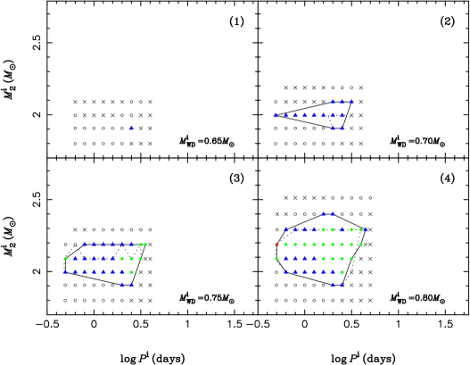
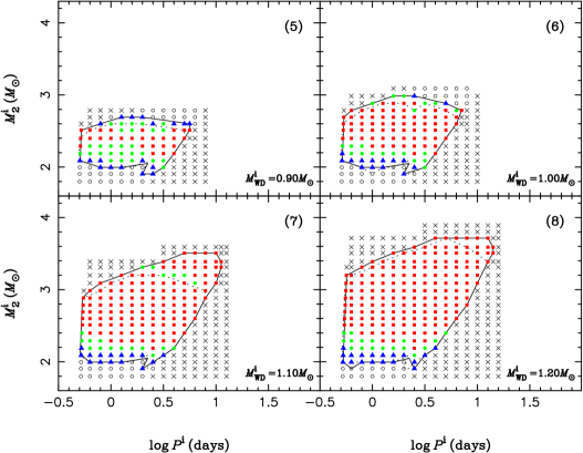
Figure 7: Final outcomes of the binary evolution calculations in the CEW model in the initial orbital period – secondary mass ($\log P^{\rm i},M_{\rm 2}^{\rm i}$) plane, where $P^{\rm i}$ is the initial orbital period, and $M_{\rm 2}^{\rm i}$ is the initial mass of the donor star (for different initial WD masses as indicated in each panel). Filled squares indicate SN Ia explosions during a CE phase ($M_{\rm CE}>0$). Filled circles denote that SN Ia explosions occur in the SSS phase ($\dot{M}_{\rm cr}\geq|\dot{M}_{\rm 2}|\geq\frac{1}{2}\dot{M}_{\rm cr}$ and $M_{\rm CE}=0$), while filled triangles denote that SN Ia explosions occur in the RN phase ($\frac{1}{2}\dot{M}_{\rm cr}>|\dot{M}_{\rm 2}|\geq\frac{1}{8}\dot{M}_{\rm cr}$ and $M_{\rm CE}=0$). Open circles indicate systems that experience nova explosions, preventing the CO WD from reaching 1.378 $M_{\odot}$ ($|\dot{M}_{\rm 2}|<\frac{1}{8}\dot{M}_{\rm cr}$ and $M_{\rm CE}=0$), while crosses show the systems that are unstable to dynamical mass transfer. The solid curves show the contours of the parameter space leading to SNe Ia for the CEW model, while, for comparison, the dotted curves show the contours from the OTW model (taken from Meng et al. 2009a).

3.2 Final outcomes of the binary evolution calculations

To clearly show the difference between our results and previous ones in literatures, we show the final outcomes of all the binary evolution calculations in an initial orbital period – secondary mass ($\log P^{\rm i},M_{\rm 2}^{\rm i}$) plane (Fig. 7). As the figure shows, CO WDs may reach a mass of 1.378 $M_{\odot}$ while the system is still in the CE phase (filled squares) or after the CE evolution has ended, where they can be either in stable (filled circles) or weakly unstable (filled triangles) hydrogen-burning phases. Systems re-emerging from the CE phase may show the properties of SSSs if hydrogen burning on the WD is stable or those of RNe for weakly unstable hydrogen burning. All these systems are probably progenitors of SNe Ia. Because of dynamically unstable mass transfer or strong hydrogen shell flashes, many CO WDs do not increase their masses to 1.378 $M_{\odot}$. As shown in Figs. 4 and 5, in comparison to the OTW model, the longer timescale for the CEW phase and the higher mass-growth rate during this phase result in a larger increase of the CO WD mass in this phase. Consequently the timescale from the end of the CEW to the explosion (where the systems may appear as SSSs or RNe) is shorter, or the CO WD, which would not increase to 1.378 $M_{\odot}$ in the OTW phase, may reach 1.378 $M_{\odot}$ during the CEW phase (the system then will not appear as a SSS or RN system). This means that a given system is less likely to be in the SSS/RN phase at the SN explosion in the CEW model (Meng et al. 2009a, c). Based on the supersoft X-ray flux in elliptical galaxies, Gilfanov & Bogdán (2010) concluded that no more than 5% of SNe Ia in early-type galaxies can be produced by mass-accreting white dwarfs from the SD scenario. According to the OTW model, Meng & Yang (2011b) found that the mean relative duration of the SSS phase for an accreting WD is about 5%. However, based on the small number of SSSs observed in some galaxies such as M31, Maoz, Mannucci & Nelemans (2014) argued that no more than 1 % of the WD’s growth time is spent in the SSS phase. This is an order of magnitude less than was found by Meng & Yang (2011b). The results here should help to resolve the conflict between Maoz, Mannucci & Nelemans (2014) and Meng & Yang (2011b) since the CE phase in the CEW model lasts longer than the OTW phase. Moreover, even if the binary system were in a SSS phase, the supersoft X-ray flux would also be strongly reduced by the CSM that forms because of the CEW or the OTW, but the CSM from our CEW model would be more efficient in suppressing the supersoft X-ray flux because of the relatively high CSM density due to the much lower wind velocity (Nielsen et al. 2013; Wheeler & Pooley 2013).

In Fig. 7 we present contours of the initial parameters leading to SNe Ia for different WD masses, indicating the final state of the system, while Fig. 8 combines the contours in one summary plot. The left boundaries of the contours are determined by the radii of ZAMS stars, i.e. correspond to systems that start RLOF on the ZAMS; systems beyond the right boundaries experience dynamically unstable mass transfer at the base of the red-giant branch (RGB). The upper boundaries are determined by systems that experience a delayed dynamical instability. For the systems above the lower boundaries, the mass-transfer rate is larger than $\frac{1}{8}\dot{M}_{\rm cr}$, which prevents the occurrence of strong hydrogen shell flashes, while, at the same time, the secondaries can provide enough material to feed the growth of the CO WDs to allow it to reach 1.378 $M_{\odot}$. The figure shows that the initial WD mass significantly affects the upper boundary but not the lower boundary. The upper boundary moves to lower masses as the initial WD mass decreases, causing a shrinking of the initial parameter space that leads to SNe Ia with a decrease of the WD mass; at $M_{\rm WD}^{\rm i}=0.65\,M_{\odot}$ the contour collapses to a point.

3.3 Comparison with the OTW model

Fig. 7 also shows the contours of initial parameters leading to SNe Ia from the OTW model for comparing the two model. The shapes of the contours are quite similar to each other, except that the upper boundary of the CEW model is higher than that in the OTW model and that the maximum initial orbital period for the CEW model can be longer; this means that mass transfer between the binary components is somewhat more stable for the CEW model than for the OTW model. This phenomenon is mainly caused by the different treatment of the mass-growth rate of the CO WD; i.e. the mass-growth rate during the CE evolution phase in the CEW model is higher than that during the OTW phase in the OTW model. So, for a given binary system, the WD mass (the mass ratio, $M_{\rm 2}/M_{\rm WD}$) at the same evolutionary stage for the CEW model is slightly higher (smaller) than in the OTW model, which leads to relatively more stable mass transfer for the CEW model. Especially in the right-upper part of the allowed parameter space for the CEW model, the systems will experience nova explosions, preventing the CO WD from reaching 1.378 $M_{\odot}$ for the OTW model, while the WD will reach 1.378 $M_{\odot}$ in the CE phase for the CEW model. This difference arises from the fact that the CE acts as a mass reservoir which can continuously feed material to the WD as long as the CE exists, even when $|\dot{M}_{\rm 2}|<\dot{M}_{\rm cr}$ as shown in Fig. 4.

Another difference is the minimum initial mass of CO WDs, $M_{\rm WD}^{\rm min}$, that can lead to SNe Ia. Previous studies showed that the minimum initial mass may be as low as $0.67\,M_{\odot}$ for $Z=0.02$ based on the OTW model (Langer et al. 2000; Han & Podsiadlowski 2004), and Meng et al. (2009a) found that $M_{\rm WD}^{\rm min}$ strongly depends on metallicity. Here, the minimum mass of CO WDs for $Z=0.02$ is $0.65\,M_{\odot}$, slightly lower than that for the OTW model, which is also a direct consequence of the different treatment of the mass-growth rate of the WDs.

These differences between the CEW model and the OTW model already indicate that the birth rate of SNe Ia in the CEW model should be somewhat higher than in the OTW model (see section 5).

3.4 The final state of the systems

In this section, we examine the final state of the binary systems and the properties of the companions at the time of the supernova explosion (assumed to occur when the WD mass has reached $M_{\rm WD}=1.378\,M_{\odot}$); this may be helpful for identifying SN Ia progenitor systems or for finding surviving companions in supernova remnants.

Figure 8: The contours of initial parameters in the ($\log P^{\rm i},M_{\rm 2}^{\rm i}$) plane for different initial WD masses for which SNe Ia are expected. For $M_{\rm WD}^{\rm i}=0.65\,M_{\odot}$, the contour shrinks to a point and is not included in the figure.

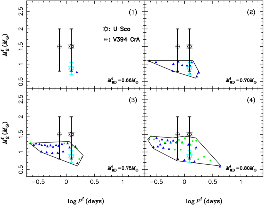
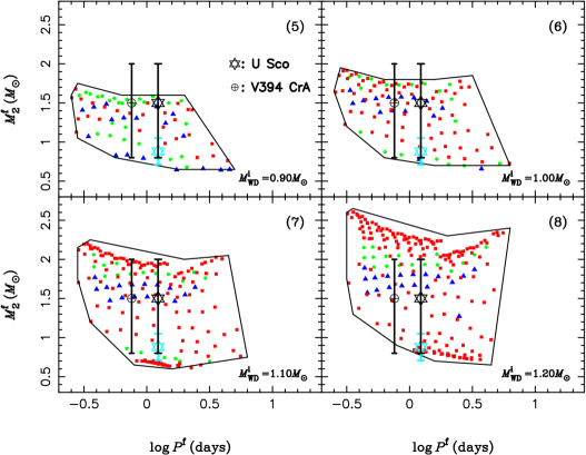
Figure 9: Similar to Fig. 7 but for the final state of the binary systems in the CEW model in the final orbital period – secondary mass ($\log P^{\rm f},M_{\rm 2}^{\rm f}$) plane, where $P^{\rm f}$ is the final orbital period, and $M_{\rm 2}^{\rm f}$ is the final mass of the donor star (for different initial WD masses as indicated in each panel) at the moment of $M_{\rm WD}=1.378~{}M_{\odot}$. Filled squares indicate SN Ia explosions during a CE phase ($M_{\rm CE}>0$). Filled circles denote that SN Ia explosions occur in the SSS phase ($\dot{M}_{\rm cr}\geq|\dot{M}_{\rm 2}|\geq\frac{1}{2}\dot{M}_{\rm cr}$ and $M_{\rm CE}=0$), while filled triangles indicate that SN Ia explosions occur in the RN phase ($\frac{1}{2}\dot{M}_{\rm cr}>|\dot{M}_{\rm 2}|\geq\frac{1}{8}\dot{M}_{\rm cr}$ and $M_{\rm CE}=0$). The solid curves show the contours of the parameter space. Two recurrent novae are indicated by a hexagram for U Sco and an Earth symbol for V394 CrA, where the position of the black hexagram is based on the the model simulation by Hachisu et al. (2000a, b), while the bright blue hexagram taken from the dynamical estimate (Thoroughgood et al. 2001).

3.4.1 Final contour

Fig. 9 shows the final states of binary systems leading to SNe Ia in the ($\log P^{\rm f}-M_{\rm 2}^{\rm f}$) plane when $M_{\rm WD}=1.378~{}M_{\odot}$ for different initial WD masses, while Fig. 10 compares the initial and final contours of these systems. Generally, for a system with given initial parameters, the companion is still massive enough to maintain a high mass-transfer rate at the moment when $M_{\rm WD}=1.378~{}M_{\odot}$. For example, many systems are still in the CEW phase at this moment; this means that the WDs in these systems would continue to increase their masses if the WDs did not explode at this stage. Even for the systems exploding in the SSS or RN phase, the companions may still be massive enough to maintain a high mass-transfer rate, so that the WDs could continue to grow in mass if they did not explode when $M_{\rm WD}=1.378~{}M_{\odot}$ (see Figs. 2 and 9). In other words, if the WD of a system is slightly less massive than 1.378 $M_{\odot}$ and its companion mass and orbital period are also located in the final contours for SNe Ia, it is still very likely for the WD to continue to increase its mass to 1.378 $M_{\odot}$. Fig. 10 shows that the positions of the final contours are below those of the initial contours; the secondary always has a mass less than 2.6 $M_{\odot}$, but can be as low as $0.6\,M_{\odot}$. Almost all models have a final orbital period between 0.22 d and 6.5 d; these periods are generally shorter than in the OTW model (see Meng et al. 2009c). Similar to the initial contours, the parameter range of the final contours shrinks with decreasing initial WD mass and disappears when $M_{\rm WD}=0.65\,M_{\odot}$. A SSS (RX J0513.9-6951) and three RNe (CI Aql, U Sco and V394 CrA) are also indicated in Fig. 10 and two RNe (U Sco and V394 CrA) in Fig. 9. These objects have been considered good candidates for progenitor systems of SNe Ia as they contain massive WDs and have short orbital periods (Parthasarathy et al. 2007). Numerical simulations provide further support for the SN Ia progenitor connection (see below). RX J0513.9-6951 (open star) with $M_{\rm WD}=1.30\,M_{\odot}$ (Hachisu & Kato 2003b) is located within the initial contour for SN Ia progenitors. If the WD is a CO WD, it would make an excellent candidate for a SN Ia progenitor, as already suggested in Hachisu & Kato (2001) and Hachisu & Kato (2003b). For CI Aql, Sahman et al. (2013) recently analyzed time-resolved, intermediate-resolution spectra during quiescence and found a WD mass of $1.00\pm 0.14\,M_{\odot}$ and a secondary mass of $2.32\pm 0.19\,M_{\odot}$. The position of CI Aql is also perfectly placed within the initial contours for SNe Ia. Even considering the uncertainty in the WD mass, our model suggests that CI Aql is another excellent SN Ia progenitor candidate system.

The dynamical mass estimates for the binary components in U Sco are $M_{\rm WD}=1.55\pm 0.24\,M_{\odot}$ and $M_{\rm 2}=0.88\pm 0.17\,M_{\odot}$ (Thoroughgood et al. 2001), while model simulations show U Sco to be a WD + MS system with $M_{\rm WD}=1.37\,M_{\odot}$ and $M_{\rm 2}=1.5\,M_{\odot}$, although a mass between $0.8\,M_{\odot}$ and $2.0\,M_{\odot}$ is also acceptable (Hachisu et al. 2000a, b, see also the binary evolution model in Podsiadlowski 2003). Both the dynamical estimates and model simulations indicate that the mass of the WD in U Sco is quite close to 1.378 $M_{\odot}$. Figs. 9 and 10 that show that U Sco is well located within the final contours for SNe Ia, irrespective of whether the companion mass is taken from model simulations or dynamical estimates; this suggests that the companion has enough material to maintain a high mass-transfer rate to increase the WD mass to 1.378 $M_{\odot}$. Therefore, our model supports the previous suggestion that, if the WD in U Sco is a CO WD, it is an excellent candidate for a SN Ia progenitor. However, whether or not the massive WD is a CO or a ONeMg one is still under debate (Mason 2011; Kato & Hachisu 2012). Further effort, both on the observational and the theoretical side, is clearly needed to decide the fate of U Sco. The WD mass of V394 CrA has been estimated to be 1.37 $M_{\odot}$, while the mass of the companion is still unclear. The best-fit companion mass for this recurrent nova system is 1.50 $M_{\odot}$, while a mass between $0.8\,M_{\odot}$ and $2.0\,M_{\odot}$ is still acceptable (Hachisu & Kato 2000, 2003a; Hachisu et al. 2003). In either case, it is still very likely that the WD can increase its mass to 1.378 $M_{\odot}$. Assuming a CO composition for the WD of V394 CrA, our results confirm that it provides an excellent candidate for a SN Ia progenitor. In any case, further observations are necessary to determine the masses of the WD and the secondary in V394 CrA.

In addition, as the well candidates of the progenitors of SNe Ia, U Sco and V394 CrA provide an opportunity to examine the progenitor models of SNe Ia in a detailed way, i.e. whether or not the two RNe may locate in the RN region for SNe Ia predicted by any successful single-degenerate model. In Fig. 9, although the expected regions for the CEW, SSS and phases overlapped each other, the RN region predicted by our CEW model may explain the positions of U Sco and V394 CrA in the ($\log P^{\rm f}-M_{\rm 2}^{\rm f}$) plane. According to Fig. 9, both U Sco and V394 CrA are likely to come from systems with an initial WD mass between $1.0~{}M_{\odot}$ and $1.1~{}M_{\odot}$ if the best-fit companion masses from model simulations are taken, while the dynamical estimate for U Sco favors a system with $M_{\rm WD}^{\rm i}\leq 0.9~{}M_{\odot}$.

3.4.2 Mass and orbital velocity

In Fig. 11 we show the parameter regions for the companion mass and its orbital velocity when $M_{\rm WD}=1.378\,M_{\odot}$ for different initial WD masses. The ranges of companion mass and orbital velocity here are very similar to those shown in Han (2008) and Meng & Yang (2010b) although their results were based on the OTW model. At the time of the supernova, the companion mass lies between 0.6 $M_{\odot}$ and 2.6 $M_{\odot}$ and the orbital velocity between 60 ${\rm km\,s^{\rm-1}}$ and 260 ${\rm km\,s^{\rm-1}}$. The impact of the supernova ejecta with the envelope of the companion may strip off some hydrogen-rich material from the surface of the companion. At the same time, the companion may receive a velocity kick, i.e. the final space velocity of a surviving companion in a supernova remnant is $v_{\rm s}=\sqrt{v_{\rm orb}^{\rm 2}+v_{\rm kick}^{\rm 2}}$ (Marietta et al. 2000; Meng et al. 2007; Pakmor et al. 2008; Liu et al. 2012). Generally, the stripped-off material is much less massive than the companion, and the kick velocity is much smaller than the orbital velocity. In any case, the companion mass and its orbital velocity here should be taken as upper and lower limits for the mass and the space velocity of the surviving companion in a supernova remnant, respectively. In the figure, we also plotted the parameters for the potential surviving companion of Tycho’s supernova (Tycho G, Ruiz-Lapuente et al. 2004; González-Hernández et al. 2009; Bedin et al. 2014). Although it is presently unclear whether Tycho G actually is the surviving companion (see the discussion in section 3.4.3), its claimed parameters would be compatible with the range of the companion mass and its orbital velocity presented here.

Figure 10: Parameter regions producing SNe Ia in the ($\log P-M_{\rm 2}$) plane for WD + MS systems with different initial WD masses in the CEW model. In the WD + MS systems inside the region enclosed by the red curves (labelled “initial”), the white dwarf is able to grow to a mass of 1.378 $M_{\odot}$, where a SN Ia explosion is assumed to occur. The final state of the WD + MS systems is enclosed by the black curves (labelled “final”). A supersoft X-ray source, RX J0513.9-6951 (open star) is also plotted; its orbital period is 0.763 d (Pakull et al. 1993). Three recurrent novae are indicated by a hexagram for U Sco (with a period of 1.2306 d; Schaefer & Ringwald 1995; Hachisu et al. 2000a, b), a solar symbol for CI Aql (with an orbital period of 0.6184 d; Mennickent & Honeycut 1995; Sahman et al. 2013) and an Earth symbol for V394 CrA (with an orbital period of 0.7577 d; Schaefer 1990), where the black hexagram assumes the companion mass from the model simulation by Hachisu et al. (2000a, b), while the red hexagram takes it from the dynamical estimate (Thoroughgood et al. 2001).

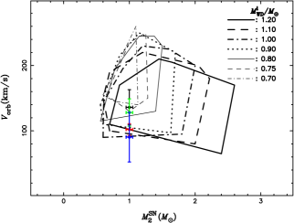
Figure 11: Parameter space for the companion mass and its orbital velocity when $M_{\rm WD}=1.378\,M_{\odot}$ for different initial WD masses in the CEW model. The cross represents the potential companion of Tycho’s supernova progenitor, Tycho G, and the length of the cross indicates the typical observational errors, where the space velocities for Tycho G are taken from Ruiz-Lapuente et al. (2004) (black), González-Hernández et al. (2009) (green), Kerzendorf et al. (2009) (blue) and Bedin et al. (2014) (red).

Figure 12: Parameter regions for the companion radius and its equatorial rotational velocity when $M_{\rm WD}=1.378\,M_{\odot}$ for different initial WD masses in the CEW model.

3.4.3 Companion radius and rotational velocity

In Fig. 12, we present the parameter regions for the companion radius and its equatorial rotational velocity when $M_{\rm WD}=1.378\,M_{\odot}$ for different initial WD masses. In our calculations, we did not keeptrack of the companion radius as it can be obtained by some simple assumptions. We assume that the companion radius is equal to its Roche-lobe radius, i.e. the companion is filling its Roche lobe at the moment of the supernova explosion, and the donor’s radius will not be far away from that shown in Fig. 12. The equatorial rotation velocity is calculated assuming that the companion star co-rotates with the orbit. The figure shows that the rotational velocity of the surviving companions ranges from 40 km s^-1 to 220 km s^-1; this means that, in many cases, the companions’ spectral lines should be noticeably broadened if the rotation of the star is not affected by the impact of the supernova ejecta. We note that the upper limit of the rotational velocity here is higher than that based on the OTW model in Han (2008) (170 km s^-1) since the final orbital periods tend to be shorter in the CEW model than in the OTW model (see Figs. 2 and 3). The companion radius lies between 0.5 $R_{\odot}$ and 9 $R_{\odot}$. In general, the companion stars with larger radii have lower rotational velocities. This figure may be helpful for identifying the companion nature of a potential surviving candidate in a supernova remnant. However, although the radius of Tycho G ($1-3\,R_{\odot}$) matches well with our calculations, its rotational velocity is much smaller than predicted here; this is the reason why Kerzendorf et al. (2009) have strongly argued against Tycho G being the surviving companion of Tycho’s supernova. Here, we do not consider the impact of the supernova ejecta on the companion. If the companion expands significantly because of the impact, its rotational velocity will be significantly reduced. Indeed, as argued by Kerzendorf et al. (2009) (also see Meng & Yang 2011a), it is possible in principle to explain the observed rotational velocity in Tycho G if the companion’s envelope was almost completely stripped by the supernova impact and the surface layers we see now had to expand from regions near the core. These expectations, that follow from simple angular-momentum conservation considerations, have been confirmed by numerical simulations (e.g. Pan et al. 2012a; Liu et al. 2013), though we note that none of the simulations in Pan et al. (2012a) can explain the observed properties of Tycho G as none can fit the observed gravity ($\log g$) and the observed rotational velocity simultaneously.

Figure 13: The parameter regions for the luminosity and the temperature of the companion when $M_{\rm WD}=1.378\,M_{\odot}$ for different initial WD masses. The star represents the potential surviving companion star of Tycho’s supernova, Tycho G, where the bar represents the observational error (Ruiz-Lapuente et al. 2004).

3.4.4 Luminosity and effective temperature

Fig. 13 shows the parameter regions for the luminosity and the temperature of the companion when $M_{\rm WD}=1.378\,M_{\odot}$ for different initial WD masses. The luminosity ranges from $0.25\,L_{\odot}$ to $100\,L_{\odot}$, and the effective temperature from $4470$ K to $12600$ K. The range of effective temperatures is slightly larger than in the OTW model (Han 2008), which again is a direct consequence of the different treatment of the mass-growth rate of the WD, leading to a larger initial parameter space in the initial secondary mass – orbital period plane.

The luminosity and the effective temperature of a companion will generally be affected by the impact of the supernova ejecta (Marietta et al. 2000; Podsiadlowski 2003; Shappee et al. 2013); hence Fig. 13 can only give an indication for the initial conditions when exploring the evolution and appearance of a companion star during the post-impact re-equilibration phase when the star is out of thermal equilibrium. Podsiadlowski (2003) calculated the luminosity evolution of a subgiant star of 1 $M_{\odot}$ after being hit by the ejecta of a SN Ia and found that the luminosity evolution was initially much faster than the Kelvin-Helmholtz timescale of the pre-SN subgiant since the re-equilibration timescale is determined by the thermal timescale of the outer layer of the star, which can be many orders of the magnitude shorter. Depending on the amount of energy deposited, the luminosity of the companion may be either significantly overluminous or underluminous ($0.1\,L_{\odot}$ – $200\,L_{\odot}$) 440 yr after the SN explosion. Pan et al. (2012b) found that the evolution of the remnant star strongly depends not only on the amount of energy deposited from the explosion but also on the depth of the energy deposition and that the luminosity of the remnant could be close to that of Tycho G $\sim 500$ yr after the explosion (consistent with the conclusions of Podsiadlowski 2003). Shappee et al. (2013) calculated the future evolution of the companion by injecting $(2-6)\times 10^{\rm 47}$ erg of energy into the stellar-evolution model of a 1 $M_{\odot}$ donor star and found that the companion becomes significantly more luminous ($10-10^{\rm 3}\,L_{\odot}$) for a long period of time ($10^{\rm 3}-10^{\rm 4}$ yr) due to the Kelvin-Helmholtz collapse of the envelope. These simulations and our binary evolution calculations partly share the luminosity range, especially for the results in Podsiadlowski (2003). The potential surviving companion of Tycho’s supernova is well located within the contour of Fig. 13. However, as we discussed in section 3.4.3, no model to date can reproduce $\log g$, the rotation velocity and the luminosity of Tycho G simultaneously. Observations are also not fully conclusive. While Bedin et al. (2014) in their re-analysis conclude that the proper motion and chemical abundance of Tycho G are consistent with it being a surviving companion, Xue & Schaefer (2015), measuring the exact explosion site of Tycho’s supernova, found that Tycho G is outside the 1$\sigma$ error region (7.3 arcsec) at very high significance. Therefore Tycho G may just be a Milky Way thick-disc star that happens to pass in the vicinity of the supernova remnant (Fuhrmann 2005; but also see Bedin et al. 2014 for a different view).

Figure 14: The parameter regions for the mass-lose rate and the total amount of material lost from the system when $M_{\rm WD}=1.378\,M_{\odot}$ for different initial WD masses, where the CE mass is included in the amount of material lost from the system.

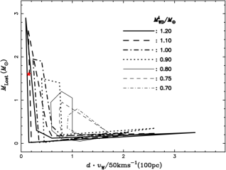
Figure 15: The parameter regions for the total amount of material lost from the system and the maximum distance that the lost material may reach by the time when $M_{\rm WD}=1.378\,M_{\odot}$ for different initial WD masses; here the CE mass is included in the amount of material lost from the system. The red star represents the Galactic SN remnant RCW 86 (Broersen et al. 2014).

3.4.5 Mass loss

Fig. 14 shows the mass-lose rate from the system and the total amount of material lost when $M_{\rm WD}=1.378\,M_{\odot}$. Here, the CE mass is included in the material lost since the CE material may generally be lost eventually (see the further discussion in section 6.1) or provide a mass reservoir to form a circumbinary disk. This assumption for the material lost is reasonable for about 99% of all SNe Ia, because the CE mass is so small (less massive than $\sim 10^{\rm-3}~{}M_{\odot}$) for most SNe Ia exploding in the CE phase. Only for the cases of $M_{\rm WD}^{\rm i}\geq 1.1~{}M_{\odot}$, may this assumption affect the upper parts of the contours, i.e. the upper limit of the amount of the lost material may be overestimated by a few tenths $M_{\odot}$ if one assumes that the CE contributes to the lost material. As Fig. 14 shows, the mass-lose rate covers 3 orders of magnitude, i.e. from $\sim 10^{\rm-8}\,M_{\odot}\,{\rm yr}^{\rm-1}$ to $10^{\rm-5}\,M_{\odot}\,{\rm yr}^{\rm-1}$. The lower limit of the mass-loss rate for the CEW model is mainly constrained by the mass loss during helium shell burning, while the upper limit is mainly determined by the Eddington luminosity. The lower mass-loss rate from systems in the CEW model may help to explain why the circumstellar environment contains very little mass around some SNe Ia such as SN 2011fe (Patat et al. 2013), although there are ongoing arguments on whether SN 2011fe originates from a SD or a DD system (Li et al. 2011b; Chomiuk 2013; Mazzali et al. 2014; Meng & Han 2016).

In our model, a large amount of material may be lost from the CE surface: it may be as large as $2.5\,M_{\odot}$. This could be the cause of the colour excess seen in SNe Ia (Meng et al. 2009b). As this material cools, part of it may form dust and cause light echoes (Wang et al. 2008; Yang et al. 2015). The dust should be distributed over a large region around SNe Ia, where the extent should be smaller than the maximum distance that the lost material can reach. Fig.  15 shows the contour of the total amount of material lost from the system and the maximum distance that the lost material may reach by the time when $M_{\rm WD}=1.378\,M_{\odot}$. The maximum distance is simply $d=v_{\rm w}\times t_{\rm d}$, where $v_{\rm w}$ is the wind velocity of the material lost, here assumed to be 50 ${\rm km}$ ${\rm s}^{\rm-1}$, and $t_{\rm d}$ is the delay time from the onset of mass transfer to the moment when $M_{\rm WD}=1.378\,M_{\odot}$. There is a trend in Fig.  15 that the maximum distance is closer if a larger amount of material is lost. This is caused by the effect of the initial WDs and the companions on the mass-transfer time scale: for a lower initial WD mass and a lower companion mass, the mass-transfer timescale for increasing the WD to 1.378 $M_{\odot}$ is longer, and the wind material can reach a larger distance. At the same time, a less massive companion means a lower mass-transfer rate and consequently much lower mass-loss rate, which results in a smaller amount of the lost material although the mass-transfer timescale is longer. In particular, for some SNe Ia, the amount of lost material is quite small (no more than 0.2 $M_{\odot}$), but is spread over a very large scale ($\sim 300$ pc). In these cases, the environment around the SNe Ia should be very clean. In a follow-up paper, we will discuss the observational consequences of these properties in a detailed binary population synthesis study.

We must emphasize that the results from Fig. 10 to Fig. 15 are based on the assumption that the WD explodes as a SN Ia when its mass reaches 1.378 $M_{\odot}$. However, the explosion could be delayed if the WD is rotating rapidly (see the discussion in section 5.2), in which case the final state of the binary system could be quite different from what is presented here. For example, the range of the companion mass should move to a lower value and the range of the final orbital period may be increased, i.e. range from a value lower than 0.2 d to one longer than 6.5 d. Similarly, the range of the radius, rotation velocity and orbital velocity are also increased, i.e. the lower boundary moves to a lower value while the upper boundary moves to a higher value. As a consequence, $M_{\rm lost}$ would be larger, while the final mass-loss rate from the binary system would be lower, producing a cleaner environment around the SN Ia.

4 Binary population synthesis

Adopting the results in section 3, we have estimated the expected supernova frequency from the WD+MS channel using the rapid binary evolution code developed by Hurley et al. (2000, 2002). Hereafter, we use primordial to refer to the binaries before the formation of the WD+MS systems and initial for the WD+MS systems (see also Meng et al. 2009a and Meng & Yang 2010a).

4.1 Common-envelope evolution

In the evolution of a binary, the primordial mass ratio (the ratio of the mass of the primary to the mass of the secondary) is crucial for the nature of the first mass-transfer phase. There is a critical mass ratio, $q_{\rm c}$, which determines the evolutionary direction of a binary system. If the primordial mass ratio is larger than $q_{\rm c}$, the system will experience dynamically unstable mass transfer and the system will enter into a CE phase (Paczyński 1976). The value of $q_{\rm c}$ is a function of the evolutionary state of the primordial primary at the onset of RLOF (Hjellming & Webbink 1987; Webbink 1988; Han et al. 2002; Podsiadlowski et al. 2002; Chen & Han 2008). In this paper, we set $q_{\rm c}$ = 4.0 if the primary fills its Roche lobe on the MS or in the HG. Such a value is supported by various detailed binary evolution studies (Han et al. 2000; Chen & Han 2002, 2003). If the primordial primary fills its Roche lobe on the first giant branch (FGB) or AGB, we adopt

$$q_{\rm c}=\left[1.67-x+2\left(\frac{M_{\rm c1}^{\rm P}}{M_{\rm 1}^{\rm P}}\right)^{\rm 5}\right]/2.13,$$ (18)

where $M_{\rm c1}^{\rm P}$ is the core mass of the primordial primary, and $x={\rm d}\ln R_{\rm 1}^{\rm P}/{\rm d}\ln M_{\rm 1}^{\rm p}$ is the mass-radius exponent of the primordial primary, where $x\simeq 0.3$ and changes with the stellar composition. If the mass donors (primaries) are naked helium giants, we take $q_{\rm c}$ = 0.748 (see details in Hurley et al. 2002).

The “new” binary embedded in the CE consists of the dense core of the primordial primary and the primordial secondary and will lose its orbital energy due to the friction between the CE and the binary system. A part of the orbital energy released by the system during the spiral-in process is injected into the envelope to eject the material in the CE (Livio & Soker 1988). In this paper, we assume that the CE is ejected completely if

$$\alpha_{\rm CE}\Delta E_{\rm orb}=|E_{\rm bind}|,$$ (19)

where $E_{\rm bind}$ is the binding energy of the CE, $\Delta E_{\rm orb}$ is the orbital energy released during the spiral-in phase, and $\alpha_{\rm CE}$ denotes the CE ejection efficiency (i.e. the fraction of the released orbital energy that can be used in ejecting the CE). Since the internal energy and, in particular, the recombination energy in the envelope is not incorporated in the binding energy (Ivanova et al. 2013, 2015), $\alpha_{\rm CE}$ can be larger than 1 (see Han, Podsiadlowski & Eggleton 1995 on the discussion of the internal energy). Here, $\alpha_{\rm CE}=1.0$ or $\alpha_{\rm CE}=3.0$ is adopted.

4.2 Evolutionary channels for WD + MS systems

There are three evolutionary channels to form WD + MS systems based on the evolutionary state of the primordial primary at the onset of the first RLOF.

Case 1 (He star channel): the primordial primary is in the HG or on the RGB at the onset of the first RLOF phase (so-called case B evolution as defined by Kippenhahn & Weigert 1967). In this case, a CE forms either because of a large mass ratio or because the mass donor has a deep convective envelope. After CE ejection, the system consists of a helium star and a MS star. The helium star continues to evolve and will fill its Roche lobe again after helium has been exhausted in the center. Due to the small mass ratio, mass transfer is dynamically stable leading to the formation a close CO WD + MS system (see Nomoto et al. 1999, 2003 for details).

Case 2 (EAGB channel): the primordial primary is on the early AGB stage (EAGB) (i.e. helium is exhausted in the core, while thermal pulses have not yet started). At this stage, the hydrogen-exhausted core, i.e. the CO core surrounded by a dense helium shell, is much denser than the hydrogen-rich envelope, and there is a steep gradient in the gravitational potential between the hydrogen-exhausted core and the hydrogen-rich envelope (e.g. Figure. 2 in Meng et al. 2008). If the system experiences dynamically unstable mass transfer, the system will enter a CE and spiral-in phase where the hydrogen-rich envelope forms a CE. After the ejection of the CE, the new, much closer binary consists of the hydrogen-exhausted core and the secondary. Eventually the primordial primary becomes a helium red giant and may fill its Roche lobe to start a second phase of RLOF. Similarly to the He star channel, this RLOF phase is stable and produces WD + MS systems after the end of RLOF.

Case 3 (TPAGB channel): the primordial primary fills its Roche lobe during the TPAGB stage. Similarly to the above two channels, a CE is formed during the first RLOF phase. A CO WD + MS binary is produced after CE ejection.

The WD + MS systems continue to evolve, and the MS companions will, at some stage, fill their Roche lobes and transfer matter to the CO WDs, which may subsequently explode as SNe Ia. Here, we assume that, if the initial orbital period, $P_{\rm orb}^{\rm i}$, and the initial secondary mass, $M_{\rm 2}^{\rm i}$, of a WD + MS system are located in the appropriate region in the ($\log P^{\rm i},M_{\rm 2}^{\rm i}$) plane (see Fig. 7) for SNe Ia at the onset of RLOF, a SN Ia is produced.

4.3 Basic parameters for the Monte-Carlo simulations

To investigate the birth rate of SNe Ia, we followed the evolution of $10^{\rm 7}$ binaries using the Hurley rapid binary evolution code (Hurley et al. 2000, 2002). The results of the grid calculations in section 3 are incorporated into the code. The primordial binary samples are generated in a Monte-Carlo way, where circular orbits are assumed for all binaries. The basic parameters for the simulations are as follows:

(i) The initial mass function (IFM) of Miller & Scalo (1979) is adopted. The primordial primary is generated according to the formula of Eggleton et al. (1989)

$$M_{\rm 1}^{\rm p}=\frac{0.19X}{(1-X)^{\rm 0.75}+0.032(1-X)^{\rm 0.25}},$$ (20)

where $X$ is a random number in the range [0,1], and $M_{\rm 1}^{\rm p}$ is the mass of the primordial primary, which is between 0.1 $M_{\rm\odot}$ and 100 $M_{\rm\odot}$.

(ii) For the evolution of a binary system, the primordial mass ratio, $q^{\prime}$, is a crucial parameter as it determines the evolutionary direction of the system. In the paper, a uniform mass-ratio distribution is adopted, i.e $q^{\prime}$ is uniformly distributed in the range $[0,1]$ (Mazeh et al. 1992; Goldberg & Mazeh 1994):

$$n(q^{\prime})=1,\hskip 56.9055pt0<q^{\prime}\leq 1,$$ (21)

where $q^{\prime}=M_{\rm 2}^{\rm p}/M_{\rm 1}^{\rm p}$.

(iii) All stars are assumed to be members of binary systems. For the separation of the binary systems, a constant distribution in $\log a$ is assumed for wide binaries, while $a$ falls off smoothly for close binaries:

$$a\cdot n(a)=\left\{\begin{array}[]{lc}\alpha_{\rm sep}(a/a_{\rm 0})^{\rm m}&a\leq a_{\rm 0};\\ \alpha_{\rm sep},&a_{\rm 0}<a<a_{\rm 1},\\ \end{array}\right.$$ (22)

where $\alpha_{\rm sep}\approx 0.070$, $a_{\rm 0}=10\,R_{\odot}$, $a_{\rm 1}=5.75\times 10^{\rm 6}\,R_{\odot}=0.13\,{\rm pc}$ and $m\approx 1.2$. The separation distribution adopted here implies an equal number of wide binary systems per logarithmic interval, and gives approximately 50 percent of binary systems with an orbital period $\leq 100$ yr (see also Han, Podsiadlowski & Eggleton 1995).

(iv) We simply adopt either a single starburst (i.e. $10^{\rm 11}\,M_{\odot}$ in stars is generated at a single instant of time) or a constant star-formation rate $S$ (SFR) for the last 15 Gyr. Here the value of $S$ is set to be $5\,M_{\odot}\,{\rm yr^{-1}}$, which is calibrated to maintain the production of one binary with $M_{\rm 1}>0.8\,M_{\odot}$ in the Galaxy every year (see Iben & Tutukov 1984; Han, Podsiadlowski & Eggleton 1995; Hurley et al. 2002; Willems & Kolb 2004). The value of $5\,M_{\odot}\,{\rm yr^{-1}}$ can successfully reproduce the birth rate of the core-collapse supernova and the ²⁶Al 1.809-MeV gamma-ray line in the galaxy (Timmes et al. 1997).

5 Binary population synthesis results

Figure 16: The evolution of the birth rates of SNe Ia for a constant star formation rate (Z=0.02, SFR=$5\,M_{\rm\odot}\,{\rm yr^{\rm-1}}$). The solid and dashed curves show the cases with $\alpha_{\rm CE}=1.0$ and $\alpha_{\rm CE}=3.0$, respectively.

Figure 17: The evolution of the birth rates of SNe Ia for a single starburst of $10^{\rm 11}\,M_{\odot}$. The solid and dashed curves show the cases with $\alpha_{\rm CE}=1.0$ and $\alpha_{\rm CE}=3.0$, respectively.

5.1 The birth rate

Fig. 16 shows the Galactic birth rates of SNe Ia (i.e. $Z=0.02$ and SFR= 5.0 $M_{\odot}\,{\rm yr}^{\rm-1}$) from the WD+MS channel. The Galactic birth rate is around (0.89-1.20)$\times 10^{\rm-3}\,{\rm yr^{\rm-1}}$, which is higher than that from the OTW model by about $\sim 30\%$ (see Fig. 6 in Meng et al. 2009a), as one would expect since the parameter space for SNe Ia here is larger in our model than in the OTW model. This result is somewhat lower but still comparable to that inferred from observations (3-7$\times 10^{\rm-3}\,{\rm yr^{\rm-1}}$, van den Bergh & Tammann 1991; Cappellaro & Turatto 1997; Li et al. 2011).

The birth rate of SNe Ia for a single starburst is presented in Fig. 17. In this case, most supernovae occur between 0.25 Gyr and 2 Gyr after the starburst. Similarly, the peak value here is also slightly higher than that from the OTW model (see Fig. 7 in Meng et al. 2009a). In addition, Fig. 17 shows that a low $\alpha_{\rm CE}$ leads to a higher birth rate (see also Fig. 16), since a low value of $\alpha_{\rm CE}$ means that a primordial system needs to release more orbital energy to eject the CE for the formation of a WD + MS system; hence the resulting WD + MS systems tend to have shorter orbital periods and thereby more easily fulfill the conditions for SNe Ia. In addition, only when $\alpha_{\rm CE}$ is low enough, may the WD + MS system produced from the TPAGB channel contribute to the SN Ia population (see also Meng et al. 2009a). Moreover, our CEW model may produce SNe with slightly shorter time delays compared to the OTW model as the initial companion can be more massive.

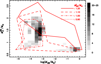
Figure 18: The distribution of the CE mass and the companion mass when $M_{\rm WD}=1.378\,M_{\odot}$, and the contour in the ($M_{\rm CE}$-$M_{\rm 2}^{\rm SN}$) plane for different initial WD masses. Here, we only show the case of $\alpha_{\rm CE}=1.0$ since the contours for the case of $\alpha_{\rm CE}=3.0$ are very similar.

5.2 The CE mass at the time of the supernova explosion

Fig. 7 shows that some SNe Ia can explode in the CEW phase, i.e. there is still some material in the CE when $M_{\rm WD}=1.378\,M_{\odot}$, which could affect the observational properties of SNe Ia. This is the most significant difference between the CEW and the OTW model. Fig. 18 shows the distribution of the CE mass and the companion mass when $M_{\rm WD}=1.378\,M_{\odot}$ and the contour of the CE mass and the companion mass in a $M_{\rm 2}^{\rm SN}-\log(M_{\rm CE})$ plane. Here, we only show the case of $\alpha_{\rm CE}=1.0$ since the case of $\alpha_{\rm CE}=3.0$ is similar. Roughly 1.2%$-$14.2% of all SNe Ia explode in the CEW phase, which depends on the value of $\alpha_{\rm CE}$. The percentage for which SNe Ia explode in the CEW phase in the CEW model is slightly larger than the one for which SNe Ia explode in the OTW phase in the OTW model (Meng et al. 2010; Meng & Yang 2011b). The CE mass ranges from $10^{\rm-5}\,M_{\odot}$ to $\sim 1\,M_{\odot}$. For most cases, the CE mass lies between a few $10^{\rm-4}\,M_{\odot}$ and a few $10^{\rm-3}\,M_{\odot}$. It may be difficult to detect such hydrogen-rich material directly; however, such low-mass CEs might leave footprints in the high-velocity features in the spectrum of SNe Ia (Mazzali et al. 2005a, b).

In some cases, the CE mass can be larger than 0.1 $M_{\odot}$, even as large as 1 $M_{\odot}$. If the SNe Ia occurs in such situations, hydrogen lines should easily be detectable in the early spectra of some SNe Ia. While such strong hydrogen lines were indeed discovered in some SNe Ia, such as SN 2002ic (Hamuy et al. 2003), this is not consistent with observations of most SNe Ia. This may require a time delay between the moment when $M_{\rm WD}=1.378\,M_{\odot}$ and the supernova explosion; this time needs to be long enough so that the CE material can be lost. Based on the CE mass and the mass-reduction rate of the CE, we estimate that at least a few $10^{\rm 5}$ yr is needed for such a delay time. Obviously, a simmering phase, lasting $\sim 10^{\rm 3}$ yr, of the WD before the supernova explosion does not produce such a delay time (Piro & Chang P. 2008; Chen et al. 2014). A possible suggested mechanism is provided by the spin-up/spin-down model (Justham 2011; Di Stefano & Kilic 2012), where the WD is spun up by accretion. If the resulting WD’s rotation velocity is sufficiently large, the WD may not explode as a SN Ia even when its mass exceeds 1.378 $M_{\odot}$. Hence to explode, a spin-down phase of the WD is required. During the spin-down phase, the companion may lose almost all of its hydrogen-rich envelope and become a very faint object. Such a mechanism may explain the lack of hydrogen lines in the late-time spectrum of SNe Ia predicted by the interaction between the supernova ejecta and a hydrogen-rich companion, and why no surviving companion has been found, e.g., in the supernova remnant SNR 0509-67.5 (Justham 2011; Di Stefano & Kilic 2012). However, from a purely theoretical point of view, it is completely unclear how long the spin-down timescale is (Di Stefano et al. 2011). Recently, based on the observational fact that CSM exists around some SNe Ia, Meng & Podsiadlowski (2013) provided a constraint on the spin-down timescale using a semi-empirical method; they found that the spin-down timescale should be shorter than a few $10^{\rm 7}$ yr, otherwise it would be impossible to detect the signature of the CSM. Such a timescale is long enough to erase most of the possible observational signatures predicted by the SD model, but short enough that it does not affect the delay time of supernova explosions since the formation of the primordial system formation. $10^{\rm 5}$ yr is needed for our CEW model to fulfill the constraint in Meng & Podsiadlowski (2013). Because of the possibility of relatively massive initial companions (in the top right corner in Fig. 7), the delay time for SNe Ia exploding in the CE phase with $M_{\rm CE}>0.1\,M_{\odot}$ ranges from 240 Myr to 330 Myr. We estimate that no more than 1.7 in 100 SNe Ia belong to this subclass. Those SNe Ia exploding in massive CEs may contribute to 2002ic-like SNe Ia since their birth rate and delay time is consistent with those estimated from observations, and a strong hydrogen line is expected from the interaction between the supernova ejecta and a massive CE (Aldering et al. 2006).

In Fig. 18, there is a gap in the distribution of $M_{\rm CE}$, which is mainly caused by the different evolutionary stages of the companion stars at the onset of RLOF which sets the mass-transfer timescale. Generally, the mass-transfer timescale for companion stars more massive than $\sim 2~{}M_{\odot}$ does not vary monotonically with evolutionary stage from the zero-age main sequence to the bottom of the RGB (Podsiadlowski et al. 2002). Consequently, the critical mass ratio for dynamically unstable mass transfer also does not vary monotonically with the evolutionary stage, which itself is determined by the orbital period of the system at the beginning of RLOF (Ge et al. 2015). Generally, for a given binary system, a longer mass-transfer timescale means a lower average mass-transfer rate. If RLOF begins when the companion crosses the HG, the exact evolutionary stage which gives the longest mass-transfer timescale depends on the initial companion mass. Systems with the longest mass-transfer timescale are more likely to be found in the SSS phase when $M_{\rm WD}=1.378~{}M_{\odot}$ rather than in the CEW phase, although systems with the same initial WD and companion masses but with shorter or longer orbital periods may explode in the CEW phase or experience a delayed dynamical instability (see panel (7) in Fig. 7).

For those with longer orbital periods, the mass-transfer timescale sharply decreases with orbital period, which results in a very high mass-transfer rate; then the CE mass may be larger than $0.1~{}M_{\odot}$ at the time of the supernova explosion, an example of which is shown in Fig. 4. In addition, for very high mass-transfer rates, the companion will lose its outer envelope quickly. With the loss of the companion’s envelope, the hydrogen fraction of the transferred material decreases, which results in a higher critical accretion rate and hence a higher mass-growth rate of the CO WD (see equation (12) and panels (2) and (3) in Fig. 4). So, the time from the onset of RLOF to the moment of the supernova explosion is shortened; this also contributes to the population of SNe with massive CEs as the timescale for losing the CE is also shortened. However, such cases only occur for systems with initial WD masses $\geq 1.1~{}M_{\odot}$ and relatively massive companions.

For those with shorter initial orbital periods, the mass-transfer timescale may become so short that the systems experience a delayed dynamical instability if the mass ratio of the donor star to the WD is sufficiently high. Such systems may eventually merge and hence not contribute to the SN Ia population. If the mass ratio is not very high, the mass-transfer timescale of the systems with a shorter initial orbital period will become shorter, but not much shorter than the longest mass-transfer timescale. This implies a relatively higher, but not much higher mass-transfer rate. So, a massive CE is difficult to maintain for very high mass-loss rates from the surface of the CE. Even for the cases almost experiencing a delayed dynamical instability, the massive CE can also not be maintained for a long time (see also Fig. 6). At the moment when $M_{\rm WD}=1.378~{}M_{\odot}$, the mass-transfer rate of these systems is generally slightly larger than the critical accretion rate, which means that the CE cannot be very massive, e.g. $\leq 10^{\rm-3}~{}M_{\odot}$. Additionally, the failure to maintain a massive CE at the time of the supernova explosion is also partly caused by the relatively longer mass-growth timescales of the WDs, even for systems with the same initial WD mass, due to the unchanged hydrogen mass fraction (see the different explosion times in Figs. 4 and 6). SNe Ia that explode in a low-mass CE predominantly occur for systems with initial WD masses $\leq 1.0~{}M_{\odot}$, where the mass-growth timescale of the WDs is too long to maintain a very massive CE at the time of the explosion. Therefore, if a system explodes in the CEW phase, the CE tends to have a mass of either $\leq 10^{\rm-3}~{}M_{\odot}$ or $\geq 0.1~{}M_{\odot}$, which leads to the gap in the distribution of $M_{\rm CE}$. Moreover, as clearly shown by the red and green points at the bottom of panel (7) in Fig. 9, the companions for those WDs exploding in a high-mass CE are less massive than the ones exploding in a low-mass CE.

Figure 19: Similar to Fig. 4 but for a different average CE density. The average density from equation (6) is arbitrarily multiplied by a factor of 0.1 (top four panels) and 10 (bottom four panels).

6 Discussion

6.1 Uncertainties in the CEW model

In this paper, we constructed a new SD model in which a CE forms around the binary when the mass-transfer rate exceeds the critical accretion rate. Material in the CE is lost from the surface of the CE instead from the WD surface in the OTW model. Many of the results in the CEW model are similar to those in the OTW model, such as the evolution of binary parameters, while the parameter space leading to SNe Ia and the birth rate of SNe Ia in the CEW model are somewhat larger than in the OTW model. However, the CEW model as presented in this paper is still very simple at present with numerous uncertainties in the detailed modelling. In the following, we discuss some of the main uncertainties in our new CEW models one by one.

In the CEW model, one of the main uncertainties arises from the assumed CE density. In this paper, we simply assumed that the CE is spherical and used an average density to replace the density at the boundary of the inner and the outer part of the CE. The density $\rho$ directly affects the effective turbulent viscosity (equation 3), and hence the angular-momentum loss from the binary system, the frictional luminosity and consequently the mass loss from the system. To test the effect of varying the CE density on the final parameter contours leading to SNe Ia, we arbitrarily multiplied the density in equation (6) by factors of 0.1 and 10, respectively, and recalculated the contour leading to SNe Ia for $M_{\rm WD}^{\rm i}=1.1\,M_{\odot}$. Fig. 19 provides an example to show how the average density affects the binary evolution. The figures show that, as one might expect, a higher average density results in a higher frictional luminosity and a higher mass-transfer rate, and hence leads to a more massive CE. If the average density is high enough, i.e. the density is increased by a factor of 20 or larger, the system will experience a dynamical instability and the system will eventually merge. The critical density factor is system-dependent. For example, for the system with ($M_{\rm WD}^{\rm i}/M_{\odot}$, $M_{\rm 2}^{\rm i}/M_{\odot}$, $\log(P^{\rm i}/{\rm d})$) = (0.8, 2.2, 0.4), the critical density factor is 250 due to a much less massive CE. In addition, the evolutionary track of the companion in the HR diagram is significantly affected by the frictional density, as is the period. Fig. 20 shows how the density factor affects the final state of the binary system when $M_{\rm WD}=1.378\,M_{\odot}$: the companion mass, orbital period and the mass-transfer timescale decrease, while the CE mass increases with the density factor. This is a direct consequence of the higher frictional luminosity as this leads to a larger loss of orbital angular momentum due to the friction between the binary system and the CE; this leads to a higher mass-transfer rate and a more massive CE. At the same time, the companion will lose more material and becomes less massive, i.e. may be as small as 0.5 $M_{\odot}$ at the time when $M_{\rm WD}=1.378$ $M_{\odot}$. Due to the relatively small radius for the shorter orbital period, the companion also has a low luminosity, i.e. is dimmer than $1\,L_{\odot}$. The relatively short mass-transfer timescale for a large density factor here is a direct consequence of equation (12). A high density factor results in a higher mass-transfer rate, and the companion will lose its outer envelope more quickly. With the loss of the companion’s envelope, the hydrogen fraction of the transferred material decreases; this leads to a higher critical accretion rate and a higher mass-growth rate of the CO WD (see panels 2 and 3 in Figs. 4 and 19) and a shorter overall mass-transfer timescale. The influence of high density on the companion could provide some clues in searches for surviving companions in supernova remnants, e.g. a dim MS star with a relatively low surface hydrogen fraction.

However, we find that the contours leading to SNe Ia in the ($\log P_{\rm i},M_{\rm 2}^{\rm i}$) planes for different average densities is more or less the same as that shown in Fig. 8, irrespective of the density factor, except that more SNe Ia explode in the CE phase for a higher assumed CE density. As shown in Fig. 20, the higher the frictional density, the more massive the CE, making it more likely that the supernova explodes in the CE phase. As far as the contours resulting in SNe Ia is concerned, only the upper boundary, which is determined by systems that experience a delayed dynamical instability, would be significantly affected by the frictional density. For a given system, the higher the frictional density, the more likely the system experiences a delayed dynamical instability, moving the upper boundary downwards. However, as discussed above, although this is model-dependent, only when the density factor is larger than $\simeq 20$ would systems that avoid the merging fate in our standard model experience a delayed dynamical instability. Therefore, within the density range tested here, the upper boundaries of the contours are almost unaffected by the density factor. The left and right boundaries are determined by the radius of stars on the ZAMS, or at the the end of the HG, which are completely unaffected by the density factor. The lower boundary is constrained by the condition that the secondaries are massive enough to increase the WD mass to $1.378~{}M_{\odot}$. This condition is very weakly dependent on the frictional density factor as discussed above for a system with ($M_{\rm WD}^{\rm i}/M_{\odot}$, $M_{\rm 2}^{\rm i}/M_{\odot}$, $\log(P^{\rm i}/{\rm d})$) = (0.8, 2.2, 0.4).

Figure 20: The companion mass, orbital period, CE mass and mass-transfer timescale (from the onset of RLOF to the supernova explosion) when $M_{\rm WD}=1.378\,M_{\odot}$ as a function of the density factor, where the initial parameter of the model is ($M_{\rm WD}^{\rm i}/M_{\odot}$, $M_{\rm 2}^{\rm i}/M_{\odot}$, $\log(P^{\rm i}/{\rm d})$)=(1.1, 3.3, 0.6).

Another key uncertainty arises from the adopted mass-loss rate from the surface of the CE, which determines the mass left in the CE; there is no well established prescription for mass loss from a CE (cf. Schröder & Cuntz 2007). Here, we again arbitrarily multiply the mass-loss rate in equation (8) by a factor of 0.1 or 10. Fig. 21 shows an example of how the mass-loss rate affects the binary evolution and the final state of the binary system. Figs. 4 and 21 show that the wind mass-loss rate does not affect the binary evolution as significantly as the density does, while it may influence the CE mass considerably. There is a clear trend that, for a lower wind mass-loss rate, WDs tend to reach 1.378 $M_{\odot}$ during the CE phase, while WDs are more likely to explode in the SSS or RN phase for the higher mass-loss rates. In other words, for a higher mass-loss rate, it becomes more difficult to maintain the CE while it is relative easy to obtain a more massive CE for a lower mass-loss rate. In fact, when the wind enhancement factor is larger than 10, the effect of the CE wind on the evolution of the binary is rather minor, and the evolution is very similar to that of the OTW. However, the WD may gradually increase its mass to 1.378 $M_{\odot}$ for any mass-loss rate. Fig. 22 shows how the wind enhancement factor affects the final state of the binary system. The wind mass-loss rate only has a minor effect on the SN formation rate when the wind mass-loss rate is sufficiently low (the wind factor is lower than 0.1), although a lower wind factor favours the existence of the CE. This directly follows from equation (7), i.e. $\dot{M}_{\rm CE}=|\dot{M}_{\rm 2}|-\dot{M}_{\rm WD}-\dot{M}_{\rm wind}\simeq|\dot{M}_{\rm 2}|-\dot{M}_{\rm WD}$ when the wind mass-loss rate is much lower than $\dot{M}_{\rm 2}$ and $\dot{M}_{\rm WD}$ and can therefore be neglected. Thus, if the wind factor is low enough, the evolution of the CE no longer depends on the mass-loss rate.

Fig. 23 presents a map for SNe Ia and mergers in the density – wind factor plane; the boundary between SNe Ia and mergers is also shown in the figure. The figure illustrates that the boundary is system-dependent, especially for the density factor. However, for a rather large parameter region, binary systems may avoid the fate of merging, demonstrating that the CEW model is rather robust.

Figure 21: Similar to Fig. 4 but for a different mass-loss rate. The mass-loss rate from equation (8) is arbitrarily multiplied by a factor of 0.1 (top four panels) or 10 (bottom four panels).

The factor $\alpha$ in Equation (1) is also an important factor which directly affects the orbital angular-momentum loss and the frictional luminosity. Its influence on the binary evolution is quite similar to the changes in the frictional density as already discussed above.

In this paper, we assumed that all the potential energy sources, i.e. from nuclear burning, the secondary’s luminosity and the frictional luminosity are contributing to driving the wind mass loss. A small part of that energy will be required to drive the expansion of the CE itself, which could moderately decrease the expected mass loss. However, as we discussed above, there is a rather large parameter range for which the assumptions about the wind do not affect whether a binary system explodes as a SN Ia or not. Therefore, this effect is unlikely to change the main conclusions of this paper.

We also assumed that the presence of an envelope changes the helium flash at the bottom of the hydrogen-burning shell like in a TPAGB star. On the other hand, if the CE is not massive enough and the helium flash is strong enough, the CE might be destroyed. We plan to study the conditions for which the destruction of the CE can be prevented in the future.

Finally, for the CEW model it is still unclear what the system actually would look like during the CE phase; this will depend on the CE mass, the nuclear luminosity for hydrogen and helium burning and the percentage of the total energy used to drive the mass loss from the surface of the CE. In general, we would expect a RG-like object with a high luminosity. We will address this issue in the future following the approach developed previously in Podsiadlowski et al. (1990).

In summary, our CEW model as it stands now is still very simple, but most of our assumptions are rather conservative. We therefore consider the results in this paper only as the first step and we intend to refine the model in the future.

6.2 The differences between the CEW model and the OTW model

The physical assumptions in the CEW model and the OTW model are quite different, which should lead to several testable differences between the two models.

1) The CEW model does not directly depend on metallicity; hence it allows SNe Ia to occur in any environment irrespective of metallicity and redshift. Thus, the discovery of some SNe Ia at high redshifts and/or in a low-metallicity environment are easily explained in the CEW model. The lack of a low-metallicity threshold for SNe Ia relative to SNe II is also a natural result in the CEW model.

2) When $|\dot{M}_{\rm 2}|$ exceeds $\dot{M}_{\rm cr}$, the hydrogen-rich material burns stably on the WD at a rate of $\dot{M}_{\rm cr}$, while the unprocessed material forms the CE. At the same time, some CE material may leave the system from the surface of the CE. This treatment leads to two significant differences between the CEW model and the OTW model. One is that the mass-growth rate of the WD in the CEW model is larger than that in the OTW model, which results in a larger initial parameter space for SNe Ia and a lower minimum WD mass, and hence a higher birth rate. The other is the wind velocity. In the CEW model, the unprocessed material leaves the system from the surface of the CE instead of the surface of the WD, resulting in a much lower wind velocity than in the OTW model, i.e. most likely less than 200 ${\rm km}\,{\rm s}^{\rm-1}$, probably lower than 50 ${\rm km}\,{\rm s}^{\rm-1}$. Our model is therefore compatible with the dynamics of the forward shock and the X-ray emission from the shocked ejecta in SN Ia remnants examined by Badenes et al. (2007). Even the properties of RCW 86, where the wind cavity with a diameter of $\sim 30$ pc contains 1.6 $M_{\odot}$ of material ejected from the progenitor system (Broersen et al. 2014), may be explained by our model since a low-density cavity around some SNe Ia could also be expected for some cases in our model grid (see Fig. 15).

3) When the hydrogen-rich material is stably burning on the surface of the WD, soft X-ray emission is expected from the mass-accreting WD and the system will appear as a supersoft source (SSS, van den Heuvel 1992), while no strong X-ray emission is expected from the DD scenario until just before the SN Ia explosion. This provides a potential method for distinguishing between SD and DD models. However, the number of the SSSs in elliptical and spiral galaxies is much smaller than that predicted from the standard SD model (Gilfanov & Bogdán 2010; Di Stefano 2010). The predicted number of SSSs from the SD model in these studies is based on the assumption that all the accreting WDs are in the SSS phase which lasts for about two million years before the SN Ia explosion. This assumption is rather simple and may overestimate the duration of the SSS phase by a factor of 10 (see panel 3 in Figs 2 and 4). According to the OTW model, in which the OTW may absorb the soft X-rays, the duration of the SSS phase is much shorter; Hachisu et al. (2010c) and Meng & Yang (2011b) were able to reproduce the observed SSS number in elliptical and spiral galaxies, i.e. only a small fraction of mass-accreting WDs resulting in SNe Ia contribute to the supersoft X-ray flux of a galaxy. In the CEW model, because of the existence of the CE, X-rays would be completely absorbed by the CE or the material lost from the CE surface. The duration of the SSS phase in the CEW model would be even shorter than in the OTW model since, even when $|\dot{M}_{\rm 2}|$ is smaller than $\dot{M}_{\rm cr}$, a CE can still exist (see the panel 3 in Fig. 4). So, the CEW model is likely to be consistent with the observations of Gilfanov & Bogdán (2010) and Di Stefano (2010) (also see the discussion about the SSS phase in Maoz, Mannucci & Nelemans 2014).

4) The OTW model may explain the properties of some RNe which have been suggested as potential progenitors of SNe Ia (Hachisu & Kato 2005, 2006a, 2006b; Hachisu et al. 2007); this also applies to the CEW model as the CEW model reduces to the OTW model when there is no CE.

Figure 22: The companion mass, orbital period, CE mass and mass-transfer timescale (from the onset of RLOF to the supernova explosion) when $M_{\rm WD}=1.378\,M_{\odot}$ as a function of the wind factor, where the initial parameter of the model is ($M_{\rm WD}^{\rm i}/M_{\odot}$, $M_{\rm 2}^{\rm i}/M_{\odot}$, $\log(P^{\rm i}/{\rm d})$)=(1.1, 3.3, 0.6).

Figure 23: The map for SNe Ia and mergers in the density – wind factor plane (for a representative system with initial parameters of ($M_{\rm WD}^{\rm i}/M_{\odot}$, $M_{\rm 2}^{\rm i}/M_{\odot}$, $\log(P^{\rm i}/{\rm d})$)=(1.1, 3.3, 0.6) and (0.8, 2.2, 0.4), respectively). Stars represent systems that explode as SNe Ia, while crosses indicate systems that merge. The solid and dashed curves show the boundary between SNe Ia and mergers obtained from the systems of (1.1, 3.3, 0.6) and (0.8, 2.2, 0.4), respectively.

Figure 24: Contours leading to SNe Ia in the secondary mass – orbital period plane for $M_{\rm WD}^{\rm i}=1.0\,M_{\odot}$. The solid curve is for $\eta_{\rm He}$ in Kato & Hachisu (2004) and the dashed curve is for $\eta_{\rm He}$ arbitrarily increased by 50 %, i.e. $\eta_{\rm He}^{\rm{}^{\prime}}=\min(1,1.5\eta_{\rm He})$.

5) The efficiency of the accretion of hydrogen on massive WDs at a high rate over many cycles is still controversial; this affects the conditions for which SNe Ia can occur. For example, Idan (2013) recently concluded that the accumulated helium under the hydrogen-burning shell is completely lost in a strong helium flash, which, taken at face value, would make SNe Ia impossible. On the other hand, Newsham (2014) conclude that a WD may continue to increase its mass toward the Chandrasekha limit. The helium accumulation efficiency, $\eta_{\rm He}$, used here is usually smaller than 1 even when hydrogen burns at a rate of $\dot{M}_{\rm cr}$. Fortunately, although it is not clear how the WD adjusts to alternating helium flashes and stable hydrogen shell burning in the OTW model, this issue probably does not arise in the CEW model. In addition, $\eta_{\rm He}$ could be larger than derived by Kato & Hachisu (2004) if the effect of H shell burning has been accounted for, since the nuclear energy produced via H-burning keeps the underlying He buffer hotter, resulting in weaker and more frequent He flashes (Cassisi et al. 1998). Especially, Hillman et al. (2016) recently found that, although a significant fraction of the material accumulated prior to the flash is lost during the first few helium shell flashes, the fraction decreases with repeated helium shell flashes and eventually no mass is lost at all during subsequent flashes. In addition, the helium shell flash in a rapidly rotating WD due to accretion will become more stable than in the corresponding non-rotating WD (Yoon & Langer 2004a, b). We tested the effect of the accumulation efficiency of helium flashes on the parameter space leading to SNe Ia by increasing $\eta_{\rm He}$ by 50% rather arbitrarily (but keeping the maximum value of $\eta_{\rm He}$ at 1). Fig. 24 shows a comparison of the contours leading to SNe Ia for different values of $\eta_{\rm He}$. The figure shows that a higher $\eta_{\rm He}$ moves the lower boundary to a lower value while the other boundaries are almost unaffected by a change of $\eta_{\rm He}$. The reason is that $\eta_{\rm He}$ only plays a role in phases of stable burning or weak hydrogen flashes (see Fig. 7). In addition, for a lower initial WD mass ($<0.9\,M_{\odot}$), most SNe Ia explode in the SSS or RN phase, where $\eta_{\rm He}$ may play a more important role, i.e. a high $\eta_{\rm He}$ results in a larger parameter space for SNe Ia. So, a higher $\eta_{\rm He}$ could lead to a relatively higher birth rate of SNe Ia and produce SNe Ia in an older population.

6) As far as the possible appearance of a WD in the OTW phase is concerned, Nomoto et al. (2007) suggested that the system might look like an undersized OB star, i.e. with an effective temperature of $31600-10000$ K, but with a size of only a few $R_{\odot}$, limited by the WD’s RL radius. However, no such rapidly accreting blue white dwarf has been found in searches in the Large Magellanic Cloud (Lepo & van Kerkwijk 2013a). Alternatively such systems might look like Wolf-Rayet (WR) stars or WD planetary nebulae (see also Lepo & van Kerkwijk 2013a; Nielsen et al. 2013; Wheeler & Pooley 2013). It is worth emphasizing that, for most cases, when the mass-transfer rate is very high, i.e. higher than $10^{\rm-5}\,M_{\odot}$ yr^-1 (see Han & Podsiadlowski 2004 and Meng et al. 2009a), the OTW must carry away a large amount of dynamic energy which almost equals the nuclear burning energy. So, during the OTW phase, the WD must be dimmer. In the CEW model, we suggest that the system resembles a TPAGB star during the CE phase. If the system loses the envelope before the supernova, it could look like a post-AGB star. After the CE phase, the accreted hydrogen-rich material burns stably on the surface of the WD, and the system may show the properties of a SSS, which is a powerful source of ionizing ultraviolet emission. Such ultraviolet photons may ionize helium in the CSM or interstellar medium, and then emission in the recombination lines of HeII could be expected. Interestingly, searching for the recombination radiation of HeII in passively evolving galaxies, Johansson et al. (2014) found that the strength of the observed HeII $\lambda$4686 nebular emission is consistent with the post-AGB stars being the sole ionizing source. In addition, during the CE phase, if the envelope is massive enough, a high luminosity, i.e. even higher than the Eddington luminosity of the WD, and a variable high mass-loss rate for helium flashes might be expected. LMC N66 in the Large Magellanic Cloud could be an interesting candidate: it consists of a WD primary and a non-degenerate system in the center and experiences huge mass loss with a highly variable mass-loss rate (Lepo & van Kerkwijk 2013b). In any case, it is still unclear how to distinguish these from real TPAGB stars, and a detailed study on the appearance of the binary system for our CEW model is still required. We have started such an investigation and will report the results in a future publication.

7) One question that has been raised for a long time since Hachisu et al. (1996, 1999b) is whether the OTW model requires too much fine-tuning (e.g. Piersanti et al. 2000; Shen & Bildsten 2007; Woosley & Kasen 2011). In contrast, as discussed in section 6.1, our CEW model is rather robust and may work within a very large parameter range, probably requiring much less fine-tuning (see Fig. 23).

7 Summary and conclusion

We have constructed a new SD model for SNe Ia in which a common envelope forms when the mass-transfer rate onto the WD exceeds a critical accretion rate instead of an optically thick wind. Based on the CEW model, we investigated in detail the WD+MS channel using detailed binary evolution calculations. The initial parameters for SNe Ia in the ($\log P^{\rm i},M_{\rm 2}^{\rm i}$) plane were obtained and then used to study the evolution of the birth rate of SNe Ia by a BPS method. In the following we summarize the main results.

1) The parameter space obtained from our new CEW model is slightly larger than that in the OTW model, i.e. it allows a higher initial companion mass and longer initial orbital period. The minimum WD mass leading to SNe Ia is 0.65 $M_{\odot}$, slightly lower than in the OTW model.

2) We also presented the final parameters of the binary systems and the companion properties at the time of the supernova explosion, which may be helpful for identifying progenitor systems or search for surviving companions in supernova remnants. Several observed SSSs and RN systems lie in the parameter regions for SNe Ia, making them ideal candidates for SN Ia progenitors. The properties of Tycho G, the suggested surviving companion of Tycho’s supernova, is also consistent with our results.

3) Before the SN Ia explosion, the system may lose as much as 2.5 $M_{\odot}$ of hydrogen-rich material, where there is a trend that, the more mass is lost, the closer the maximum distance this material may reach. For some SNe Ia, the material may be less than 0.2 $M_{\odot}$, spread over a very large region, possibly extending to more than 300 pc. The environment around these SNe Ia could be very clean and it would be very difficult to detect a signature of this CSM around such SNe Ia.

4) A significant fraction of SNe Ia may explode in the CE phase with a CE mass from a few $10^{\rm-4}\,M_{\odot}$ to a few $10^{\rm-3}\,M_{\odot}$; these might be essential for explaining the high-velocity Ca features seen in the spectrum of SNe Ia (Mazzali et al. 2005a, b).

5) For a single star burst, most SNe Ia occur between 0.25 Gyr and 2 Gyr, while the Galactic birth rate of the SNe Ia from our CEW model is (0.89-1.20)$\times 10^{\rm-3}\,{\rm yr^{\rm-1}}$, which is higher than in the OTW model by about $\sim 30\,$%.

6) We examined the uncertainties of our model caused by uncertainties in the modeling parameters and found that the model is very robust within a very large parameter range.

7) We discussed the differences between the CEW and the OTW model. Our model avoids several of the shortcomings of the OTW model but also shares the merits of the OTW model. Especially, our model does not depend on metallicity, and SNe Ia may occur in low-metallicity and/or high-redshift environments. In addition, the typical outflow velocity should be much lower than in the OTW model since the material is lost from the CE surface instead of the WD surface in the OTW model.

8) The accumulation efficiency for helium flashes could be a very important factor in determining the parameter space that leads to a successful SN Ia, i.e.  a higher $\eta_{\rm He}$ than in Kato & Hachisu (2004) may extend the allowed range of companion masses to a lower initial mass, resulting in a higher birth rate and a possibly longer delay time.

9) Our model may naturally explain the birth rate and delay time of 2002ic-like SNe Ia.

Appendix A The method for calculating the CE mass in our code

In section 2.2, equations (7), (8), (10) and (11) form a coupled set of equations that determine the mass in the CE. Here, we show how this is determined in our code. The main idea is that the formation of the CE and the mass loss from the CE surface may be divided into two steps, i.e. the CE forms first, and then the wind begins to blow. In our code, there is a transition value $M_{\rm CE}^{{}^{\prime}}$, which is determined by

$$M_{\rm CE,i+1}^{{}^{\prime}}=M_{\rm CE,i}+(|\dot{M}_{\rm 2}|_{\rm i}-\dot{M}_{\rm WD,i})\cdot\Delta t,$$ (23)

where the initial value of $M_{\rm CE,0}=0$. Then, putting the transition value into Equation (10), we may get the CE radius. Based on equations (3), (5) and (6), the frictional luminosity $L_{\rm f}$ may be obtained, and then the total luminosity $L_{\rm tot}=L_{\rm nuc}+L_{\rm 2}+L_{\rm f}$, where $L_{\rm nuc}$ is nuclear energy for stable hydrogen burning and $L_{\rm 2}$ is the secondary luminosity. $L_{\rm nuc}$ is obtained from equation (9). Therefore, according to Equation (8), we may get the mass-loss rate $\dot{M}_{\rm wind}$, where the CE mass is also the transition value from Equation (23). The CE mass is then calculated according to

$$M_{\rm CE,i+1}=M_{\rm CE,i+1}^{{}^{\prime}}-\dot{M}_{\rm wind,i}\cdot\Delta t.$$ (24)

Equation (23) + Equation (24) deduces to

$$\begin{array}[]{lc}M_{\rm CE,i+1}=M_{\rm CE,i}+(|\dot{M}_{\rm 2}|_{\rm i}-\dot{M}_{\rm WD,i}-\dot{M}_{\rm wind,i})\cdot\Delta t\\ \\ \hskip 35.56593pt=M_{\rm CE,i}+\dot{M}_{\rm CE,i}\cdot\Delta t,\end{array}$$ (25)

which is exactly the same as Equation (11).

References

- Aldering et al. (2006) Aldering G., Antilogus P., Bailey S. et al., 2006, ApJ, 650, 510
- Alexander & Ferguson (1994) Alexander D. R., Ferguson J. W., 1994, ApJ, 437, 879
- Arnett (1982) Arnett W.D., 1982, ApJ, 253, 785
- Badenes et al. (2007) Badenes C., Hughes J.P., Bravo E., Langer N., 2007, ApJ, 662, 472
- Badenes & Maoz (2012) Badenes C., Maoz D., 2012, ApJL, 749, L11
- Bedin et al. (2014) Bedin L.R., Ruiz-Lapuente P., González Hernández J.I. et al., 2014, MNRAS, 439, 354
- Blondin et al. (2009) Blondin S., Prieto J.L., Patat F. et al., 2009, ApJ, 693, 207
- Borkowskin et al. (2006) Borkowski K.J., Hendrick S.P., Reynolds S.P., 2006, ApJ, 652, 1259
- Borkowskin et al. (2009) Borkowski K.J., Blondin J.M., & Reynolds S.P., 2009, ApJ, 699, L64
- Brown (2014) Brown, P. J. 2014, ApJ, 796, L18
- Branch et al. (1995) Branch D., Livio M., Yungelson L.R. et al., 1995, PASP, 107, 1019
- Branch (2004) Branch D., 2004, Nature, 431, 1044
- Broersen et al. (2014) Broersen S., Chiotellis A., Vink J., Bamba A., 2014, MNRAS, 441, 3040, arXiV: 1404.5434
- Cao et al. (2015) Cao Y., Kulkarni S. R., Howell D. A., et al. 2015, Nature, 521, 328
- Cao et al. (2016) Cao Y., Kulkarni S.R., Gal-Yam A., et al., 2016, ApJ, 832, 86, arXiv: 1606.5655
- Cappellaro & Turatto (1997) Cappellaro E., Turatto M., 1997, in Ruiz-Lapuente P., Cannal R., Isern J., eds, Thermonuclear Supernovae. Kluwer, Dordrecht, p. 77
- Cassisi et al. (1998) Cassisi S., Iben I. Jr., Tornambè A., 1998, ApJ, 496, 376
- Chen & Han (2002) Chen X., Han, Z., 2002, MNRAS, 335, 948
- Chen & Han (2003) Chen X., Han, Z., 2003, MNRAS, 341, 662
- Chen & Tout (2007) Chen X., Tout C.A., 2007, ChJAA, 7, 2, 245
- Chen & Han (2008) Chen X., Han, Z., 2008, MNRAS, 387, 1416
- Chen et al. (2011) Chen X., Han Z., Tout C.A., 2011, ApJ, 735, L31
- Chen et al. (2014) Chen X., Han Z., Meng, X., 2014, MNRAS, 438, 3358
- Chen & Li (2007) Chen W., Li X., 2007, ApJ, 658, L51
- Chomiuk (2013) Chomiuk L., 2013, PASA, 30, 46
- Di Stefano & Kong (2003) Di Stefano R., Kong A.K.H., 2003, ApJ, 592, 884
- Di Stefano (2010) Di Stefano R., 2010, ApJ, 712, 728
- Di Stefano et al. (2011) Di Stefano R., Voss R., & Claeys J.S.W., 2011, ApJL, 738, L1
- Di Stefano & Kilic (2012) Di Stefano R., & Kilic M. 2012, ApJ, 759, 56
- Dilday et al. (2012) Dilday B., Howell D.A., Cenko S.B. et al., 2012, Science, 337, 942
- Eggleton (1971) Eggleton P.P., 1971, MNRAS, 151, 351
- Eggleton (1972) Eggleton P.P., 1972, MNRAS, 156, 361
- Eggleton (1973) Eggleton P.P., 1973, MNRAS, 163, 279
- Eggleton et al. (1989) Eggleton P. P., Tout C. A., Fitechett M. J., 1989, ApJ, 347, 998
- Frederiksen et al. (2012) Frederiksen T.F., Hjorth J., Maund J.R. et al., 2012, ApJ, 760, 125
- Fuhrmann (2005) Fuhrmann K., 2005, MNRAS, 359, L35
- Foley et al. (2012) Foley, R. J., Challis, P. J., Filippenko, A. V., et al. 2012, ApJ, 744, 38
- Galbany et al. (2016) Galbany L. Stanishev V. Mourão A. M. et al., 2016, A&A, 591, A48
- Ge et al. (2015) Ge H., Webbink R. F., Chen X., Han Z., 2015, ApJ, 812, 40
- Ghavamian et al. (2001) Ghavamian P., Raymond J., Smith R.C., Hartigan P., 2001, ApJ, 547, 995
- Gilfanov & Bogdán (2010) Gilfanov M. & Bogdán A., 2010, Nature, 463, 924
- Goldberg & Mazeh (1994) Goldberg D., Mazeh T., 1994, A&A, 282, 801
- González-Hernández et al. (2009) González-Hernández J, Ruiz-lapuente P, Filippenko A, et al., ApJ, 2009, 691, 1
- Graur et al. (2016) Graur O., Zurek D., Shara M.M., et al., 2016, ApJ, 819, 31
- Greggio & Renzini (1983) Greggio L., Renzini A., 1983, A&A, 118, 217
- Hachisu et al. (1996) Hachisu I., Kato M., Nomoto K., ApJ, 1996, 470, L97
- Hachisu et al. (1999a) Hachisu I., Kato M., Nomoto K., Umeda H., 1999a, ApJ, 519, 314
- Hachisu et al. (1999b) Hachisu I., Kato M., Nomoto K., 1999b, ApJ, 522, 487
- Hachisu & Kato (2000) Hachisu I., Kato M., 2000, ApJ, 540, 447
- Hachisu et al. (2000a) Hachisu I., Kato M., Kato T., Matsumoto K., 2000a, ApJ, 528, L97
- Hachisu et al. (2000b) Hachisu I., Kato M., Kato T., Matsumoto K., Nomoto K., 2000b, ApJ, 534, L189
- Hachisu et al. (2010c) Hachisu I., Kato M., Nomoto K., 2010c, ApJL, 724, L212
- Hachisu & Kato (2001) Hachisu I., Kato M., 2001, ApJ, 558, 323
- Hachisu et al. (2003) Hachisu I., Kato M., Schaefer B.E., 2003, ApJ, 584, 1008
- Hachisu & Kato (2003a) Hachisu I., Kato M., 2003a, ApJ, 588, 1003
- Hachisu & Kato (2003b) Hachisu I., Kato M., 2003b, ApJ, 590, 445
- Hachisu & Kato (2005) Hachisu I., Kato M., 2005, ApJ, 631, 1094
- Hachisu & Kato (2006a) Hachisu I., Kato M., 2006a, ApJ, 642, L52
- Hachisu & Kato (2006b) Hachisu I., Kato M., 2006b, ApJ, 651, L141
- Hachisu et al. (2007) Hachisu I., Kato M., Luna G.J.M., 2007, ApJ, 659, L153
- Hachisu et al. (2008) Hachisu, I., Kato, M., Nomoto, K., 2008, ApJ, 679, 1390
- Hachisu et al. (2012) Hachisu, I., Kato, M., Saio, H., Nomoto, K., 2012, ApJ, 744, 69
- Hamuy et al. (2003) Hamuy M. et al., 2003, Nature, 424, 651
- Han, Podsiadlowski & Eggleton (1994) Han Z., Podsiadlowski P., Eggleton P.P., 1994, MNRAS, 270, 121
- Han, Podsiadlowski & Eggleton (1995) Han Z., Podsiadlowski P., Eggleton P.P., 1995, MNRAS, 272, 800
- Han et al. (2000) Han Z., Tout C.A., Eggleton P.P., 2000, MNRAS, 319, 215
- Han et al. (2002) Han Z., Podsiadlowski Ph., Maxted P. F. L., Marsh T. R., Ivanova N., 2002, MNRAS, 336, 449
- Han & Podsiadlowski (2004) Han Z., Podsiadlowski Ph., 2004, MNRAS, 350, 1301
- Han & Podsiadlowski (2006) Han Z., Podsiadlowski Ph., 2006, MNRAS, 368, 1095
- Han (2008) Han, Z., 2008, ApJ, 677, L109
- Helder et al. (2009) Helder E.A., Vink J., Bassa C.G. et al., 2009, Sceince, 325, 719
- Hillebrandt & Niemeyer (2000) Hillebrandt W., Niemeyer J.C., 2000, ARA&A, 38, 191
- Hillman et al. (2016) Hillman Y., Prialnik D., Kovetz A., Shara M.M., 2016, ApJ, 819, 168, arXiv: 1508. 3141
- Hjellming & Webbink (1987) Hjellming M.S., Webbink R.F., 1987, ApJ, 318, 794
- Howell et al. (2006) Howell D.A. et al., 2006, Nature, 443, 308
- Howell et al. (2009) Howell, D.A. et al., 2009, arXiv: 0903.1086
- Howell (2011) Howell, D.A. 2011, NatCo, 2E, 350
- Hurley et al. (2000) Hurley J.R., Pols O.R., Tout C.A., 2000, MNRAS, 315, 543
- Hurley et al. (2002) Hurley J.R., Tout C.A., Pols O.R., 2002, MNRAS, 329, 897
- Iben & Tutukov (1984) Iben I., Tutukov A.V., 1984, ApJS, 54, 335
- Idan (2013) Idan I., Shaviv N.J., & Shaviv G., 2013, MNRAS, 433, 2884
- Iglesias & Rogers (1996) Iglesias C. A., Rogers F. J., 1996, ApJ, 464, 943
- Ilkov & Soker (2012) Ilkov M. & Soker N., 2012, MNRAS, 419, 1695
- Ilkov & Soker (2013) Ilkov M. & Soker N., 2013, MNRAS, 428, 579
- Ivanova et al. (2013) Ivanova N., Justham S., Chen X. et al., 2013, A&ARv, 21, 59
- Ivanova et al. (2015) Ivanova N.; Justham S., Podsiadlowski Ph., 2015, MNRAS, 447, 2181
- Justham (2011) Justham S., 2011, ApJL, 730, L34
- Jones et al. (2013) Jones D.O., Rodney S.A., Riess A.G. et al., 2013, ApJL, 768, 166
- Johansson et al. (2014) Johansson J., Woods T.E., Gilfanov M. et al., 2014, MNRAS, 442, 1079, arXiv: 1401.1344
- Kasen (2010) Kasen, D. 2010, ApJ, 708, 1025
- Kato & Hachisu (2004) Kato M., Hachisu I., 2004, ApJ, 613, L129
- Kato & Hachisu (2012) Kato M., Hachisu I., 2012., BASI, 40, 393
- Kerzendorf et al. (2009) Kerzendorf W.E, Schmidt B.P, Asplund M., et al., ApJ, 2009, 701, 1665
- Kerzendorf et al. (2013) Kerzendorf W.E., Yong D., Schmidt B.P. et al., 2013, 774, 99
- Kippenhahn & Weigert (1967) Kippenhahn R., Weigert A., 1967, ZA, 65, 251
- Kobayashi et al. (1998) Kobayashi C., Tsujimoto T., Nomoto K. et al., 1998, ApJ, 503, L155
- Langer et al. (2000) Langer N., Deutschmann A., Wellstein S. et al., 2000, A&A, 362, 1046
- Leibundgut (2000) Leibundgut B., 2000, A&ARv, 10, 179
- Lepo & van Kerkwijk (2013a) Lepo K., van Kerkwijk M., 2013a, ApJ, 771, 13
- Lepo & van Kerkwijk (2013b ) Lepo K., van Kerkwijk M., 2013b, IAUS, 281, 136
- Li & van den Heuvel (1997) Li X.D., van den Heuvel E.P.J., 1997, A&A, 322, L9
- Li et al. (2011) Li W.D., Chornock R., Leaman J. et al., 2011, MNRAS, 412, 1473
- Li et al. (2011b) Li W.D., Bloom J.S., Podsiadlowski Ph., et al., 2011b, Nature, 480, 348
- Livio & Soker (1988) Livio M., Soker N., 1988, ApJ, 329, 764
- Liu et al. (2012) Liu Z.W., Pakmor R., Röpke F.K. et al., 2012, A&A, 548, A2
- Liu et al. (2013) Liu Z.W., Pakmor R., Röpke F.K. et al., 2013, A&A, 554, A109
- Ma et al. (2013) Ma X., Chen X., Chen H., et al., 2013, ApJL, 778, L32
- Maguire et al. (2013) Maguire, K., Sullivan, M., Patat, F. et al., 2013, MNRAS, 436, 222
- Marietta et al. (2000) Marietta E., Burrows A., Fryxell B., 2000, ApJS, 128, 615
- Maoz, Mannucci & Nelemans (2014) Maoz D., Mannucci F., Nelemans G., 2014, ARA&A, 52, 107, arXiv: 1312.0628
- Mason (2011) Mason, E., 2011, A&A 532, L11,
- Marion et al. (2016) Marion G.H., Brown P.J., Vinkó J., et al., 2016, ApJ, 820, 92
- Matteucci & Greggio (1986) Matteucci F., Greggio L., 1986, A&A, 154, 279
- Mazeh et al. (1992) Mazeh T., Goldberg D., Duquennoy A., Mayor M., 1992, ApJ, 401, 265
- Mazzali et al. (2005a) Mazzali P.A., Benetti S., Stehle M. et al., 2005a, MNRAS, 357, 200
- Mazzali et al. (2005b) Mazzali P.A., Benetti S., Altavilla G. et al., 2005b, ApJL, 623, L37
- Mazzali et al. (2014) Mazzali P.A., Sullivan M., Hachinger S., et al., 2014, MNRAS, 439, 1959
- Meng et al. (2007) Meng X., Chen X., Han Z., 2007, PASJ, 59, 835
- Meng et al. (2008) Meng X., Chen X., Han Z., 2008, A&A, 487, 625
- Meng et al. (2009a) Meng X., Chen X., Han, Z., 2009a, MNRAS, 395, 2103
- Meng et al. (2009b) Meng X., Chen X., Han Z., Yang W., 2009b, RA&A, 9, 1259
- Meng et al. (2009c) Meng X., Yang W., Geng X., 2009c, PASJ, 61, 1251
- Meng & Yang (2010a) Meng X., Yang W., 2010a, ApJ, 710, 1310
- Meng & Yang (2010b) Meng X., Yang W., 2010b, MNRAS, 401, 1118
- Meng et al. (2010) Meng X., Yang W., Geng X., 2010, NewA, 15, 343
- Meng & Yang (2011a) Meng X., Yang W., 2011a, ScChG, 54, 2296
- Meng & Yang (2011b) Meng X., Yang W., 2011b, RA&A, 11, 965
- Meng & Podsiadlowski (2013) Meng X., Podsiadlowski Ph., 2013, ApJL, 778, L35
- Meng et al. (2015) Meng X., Gao Y., Han Z., 2015, IJMPD, 24, 14, 1530029
- Meng & Han (2016) Meng X., Han Z., 2016, A&A, 588, A88
- Mennickent & Honeycut (1995) Mennickent R.E. & Honeycut R.K., 1995, Inf. Bull.Variable Stars, 4232
- Meyer & Meyer-Hofmeister (1979) Meyer F., Meyer-Hofmeister E., 1979, A&A, 78, 167
- Miller & Scalo (1979) Miller G.E., Scalo J.M., 1979, ApJS, 41, 513
- Newsham (2014) Newsham G., Starrfield S., & Timmes F., 2014, ASPC, 490, 287, arXiv: 1303.3642
- Nielsen et al. (2013) Nielsen M., Dominik C., Nelemans G., Voss R., 2013, A&A, 549, A32
- Nomoto et al. (1979) Nomoto K., Nariai K. & Sugimoto D., 1979, PASJ, 31, 287
- Nomoto (1982) Nomoto K., 1982, ApJ, 253, 798
- Nomoto, Thielemann & Yokoi (1984) Nomoto K., Thielemann F-K., Yokoi K., 1984, ApJ, 286, 644
- Nomoto et al. (1999) Nomoto K., Umeda H., Hachisu I. Kato M., Kobayashi C., Tsujimoto T., 1999, in Truran J., Niemeyer T., eds, Type Ia Suppernova :Theory and Cosmology.Cambridge Univ. Press, New York, p.63
- Nomoto et al. (2003) Nomoto K., Uenishi T., Kobayashi C. Umeda H., Ohkubo T., Hachisu I., Kato M., 2003, in Hillebrandt W., Leibundgut B., eds, From Twilight to Highlight: The Physics of supernova, ESO/Springer serious “ESO Astrophysics Symposia” Berlin: Springer, p.115
- Nomoto et al. (2007) Nomoto K., Saio H., Kato M. & Hachisu I., 2007, ApJ, 663, 1269
- Paczyski (1976) Paczyński B., 1976, in Eggleton P.P., Mitton S., Whelan J., eds, Structure and Evolution of Close Binaries. Kluwer, Dordrecht, p. 75
- Pakmor et al. (2008) Pakmor R., Röopke F.K., Weiss A., Hillebrandt W., 2008, A&A, 489, 943
- Pakull et al. (1993) Pakull M.W., Moch C., Bianchi L., Thomas H.C., Guibert J., Beaulieu J.P., Grison P., & Schaeidt S., 1993, A&A, 278, L39
- Pan et al. (2012a) Pan K., Ricker P.M., Taam R.E., 2012a, ApJ, 750, 151
- Pan et al. (2012b) Pan K., Ricker P.M., Taam R.E., 2012b, ApJ, 760, 21
- Parthasarathy et al. (2007) Parthasarathy M., Branch D., Jeffery D.J., Baron E., 2007, NewAR, 51, 524
- Patat et al. (2007) Patat F.. et al., 2007, Science, 317, 924
- Patat et al. (2013) Patat F., Cordiner M A., Cox N.L.J. et al., 2013, A&A, 549, A62
- Patnaude et al. (2012) Patnaude D.J., Badenes C., Park S., Laming J.M., 2012, ApJ, 756, 6
- Podsiadlowski et al. (1990) Podsiadlowski Ph., Joss P.C., Rappaport S., 1990, A&A, 227, L9
- Podsiadlowski et al. (2002) Podsiadlowski Ph., Rappaport S., Pfahl E.D., 2002, ApJ, 565, 1107
- Podsiadlowski (2003) Podsiadlowski Ph., 2003, astroph/0303660
- Perlmutter et al. (1999) Perlmutter S. et al., 1999, ApJ, 517, 565
- Piersanti et al. (2000) Piersanti L., Cassisi S., Iben Jr. I.,Tornambé A., 2000, ApJ, 535, 932
- Pols et al. (1995) Pols O.R., Tout C.A., Eggleton P.P. et al., 1995, MNRAS, 274, 964
- Pols et al. (1997) Pols O.R., Tout C.A., Schröder K.P. et al., 1997, MNRAS, 289, 869
- Pols et al. (1998) Pols O.R., Schröder K.P., Hurly J.R. et al., 1998, MNRAS, 298, 525
- Powell et al. (2011) Powell L.C., Slyz A., Devriendt J., 2011, MNRAS, 414, 3671
- Prieto et al. (2008) Prieto J.L. et al., 2008, ApJ, 673, 999
- Piro & Chang P. (2008) Piro A.L., Chang P., 2008, ApJ, 678, 1158
- Reimers (1975) Reimers D., 1975, Mem. R. Soc. liège, 6ième Serie, 8, 369
- Riess et al. (1998) Riess A. et al., 1998, AJ, 116, 1009
- Rodney et al. (2012) Rodney S.A., Riess A.G., Dahlen T. et al., 2012, ApJ, 746, 5
- Rodney et al. (2015) Rodney S.A., Riess A.G., Scolnic D.M. et al., 2015, AJ, 150, 156, arXiv: 1508.3100
- Ruiz-Lapuente et al. (2004) Ruiz-Lapuente P. et al., 2004, Nature, 431, 1069
- Sahman et al. (2013) Sahman D.I., Dhillon V.S., Marsh T.R. et al., 2013, MNRAS, 433, 1588
- Schröder et al. (1997) Schröder K.P., Pols O.R., Eggleton P.P., 1997, MNRAS, 285, 696
- Schröder & Cuntz (2007) Schröder K.P. & Cuntz M., 2007, A&A, 465, 593
- Schaefer (1990) Schaefer B.E., 1990, ApJ, 355, L39
- Schaefer & Ringwald (1995) Schaefer B.E. & Ringwald F.A., 1995, ApJ, 447, L45
- Shappee et al. (2013) Shappee B.J., Kochanek C.S., Stanek K.Z., 2013, ApJ, 765, 150
- Shen & Bildsten (2007) Shen K.J., Bildsten L., 2007, ApJ, 660, 1444
- Simon et al. (2009) Simon J.D., Gal-Yam A., Gnat O. et al., 2009, ApJ, 702, 1157
- Soker (2011) Soker N., 2011, arXiv: 1109.4652
- Sternberg et al. (2011) Sternberg A., Gal-Yam A., Simon J. D. et al., 2011, Science, 333, 856
- Thoroughgood et al. (2001) Thoroughgood T.D., Dhillon V.S., Littlefair S.P., Marsh T.R., Smith D.A., 2001, MNRAS, 327, 1323
- Timmes et al. (1997) Timmes F.X., Diehl R., Hartmann D.H., 1997, ApJ, 479, 760
- van den Bergh & Tammann (1991) van den Bergh S., Tammann G.A., 1991, ARA&A, 29, 363
- van den Heuvel (1992) van den Heuvel E.P.J., Bhattacharya D., Nomoto K. Rappaport S.A., 1992, A&A, 262, 97
- Wang, Li & Han (2010) Wang, B., Li, X., Han, Z., 2010, MNRAS, 401, 2729
- Wang & Han (2012) Wang B., & Han Z., 2012, NewAR, 56, 122
- Wang et al. (2008) Wang X., Li W., Filippenko A.V. et al., 2008, ApJ, 677, 1060
- Webbink (1984) Webbink, R.F., 1984, ApJ, 277, 355
- Webbink (1988) Webbink R. F., 1988, in The Symbiotic Phenomenon, eds. J. Mikolajewska, M. Friedjung, S. J. Kenyon & R. Viotti (Kluwer: Dordrecht), p.311
- Whelan & Iben (1973) Whelan J., Iben I., 1973, ApJ, 186, 1007
- Wheeler & Pooley (2013) Wheeler J.C., Pooley D., 2013, ApJ, 762, 75
- Willems & Kolb (2004) Willems B., Kolb U., 2004, A&A, 419, 1057
- Williams (2011) Williams B.J., Blair W.P., Blondin J.M. et al., 2011, ApJ, 741, 96
- Woosley & Kasen (2011) Woosley S.E., Kasen D., 2011, ApJ, 734, 38
- Wu et al. (2014) Wu T., Li Y., Hekker S., 2014, ApJ, 781, 44
- Xue & Schaefer (2015) Xue Z. & Schaefer B.E., 2015, ApJ, 809, 183
- Yang et al. (2015) Yang Y., Wang L., Baade D. et al., 2015, arXiv: 1511.2495
- Yoon & Langer (2004a) Yoon S.-C. & Langer, N., 2004a, A&A, 419, 645
- Yoon & Langer (2004b) Yoon S.-C. & Langer, N., 2004b, A&A, 425, 217
- Yungelson et al. (1995) Yungelson L., Livio M., Tutukou A. Kenyon S.J., 1995, ApJ, 447, 656