On the Lagrangian Structure of Reduced Dynamics Under Virtual Holonomic Constraints

Abstract.

This paper investigates a class of Lagrangian control systems with $n$ degrees-of-freedom (DOF) and $n-1$ actuators, assuming that $n-1$ virtual holonomic constraints have been enforced via feedback, and a basic regularity condition holds. The reduced dynamics of such systems are described by a second-order unforced differential equation. We present necessary and sufficient conditions under which the reduced dynamics are those of a mechanical system with one DOF and, more generally, under which they have a Lagrangian structure. In both cases, we show that typical solutions satisfying the virtual constraints lie in a restricted class which we completely characterize.

Introduction

A virtual holonomic constraint (VHC) is a relation involving the configuration variables of a mechanical system that can be made invariant via feedback control. VHCs emulate the presence of physical constraints, and can be used to induce desired behaviours. An early manifestation of this idea appeared in the work of Nakanishi et al. [nakanishi-2000], where the authors enforced, via feedback control, a constraint on the angles of an acrobot to induce pendulum-like dynamics imitating the brachiating motion of an ape.

Over the past decade, the idea of VHC rose to prominence with research on biped robots by J. Grizzle and collaborators (see, e.g., [PleGriWesAbb03, WesGriKod03, WesGriCheChoMor07, CheGriShi08]). In this body of work, VHCs are used to encode different walking gaits, without requiring the design of time-dependent reference signals for the robot joints. The authors show that when a suitable VHC is enforced, the resulting constrained motion exhibits a stable hybrid limit cycle corresponding to a periodic walking motion. A similar idea has been used to make snake robots follow paths on the plane [mohammadi2014direction, mohammadi2015maneuver]. In this context, the VHC encodes a lateral undulatory gait whose parameters are dynamically adjusted to control the velocity vector of the snake in such a way that the centre of mass converges to a desired path. In [ShiPerWit05, ShiRobPerSan06, ShiFreGus10, FreRobShiJoh08], VHCs are used to plan repetitive motions in mechanical control systems. In this context, VHCs are used to aid the selection of closed orbits corresponding to desired repetitive behaviors, which can then be stabilized in a variety of ways.

In classical mechanics, a Lagrangian system subject to an ideal holonomic constraint (one with the property that the constraint forces do not make work on virtual displacements), gives rise to Lagrangian reduced dynamics whose Lagrangian function is the restriction of the unconstrained Lagrangian to the constraint manifold. It is natural to ask whether an analogous property holds for Lagrangian control systems subject to virtual holonomic constraints. This paper investigates this problem and solves it completely for the specific setup described below.

Contributions of this paper. We consider Lagrangian control systems with $n$ DOF and $n-1$ controls. We assume that a regular VHC, $h(q)=0$, of order $n-1$ (the definition will be given in Section 2) has been enforced via feedback control, and we investigate the resulting reduced dynamics. These are given by a second-order unforced differential equation of the form

$$\ddot{s}=\Psi_{1}(s)+\Psi_{2}(s)\dot{s}^{2},$$ (0.1)

where either $(s,\dot{s})\in\mathbb{R}\times\mathbb{R}$ or $(s,\dot{s})\in\mathbb{S}^{1}\times\mathbb{R}$.

This paper presents three main results. In Theorem 3.3, it is shown that when the state space of the reduced dynamics is $\mathbb{R}\times\mathbb{R}$, the reduced dynamics always admit a global mechanical structure, i.e., equation (0.1) results from the Euler-Lagrange equation with a Lagrangian function of the form $L(s,\dot{s})=(1/2)M(s)\dot{s}^{2}-V(s)$, with $M>0$. When the state space of the reduced dynamics is the cylinder $\mathbb{S}^{1}\times\mathbb{R}$, a Lagrangian structure may not exist. In Theorem 3.5 we give explicit necessary and sufficient conditions guaranteeing that the reduced dynamics have a global mechanical structure. In Theorem 3.7 we go one step further, and give necessary and sufficient conditions under which the reduced dynamics possess any global Lagrangian structure, possibly not in mechanical form. A byproduct of Theorems 3.5 and 3.7 is that when the state space of (0.1) is $\mathbb{S}^{1}\times\mathbb{R}$, generically there does not exist a global Lagrangian structure. In addition to these results, in Section 6 we characterize the qualitative properties of trajectories of the reduced dynamics.

Related work. The results presented in this paper complement work in [Maggiore-2012, Consolini-2012], in which examples were given showing that the reduced dynamics may possess stable limit cycles, therefore ruling out the existence of a Lagrangian structure. In [Maggiore-2012] sufficient conditions were provided guaranteeing the existence of a global mechanical structure, but their necessity was not investigated and more general Lagrangian structures were not considered.

The inverse problem of calculus of variations (IPCV) is concerned with finding conditions under which a system of differential equations can be derived from a variational principle. Comprehensive historical surveys regarding this problem can be found in [Santilli-1978, TontiSurvey, HandbookGlobA]. We will now give an account of some of the key findings in this field. In Section 3 (see Remark 3.10) we will comment on the fact that the results of this paper are not contained in the existing literature.

A special case of IPCV, namely, the inverse problem of Lagrangian mechanics (IPLM), can be traced back to the seminal work of Sonin in 1886 [sonin1886] and Helmholtz in 1887 [Helmholtz-1887]. The problem investigated in this paper fits within the IPLM framework. Helmholtz found necessary conditions (today referred to as the “Helmholtz conditions,” [Santilli-1978]) under which a given system of second-order ordinary differential equations is equivalent to a set of Euler-Lagrange equations derived from some Lagrangian function. In 1896, Mayer [Mayer-1896] showed that the Helmholtz conditions are sufficient as well for the local existence of a Lagrangian. The Helmholtz conditions are a mixed set of partial differential equations and algebraic equations in terms of a set of unknown functions. It is noteworthy that if these equations can be solved for a given system of second-order ODE’s, the corresponding Lagrangian is given by the Tonti-Vainberg integral formula [Tonti-1969, Vainberg-1959]. Unfortunately, solving the equations is a nontrivial task. Indeed, the Helmholtz conditions, as shown by Henneaux [Henneaux-1982], are in general strong and over-determined in the sense that if these conditions admit a solution, it will be generally unique. For the case of one DOF systems (i.e., given by one second-order ODE), Darboux [Darboux-1894] solved the IPLM in 1894, showing that such systems are always locally Lagrangian. In 1941, Douglas [Douglas-1941] could solve the IPLM for the case of two DOF. There was a revival of interest in the IPLM around the 1980’s thanks in part to the monograph by Santilli [Santilli-1978]. Using the tools of differential geometry and global analysis, researchers started to encode the Helmholtz conditions in geometric framework [Santilli-1978, Tonti-1969, Sarlet-1982, Anderson-1980, Crampin-1981, Crampin-1984, Takens-1979, Sarlet-1993, Kru97, Kru15]. The paper by Saunders [Saunders-2010] reviews the contributions to IPCV since 1979 to date.

Relevance of ILP in control of mechanical systems. The reduced dynamics studied in this paper describe the behavior of any mechanical system with $n$ degrees-of-freedom and $n-1$ actuators that is under the influence of $n-1$ virtual holonomic constraints. Examples include the acrobot [nakanishi-2000], the pendubot [consolini2011swing], Getz’s bicycle model [Consolini-2012], and some planar biped robots in their swing phase, such as RABBIT with $7$ degrees-of-freedom [chevallereau2003rabbit]. Solving the ILP for the reduced dynamics is a crucial building block for later development of control laws for this class of mechanical systems. Indeed, if the constrained system is Lagrangian, then as we show in this paper the generic trajectories of the mechanical system under the influence of VHCs is a trichotomy of oscillations, rotations, and helices (defined in Section 6.2). Based on the desired repetitive behavior that the mechanical system should perform, the designer can then choose from a plethora of closed orbits resulting from the Lagrangian structure. In the absence of a Lagrangian structure, closed orbits may not longer be a generic feature of the constrained dynamics, making it hard or even impossible to impress a repetitive behaviour on the mechanical system.

Notation. We let ${\mathbf{n}}:=\{1,\ldots,n\}$, and given $x\in\mathbb{R}^{n}$, we denote $\|x\|:=(x^{\top}x)^{1/2}$. Given $x\in\mathbb{R}$ and $T>0$, then $[x]_{T}:=x\mbox{ modulo }T$. The set of real numbers modulo $T$ is denoted by ${[\mathbb{R}]_{T}}$. Therefore, $[\mathbb{R}]_{T}=\{[x]_{T}:x\in\mathbb{R}\}$. The set $[\mathbb{R}]_{T}$ can be given the structure of a smooth manifold diffeomorphic to the unit circle $\mathbb{S}^{1}\subset\mathbb{C}$ through the map $[x]_{T}\mapsto\exp(i(2\pi/T)[x]_{T})$. Given a function $h:\mathcal{Q}\to\mathbb{R}^{k}$, we define $h^{-1}(0):=\{q\in\mathcal{Q}:h(q)=0\}$. Given a smooth manifold $\mathcal{Q}$, we denote by $T\mathcal{Q}$ its tangent bundle, $T\mathcal{Q}:=\{(p,v_{p}):p\in\mathcal{Q},v_{p}\in T_{p}\mathcal{Q}\}$. If $h:\mathcal{Q}_{1}\to\mathcal{Q}_{2}$ is a smooth map between manifolds, and $p\in\mathcal{Q}_{1}$, $dh_{p}:T_{p}\mathcal{Q}_{1}\to T_{h(p)}\mathcal{Q}_{2}$ denotes the differential of $h$ at $p$, while $dh:T\mathcal{Q}_{1}\to T\mathcal{Q}_{2}$ denotes the global differential of $h$, defined as $dh:(p,v_{p})\mapsto(h(p),dh_{p}(v_{p}))$. If $h:\mathcal{Q}_{1}\to\mathcal{Q}_{2}$ is a diffeomorphism, then we say that $\mathcal{Q}_{1},\mathcal{Q}_{2}$ are diffeomorphic, and we write $\mathcal{Q}_{1}\simeq\mathcal{Q}_{2}$. In this case, the global differential $dh:T\mathcal{Q}_{1}\to T\mathcal{Q}_{2}$ is a diffeomorphism as well (see [Lee13, Corollary 3.22]).

1. Introductory example

Consider a material particle on a plane with inertial coordinates $q=[q_{1}\ \ q_{2}]^{\top}\in\mathbb{R}^{2}$ and unit mass. Assume the particle is subject to a planar gravitational central force with centre at $a=[a_{1}\ \ a_{2}]^{\top}\in\mathbb{R}^{2}$. Let the gravitational potential be given by $P(q)=-1/\|q-a\|$. Suppose a control force $F=B(q)u$ is exerted on the particle, with $B(q)=q$, where $u\in\mathbb{R}$ is the control input. The particle model reads

$$\ddot{q}=-\nabla P(q)+B(q)u.$$ (1.1)

This is a Lagrangian control system of the form

$$\frac{d}{dt}\frac{\partial{\mathcal{L}}}{\partial\dot{q}}-\frac{\partial{\mathcal{L}}}{\partial q}=B(q)\tau,$$ (1.2)

with $\mathcal{L}(q,\dot{q})=(1/2)\|\dot{q}\|^{2}-P(q)$.

Pick $b\in\mathbb{R}^{2}$ such that $\|b\|<1$, and consider the problem of constraining the motion of the particle on a unit circle centred at $b$, which corresponds to enforcing the constraint $h(q)=\|q-b\|-1=0$ via feedback. Setting $e=h(q)$, we have that, along trajectories of the particle,

$$\ddot{e}=f(q,\dot{q})+\frac{(q-b)^{\top}B(q)}{\|q-b\|}u,$$

where $f$ is a smooth function. On the circle $h^{-1}(0)$, the vectors $q-b$ and $B(q)=q$ are never orthogonal, so the coefficient of $u$ in $\ddot{e}$ is nonzero. In other words, the output function $e=h(q)$ has relative degree two on $h^{-1}(0)$. The input-output linearizing feedback

$$u(q,\dot{q})=\frac{\|q-b\|}{(q-b)^{\top}B(q)}[-f(q,\dot{q})-k_{1}e-k_{2}\dot{e}],\ k_{1},k_{2}>0,$$

asymptotically stabilizes the zero dynamics manifold $\Gamma=\{(q,\dot{q}):h(q)=0,dh_{q}\dot{q}=0\}$, therefore enforcing the constraint $h(q)=0$.

We call the relation $h(q)=0$ a virtual holonomic constraint (VHC), i.e., a holonomic constraint that does not physically exist, but which can be enforced via feedback control. We call the zero dynamics manifold $\Gamma$ the constraint manifold associated with the VHC $h(q)=0$, and we call the dynamics of the particle on $\Gamma$ the reduced dynamics. In this paper we investigate conditions under which the reduced dynamics possess a Lagrangian structure, i.e., there exists a function $L:\Gamma\ni(s,\dot{s})\to\mathbb{R}$ such that the reduced dynamics satisfy the Euler-Lagrange equation

$$\frac{d}{dt}\frac{\partial L}{\partial\dot{s}}-\frac{\partial L}{\partial s}=0.$$

To derive the reduced dynamics of our particle model subject to the VHC $h(q)=0$, we multiply both sides of (1.1) by a left-annihilator of $B$,

$$B^{\perp}:=B^{\top}J,\ \ J=\begin{bmatrix}0&1\\ -1&0\end{bmatrix},$$

and evaluate the result on $\Gamma$ by picking a parametrization $q=\sigma(s)$ of the circle $h^{-1}(0)$ and setting

$$q=\sigma(s):=b+\begin{bmatrix}\cos s\\ \sin s\end{bmatrix},\ \ \dot{q}=\sigma^{\prime}\dot{s},\ \ \ddot{q}=\sigma^{\prime}\ddot{s}+\sigma^{\prime\prime}\dot{s}^{2}.$$

By so doing, we obtain

$$\ddot{s}=-\frac{B^{\top}J\,\nabla P}{B^{\top}J\sigma^{\prime}}\Bigg{|}_{q=\sigma(s)}-\frac{B^{\top}J\sigma^{\prime\prime}}{B^{\top}J\sigma^{\prime}}\Bigg{|}_{q=\sigma(s)}\dot{s}^{2}.$$ (1.3)

For each $s$, the vector $J\sigma^{\prime}(s)$ is orthogonal to the circle $h^{-1}(0)$ at $\sigma(s)$, so it is proportional to $(q-b)|_{q=\sigma(s)}$. Since, on $h^{-1}(0)$, the vectors $B(q)$ and $q-b$ are never orthogonal, we have that $B^{\top}J\sigma^{\prime}\neq 0$, and so (1.3) has no singularities.

The second-order differential equation (1.3) describes the reduced dynamics on $\Gamma$. Its state space is the cylinder ${\cal C}=\{(s,\dot{s})\in[\mathbb{R}]_{2\pi}\times\mathbb{R}\}$, which is diffeomorphic to $\Gamma$ through the diffeomorphism $T:{\cal C}\to\Gamma$, $(s,\dot{s})\mapsto(\sigma(s),\sigma^{\prime}(s)\dot{s})$. The results of this paper will show that small variations of the parameters $a,b$, and of the direction of the vector $B(q)$, have major effects on the Lagrangian structure of the reduced dynamics, to the point that the reduced dynamics may not admit a Lagrangian structure at all. In particular, we distinguish four cases.

\psfrag{1}[c]{\footnotesize$a,b,0$}\psfrag{2}[c]{\footnotesize$a,0$}\psfrag{3}[c]{\footnotesize$b$}\psfrag{4}[c]{\ \footnotesize$0$}\psfrag{5}[c]{\footnotesize$b$}\psfrag{6}[c]{\footnotesize$a$}\psfrag{a}[c]{(a)}\psfrag{b}[c]{(b)}\psfrag{c}[c]{(c)}\psfrag{d}[c]{(d)}\psfrag{t}{\small$\theta$}\includegraphics[width=429.28616pt]{./point_mass}

Figure 1. A material particle immersed in a gravitational field is constrained via feedback control to lie on a unit circle. The figure depicts four situations corresponding to different values of the vectors $a$ and $b$ representing the centre of the gravitational field and the centre of the circle. Black arrows display the direction of the control force, while red arrows represent the gravitational force. In part (a), the control force is orthogonal to the VHC, and the VHC is equivalent to an ideal holonomic constraint. The reduced dynamics are Lagrangian and mechanical. In part (b), the control force is not orthogonal to the VHC, and the VHC is no longer equivalent to an ideal holonomic constraint. Yet, the reduced dynamics are still Lagrangian and mechanical. In part (c), the reduced dynamics are Lagrangian but not mechanical. In part (d), the control force imparts on acceleration on the particle as it moves along the circle, and the reduced dynamics are neither Lagrangian nor mechanical.

Case 1: $a=b=0$. The gravity force and the control force are parallel to each other, and they are both orthogonal to the circle $h^{-1}(0)$. See Figure 1(a). The gravity force is compensated by the control force, and it does not affect the reduced dynamics. Moreover, the work of the control force $F$ on virtual displacements $\xi\in T_{q}h^{-1}(0)$ is identically zero. Thus, the VHC $h(q)=0$ is analogous to a holonomic constraint satisfying the Lagrange-d’Alembert principle of classical mechanics (see [ArnoldClassicalMech]). In mechanics, such holonomic constraint is said to be ideal. In this setting, we expect the reduced dynamics to be Lagrangian and, indeed, the reduced motion (1.3) is $\ddot{s}=0$, which is a Lagrangian mechanical system with Lagrangian function $L(s,\dot{s})=(1/2)\dot{s}^{2}$. Modulo a constant, this function can be obtained by restricting the original Lagrangian $\mathcal{L}$ on $\Gamma$, i.e., $L(s,\dot{s})=\mathcal{L}(q,\dot{q})\big{|}_{q=\sigma(s),\dot{q}=\sigma^{\prime}(s)\dot{s}}+c$. This is precisely what happens in mechanics with ideal holonomic constraints.

Case 2: $a=0$, $b\neq 0$. The gravity force is parallel to the control force, but the control force is no longer orthogonal to the circle $h^{-1}(0)$. See Figure 1(b). Now the work of the control force on virtual displacements $\xi\in T_{q}h^{-1}(0)$ is not zero, so one can no longer draw an analogy between the VHC $h(q)=0$ and an ideal holonomic constraint. Nonetheless, the results of this paper will show that the reduced dynamics are a Lagrangian mechanical system with Lagrangian function $L(s,\dot{s})=(1/2)M(s)\dot{s}^{2}$, for a suitable smooth function $M:[\mathbb{R}]_{2\pi}\to\mathbb{R}$. Since the control force makes work on virtual displacements, it is no longer true that $L(s,\dot{s})=\mathcal{L}(q,\dot{q})\big{|}_{q=\sigma(s),\dot{q}=\sigma^{\prime}(s)\dot{s}}+c$.

Case 3: $a,b\neq 0$. Now the gravity force is no longer parallel to the control force, and the control force is not orthogonal to the circle $h^{-1}(0)$. See Figure 1(c). In this case, the gravity force affects the reduced dynamics, and the work of the control force on virtual displacements $\xi\in T_{q}h^{-1}(0)$ is not zero. We will see that for certain values of $a,b$, the reduced dynamics are Lagrangian, but not mechanical. In other words, the Lagrangian function of the reduced dynamics cannot be written in the form kinetic minus potential energy. We will also see that the qualitative properties of the reduced motion are drastically different than in cases 1 and 2.

Case 4: $a=b=0$, $B(q)=R_{\theta}\,q$, where $R_{\theta}$ is a counter-clockwise planar rotation by angle $\theta\in(-\pi/2,\pi/2),\theta\neq 0$. See Figure 1(d). In this case, the gravity force is orthogonal to the circle $h^{-1}(0)$ and it does not affect the reduced dynamics, while the control force has a constant angle $\theta$ to the normal vector to the circle. We shall show that the reduced dynamics are not Lagrangian.

The example of a material particle on a plane illustrates that the reduced dynamics induced by VHCs can exhibit very different properties than the dynamics of a mechanical system subject to a holonomic constraint. A number of questions arise in this context:

1. When are the reduced dynamics Lagrangian and mechanical (i.e., such that the Lagrangian has the form $L=T-V$)?

2. When are the reduced dynamics Lagrangian but not mechanical?

3. Can one expect a Lagrangian structure to exist generically for the reduced dynamics, or rather, is it an exceptional property?

4. When a Lagrangian structure exists, what qualitative properties can one expect for the reduced dynamics?

This paper will provide answers to these questions. We will return to the particle example in Section 7.

2. Preliminaries on Virtual Holonomic Constraints

In order to generalize the setup of the example in Section 1, and to introduce the notions needed to formulate the inverse Lagrangian problem, in this section we review basic material taken from [Maggiore-2012]. Consider a Lagrangian control system with $n$ DOF and $n-1$ actuators modelled as

$$\frac{d}{dt}\frac{\partial{\mathcal{L}}}{\partial\dot{q}}-\frac{\partial{\mathcal{L}}}{\partial q}=B(q)\tau.$$

In the above, $q=(q_{1},\ldots,q_{n})\in\mathcal{Q}$ is the configuration vector. We assume that each component $q_{i}$, $i\in{\mathbf{n}}$, is either a linear displacement in $\mathbb{R}$, or an angular displacement in $[\mathbb{R}]_{T_{i}}$, for some $T_{i}>0$ (often, $T_{i}$ is equal to $2\pi$). With this assumption, the configuration manifold $\mathcal{Q}$ is a generalized cylinder, and $T\mathcal{Q}$ is the Cartesian product $T\mathcal{Q}=\mathcal{Q}\times\mathbb{R}^{n}$. The term $B(q)\tau$ represents external forces produced by the control vector $\tau\in\mathbb{R}^{n-1}$. We assume that $B:\mathcal{Q}\to\mathbb{R}^{n\times(n-1)}$ is smooth and $\operatorname{rank}B(q)=n-1$ for all $q\in\mathcal{Q}$. Further, the function $\mathcal{L}:T\mathcal{Q}\to\mathbb{R}$ is assumed to be smooth and to have the special form $\mathcal{L}(q,\dot{q})=\frac{1}{2}\dot{q}^{T}D(q)\dot{q}-P(q)$, where $D(q)$, the generalized mass matrix, is symmetric and positive definite for all $q\in\mathcal{Q}$. We will assume that there exists a left annihilator of $B$ on $Q$. That is to say, there exists a smooth function $B^{\perp}:\mathcal{Q}\to\mathbb{R}^{1\times n}$ which does not vanish and is such that $B^{\perp}(q)B(q)=0$ on $\mathcal{Q}$. With the above mentioned assumptions, the Lagrangian control system takes on the following standard form

$$D(q)\ddot{q}+C(q,\dot{q})\dot{q}+\nabla P(q)=B(q)\tau.$$ (2.1)

Definition 2.1 ([Maggiore-2012]).

A virtual holonomic constraint (VHC) of order $n-1$ for system (2.1) is a relation $h(q)=0$, where $h:\mathcal{Q}\to\mathbb{R}^{n-1}$ is a smooth function which has a regular value at $0$, i.e., $\mbox{rank}(dh_{q})=n-1$ for all $q\in h^{-1}(0)$, and is such that the set

$$\Gamma=\{(q,\dot{q}):h(q)=0,\,dh_{q}\dot{q}=0\}$$ (2.2)

is controlled invariant. That is to say, there exists a smooth feedback $\tau:\Gamma\to\mathbb{R}^{n-1}$ such that $\Gamma$ is positively invariant for the closed-loop system. The set $\Gamma$ is called the constraint manifold associated with $h(q)=0$. A VHC is said to be stabilizable if there exists a smooth feedback $\tau(q,\dot{q})$ that asymptotically stabilizes $\Gamma$. Such a stabilizing feedback is said to enforce the VHC $h(q)=0$.

Since, for each $q\in h^{-1}(0)$, the set of velocities $\{\dot{q}\in\mathbb{R}^{n}:dh_{q}\dot{q}=0\}$ is the tangent space $T_{q}h^{-1}(0)$, it follows that the constraint manifold $\Gamma$ is the tangent bundle of $h^{-1}(0)$, $\Gamma=Th^{-1}(0)$. Therefore, the controlled invariance of $\Gamma$ in Definition 2.1 means that if $q(0)\in h^{-1}(0)$ and $\dot{q}(0)\in T_{q(0)}h^{-1}(0)$, then through the application of a suitable smooth feedback, the configuration trajectory $q(t)$ can be made to satisfy the VHC $h(q)=0$ for all $t\geq 0$.

By the preimage theorem [GuiPol:74], if $h(q)=0$ is a VHC of order $n-1$, then the set $h^{-1}(0)$ is a one-dimensional embedded submanifold of $\mathcal{Q}$. Therefore, $h^{-1}(0)$ is a regular curve without self-intersections which is diffeomorphic to either the real line $\mathbb{R}$ or the unit circle $\mathbb{S}^{1}$.

Definition 2.2 ([Maggiore-2012]).

A relation $h(q)=0$, where $h:\mathcal{Q}\to\mathbb{R}^{n-1}$ is a smooth function, is a regular VHC of order $n-1$ for (2.1) if system (2.1) with output function $e=h(q)$ has well-defined vector relative degree $\{2,\dots,2\}$ everywhere on the constraint manifold given in (2.2).

A regular VHC is a VHC. Indeed, the condition that the output function $e=h(q)$ has vector relative degree $\{2,\ldots,2\}$ implies (see [Isi95]) that $\operatorname{rank}(dh_{q})=n-1$ for all $q\in h^{-1}(0)$. Moreover, the zero dynamics manifold exists and it coincides with $\Gamma$, implying that $\Gamma$ is controlled invariant. Regular VHCs enjoy two important properties. First, under mild assumptions (see [Maggiore-2012]), regular VHCs are stabilizable by input-output feedback linearizing feedback. Indeed, we have $\ddot{e}=\mu(q,\dot{q})+A(q)u$, where

$$\mu(q,\dot{q}):=-dh_{q}D^{-1}(q)[C(q,\dot{q})\dot{q}+\nabla P(q)]+\mathcal{H}h(q,\dot{q}),$$

where $\mathcal{H}h(q,\dot{q})=[\dot{q}^{\top}\mbox{Hess}(h_{1}(q))\dot{q},\dots,\dot{q}^{\top}\mbox{Hess}(h_{n-1}(q))\dot{q}]^{\top}$, and $\mbox{Hess}(h_{i}(q))$ is the Hessian matrix of $h_{i}$ at $q$, and

$$A(q):=dh_{q}D^{-1}(q)B(q).$$

The matrix $A(q)$ is the decoupling matrix associated with the output function $e=h(q)$. The regularity of the VHC $h(q)=0$ implies that $A(q)$ is invertible for all $q\in\Gamma$ and therefore, by continuity, it is also invertible in a neighbourhood of $\Gamma$. The input-output feedback linearizing controller

$$\tau(q,\dot{q})=A^{-1}(q)[-\mu(q,\dot{q})-k_{1}e-k_{2}\dot{e}],\ k_{1},k_{2}>0,$$ (2.3)

yields $\ddot{e}+k_{2}\dot{e}+k_{1}e=0$, so that $(e,\dot{e})=(0,0)$ is an asymptotically stable equilibrium. Under mild assumptions [Maggiore-2012], this property implies that $\Gamma$ is asymptotically stable.

The second useful property of regular VHCs is that they induce well-defined reduced dynamics. Specifically, the dynamics on $\Gamma$ (i.e., the zero dynamics associated with the output $e=h(q)$) are given by a second-order unforced system. In order to find the reduced dynamics, we follow a procedure presented in [Dame-2012a]. We first pick a regular parametrization $\sigma:\Theta\to\mathcal{Q}$ of the curve $h^{-1}(0)$, where $\Theta=\mathbb{R}$ if $h^{-1}(0)\simeq\mathbb{R}$, while $\Theta=[\mathbb{R}]_{T}$, $T>0$, if $h^{-1}(0)\simeq\mathbb{S}^{1}$. The map $\sigma:\Theta\to\sigma(\Theta)=h^{-1}(0)$ is a diffeomorphism. Therefore, the global differential $d\sigma:T\Theta\to Th^{-1}(0)$, $(s,\dot{s})\mapsto(\sigma(s),\sigma^{\prime}(s)\dot{s})$ is a diffeomorphism as well. Since, as we argued earlier, $Th^{-1}(0)=\Gamma$, we conclude that $T\Theta\simeq\Gamma$. Next, multiplying (2.1) on the left by $B^{\perp}(q)$ we obtain

$$B^{\perp}D\ddot{q}+B^{\perp}(C\dot{q}+\nabla P)=0.$$

The dynamics on $\Gamma$ are found by restricting the above equation to $\Gamma$. To this end, we use the fact that $d\sigma:T\Theta\to\Gamma$ is a diffeomorphism, and we let $q=\sigma(s)$, $\dot{q}=\sigma^{\prime}(s)\dot{s}$, and $\ddot{q}=\sigma^{\prime}(s)\ddot{s}+\sigma^{\prime\prime}(s)\dot{s}^{2}$. By so doing, we obtain

$$\ddot{s}=\Psi_{1}(s)+\Psi_{2}(s)\dot{s}^{2},$$ (2.4)

where

$$\Psi_{1}(s)=-\left.\frac{B^{\perp}\nabla P}{B^{\perp}D\sigma^{\prime}}\right|_{q=\sigma(s)},$$

$$\Psi_{2}(s)=-\left.\frac{B^{\perp}D\sigma^{\prime\prime}+\sum_{i=1}^{n}B^{\perp}_{i}\sigma^{\prime}{}^{\top}Q_{i}\sigma^{\prime}}{B^{\perp}D\sigma^{\prime}}\right|_{q=\sigma(s)},$$

and where $B^{\perp}_{i}$ is the $i$^th component of $B^{\perp}$ and $(Q_{i})_{jk}=1/2(\partial_{q_{k}}D_{ij}+\partial_{q_{j}}D_{ik}-\partial_{q_{i}}D_{kj})$.

The unforced autonomous system (2.4) represents the reduced dynamics of system (2.1) when the regular VHC of order $n-1$, $h(q)=0$, is enforced. The state space of (2.4) is $T\Theta=\Theta\times\mathbb{R}$ which, as we have seen, is diffeomorphic to $\Gamma$. The set $T\Theta$ is a plane if $h^{-1}(0)\simeq\mathbb{R}$, and a cylinder if $h^{-1}(0)$ is a Jordan curve. The reduced dynamics for the material particle example in Section 1 have precisely the form (2.4).

3. Main Results

In this section we formulate and solve the main problem investigated in this paper for a two-dimensional system of the form (2.4), with state space $\mathcal{X}=T\Theta$, with $\Theta=\mathbb{R}$ or $[\mathbb{R}]_{T}$, $T>0$. The functions $\Psi_{i}:\Theta\to\mathbb{R}$, $i=1,2$, are assumed to be smooth. We begin by defining precisely the Lagrangian structures under consideration.

Definition 3.1.

System (2.4) is said to be:

1. Euler-Lagrange (EL) with Lagrangian $\mathbf{L}$ if there exists a smooth Lagrangian function $L:\mathcal{X}\to\mathbb{R}$ such that the following two properties hold:

   1. The Lagrangian $L$ is nondegenerate, i.e., $\partial^{2}L/\partial\dot{s}^{2}>0$ for all $(s,\dot{s})\in\mathcal{X}$.

   2. All solutions $(s(t),\dot{s}(t))$ of (2.4) satisfy the Euler-Lagrange equation

      $$\frac{d}{dt}\frac{\partial L}{\partial\dot{s}}(s(t),\dot{s}(t))-\frac{\partial L}{\partial s}(s(t),\dot{s}(t))=0$$ (3.1)

      for all $t$ in their maximal interval of definition.

2. Mechanical if it is EL with Lagrangian $L(s,\dot{s})=(1/2)M(s)\dot{s}^{2}-V(s)$, where $M:\Theta\to(0,\infty)$, $V:\Theta\to\mathbb{R}$ are smooth.

3. Singular Euler-Lagrange (SEL) with Lagrangian $\mathbf{L}$ if there exists a smooth Lagrangian function $L:\mathcal{X}\to\mathbb{R}$ such that property (ii) of part (a) holds. Moreover, if $L$ is any function satisfying property (ii) of part (a) and such that $\partial^{2}L/\partial\dot{s}^{2}$ is not identically zero, then

   1. $L$ is degenerate, i.e., $\partial^{2}L/\partial\dot{s}^{2}$ has zeros.

Remark 3.2.

It is well-known that EL systems with Lagrangian $L$ are Hamiltonian with Hamiltonian function given by the Legendre transform of $L$ (see, e.g., [ArnoldClassicalMech]). On the other hand, while SEL systems have a Lagrangian structure, they are generally not Hamiltonian because the Legendre transform of $L$ may not be well-defined. Moreover, SEL systems are not mechanical since, by definition, $\partial^{2}L/\partial\dot{s}^{2}=M(s)>0$ for a mechanical system. If $L$ is the Lagrangian of an EL system of the form (2.4), the Euler-Lagrange equation (3.1) defines a smooth vector field on $\mathcal{X}$ which coincides with (2.4). Indeed, requirement (i) in Definition 3.1(a) ensures that the coefficient of $\ddot{s}$ in (3.1) is not zero, and therefore (3.1) defines a smooth vector field on $\mathcal{X}$. Moreover, by uniqueness of solutions of (2.4) and requirement (ii) in Definition 3.1(a), the local phase flow of this vector field must coincide with the local phase flow of (2.4). Hence, the vector field arising from (3.1) must coincide with (2.4). On the other hand, we will show in the proof of Proposition 5.3 (see Remark 5.4) that, for a SEL system, the Euler-Lagrange equation (3.1) gives rise to the equation

$$\alpha(s,\dot{s})\left[\ddot{s}-\Psi_{1}(s)-\Psi_{2}(s)\dot{s}^{2}\right]=0,$$

where $\alpha$ is a smooth function with zeros. It follows from this identity that the Euler-Lagrange equation does not give rise to a well-defined vector field on $\mathcal{X}$, and the collection of its solutions contains, but is not equal to the collection of solutions of (2.4). We will illustrate this fact with an example in Section 7. Finally, we remark that the requirement, in Definition 3.1(c), that $\partial^{2}L/\partial\dot{s}^{2}$ is not identically zero guarantees that the Euler-Lagrange equation (3.1) gives rise to a second-order differential equation.

Inverse Lagrangian Problem (ILP). Find necessary and sufficient conditions under which system (2.4) is, respectively, EL, mechanical, or SEL.

In order to present the solution of ILP, we let $\tilde{\Psi}_{i}:\mathbb{R}\to\mathbb{R}$, $i=1,2$, be defined as $\tilde{\Psi}_{i}(x):=\Psi_{i}([x]_{T})$, and we define the virtual mass $\tilde{M}:\mathbb{R}\to(0,\infty)$ and virtual potential $\tilde{V}:\mathbb{R}\to\mathbb{R}$ as

$$\tilde{M}(x)=\exp\Big{(}-2\int_{0}^{x}\tilde{\Psi}_{2}(\tau)\,d\tau\Big{)},$$ (3.2)

$$\tilde{V}(x)=-\int_{0}^{x}\tilde{\Psi}_{1}(\tau)\tilde{M}(\tau)\,d\tau.$$

We now present the main results of this paper.

Theorem 3.3 (Solution to ILP - Part 1).

If $\Theta=\mathbb{R}$, then system (2.4) with state space $\mathcal{X}=T\Theta$ is mechanical, with $M=\tilde{M}$ and $V=\tilde{V}$, where $\tilde{M},\tilde{V}$ are defined in (3.2).

Proof.

By straightforward computation, the Euler-Lagrange equation with Lagrangian $L(s,\dot{s})=(1/2)\tilde{M}(s)\dot{s}^{2}-V(s)$ produces equation (2.4).   ∎

Remark 3.4.

In [ShiPerWit05, ShiRobPerSan06], the authors presented an integral of motion for a system of the form (2.4) which is similar to the total energy $E_{0}(s,\dot{s})=(1/2)\tilde{M}(s)\dot{s}^{2}+\tilde{V}(s)$, but depends on initial conditions.

Theorem 3.5 (Solution to ILP - Part 2).

If $\Theta=[\mathbb{R}]_{T}$, then the following statements about system (2.4) with state space $\mathcal{X}=T\Theta$ are equivalent:

1. System (2.4) is EL.

2. System (2.4) is mechanical.

3. The functions $\tilde{M}$ and $\tilde{V}$ in (3.2) are $T$-periodic.

Moreover, if (2.4) is EL, then the Lagrangian function $L:T[\mathbb{R}]_{T}\to\mathbb{R}$ is given by $L(s,\dot{s})=(1/2)M(s)\dot{s}^{2}-V(s)$, where $M:[\mathbb{R}]_{T}\to(0,\infty)$ and $V:[\mathbb{R}]_{T}\to\mathbb{R}$ are the unique smooth functions such that $\tilde{M}=M\circ\pi$ and $\tilde{V}=V\circ\pi$.

Remark 3.6.

The sufficiency part of the theorem was proved in [Maggiore-2012, Dame-2012a], but we present it in Section 5 for completeness.

Theorem 3.7 (Solution to ILP - Part 3).

If $\Theta=[\mathbb{R}]_{T}$, then the following statements about system (2.4) with state space $\mathcal{X}=T\Theta$ are equivalent:

1. System (2.4) is SEL.

2. The function $\tilde{M}$ is $T$-periodic, while $\tilde{V}$ is not $T$-periodic.

Moreover, if (2.4) is SEL, then the Lagrangian function $L:T[\mathbb{R}]_{T}\to\mathbb{R}$ is the unique smooth function such that $L(\pi(x),\dot{x})=\tilde{L}(x,\dot{x})$ for all $(x,\dot{x})\in\mathbb{R}\times\mathbb{R}$, where

$$\tilde{L}(x,\dot{x})=-\sin(2\pi f_{0}\tilde{E}_{0}(x,\dot{x}))+\sqrt{2f_{0}\tilde{M}(x)}\,\pi\dot{x}\,\times$$ (3.3)

$$\Bigg{[}\cos(2\pi f_{0}\tilde{V}(x))\,\mathbf{C}\Big{(}\sqrt{2f_{0}\tilde{M}(x)}\,\dot{x}\Big{)}-\sin(2\pi f_{0}\tilde{V}(x))\,\mathbf{S}\Big{(}\sqrt{2f_{0}\tilde{M}(x)}\,\dot{x}\Big{)}\Bigg{]},$$

where $f_{0}=1/\tilde{V}(T)$, $\tilde{E}_{0}(x,\dot{x})=(1/2)\tilde{M}(x)\dot{x}^{2}+\tilde{V}(x)$, and $\mathbf{C}(\cdot)$, $\mathbf{S}(\cdot)$ are the Fresnel cosine and sine integrals, defined as $\mathbf{C}(x)=\int_{0}^{x}\cos(\pi t^{2}/2)dt$, $\mathbf{S}(x)=\int_{0}^{x}\sin(\pi t^{2}/2)dt$.

Remark 3.8.

The periodicity conditions in Theorems 3.5 and 3.7 are coordinate invariant. In Proposition 6.1 we show that they are invariant under vector bundle isomorphisms $T[\mathbb{R}]_{T_{1}}\to T[\mathbb{R}]_{T_{2}}$, $(s,\dot{s})\mapsto(\varphi(s),\varphi^{\prime}(s)\dot{s})$, where $T_{1},T_{2}>0$.

Remark 3.9.

Theorems 3.5 and 3.7 show that, when $\Theta=[\mathbb{R}]_{T}$ (which, in the setup presented in Section 2, corresponds to the situation when the VHC $h(q)=0$ is a Jordan curve) the property of (2.4) being either EL or SEL is exceptional, in that it is not satisfied by a generic system of the form (3.3) with state space $T\Theta$. Indeed, in order for (2.4) to be EL or SEL it is required at a minimum that $\tilde{M}(x)$ be $T$-periodic, which corresponds to requiring that the $T$-periodic function $\tilde{\Psi}_{2}:\mathbb{R}\to\mathbb{R}$ has zero average. In other words, the set $\{\tilde{\Psi}_{2}:\mathbb{R}\to\mathbb{R}|\int_{0}^{T}\tilde{\Psi}_{2}(\tau)d\tau=0\}$ has measure zero in the set of all smooth $T$-periodic and real-valued functions defined on the real line.

Remark 3.10.

Having presented the main results of this paper, we now return to the literature on the IPLM and place the theorems above in this context. First off, it is a matter of straightforward computation to check that the reduced dynamics (2.4) always satisfy the Helmholtz conditions and, as such, system (2.4) is automatically guaranteed to be locally Lagrangian. This fact is known since the work of Darboux [Darboux-1894]. For the existence of global Lagrangian structures, Theorem 5.8 in [Takens-1979] indicates that when the state space of (2.4) is $\mathbb{S}^{1}\times\mathbb{R}$, from the existence of a local Lagrangian structure one cannot deduce the existence of a global such structure. As a matter of fact, Theorems 3.5 and 3.7 show that a global Lagrangian structure generally does not exist. The work of Anderson and Duchamp [Anderson-1980, Theorem 4.2] provides necessary and sufficient conditions under which a locally variational source form (in our context, the reduced dynamics (2.4)) is globally variational (in our context, globally Lagrangian). The conditions are in terms of the vanishing of a cohomology class which is guaranteed to exist but for which there is no systematic construction method. The criterion in [Anderson-1980] is therefore indirect. It might be possible to use the methodology of [Anderson-1980] to obtain a different proof of some of the results presented above, the application of Theorem 4.2 in [Anderson-1980] to the context of this paper is far from trivial, and it is unclear whether that formalism allows one to distinguish between the existence of EL and SEL structures. In this sense, to the best of our knowledge the results stated above are not contained in existing literature. Owing to the very specific form of the differential equation we investigate, we take a direct route to solving the inverse Lagrangian problem for the reduced dynamics arising from a VHC. The results stated above present necessary and sufficient conditions which are explicit and checkable.

In the next two sections we prove Theorems 3.5 and 3.7 assuming that $\Theta=[\mathbb{R}]_{T}$. We now provide an outline of the arguments that follow.

Outline of proofs of Theorems 3.5 and 3.7.

1. In Section 4, we define a lifted system, $\ddot{x}=\tilde{\Psi}_{1}(x)+\tilde{\Psi}_{2}(x)\dot{x}^{2}$, with state space $\mathbb{R}^{2}$. In Lemma 4.1, we show that trajectories of the lifted system are related to trajectories of system (2.4) through the map $d\pi$, where $\pi(x)=[x]_{T}$.

2. In Lemma 4.2, we show that solutions of the Euler-Lagrange equation (3.1) are related through the map $d\pi$ to solutions of the Euler-Lagrange equation with Lagrangian $\tilde{L}=L\circ d\pi$.

3. Leveraging Lemmas 4.1 and 4.2, in Proposition 4.3 we show that (2.4) is EL or SEL if and only if the lifted system is EL or SEL with a Lagrangian $\tilde{L}(x,\dot{x})$ which is $T$-periodic with respect to $x$.

4. In Section 5, we find necessary and sufficient conditions for the existence of a Lagrangian $\tilde{L}$ for the lifted system which enjoys the periodicity property of Proposition 4.3. In Proposition 5.1 we show that in order for a function $\tilde{L}(x,\dot{x})$ which is nondegenerate and $T$-periodic with respect to $x$ to be a Lagrangian for the lifted system, it is necessary and sufficient that $\tilde{M}$ and $\tilde{V}$ in (3.2) are $T$-periodic. This result proves Theorem 3.5.

5. In Lemma 5.2, we find expressions for $\tilde{M}(x+nT)$, $\tilde{V}(x+nT)$, $n\in\mathbb{Z}$.

6. Using Lemma 5.2, in Proposition 5.3, we prove that the lifted system is SEL with a Lagrangian $\tilde{L}(x,\dot{x})$ which is $T$-periodic with respect to $x$ if and only if $\tilde{M}$ in (3.2) is $T$-periodic, while $\tilde{V}$ isn’t. In light of Proposition 4.3, this proves Theorem 3.7.

4. Lift of ILP to $\mathbf{\mathbb{R}^{2}}$

Let $\pi:\mathbb{R}\to[\mathbb{R}]_{T}$ be defined as $\pi(x)=[x]_{T}$, and let $\bar{\pi}:T\mathbb{R}\to T[\mathbb{R}]_{T}$ denote the global differential of $\pi$, $\bar{\pi}:=d\pi$, so that $\bar{\pi}(x,\dot{x})=([x]_{T},d\pi_{x}\dot{x})=([x]_{T},\dot{x})$. Given two functions $f:[\mathbb{R}]_{T}\to\mathbb{R}$ and $F:T[\mathbb{R}]_{T}\to\mathbb{R}$, we define their lifts to be functions $\tilde{f}:=f\circ\pi:\mathbb{R}\to\mathbb{R}$, and $\tilde{F}:=F\circ\bar{\pi}:T\mathbb{R}\to\mathbb{R}$, as in the following commutative diagrams:

If $\tilde{L}:T\mathbb{R}\to\mathbb{R}$ is a smooth function, its associated Euler-Lagrange equation is

$$\frac{d}{dt}\frac{\partial\tilde{L}}{\partial\dot{x}}-\frac{\partial\tilde{L}}{\partial x}=0.$$ (4.1)

Finally, we define the lift of system (2.4) as

$$\ddot{x}=\tilde{\Psi}_{1}(x)+\tilde{\Psi}_{2}(x)\dot{x}^{2},$$ (4.2)

where $\tilde{\Psi}_{1}$ and $\tilde{\Psi}_{2}$ are the lifts of $\Psi_{1}$ and $\Psi_{2}$. The state space of the above differential equation is $\tilde{\mathcal{X}}=T\mathbb{R}$. We will apply to system (4.2) the terminology of Definition 3.1, whereby $L$ will be replaced by $\tilde{L}$.

Lemma 4.1.

The vector field of equation (2.4) is $\bar{\pi}$-related to the vector field of (4.2). Therefore, pair $(s(t),\dot{s}(t))$ is a solution of (2.4) if and only if there exists a solution $(x(t),\dot{x}(t))$ of (4.2) such that $(s(t),\dot{s}(t))=\bar{\pi}(x(t),\dot{x}(t))$.

Proof.

The vector fields of system (2.4) and system (4.2) are given by

$$F:\mathcal{X}\rightarrow T\mathcal{X},\quad(s,\dot{s})\mapsto\dot{s}\frac{\partial}{\partial s}+\left(\Psi_{1}(s)+\Psi_{2}(s)\dot{s}^{2}\right)\frac{\partial}{\partial\dot{s}}$$

$$\tilde{F}:\tilde{\mathcal{X}}\rightarrow T\tilde{\mathcal{X}},\quad(x,\dot{x})\mapsto\dot{x}\frac{\partial}{\partial x}+\left(\tilde{\Psi}_{1}(x)+\tilde{\Psi}_{2}(x)\dot{x}^{2}\right)\frac{\partial}{\partial\dot{x}}.$$

Recall that $\pi(x)=[x]_{T}$, and $\bar{\pi}(x,\dot{x})=([x]_{T},d\pi_{x}\dot{x})=([x]_{T},\dot{x})$. For all $(x,\dot{x})\in\tilde{\mathcal{X}}$, the differential $d\bar{\pi}_{(x,\dot{x})}:T_{(x,\dot{x})}\tilde{\mathcal{X}}\to T_{\bar{\pi}(x,\dot{x})}\mathcal{X}$ is the identity map

$$d\bar{\pi}_{(x,\dot{x})}\left(v_{1}\frac{\partial}{\partial x}+v_{2}\frac{\partial}{\partial\dot{x}}\right)=v_{1}\frac{\partial}{\partial s}+v_{2}\frac{\partial}{\partial\dot{s}}.$$

We thus have

$$d\bar{\pi}_{(x,\dot{x})}\tilde{F}(x,\dot{x}) =\dot{x}\frac{\partial}{\partial s}+\left(\tilde{\Psi}_{1}(x)+\tilde{\Psi}_{2}(x)\dot{x}^{2}\right)\frac{\partial}{\partial\dot{s}}$$

$$=\left(\dot{s}\frac{\partial}{\partial s}+\left(\Psi_{1}(s)+\Psi_{2}(s)\dot{s}^{2}\right)\frac{\partial}{\partial\dot{s}}\right)\Bigg{|}_{(s,\dot{s})=\bar{\pi}(x,\dot{x})}$$

$$=F\circ\bar{\pi}(x,\dot{x}),$$

proving that $F$ and $\tilde{F}$ are $\bar{\pi}$-related. Since $\bar{\pi}$ is surjective, by [Lee13, Proposition 9.6], a pair $(s(t),\dot{s}(t))$ is a solution of (2.4) if and only if there exists a solution $(x(t),\dot{x}(t))$ of (4.2) such that $(s(t),\dot{s}(t))=\bar{\pi}(x(t),\dot{x}(t))$.   ∎

Lemma 4.2.

Let $I\subset\mathbb{R}$ be an open interval, and $s:I\to[\mathbb{R}]_{T}$, $x:I\to\mathbb{R}$ be $C^{1}$ signals such that $(s(t),\dot{s}(t))=\bar{\pi}(x(t),\dot{x}(t))$ for all $t\in I$. Then, the pair $(s(t),\dot{s}(t))$ satisfies the Euler-Lagrange equation (3.1) with smooth Lagrangian $L:T[\mathbb{R}]_{T}\to\mathbb{R}$ if and only if the pair $(x(t),\dot{x}(t))$ satisfies the lifted Euler-Lagrange equation (4.1) with smooth Lagrangian $\tilde{L}=L\circ\bar{\pi}$.

Proof.

We have

$$d\tilde{L}_{(x(t),\dot{x}(t))}=d(L\circ\bar{\pi})_{(x(t),\dot{x}(t))}=dL_{\bar{\pi}(x(t),\dot{x}(t))}\circ d\bar{\pi}_{(x(t),\dot{x}(t))}=dL_{\bar{\pi}(x(t),\dot{x}(t))}.$$

Using the fact that the partial derivatives of $\tilde{L}$ and $L$ are the components of $d\tilde{L}_{(x,\dot{x})}$ and $dL_{(s,\dot{s})}$, respectively, we have

$$\frac{\partial\tilde{L}}{\partial x}(x(t),\dot{x}(t))=\frac{\partial L}{\partial s}(\bar{\pi}(x(t),\dot{x}(t))),\quad\frac{\partial\tilde{L}}{\partial\dot{x}}(x(t),\dot{x}(t))=\frac{\partial L}{\partial\dot{s}}(\bar{\pi}(x(t),\dot{x}(t))),$$

from which it follows that the Euler-Lagrange equation (4.1) with Lagrangian $\tilde{L}=L\circ\bar{\pi}$ is satisfied along $(x(t),\dot{x}(t))$ if and only if the Euler-Lagrange equation (3.1) with Lagrangian $L$ is satisfied along $(s(t),\dot{s}(t))=\bar{\pi}(x(t),\dot{x}(t))$.   ∎

Proposition 4.3.

The following statements are equivalent

1. System (2.4) with state space $\mathcal{X}=T[\mathbb{R}]_{T}$ is EL (resp., SEL) with Lagrangian $L$.

2. System (4.2) with state space $\tilde{\mathcal{X}}=T\mathbb{R}$ is EL (resp., SEL) with Lagrangian $\tilde{L}=L\circ\bar{\pi}$.

Proof.

Let $\tilde{L}=L\circ\bar{\pi}$. Then, by the reasoning used in the proof of Lemma 4.2, it is easy to see that $(\partial^{2}\tilde{L}/\partial\dot{x}^{2})(x,\dot{x})=(\partial^{2}L/\partial\dot{s}^{2})(\bar{\pi}(x,\dot{x}))$. Therefore, $L$ is nondegenerate (respectively, degenerate) if and only if $\tilde{L}$ is nondegenerate (respectively, degenerate). Now, suppose that system (2.4) is EL (respectively, SEL) with Lagrangian $L$. Consider an arbitrary solution of (4.2), namely, $(x(t),\dot{x}(t))$, where $x:I\to\mathbb{R}$ is $C^{1}$ and $I\subset\mathbb{R}$ is an open interval. By Lemma 4.1, $(s(t),\dot{s}(t)):=\bar{\pi}(x(t),\dot{x}(t))$ is a solution of (2.4), and thus satisfies the Euler-Lagrange equation (3.1). By Lemma 4.2, $(x(t),\dot{x}(t))$ satisfies the Euler-Lagrange equation with Lagrangian $\tilde{L}=L\circ\bar{\pi}$. Since $(x(t),\dot{x}(t))$ is an arbitrary solution of (4.2), and since $\bar{\pi}:T\mathbb{R}\to T[\mathbb{R}]_{T}$ is onto, system (4.2) is EL (respectively, SEL) with Lagrangian $\tilde{L}=L\circ\bar{\pi}$. The proof that if (4.2) is EL (respectively, SEL) with Lagrangian $\tilde{L}=L\circ\bar{\pi}$, then (2.4) is EL (respectively, SEL) with Lagrangian $L$ is analogous. We consider an arbitrary solution $(s(t),\dot{s}(t))$ of (2.4), and we let $(x(t),\dot{x}(t))$ be a solution of (4.2) such that $(s(t),\dot{s}(t))=\bar{\pi}(x(t),\dot{x}(t))$. Such a solution exists by Lemma 4.1 and the fact that $\bar{\pi}$ is onto. Thus, $(x(t),\dot{x}(t))$ is a solution of the Euler-Lagrange equation (4.1) with Lagrangian $\tilde{L}=L\circ\bar{\pi}$. By Lemma 4.2, $(s(t),\dot{s}(t))$ is a solution of the Euler-Lagrange equation (3.1) with Lagrangian $L$. Since $(s(t),\dot{s}(t))$ is an arbitrary solution of (2.4), we conclude that (2.4) is EL (respectively, SEL).   ∎

5. Proofs of Main Results

By virtue of Proposition 4.3, solving ILP and finding a Lagrangian $L$ for system (2.4) is equivalent to solving ILP and finding a Lagrangian $\tilde{L}$ for the lifted system (4.2) such that $\tilde{L}=L\circ\bar{\pi}$, for some smooth $L:T[\mathbb{R}]_{T}\to\mathbb{R}$. Given a smooth function $\tilde{L}:T\mathbb{R}\to\mathbb{R}$, there exists a smooth function $L:T[\mathbb{R}]_{T}\to\mathbb{R}$ satisfying $\tilde{L}=L\circ\bar{\pi}$ if and only if $\tilde{L}$ is $T$-periodic with respect to its first argument, i.e., $\tilde{L}(x+T,\dot{x})=\tilde{L}(x,\dot{x})$ for all $(x,\dot{x})\in T\mathbb{R}$. In this section, we leverage this fact to prove Theorems 3.5 and 3.7.

Proposition 5.1.

The lifted system (4.2) is EL with a smooth Lagrangian $\tilde{L}:T\mathbb{R}\to\mathbb{R}$ such that $\tilde{L}(x+T,\dot{x})=\tilde{L}(x,\dot{x})$ for all $(x,\dot{x})\in T\mathbb{R}$, if and only if the virtual mass $\tilde{M}$ and virtual potential $\tilde{V}$ in (4.2) are $T$-periodic. If this is the case, then system (3.1) is mechanical with Lagrangian $L=(1/2)M(s)\dot{s}^{2}-V(s)$, where $M$ and $V$ are defined through $\tilde{M}=M\circ\pi$, $\tilde{V}=V\circ\pi$.

Proof.

$(\Leftarrow)$ If $\tilde{M}$, $\tilde{V}$ are $T$-periodic, then $\tilde{L}(x,\dot{x})=(1/2)\tilde{M}(x)\dot{x}^{2}-\tilde{V}(x)$ is $T$-periodic with respect to $x$, and

$$\frac{d}{dt}\frac{\partial\tilde{L}}{\partial\dot{x}}-\frac{\partial\tilde{L}}{\partial x}=\tilde{M}(x)\big{(}\ddot{x}-\tilde{\Psi}_{1}(x)-\tilde{\Psi}_{2}(x)\dot{x}^{2}\big{)}.$$

Since $\tilde{M}>0$, the lifted system is mechanical with Lagrangian $\tilde{L}$.

$(\Rightarrow)$ Assume that system (4.2) is EL with smooth Lagrangian $\tilde{L}:T\mathbb{R}\to\mathbb{R}$ such that $\tilde{L}(x+T,\dot{x})=\tilde{L}(x,\dot{x})$ for all $(x,\dot{x})\in T\mathbb{R}$. By definition of EL system, $\tilde{L}$ is nondegenerate, i.e., $\partial^{2}\tilde{L}/\partial\dot{x}^{2}\neq 0$. Define a smooth function $\tilde{E}:T\mathbb{R}\to\mathbb{R}$ as

$$\tilde{E}(x,\dot{x}):=\dot{x}\frac{\partial\tilde{L}}{\partial\dot{x}}(x,\dot{x})-\tilde{L}(x,\dot{x}).$$

By differentiating the expression for $\tilde{E}$ above along the vector field of (4.2), it is readily seen that $\tilde{E}$ is an integral of motion for (4.2), i.e., $\dot{\tilde{E}}=0$. Consequently, $\tilde{E}$ must satisfy the first-order linear PDE

$$\frac{\partial\tilde{E}}{\partial x}\dot{x}+\frac{\partial\tilde{E}}{\partial\dot{x}}\left(\tilde{\Psi}_{1}(x)+\tilde{\Psi}_{2}(x)\dot{x}^{2}\right)=0.$$ (5.1)

Its general solution, obtained via the method of characteristics [YehudaPDE], is $\tilde{E}(x,\dot{x})=F(\tilde{E}_{0}(x,\dot{x}))$, where $F$ is a smooth function and

$$\tilde{E}_{0}(x,\dot{x})=\frac{1}{2}\tilde{M}(x)\dot{x}^{2}+\tilde{V}(x).$$

Using the definition of $\tilde{E}$, we have

$$\frac{\partial\tilde{E}}{\partial\dot{x}}=\dot{x}\frac{\partial^{2}\tilde{{L}}}{\partial\dot{x}^{2}}$$

for all $(x,\dot{x})\in T\mathbb{R}$. Therefore,

$$\frac{\partial^{2}\tilde{L}}{\partial\dot{x}^{2}}=\tilde{M}(x)F^{\prime}(\tilde{E}_{0}(x,\dot{x})).$$

Since $\partial^{2}\tilde{L}/\partial\dot{x}^{2}>0$ and $\tilde{M}>0$, it follows that $F^{\prime}(\tilde{E}_{0}(x,\dot{x}))>0$ for all $(x,\dot{x})\in\mathbb{R}^{2}$, and thus $F$ is strictly increasing. Furthermore, we know that $\tilde{E}(x+T,\dot{x})=\tilde{E}(x,\dot{x})$ for all $(x,\dot{x})\in\mathbb{R}^{2}$. Therefore, for all $(x,\dot{x})\in T\mathbb{R}$, we have $F(\tilde{E}_{0}(x+T,\dot{x}))=F(\tilde{E}_{0}(x,\dot{x}))$, which implies that $\tilde{E}_{0}(x+T,\dot{x})=\tilde{E}_{0}(x,\dot{x})$. Since $\dot{x}$ is arbitrary, this latter identity implies that $\tilde{M}$ and $\tilde{V}$ are $T$-periodic. Since $\tilde{M}$ and $\tilde{V}$ are $T$-periodic, then $(1/2)\tilde{M}(\tilde{x})\dot{\tilde{x}}^{2}-\tilde{V}(\tilde{x})$ is a Lagrangian for the lifted system (4.2). By Proposition 4.3, $L(s,\dot{s})=(1/2)M(s)\dot{s}^{2}-V(s)$ is a Lagrangian for the original system (2.4).   ∎

Lemma 5.2.

Consider the virtual mass and virtual potential in (3.2). For all $n\in\mathbb{Z}$ and all $x\in\mathbb{R}$, the following holds:

$$\tilde{M}(x+nT)=\tilde{M}(T)^{n}\tilde{M}(x)$$ (5.2)

$$\tilde{V}(x+nT)=\begin{cases}\tilde{M}(T)^{n}\tilde{V}(x)+\tilde{V}(T)\displaystyle\frac{\tilde{M}(T)^{n}-1}{\tilde{M}(T)-1},&\text{if }\tilde{M}(T)\neq 1,\\ \tilde{V}(x)+n\tilde{V}(T),&\text{if }\tilde{M}(T)=1.\end{cases}$$ (5.3)

Proof.

Using the $T$-periodicity of $\tilde{\Psi}_{1}(x)$ and $\tilde{\Psi}_{2}(x)$, it is straightforward to verify that

$$\tilde{M}(x+T)=\tilde{M}(T)\tilde{M}(x).$$ (5.4)

By induction, for $k\geq 0$ it holds that $\tilde{M}(x+kT)=\tilde{M}(T)^{k}\tilde{M}(x)$. On the other hand, the identity $\tilde{M}(x)=\tilde{M}(x-T+T)=\tilde{M}(T)\tilde{M}(x-T)$ results in $\tilde{M}(x-T)=\tilde{M}(T)^{-1}\tilde{M}(x)$. By induction, for $k\geq 0$ we have $\tilde{M}(x-kT)=\tilde{M}(T)^{-k}\tilde{M}(x)$. This proves identity (5.2) for all $n\in\mathbb{Z}$. Turning to $\tilde{V}$, using the $T$-periodicity of $\tilde{\Psi}_{1}$ and identity (5.4), we have

$$\tilde{V}(x+T) =-\int_{0}^{T}\tilde{\Psi}_{1}(\tau)\tilde{M}(\tau)\,d\tau-\int_{T}^{T+x}\tilde{\Psi}_{1}(\tau)\tilde{M}(\tau)\,d\tau$$

$$=\tilde{V}(T)-\int_{0}^{x}\tilde{\Psi}_{1}(u+T)\tilde{M}(u+T)du$$

$$=\tilde{V}(T)+\tilde{M}(T)\tilde{V}(x).$$

By induction, for $k\geq 0$ we have

$$\tilde{V}(x+kT)=\tilde{M}(T)^{k}\tilde{V}(x)+\tilde{V}(T)\{1+\tilde{M}(T)+\cdots+\tilde{M}(T)^{k-1}\}.$$

If $\tilde{M}(T)\neq 1$, by using the partial sum of the geometric series we obtain the first case of identity (5.3). If $\tilde{M}(T)=1$, then we obtain $\tilde{V}(x+kT)=\tilde{V}(x)+k\tilde{V}(T)$, which is the second case of identity (5.3). To prove the identity for negative $n$, we write $\tilde{V}(x-T+T)=\tilde{V}(T)+\tilde{M}(T)\tilde{V}(x-T)$, to get $\tilde{V}(x-T)=\tilde{M}(T)^{-1}\tilde{V}(x)-\tilde{M}(T)^{-1}\tilde{V}(T)$. By induction, for all $k\geq 0$ we have

$$\tilde{V}(x-kT)=\tilde{M}(T)^{-k}\tilde{V}(x)-\tilde{M}(T)^{-1}\tilde{V}(T)\{1+\tilde{M}(T)^{-1}+\cdots+\tilde{M}(T)^{-(k-1)}\}.$$

If $\tilde{M}(T)=1$ we obtain the second case of identity (5.3). If $\tilde{M}(T)\neq 1$, using the partial sum of the geometric series and elementary manipulations we arrive at the first case of identity (5.3). In conclusion, identity (5.3) holds for all $n\in\mathbb{Z}$.   ∎

Proposition 5.3.

The lifted system (4.2) is SEL with a smooth Lagrangian $\tilde{L}:T\mathbb{R}\to\mathbb{R}$ such that $\tilde{L}(x+T,\dot{x})=\tilde{L}(x,\dot{x})$ for all $(x,\dot{x})\in T\mathbb{R}$, if and only if the virtual mass $\tilde{M}(x)$ in (3.2) is $T$-periodic, and the virtual potential $\tilde{V}(x)$ is not $T$-periodic.

Proof.

$(\Leftarrow)$ Suppose that the virtual mass $\tilde{M}(x)$ is $T$-periodic and the virtual potential $\tilde{V}(x)$ is not $T$-periodic, so that $\tilde{V}(T)\neq 0$ and $f_{0}=1/\tilde{V}(T)$ is well-defined. Consider the function $\tilde{L}:T\mathbb{R}\to\mathbb{R}$ defined in (3.3). With our definition of $f_{0}$, $\tilde{L}(x,\dot{x})$ is $T$-periodic with respect to $x$. Moreover, by direct computation, we have

$$\frac{d}{dt}\frac{\partial\tilde{L}}{\partial\dot{x}}-\frac{\partial\tilde{L}}{\partial x}=\tilde{\alpha}(x,\dot{x})\left(\ddot{x}-\tilde{\Psi}_{1}(x)-\tilde{\Psi}_{2}(x)\dot{x}^{2}\right),$$ (5.5)

where $\tilde{\alpha}(x,\dot{x})=(\partial^{2}\tilde{L})/(\partial\dot{x}^{2})=2\pi f_{0}\tilde{M}(x)\cos(2\pi f_{0}\tilde{E}_{0}(x,\dot{x}))$. Note first that $\tilde{\alpha}$ is not identically zero because $\tilde{V}$ is not identically zero (if it were, then $\tilde{V}$ would be $T$-periodic, contradicting our assumption). At the same time, we now show that $\tilde{\alpha}$ has zeros. By assumption, $\tilde{M}(T)=\tilde{M}(0)=1$ and $\tilde{V}(T)\neq V(0)=0$. By identity (5.3) in Lemma 5.2, $\tilde{V}(x)\to\pm\infty$ as $|x|\to\infty$, and the two limits as $x\to\pm\infty$ have opposite signs, which implies that the continuous map $\tilde{V}:\mathbb{R}\to\mathbb{R}$ is onto. Thus, there exists $\bar{x}\in\mathbb{R}$ such that $2\pi f_{0}\tilde{V}(\bar{x})=\pi/2$, implying that $\tilde{\alpha}(\bar{x},0)=0$. We have shown that $\tilde{\alpha}$ has zeros, which implies that $\tilde{L}$ is degenerate. By definition, all solutions of the lifted system (4.2) satisfy the differential equation $\ddot{x}=\tilde{\Psi}_{1}(x)+\tilde{\Psi}_{2}(x)\dot{x}^{2}$. Therefore, by identity (5.5), any solution of (4.2) satisfies the Euler-Lagrange equation with a degenerate Lagrangian $\tilde{L}$. In order to complete the proof that system (4.2) is SEL, we need to show that if $\tilde{L}^{\prime}$ is any other Lagrangian for system (4.2), then $\tilde{L}$ is degenerate, i.e., $\partial^{2}\tilde{L}^{\prime}/\partial\dot{x}^{2}$ has zeros. Suppose there exists a nondegenerate Lagrangian $\tilde{L}^{\prime}$ for system (4.2). Then, system (4.2) is EL, which by Proposition 5.1 implies that $\tilde{V}$ is $T$-periodic, a contradiction.

$(\Rightarrow)$ Suppose that the lifted system (4.2) is SEL, and let $\tilde{L}$ be a degenerate Lagrangian such that $\tilde{L}(x,\dot{x})$ is $T$-periodic with respect to $x$, and $\partial^{2}\tilde{L}/\partial\dot{x}^{2}$ has zeros, but it is not identically zero. We need to show that $\tilde{M}(T)=1$, so that $\tilde{M}$ in (3.2) is $T$-periodic (this fact will imply that $\tilde{V}$ is not $T$-periodic, because if it were so, then by Proposition 5.1 the system would be EL). As in the proof of Proposition 5.1, let $\tilde{E}=\dot{x}\partial\tilde{L}/\partial\dot{x}-\tilde{L}$. Then, $\tilde{E}$ satisfies the linear PDE (5.1), whose general solution is $\tilde{E}(x,\dot{x})=F(\tilde{E}_{0}(x,\dot{x}))$, with $\tilde{E}_{0}(x,\dot{x})=(1/2)\tilde{M}(x)\dot{x}^{2}+\tilde{V}(x)$. Since $\tilde{L}$ is $T$-periodic with respect to $x$, so is $\tilde{E}$. Therefore, $\tilde{E}(x,\dot{x})=\tilde{E}(x+nT,\dot{x})$ for all $(x,\dot{x})\in T\mathbb{R}$ and all $n\in\mathbb{Z}$. Using Lemma 5.2, for all $n\in\mathbb{Z}$ we have

$$F(E_{0}(x,\dot{x}))=F\big{(}\tilde{E}_{0}(x+nT,\dot{x})\big{)}=F\Bigg{(}\tilde{M}(T)^{n}\tilde{E}_{0}(x,\dot{x})+\tilde{V}(T)\frac{\tilde{M}(T)^{n}-1}{\tilde{M}(T)-1}\Bigg{)}.$$

We claim that if $\tilde{M}(T)\neq 1$, then $F$ is a constant function. Indeed, for any $p\in\mathrm{Im}(\tilde{E}_{0})$ and any $n\in\mathbb{Z}$, we have

$$F(p)=F\Bigg{(}\tilde{M}(T)^{n}p+\tilde{V}(T)\frac{\tilde{M}(T)^{n}-1}{\tilde{M}(T)-1}\Bigg{)}.$$

If $\tilde{M}(T)>1$, taking the limit as $n\to-\infty$ in both sides of the identity above we get

$$F(p)=F\Bigg{(}\frac{-\tilde{V}(T)}{\tilde{M}(T)-1}\Bigg{)}.$$

If $\tilde{M}(T)<1$, the same identity is obtained by taking the limit for $n\to+\infty$. Since the right-hand side of the identity above does not depend on $p$, $F:\mathrm{Im}(\tilde{E}_{0})\to\mathbb{R}$ is a constant map. Thus, for all $(x,\dot{x})\in T\mathbb{R}$ we have

$$\frac{\partial\tilde{E}}{\partial\dot{x}}=\dot{x}\frac{\partial^{2}\tilde{L}}{\partial\dot{x}^{2}}=0,$$

and so $\partial^{2}\tilde{L}/\partial\dot{x}^{2}\equiv 0$, contradicting our hypothesis on $\tilde{L}$.   ∎

Remark 5.4.

Since the degenerate Lagrangian $\tilde{L}(x,\dot{x})$ in (3.3) is smooth and $T$-periodic with respect to $x$, there exists a smooth function $L:T[\mathbb{R}]_{T}\to\mathbb{R}$ such that $L\circ\bar{\pi}=\tilde{L}$. By Lemma 4.2, since $\tilde{\alpha}(x,\dot{x})$ is $T$-periodic with respect to $x$, (5.5) implies that $L$ satisfies the identity

$$\frac{d}{dt}\frac{\partial L}{\partial\dot{s}}-\frac{\partial L}{\partial s}=\alpha(s,\dot{s})\left(\ddot{s}-\Psi_{1}(s)-\Psi_{2}(s)\dot{s}^{2}\right),$$

where $\alpha$ and $\tilde{\alpha}$ are related through $\tilde{\alpha}=\alpha\circ\bar{\pi}$.

6. Characterization of Motion on the Constraint Manifold

In this section we use the results of Section 3 to investigate the qualitative properties of solutions of the reduced dynamics (2.4) when $h^{-1}(0)$ is a Jordan curve. In Section 6.1, we investigate the effect of coordinate transformations, and in Section 6.2 we investigate the qualitative properties of typical trajectories of EL and SEL systems.

6.1. Effects of coordinate transformations

When the set $h^{-1}(0)$ is a Jordan curve, the state space of the reduced dynamics is a cylinder. The representation of the reduced dynamics in (2.4) was derived through a $T$-periodic regular parametrization of $h^{-1}(0)$. In this section we investigate the effects of reparametrizations of the curve $h^{-1}(0)$. Reparametrizing $h^{-1}(0)$ is equivalent to defining a coordinate transformation $(s,\dot{s})\mapsto(\theta,\dot{\theta})$ for system (2.4). More precisely, let $T_{1},T_{2}>0$, and let $\varphi:[\mathbb{R}]_{T_{1}}\to[\mathbb{R}]_{T_{2}}$ be a diffeomorphism. Let $\pi_{i}:\mathbb{R}\to[\mathbb{R}]_{T_{i}}$, $i=1,2$, be defined as $\pi_{i}(x)=[x]_{T_{i}}$. Consider the smooth dynamical system with state space $T[\mathbb{R}]_{T_{1}}$,

$$\ddot{s}=\Psi^{1}_{1}(s)+\Psi^{1}_{2}(s)\dot{s}^{2},$$ (6.1)

and the vector bundle isomorphism $T[\mathbb{R}]_{T_{1}}\to T[\mathbb{R}]_{T_{2}}$ defined as $(s,\dot{s})\mapsto(\theta,\dot{\theta})=(\varphi(s),\varphi^{\prime}(s)\dot{s})$. In $(\theta,\dot{\theta})$ coordinates, system (6.1) reads

$$\ddot{\theta}=\Psi^{2}_{1}(\theta)+\Psi^{2}_{2}(\theta)\dot{\theta}^{2},$$ (6.2)

where

$$\Psi^{2}_{1}\circ\varphi=\varphi^{\prime}\,\Psi_{1}^{1}$$

$$\Psi^{2}_{2}\circ\varphi=\frac{\Psi_{2}^{1}}{\varphi^{\prime}}+\frac{\varphi^{\prime\prime}}{\varphi^{\prime 2}}.$$

Associated with the two dynamical systems above we have two lifted systems

$$\ddot{x}=\tilde{\Psi}_{1}^{1}(x)+\tilde{\Psi}_{2}^{1}(x)\dot{x}^{2}$$ (6.3)

$$\ddot{y}=\tilde{\Psi}_{1}^{2}(y)+\tilde{\Psi}_{2}^{2}(y)\dot{y}^{2}$$ (6.4)

where $\tilde{\Psi}^{i}_{j}:=\Psi^{i}_{j}\circ\pi_{i}$, $i,j=1,2$. We also have virtual mass and virtual potential functions,

$$\tilde{M}_{i}(x)=\exp\Big{(}-2\int_{0}^{x}\tilde{\Psi}^{i}_{2}(\tau)d\tau\Big{)},$$ (6.5)

$$\tilde{V}_{i}(x)=-\int_{0}^{x}\tilde{\Psi}^{i}_{1}(\tau)\tilde{M}_{i}(\tau)d\tau,$$

$i=1,2$. In Proposition 6.1 we prove that $\tilde{M}_{1}$, $\tilde{V}_{1}$ are $T_{1}$-periodic if and only if $\tilde{M}_{2}$, $\tilde{V}_{2}$ are $T_{2}$-periodic. This fact is important because the main results of this paper in Theorems 3.5 and 3.7 are stated in terms of the periodicity of the functions $\tilde{M}$ and $\tilde{V}$ in (3.2). In Proposition 6.2, we show that if, and only if, $\tilde{M}_{1}$ is $T_{1}$-periodic, there exists $\varphi:[\mathbb{R}]_{T_{1}}\to[\mathbb{R}]_{T_{2}}$ such that $\Psi_{2}^{2}=0$, so that (6.2) is a one DOF conservative system.

Proposition 6.1.

There exists a diffeomorphism $\tilde{\varphi}:\mathbb{R}\to\mathbb{R}$ such that the following diagram commutes:

(6.6)

Moreover, the lifted systems (6.3), (6.4) are related through the coordinate transformation $(x,\dot{x})\mapsto(y,\dot{y})=(\tilde{\varphi}(x),\tilde{\varphi}^{\prime}(x)\dot{x})$, and the virtual masses and virtual potentials in (6.5) are related as follows:

$$\tilde{M}_{2}\circ\tilde{\varphi}=\frac{\tilde{M}_{1}}{(\tilde{\varphi}^{\prime})^{2}}\frac{(\tilde{\varphi}^{\prime}(\tilde{\varphi}^{-1}(0)))^{2}}{\tilde{M}_{1}(\tilde{\varphi}^{-1}(0))},\quad\tilde{V}_{2}=-\frac{(\tilde{\varphi}^{\prime}(\tilde{\varphi}^{-1}(0)))^{2}}{\tilde{M}_{1}(\tilde{\varphi}^{-1}(0))}\left(\tilde{V}_{1}-\tilde{V}_{1}(\tilde{\varphi}^{-1}(0))\right).$$ (6.7)

Finally, $\tilde{M}_{1}$ is $T_{1}$-periodic if and only if $\tilde{M}_{2}$ is $T_{2}$-periodic, and $\tilde{V}_{1}$ is $T_{1}$-periodic if and only if $\tilde{V}_{2}$ is $T_{2}$-periodic.

Proof.

The function $\pi_{1}:\mathbb{R}\to[\mathbb{R}]_{T_{1}}$ is a covering map [Lee13]. Since $\varphi:[\mathbb{R}]_{T_{1}}\to[\mathbb{R}]_{T_{2}}$ is a diffeomorphism, the function $\varphi\circ\pi_{1}:\mathbb{R}\to[\mathbb{R}]_{T_{2}}$ is a covering map as well. By the path lifting property of the circle (see [Lee13, Corollary 8.5]), there exists a map $\tilde{\varphi}:\mathbb{R}\to\mathbb{R}$ such that $\pi_{2}\circ\tilde{\varphi}=\varphi\circ\pi_{1}$, proving that the diagram (6.6) commutes. We claim that $\tilde{\varphi}$ is a diffeomorphism. Being covering maps, $\pi_{1},\pi_{2}$ are local diffeomorphisms, implying that $\tilde{\varphi}$ is a local diffeomorphism as well. $\tilde{\varphi}$ is surjective because $\varphi$ and $\pi_{1}$ are surjective. Suppose $\tilde{\varphi}(x_{1})=\tilde{\varphi}(x_{2})$. Then, $\pi_{2}\circ\tilde{\varphi}(x_{1})=\pi_{2}\circ\tilde{\varphi}(x_{2})$, and therefore $\varphi\circ\pi_{1}(x_{1})=\varphi\circ\pi_{1}(x_{2})$. $\varphi$ is a diffeomorphism, so $\pi_{1}(x_{1})=\pi_{1}(x_{2})$, or $x_{1}=x_{2}+lT_{1}$, for some $l\in\mathbb{Z}$. Since $\tilde{\varphi}^{\prime}\neq 0$ (because $\tilde{\varphi}$ is a local diffeomorphism), it must be that $l=0$, since otherwise $\tilde{\varphi}$ would not be strictly monotonic. In conclusion, $\tilde{\varphi}$ is bijective, and therefore also a diffeomorphism. The diffeomorphisms $\varphi$ and $\tilde{\varphi}$ induce the commutative diagram,

(6.8)

in which $d\varphi$ and $d\tilde{\varphi}$ are vector bundle isomorphisms. Let $F_{1}:[\mathbb{R}]_{T_{1}}\to T[\mathbb{R}]_{T_{1}}$ and $F_{2}:[\mathbb{R}]_{T_{2}}\to T[\mathbb{R}]_{T_{2}}$ be the vector fields of systems (6.1) and (6.2), and let $\tilde{F}_{1}:\mathbb{R}\to T\mathbb{R}$, $\tilde{F}_{2}:\mathbb{R}\to T\mathbb{R}$ be the vector fields of the lifted systems (6.3) and (6.4), respectively. By Lemma 4.1, $d\pi_{1}\circ\tilde{F}_{1}=F_{1}\circ\pi_{1}$. Also, since $d\varphi$ is an isomorphism, $d\varphi\circ F_{1}=F_{2}\circ\varphi$. Using these two identities, we have

$$d\pi_{1}\circ\tilde{F}_{1}=F_{1}\circ\pi_{1}=\big{(}(d\varphi)^{-1}\circ F_{2}\circ\varphi\big{)}\circ\pi_{1}.$$

Using the diagram (6.6) we have $\varphi\circ\pi_{1}=\pi_{2}\circ\tilde{\varphi}$, so

$$d\varphi\circ d\pi_{1}\circ\tilde{F}_{1}=F_{2}\circ\pi_{2}\circ\tilde{\varphi}.$$

Using the diagram (6.8) and the fact that $F_{2}$ and $\tilde{F}_{2}$ are $\pi_{2}$-related, we have

$$d\pi_{2}\circ d\tilde{\varphi}\circ\tilde{F}_{1}=d\pi_{2}\circ\tilde{F}_{2}\circ\tilde{\varphi}.$$

Finally, since $\pi_{2}$ is a local diffeomorphism, we get $d\tilde{\varphi}\circ\tilde{F}_{1}=\tilde{F}_{2}\circ\tilde{\varphi}$, proving that the vector fields of systems (6.3) and (6.4) are $d\tilde{\varphi}$-related, i.e., the coordinate transformation $(y,\dot{y})=(\tilde{\varphi}(x),\tilde{\varphi}^{\prime}(x)\dot{x})$ maps (6.3) into (6.4). We now derive $\tilde{M}_{2}$ and $\tilde{V}_{2}$. Note first that $\tilde{\Psi}_{i}^{2}\circ\tilde{\varphi}=\Psi_{i}^{2}\circ\pi_{2}\circ\tilde{\varphi}=\Psi_{i}^{2}\circ\varphi\circ\pi_{1}$. Also, differentiating the identity $\varphi\circ\pi_{1}=\pi_{2}\circ\tilde{\varphi}$, and using the fact that $\pi_{1}^{\prime}=\pi_{2}^{\prime}=1$, we have $\varphi^{\prime}\circ\pi_{1}=\tilde{\varphi}^{\prime}$. Thus,

$$\tilde{M}_{2}(\tilde{\varphi}(x)) =\exp\Bigg{(}-2\int_{0}^{\tilde{\varphi}(x)}\tilde{\Psi}^{2}_{2}(\tau)d\tau\Bigg{)}=\exp\Big{(}-2\int_{\tilde{\varphi}^{-1}(0)}^{x}(\Psi_{2}^{2}\circ\varphi\circ\pi_{1}(\tau))\tilde{\varphi}^{\prime}(\tau)d\tau\Big{)}$$

$$=\exp\Big{(}-2\int_{\tilde{\varphi}^{-1}(0)}^{x}\tilde{\Psi}_{2}^{1}(\tau)d\tau\Big{)}\exp\Big{(}-2\int_{\tilde{\varphi}^{-1}(0)}^{x}\frac{\tilde{\varphi}^{\prime\prime}(\tau)}{\tilde{\varphi}^{\prime}(\tau)}d\tau\Big{)}$$

$$=\frac{\tilde{M}_{1}(x)}{(\tilde{\varphi}^{\prime}(x))^{2}}\frac{(\tilde{\varphi}^{\prime}(\tilde{\varphi}^{-1}(0)))^{2}}{\tilde{M}_{1}(\tilde{\varphi}^{-1}(0))}.$$

Similarly, letting $C=(\tilde{\varphi}^{\prime}(\tilde{\varphi}^{-1}(0)))^{2}/\tilde{M}_{1}(\tilde{\varphi}^{-1}(0))$, for $\tilde{V}_{2}$ we have

$$\tilde{V}_{2}(\tilde{\varphi}(x)) =-\int_{0}^{\tilde{\varphi}(x)}\tilde{\Psi}_{1}^{2}(\tau)\tilde{M}_{2}(\tau)d\tau$$

$$=-\int_{\tilde{\varphi}^{-1}(0)}^{x}\tilde{\Psi}_{1}^{2}(\tilde{\varphi}(\tau))\tilde{M}_{2}(\tilde{\varphi}(\tau))\tilde{\varphi}^{\prime}(\tau)d\tau$$

$$=-C\int_{\tilde{\varphi}^{-1}(0)}^{x}\tilde{M}_{1}(\tau)\tilde{\Psi}_{1}^{1}(\tau)d\tau=-C\tilde{V}_{1}(x)+C\tilde{V}_{1}(\tilde{\varphi}^{-1}(0)).$$

Finally, since $\varphi:[\mathbb{R}]_{T_{1}}\to[\mathbb{R}]_{T_{2}}$ is a diffeomorphism, it has degree $\pm 1$. This implies that $\tilde{\varphi}(x+T_{1})=\tilde{\varphi}(x)\pm T_{2}$. This fact and the above expressions for $\tilde{M}_{2},\tilde{V}_{2}$ imply that $\tilde{M}_{2}$ (resp., $\tilde{V}_{2}$) is $T_{2}$-periodic if and only if $\tilde{M}_{1}$ (resp., $\tilde{M}_{2}$) is $T_{1}$-periodic.   ∎

Proposition 6.2.

Let $T_{2}>0$ be arbitrary. Then, there exists $\varphi:[\mathbb{R}]_{T_{1}}\to[\mathbb{R}]_{T_{2}}$ such that $\tilde{M}_{2}=1$ and $\Psi_{2}^{2}=0$ if, and only if, $\tilde{M}_{1}$ is $T_{1}$-periodic.

Proof.

$(\Rightarrow)$ Let $T_{2}>0$ be arbitrary and $\varphi:[\mathbb{R}]_{T_{1}}\to[\mathbb{R}]_{T_{2}}$ be a diffeomorphism. If $\tilde{M}_{2}=1$, then $\tilde{M}_{2}$ is $T_{2}$-periodic which by Proposition 6.1 implies that $\tilde{M}_{1}$ is $T_{1}$-periodic.

$(\Leftarrow)$ Let $T_{2}>0$ be arbitrary, and let $\tilde{\varphi}:\mathbb{R}\to\mathbb{R}$ be defined as

$$\tilde{\varphi}(x)=\lambda\int_{0}^{x}\sqrt{\tilde{M}_{1}(\tau)d\tau},\quad\lambda:=\frac{T_{2}}{\int_{0}^{T_{1}}\sqrt{\tilde{M}_{1}(\tau)}d\tau}.$$

Since $\inf\tilde{\varphi}^{\prime}>0$, $\tilde{\varphi}$ is a diffeomorphism $\mathbb{R}\to\mathbb{R}$. Moreover, $\tilde{\varphi}^{\prime}$ is $T_{1}$ periodic, from which it is readily seen that $\tilde{\varphi}(x+T_{1})=\tilde{\varphi}(x)+T_{2}$. For all $s\in[\mathbb{R}]_{T_{1}}$, letting $x\in\pi_{1}^{-1}(s)$, we have

$$\pi_{2}\circ\tilde{\varphi}\circ\pi_{1}^{-1}(s)=\pi_{2}\circ\tilde{\varphi}(\{x+lT_{1}:l\in\mathbb{Z}\})=\pi_{2}(\{\tilde{\varphi}(x)+lT_{2}:l\in\mathbb{Z}\})=\pi_{2}(\varphi(x)).$$

Thus, there exists a smooth function $\varphi:[\mathbb{R}]_{T_{1}}\to[\mathbb{R}]_{T_{2}}$ such that the diagram (6.6) commutes. This function is a diffeomorphism because $\tilde{\varphi}$ is such. By Proposition 6.1, we have

$$\tilde{M}_{2}(\tilde{\varphi}(x))=\frac{\tilde{M}_{1}(x)}{\lambda^{2}\tilde{M}_{1}(x)}\frac{\lambda^{2}\tilde{M}_{1}(0)}{\tilde{M}_{1}(0)}=1,$$

proving that $\tilde{M}_{2}=1$. By (6.5), it follows that $\tilde{\Psi}_{2}^{2}=0$, and also $\Psi_{2}^{2}=0$.   ∎

6.2. Qualitative properties of the reduced dynamics

Consider again the reduced dynamics

$$\ddot{s}=\Psi_{1}(s)+\Psi_{2}(s)\dot{s}^{2},$$ (6.9)

with state space the cylinder $T[\mathbb{R}]_{T}$. We now characterize the qualitative properties of “typical” solutions of (6.9).

Definition 6.3.

A solution $(s(t),\dot{s}(t))$ of (6.9) is said to be:

1. A rotation of (6.9) if the set $\gamma=\text{Im}((s(\cdot),\dot{s}(\cdot)))$ is homeomorphic to a circle $\{(s,\dot{s})\in T[\mathbb{R}]_{T}:\dot{s}=\text{constant}\}$ via a vector bundle isomorphism of the form $(s,\dot{s})\mapsto(s,\mu(s)\dot{s})$, $\mu\neq 0$.

2. An oscillation of (6.9) if $\gamma$ is homeomorphic to a circle $\{(s,\dot{s})\in T[\mathbb{R}]_{T}:(s,\dot{s})=\bar{\pi}(x,\dot{x}),(x,\dot{x})\in T\mathbb{R},x^{2}+\dot{x}^{2}=\text{constant}\}$ via a vector bundle isomorphism of the form above.

3. A helix of (6.9) if $\gamma$ is homeomorphic to the set $\{(s,\dot{s})\in T[\mathbb{R}]_{T}:(s,\dot{s})=\bar{\pi}(x,\dot{x}),(x,\dot{x})\in T\mathbb{R},\dot{x}^{2}+x=\text{constant}\}$ via a vector bundle isomorphism of the form above.

We now discuss the “typical” solutions of EL and SEL systems. The next result for EL systems is taken from [Maggiore-2012, Proposition 4.7].

Proposition 6.4 ([Maggiore-2012]).

Suppose that the dynamical system (6.9) is EL and let $V,M:[\mathbb{R}]_{T}\to\mathbb{R}$ be the unique smooth functions such that $\tilde{V}=V\circ\pi$, $\tilde{M}=M\circ\pi$, with $\tilde{V},\tilde{M}$ defined in (3.2). Let $\underline{V}=\min_{x\in[0,T]}\tilde{V}(x)$, $\bar{V}=\max_{x\in[0,T]}\tilde{V}(x)$. Then, all solutions of (6.9) in the set $\{(s,\dot{s})\in T[\mathbb{R}]_{T}:1/2M(s)\dot{s}^{2}+V(s)>\overline{V}\}$ are rotations, and almost all (in the Lebesgue sense) solutions of (6.9) in the set $\{(s,\dot{s})\in T[\mathbb{R}]_{T}:\underline{V}<1/2M(s)\dot{s}^{2}+V(s)<\overline{V}\}$ are oscillations.

Next, a new result concerning SEL systems.

Proposition 6.5.

Suppose that the dynamical system (6.9) is SEL. Then, almost all solutions of (6.9) are either oscillations or helices.

Proof.

Since (6.9) is a SEL system, by Proposition 6.2 it is diffeomorphic to a one DOF conservative system

$$\ddot{s}=\Psi(s)$$ (6.10)

with state space $T[\mathbb{R}]_{T}$, whose associated virtual potential $\tilde{V}(x)=-\int_{0}^{x}\tilde{\Psi}(\tau)d\tau$ (where $\tilde{\Psi}=\Psi\circ\pi$) is not $T$-periodic, i.e., $\tilde{V}(T)\neq\tilde{V}(0)=0$. The lifted system is given by

$$\ddot{x}=\tilde{\Psi}(x).$$ (6.11)

In light of Lemma 4.1, the solutions of systems (6.10) and (6.11) are $\bar{\pi}$-related, and to prove the proposition it suffices to show that almost all solutions of (6.11) are either closed curves homeomorphic to $\{(x,\dot{x}):x^{2}+\dot{x}^{2}=\text{constant}\}$ or open curves homeomorphic to parabolas $\{(x,\dot{x}):x+\dot{x}^{2}=\text{constant}\}$. Without loss of generality, we assume that $\tilde{V}(T)>0$. By Lemma 5.2, $\tilde{V}(x+nT)=\tilde{V}(x)+n\tilde{V}(T)$ for all $x\in\mathbb{R}$ and all $n\in\mathbb{Z}$, implying that $\tilde{V}:\mathbb{R}\to\mathbb{R}$ is onto. Each phase curve of (6.10) lies entirely in a level set of $\tilde{E}_{0}(x,\dot{x})=1/2\dot{x}^{2}+\tilde{V}(x)$. By Sard’s theorem [GuiPol:74], for almost all $h\in\mathbb{R}$, $\tilde{V}^{\prime}\neq 0$ on the set $\tilde{V}^{-1}(h)$, which implies that the set $\tilde{E}_{0}^{-1}(h)$ does not contain equilibria. Moreover, since $\tilde{V}$ is onto, $\tilde{V}^{-1}(h)$ is non-empty. Let $h$ be such that $\tilde{V}^{\prime}\neq 0$ on $\tilde{V}^{-1}(h)$, and consider the set $\Omega_{h}=\{x\in\mathbb{R}:\tilde{V}(x)\leq h\}$. Let $\{x_{0},\ldots,x_{N}\}:=\tilde{V}^{-1}(h)$ be ordered so that $x_{i}<x_{i+1}$. The sequence is finite since the continuity of $\tilde{V}$ and the fact that $\tilde{V}(x)\to\pm\infty$ as $x\to\pm\infty$ imply that $x_{0}=\inf\tilde{V}^{-1}(h)$ and $x_{N}=\sup\tilde{V}^{-1}(h)$ exist and are finite. For all $x<x_{0}$, $\tilde{V}(x)<h$, for otherwise it would hold that $\inf\tilde{V}^{-1}(h)<x_{0}$. Moreover, since $\tilde{V}^{\prime}\neq 0$ on the set $\tilde{V}^{-1}(h)$, it follows that $\Omega_{h}$ is the union of disjoint intervals with nonzero measure. This latter fact implies that $\Omega_{h}=(-\infty,x_{0}]\bigcup[x_{1},x_{2}]\bigcup\cdots\bigcup[x_{N-1},x_{N}]$. Now we apply the classical theory of one DOF conservative systems [ArnoldClassicalMech], from which we conclude that the energy level set $\tilde{E}_{0}^{-1}(h)$ is the union of $N+1$ trajectories. On each band $[x_{2i-1},x_{2i}]\times\mathbb{R}$, $i=1,\ldots,N/2$, the set $\tilde{E}_{0}^{-1}(h)\cap\big{(}[x_{2i-1},x_{2i}]\times\mathbb{R}\big{)}$ is a closed curve homeomorphic to a circle $x^{2}+\dot{x}^{2}=\text{constant}$ (see also the proof of Lemma 3.12 in [Consolini-2010]). On the band $(-\infty,x_{0}]\times\mathbb{R}$, the set $\tilde{E}_{0}^{-1}(h)\cap((-\infty,x_{0}]\times\mathbb{R})$ is homeomorphic to a parabola $\{(x,\dot{x}):x+\dot{x}^{2}=x_{0}\}$ via the homeomorphism $(x,\dot{x})\mapsto\big{(}x,\dot{x}\sqrt{(-x+x_{0})/{2(h-\tilde{V}(x))}}\big{)}$.   ∎

Remark 6.6.

By virtue of Propositions 6.4 and 6.5, EL and SEL systems cannot possess limit cycles or asymptotically stable equilibria. Typical solutions of an EL system are rocking motions (oscillations) or complete revolutions of $s$ (rotations). Typical solutions of a SEL system are complete revolutions of $s$ with either a periodic speed profile (oscillations) or monotonically increasing or decreasing speed profiles (helices).

We conclude this section with a slight extension of a result in [Consolini-2012, Proposition 4.1] which shows that certain systems of the form (6.9) which have no Lagrangian structure (i.e., they are neither EL nor SEL) possess exponentially stable limit cycles.

Proposition 6.7 ([Consolini-2012]).

Consider the dynamical system (6.9), and assume that either $\Psi_{1}>0$ and $\int_{0}^{T}\tilde{\Psi}_{2}(\tau)d\tau<0$ or $\Psi_{1}<0$ and $\int_{0}^{T}\tilde{\Psi}_{2}(\tau)d\tau>0$. Define the $T$-periodic smooth function $\tilde{\nu}:\mathbb{R}\to\mathbb{R}$ as

$$\tilde{\nu}(x)=\mbox{sgn}({\Psi}_{1})\sqrt{\frac{-2\tilde{M}^{-1}(x)[\tilde{V}(x+T)-\tilde{V}(x)]}{\tilde{M}(T)-1}},$$

and let $\nu:[\mathbb{R}]_{T}\to\mathbb{R}$ be the unique smooth function such that $\tilde{\nu}=\nu\circ\pi$. Then the closed orbit ${\cal R}=\{(s,\dot{s})\in T[\mathbb{R}]_{T}\times:\dot{s}=\nu(s)\}$ is exponentially stable for (6.9), with domain of attraction containing the set $\mathcal{D}=\{(s,\dot{s})\in T[\mathbb{R}]_{T}:\mbox{sgn}(\Psi_{1})\dot{s}\geq 0\}$.

We omit the proof of this result, since it is almost identical to the proof of Proposition 4.1 in [Consolini-2012]. The element of novelty here is the explicit determination of the limit cycle $\dot{s}=\nu(s)$ which is made possible by Lemma 5.2. This latter result can also be used to show that $\tilde{\nu}(x)$ is a $T$-periodic function.

Remark 6.8.

Proposition 6.7 shows that, generally, the flow of the reduced dynamics induced by a VHC does not preserve volume. This is in contrast with the flow of Hamiltonian systems which, according to the Liouville-Arnold theorem [ArnoldClassicalMech], preserves volume. Moreover, the sufficient conditions of the proposition are expressed in terms of strict inequalities involving continuous functions and, as such, they persist under small perturbations of the vector field in (6.9). In other words, the existence of stable limit cycles is not an “exceptional” phenomenon. In [Consolini-2012], it was shown that the reduced dynamics of a bicycle traveling along a closed curve and subject to a regular VHC meet the conditions of Proposition 6.7.

7. Examples

We now present a number of examples illustrating the results of this paper. Later, we return to the material particle example of Section 1 and analyze its Lagrangian structure using Theorems 3.5 and 3.7.

Example 7.1.

Consider the system

$$\ddot{s}=\frac{1}{2+\cos(s)}[\sin(2s)-\sin(s)\dot{s}^{2}],$$

where $s\in[\mathbb{R}]_{2\pi}$. The virtual mass and potential are given by $\tilde{M}(x)=9/(\cos x+2)^{2}$ and $\tilde{V}(x)=4-18(\cos x+1)/(\cos x+2)^{2}$. Since $\tilde{M}$ and $\tilde{V}$ are $2\pi$-periodic, by Theorem 3.5 the system is EL and mechanical. By Proposition 6.4, almost all solutions are either oscillations or rotations. Figure 2 shows the phase portrait of the system and two phase curves of the system on the phase cylinder $[\mathbb{R}]_{2\pi}\times\mathbb{R}$ corresponding to an oscillation and a rotation.

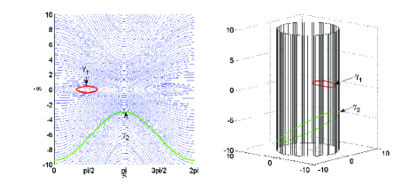
Figure 2. Left: Phase portrait of an EL system. Right: An oscillation ($\gamma_{1}$) and a rotation ($\gamma_{2}$) on the cylinder.

Example 7.2.

For the system

$$\ddot{s}=\cos(s)+0.5+\cos(s)\dot{s}^{2},$$

where $s\in[\mathbb{R}]_{2\pi}$, we have

$$\tilde{M}(x)=\exp\Big{(}-2\int_{0}^{x}\tilde{\Psi}_{2}(\tau)d\tau\Big{)}=\exp\big{(}-2\int_{0}^{x}\cos\tau d\tau\big{)}=\exp(-2\sin x),$$

is $2\pi$-periodic. On the other hand, one can check that $\tilde{V}(2\pi)=-\int_{0}^{2\pi}(\cos\tau+0.5)\exp(-2\sin\tau)d\tau\simeq 7.1615\neq 0$, so that $\tilde{V}$ is not $2\pi$-periodic. By Theorem 3.7, the system is SEL. By Proposition 6.5, almost all its solutions are either oscillations or helices. Figure 3 shows the phase portrait and two typical phase curves on the cylinder, an oscillation and a helix.

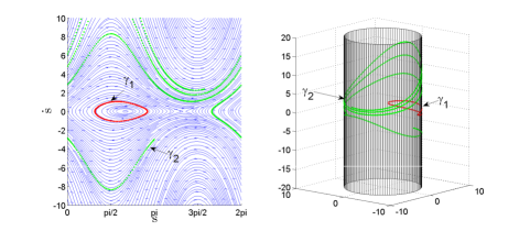
Figure 3. Left: Phase portrait of a SEL system. Right: An oscillation ($\gamma_{1}$) and a helix ($\gamma_{2}$) on the cylinder.

Example 7.3.

For the system $\ddot{s}=\lambda$, with $\lambda\neq 0$ and $s\in[\mathbb{R}]_{T}$, we have $\tilde{M}(x)=1$ and $\tilde{V}(x)=-\lambda x$. Since $\tilde{M}$ is $T$ periodic and $\tilde{V}$ isn’t, the system is SEL. By Theorem 3.7, the Lagrangian is given by (3.3). The Euler-Lagrange equation with this Lagrangian reads

$$\frac{d}{dt}\frac{\partial{\tilde{L}}}{\partial\dot{x}}-\frac{\partial{\tilde{L}}}{\partial x}=\frac{2\pi}{\lambda T}\cos\Big{(}\frac{2\pi}{\lambda T}(\dot{x}^{2}/2-\lambda x)\Big{)}(\ddot{x}-\lambda)=0.$$

We see that all solutions of the system $\ddot{s}=\lambda$ satisfy the Euler-Lagrange equation, but there are signals $(x(t),\dot{x}(t))=(T/4+kT,0)$, $k\in\mathbb{Z}$ satisfying the Euler-Lagrange equation which do not satisfy the equation $\ddot{s}=\lambda$. Thus, the collection of solutions of a SEL system is contained, but is not equal to, the collection of solutions of the associated Euler-Lagrange equation.

Example 7.4.

Consider the system

$$\dot{s}=-\cos(s)-2+(\sin(s)+2)\dot{s}^{2}$$

with $s\in[\mathbb{R}]_{2\pi}$. We have $\Psi_{1}(s)=-\cos(s)-2<0$ and $\int_{0}^{2\pi}\tilde{\Psi}_{2}(\tau)d\tau=\int_{0}^{2\pi}(\sin\tau+2)d\tau=4\pi>0$. This latter identity implies that $\tilde{M}(2\pi)\neq 0$, so that $\tilde{M}$ is not $2\pi$-periodic, and the system is neither EL nor SEL. Moreover, by Proposition 6.7 the system has an exponentially stable limit cycle with domain of attraction including $\mathcal{D}=\{(s,\dot{s})\in T[\mathbb{R}]_{2\pi}:\dot{s}\leq 0\}$. Figure 4 depicts the phase portrait of the system along with the stable limit cycle.

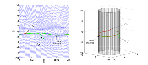
Figure 4. Left: Phase portrait of a non EL system with an attractive limit cycle. Right: Two phase curves and the stable limit cycle of the system on the phase cylinder.

Example 7.5.

We return to the particle mass example of Section 1, in which $s\in[\mathbb{R}]_{2\pi}$ and

$$\Psi_{1}(s)=-\frac{\left(a_{1}b_{2}+a_{2}b_{1}-a_{1}\sin(s)+a_{2}\cos(s)\right)\left(b_{1}\cos(s)+b_{2}\sin(s)+1\right)}{\left[(b_{1}-a_{1}+\cos(s))^{2}+(b_{2}-a_{2}+\sin(s))^{2}\right]^{3/2}}$$

$$\Psi_{2}(s)=-\frac{b_{1}\sin(s)+b_{2}\cos(s)}{b_{1}\cos(s)+b_{2}\sin(s)+1},$$

where $a_{i},b_{i}$ are the components of $a,b\in\mathbb{R}^{2}$. We now revisit the four cases discussed in Section 1.

Case 1: $a=b=0$. In this case the reduced dynamics reads as $\ddot{s}=0$, an EL system.

Case 2: $a=0,b\neq 0$. Here we have $\Psi_{1}=0$, implying that $\tilde{V}$ is $2\pi$-periodic. Moreover, one can check that $\tilde{M}(x)=(4+\cos x)^{2}/25$, a $2\pi$-periodic function. Thus the reduced dynamics are EL. In this case, the Lagrangian function $L(s,\dot{s})=1/2M(s)\dot{s}^{2}$ is not equal to the restriction of the Lagrangian of the particle mass, $\mathcal{L}(q,\dot{q})=(1/2)\|\dot{q}\|^{2}-P(q)$ to the constraint manifold.

Case 3: $a=[1/4\ \ 3/4]^{\top},b=[3/4\ \ 0]^{\top}$. In this case $\Psi_{2}(s)$ is the same as in case 2, but now $\Psi_{1}(s)\neq 0$. While $\tilde{M}$ is $2\pi$-periodic, one can check that $\tilde{V}(2\pi)=0.2762\neq 0$. The virtual potential is not $2\pi$-periodic and thus the system is SEL. Figure 5 shows two typical solutions on the cylinder, an oscillation and a helix.

\psfrag{s}{$s$}\psfrag{t}{$\dot{s}$}\includegraphics[width=411.93767pt]{./phase_portrait_mass.eps}

Figure 5. Left: phase portrait of the particle mass example in case 3. Right: an oscillation and a helix on the phase cylinder.

Case 4: $a=b=0,B(q)=R_{\theta}q$, $\theta\in(-\pi/2,\pi/2)$, $\theta\neq 0$. In this case, the reduced dynamics read as

$$\ddot{s}=\frac{\tan\theta}{5}-(\tan\theta)\ddot{s}^{2}.$$

We have $\tilde{M}(x)=\exp(-2\int_{0}^{x}-\tan(\theta)d\tau)=\exp(2(\tan\theta)x)$. This is not $2\pi$-periodic and thus the reduced dynamics is neither EL nor SEL. In sum, arbitrarily small variations of the parameters $a,b,\theta$ have drastic effects on the Lagrangian properties of the reduced dynamics of the particle.