IPPP/17/36
Multiparticle production in the large $\lambda n$ limit:
Realising Higgsplosion in a scalar QFT

Abstract

In a scalar theory which we use as a simplified model for the Higgs sector, we adopt the semiclassical formalism of Son for computations of $n$-particle production cross-sections in the high-multiplicity $n\to\infty$ weak-coupling $\lambda\to 0$ regime with the value of $\lambda n$ held fixed and large. The approach relies on the use of singular classical solutions to a certain boundary value problem. In the past this formalism has been successfully used and verified in computations of perturbative multi-particle processes at tree-level, and also at the next-to-leading order level in the small $\lambda n$ expansion near the multi-particle mass threshold. We apply this singular solutions formalism in the regime of ultra-high multiplicities where $\lambda n\gg 1$, and compute the leading positive $\sim n\,\sqrt{\lambda n}$ contribution to the exponent of the multi-particle rate in this large $\lambda n$ limit. The computation is carried out near the multi-particle mass threshold where the multiplicity $n$ approaches its maximal value allowed by kinematics. This calculation relies on the idea of Gorsky and Voloshin to use a thin wall approximation for the singular solutions that resemble critical bubbles. This approximation is justified in precisely the high-multiplicity $\sqrt{\lambda n}\to\infty$ regime of interest. Based on our results we show that the scalar theory with a spontaneous symmetry breaking used here as a simplified model for the Higgs sector, is very likely to realise the high-energy Higgsplosion phenomenon.

1 Introduction

The discovery of a light Higgs boson at the Large Hadron Collider [1, 2], taken together with the apparent lack of any evidence for additional beyond the Standard Model degrees of freedom at energies accessible by current experiments, leaves us with a fundamental problem of how to stabilise the Higgs mass. With a safe assumption that the Standard Model does not account for all microscopic interactions in nature and that the more complete theory is likely to include some super-heavy degrees of freedom we are led to the well-known Hierarchy or the fine-tuning problem for the Higgs mass. Quantum corrections to the Higgs mass induced by the scale of new physics in the UV push the Standard Model Higgs boson mass parameter into the UV domain, unless there is an underlying symmetry reason that the quantum effects cancel among each other, or are not present to start with.

One very recent proposal for addressing the Hierarchy problem that does not rely on supersymmetry or Higgs compositeness, is the Higgsplosion mechanism introduced in Ref. [3]. The main idea of the approach is to destroy all the super-heavy states $X$ by allowing them to rapidly decay into multiple Higgs bosons $X\to n\times h$ at energy scales much below their mass $M_{X}$. In other words, one aims to have the multi-particle decay widths $\Gamma_{X\to n\times h}$ to exceed $M_{X}$ at energies $\sqrt{s_{\star}}\ll M_{X}$. In this sense, the heavy $X$ states become unrealised as particle states, they decay faster than they form, and in practical calculations, the loop integrals involving loops of virtual $X$ fields are effectively cut-off at the relatively low scale $\sqrt{s_{\star}}\ll M_{X}$.

The aim of the present article is to show that the Higgsplosion mechanism can be realised in simple quantum field theoretical settings. As in Ref. [3] we will concentrate on a model with a single real scalar degree of freedom $h(x)$,

$${\cal L}\,=\,\frac{1}{2}\,\partial^{\mu}h\,\partial_{\mu}h\,-\,\frac{\lambda}{4}\left(h^{2}-v^{2}\right)^{2}\,.$$ (1.1)

This theory is a reduction of the SM Higgs sector in the unitary gauge to a single scalar field $h(x)$ which for our purposes we take to be stable, so there are no decays into fermions, and we have also decoupled all vector bosons, etc. The vacuum expectation value $v$ results in a spontaneous symmetry breaking of the $h\to-h$ discrete symmetry and the field $\varphi(x)=h(x)-v$ describes the boson of mass $M_{h}=\sqrt{2\lambda}\,v$. From now on we will treat (1.1) as the simplified model description of the self-interacting Higgs sector and will ignore effects of other interactions of the Higgs with the Standard Model vectors and fermions. Clearly the effects of such interactions will ultimately need to be understood and estimated for a more realistic phenomenological treatment. Here we will stick with a simpler goal – which is to demonstrate that the concept of Higgsplosion can be realised in a concrete simple scalar field theory example. In the Discussion section we will briefly comment on the more general cases.

The aim of this paper is to compute the multi-boson production rate in the large $\lambda n$ limit, where $\lambda$ is the coupling constant and $n$ is the particle number in the final state. On the technical side, the idea which makes this calculation possible, is to combine the semiclassical formalism developed by Son in Ref. [4] based on singular classical solutions with the approach of Gorsky and Voloshin [5] which will allow us to search for these solutions in the form of thin walled singular bubbles.

This paper is organised as follows. In section 2, following a brief recollection of known results for multi-particle amplitudes, we will summarise the semiclassical approach of [4] aimed at computing the cross-sections for such processes at very high energies. In section 3 we will continue with this semiclassical technique and will relate it to the problem of finding extrema of Euclidean actions computed on singular surfaces. This problem will be addressed and solved in section 4 using the thin-wall approximation in the large final state multiplicity limit. There we will employ the approach of [5] developed for thin-wall bubbles. Finally, in section 5 we will provide a detailed discussion of the main results, their consequence for the Higgsplosion picture [3] and comments on future directions.

2 Semiclassical approach for multi-particle production

In the scattering processes at very high energies, production of large numbers of particles in the final state becomes possible. We will concentrate on such processes in a scalar field theory. These processes were studied in some detail in the literature and we refer the reader to a selection of papers [6, 7, 8, 9, 10, 11, 12, 13, 14, 5, 4, 15, 16, 17, 18] and references therein.

To start, we consider the leading order tree-level $n$-point scattering amplitude computed on the $n$-particle mass thresholds. This is the kinematics regime where all final state particles are produced at rest. These amplitudes for all $n$ are conveniently assembled into a single object – the amplitude generating function – which at tree-level is described by a particular solution of the Euler-Lagrange equations. The classical solution which provides the generating function of tree-level amplitudes on multi-particle mass thresholds in the model (1.1) is given by [9],

$$h_{\rm cl}(z_{0};t)\,=\,v\,\left(\frac{1+z_{0}\,e^{iM_{h}t}/(2v)}{1-z_{0}\,e^{iM_{h}t}/(2v)}\right)\,,$$ (2.1)

where $z_{0}$ is an auxiliary variable. It is easy to check with the direct substitution that the expression in (2.1) does indeed satisfy the Euler-Lagrange equation resulting from our theory Lagrangian (1.1) for any value of the $z_{0}$ parameter. It then follows that all $1\to n$ tree-level scattering amplitudes on the $n$-particle mass thresholds are given by the differentiation of $h_{\rm cl}(z_{0};t)$ with respect to $z_{0}$,

$${\cal A}_{1\to n}\,=\,\langle n|S\phi(0)|0\rangle\,=\,\,\left.\left(\frac{\partial}{\partial z_{0}}\right)^{n}h_{\rm cl}\,\right|_{z_{0}=0}$$ (2.2)

The classical solution in (2.1) can be thought of as a holomorphic function of the complex variable $z(t)=z_{0}\,e^{iM_{h}t}$,

$$h_{\rm cl}(z(t))\,=\,v\,+\,2v\,\sum_{n=1}^{\infty}\left(\frac{z(t)}{2v}\right)^{n}\,,$$ (2.3)

so that the amplitudes in (2.2) are given by the coefficients of the Taylor expansion in (2.3) times $n!$ from differentiating $n$ times over $z$,

$${\cal A}_{1\to n}\,=\,\left.\left(\frac{\partial}{\partial z}\right)^{n}h_{\rm cl}\,\right|_{z=0}\,=\,n!\,\left(\frac{1}{2v}\right)^{{n-1}}\,,$$ (2.4)

These formulae and the characteristic factorial growth of $n$-particle amplitudes, ${\cal A}_{n}\sim\lambda^{n/2}n!$, form the essence of the elegant formalism pioneered by Brown in Ref. [9] that is based on solving classical equations of motion and bypasses the summation over individual Feynman diagrams. For more detail and derivations we refer the reader to the original paper [9] or a review in Section 2 of Ref. [19].

We now perform the Wick rotation from the real Minkowski time $t$ to the Euclidean time $t_{\rm Eucl}=it$. To use the same notation for the imaginary time variable as in [4] we will use the variable $\tau$ defined as,

$$\tau\,:=\,-\,t_{\rm Eucl}\,=\,-\,it\,.$$ (2.5)

Expressed as the function of the Wick-rotated time variable $\tau$, the classical solution (2.1) reads,

$$h_{\rm cl}(\tau)\,=\,v\,\left(\frac{1\,+\,e^{-M_{h}(\tau-\tau_{\infty})}}{1\,-\,e^{-M_{h}(\tau-\tau_{\infty})}}\right)\,,$$ (2.6)

where the $\tau_{\infty}$ parameter, $\tau_{\infty}=\frac{1}{M_{h}}\log\left(\frac{z_{0}}{2v}\right)$, gives the location of the solution in time. The sign convention in (2.5) where $\tau$ is identified with the negative of the Euclidean time, implies that the early time $t\to-\infty$ corresponding to the initial time, i.e. the incoming states, maps to $\tau\to+\infty$. In this limit the classical solution approaches the vacuum $h_{\rm cl}\to v$ with exponential accuracy, i.e. the corrections are ${\cal O}(e^{-M_{h}\tau})$.

The expression on the right hand side of (2.6) has an obvious interpretation in terms of a singular domain wall located at $\tau=\tau_{\infty}$ that separates two domains of the field $h(\tau,\vec{x})$. The domain on the right of the wall $\tau\gg\tau_{\infty}$ has $h\sim+v$, and the domain on the left of the wall, $\tau\ll\tau_{\infty}$, is characterised by $h\sim-v$. The field configuration is singular at the position of the wall, $\tau=\tau_{\infty}$, for all values of $\vec{x}$, i.e. the singularity surface is flat (or uniform in space). The thickness of the wall is set by $1/M_{h}$.

In Ref. [4] Son proposed a semiclassical approach for computing multi-particle cross-sections in a scalar QFT. This approach is quite general, as it works not only for the leading-order tree-level processes, but is also capable of computing the higher-order quantum loop-level effects. Furthermore the method is designed to provide probabilistic quantities, i.e. the rates or cross-sections, hence it goes beyond just the calculation of the amplitudes near or on the mass-thresholds by also taking account of the integrations over the $n$-particle Lorentz-invariant phase space. The approach of [4] generalised to field theory the Landau WKB method [20] for computing matrix elements of certain generic local operators between the initial and final states with different energy eigenvalues. In our case, the initial state is a vacuum and the final state is the $n$-particle final state with $n\gg 1$. It is known that to the leading exponential accuracy the transition rates computed using the Landau WKB method do not depend on the specific form of the operator ${\cal O}(x)$ used to deform the initial state, if this deformation is not exponential. It is then similarly expected that the choice of the operator does not affect the transition rates in the QFT settings either, and the approach of [4] generalises the Landau WKB method to a scalar QFT using the path integral formalism.

The central quantity is the dimensionless probability rate ${\cal R}_{n}(E)$ for a local operator ${\cal O}$ to create $n$ particles of total energy $E$ from the vacuum. It is given by [4],

$${\cal R}_{n}(E)\,=\,\int d\Phi_{n}\,\langle 0|\,{\cal O}^{\dagger}\,S^{\dagger}\,P_{E}|n\rangle\langle n|\,P_{E}\,S\,{\cal O}\,|0\rangle\,,$$ (2.7)

where the matrix element involves the operator ${\cal O}$ between the vacuum state $|0\rangle$ and the $n$-particle state of fixed energy $\langle n|\,P_{E}$ (here $P_{E}$ is the projection operator on states with fixed energy $E$), along with the $S$ matrix to evolve between the initial and finial times. The matrix element is squared and integrated over the $n$-particle Lorentz-invariant phase space $\Phi_{n}$

$$\int d\Phi_{n}\,=\,\frac{1}{n!}\,(2\pi)^{4}\delta^{(4)}(P_{\rm in}-\sum_{j=1}^{n}p_{j})\,\prod_{j=1}^{n}\int\frac{d^{3}p_{j}}{(2\pi)^{3}\,2p_{j}^{0}}\,.$$ (2.8)

Note that in our conventions the bosonic phase-space volume element (2.8) includes the $1/n!$ symmetry factor for the production of the $n$ equivalent Higgs bosons.

The local operator ${\cal O}$ appearing in the matrix elements in (2.7) is usually chosen to be [4]

$${\cal O}\,=\,{e^{j\,(h(0)-v)}}:=e^{j\phi(0)}\,,$$ (2.9)

where $j$ is a constant, and the limit $j\to 0$ is taken in the computation of the probability rates,

$${\cal R}_{n}(E)\,=\,\lim_{j\to 0}\int d\Phi_{n}\,\langle 0|\,{e^{j\phi(0)}}^{\dagger}\,S^{\dagger}\,P_{E}|n\rangle\langle n|\,P_{E}\,S\,{e^{j\phi(0)}}\,|0\rangle\,.$$ (2.10)

The cross-sections for few to many particles, $\sigma_{{\rm few}\to n}(E)$ as well as multi-particle partial decay rates $\Gamma_{n}(E)$ of a single particle state $X\to n\times h$, are determined by the exponential factor for ${\cal R}_{n}(E)$ in (2.10) times a non-exponential pre-factor of appropriate dimensionality which is of no interest in a semiclassical approximation.

In the construction of [4] the expression on the right hand side of (2.10) is represented as a functional integral, which is subsequently computed in the steepest descent approximation for all integration variables. This is achieved and justified in the double-scaling weak-coupling / large-$n$ semiclassical limit:

$$\lambda\to 0\,,\quad n\to\infty\,,\quad{\rm with}\quad\lambda n={\rm fixed}\,,\quad\varepsilon={\rm fixed}\,.$$ (2.11)

Here $\varepsilon$ denotes the average kinetic energy per particle per mass in the final state,

$$\varepsilon\,=\,(E-nM_{h})/(nM_{h})\,.$$ (2.12)

Holding $\varepsilon$ fixed implies that in the large-$n$ limit we are raising the total energy linearly with $n$.

The semiclassical result for the rate has the characteristic exponential form [4],

$${\cal R}_{n}(E)\,\simeq\,\exp\left[W(E,n)\right],$$ (2.13)

where

$$W(E,n)\,=\,\frac{1}{\lambda}\,{\cal F}(\lambda n,\varepsilon)\,=\,ET\,-\,n\theta\,-\,2{\rm Im}S[h]\,.$$ (2.14)

Let us now examine the structure of this result. The function ${\cal F}(\lambda n,\varepsilon)$ appearing in (2.14), is a function of two finite-valued arguments while all the integrations in the path integral representation of ${\cal R}_{n}(E)$ in (2.10) were carried out and saturated by their saddle-point values in the large-$n$, large-$1/\lambda$ limit (2.11). At negative values of ${\cal F}(\lambda n,\varepsilon)$ the multi-particle rate ${\cal R}_{n}(E)$ is exponentially suppressed, while if ${\cal F}(\lambda n,\varepsilon)$ crosses zero and becomes positive above some critical energy or multiplicity, the multi-particle processes enter the Higgsplosion phase [3].

We now consider the terms appearing in the final expression in (2.14). First, the combination $-\,2{\rm Im}S[h]$ follows from the $e^{-iS[h]^{*}}e^{iS[h]}$ factor in the product of the matrix elements in (2.10). The integration contours and the resulting saddle-points in the steepest descent integration are complex-valued, hence $iS[h]-iS[h]^{*}\,=\,-\,2{\rm Im}S[h]$ or equivalently $-2S_{\rm Eucl}[h]$ using the Euclidean notation. Finally, the parameters $T$ and $\theta$ appearing on the right hand side of (2.14) are the consequence of introducing projections onto the final states with defined values of the energy $E$ and the particle number $n$ in (2.10).

The function $W(E,n)$ in (2.13)-(2.14) is computed on the saddle-point value of the path integral. Prior to taking the $j\to 0$ limit in (2.10), the saddle-point field configuration $h(x)$ is given by a particular solution to the classical equation of motion with the singular source term $j(x)=\,j\delta^{(4)}(x)$ on the right hand side,

$$\frac{\delta S}{\delta h(x)}\,=\,i\,j\,\delta^{(4)}(x)\,,$$ (2.15)

where $S=\int d^{4}x{\cal L}$ is the action of the theory and $j$ is a constant. After taking the limit $j\to 0$, the right hand side of the defining equation (2.15) vanishes but the required solution nevertheless remains singular at $x=0$ in Minkowski space. The saddle-point solution also depends on the parameters $T$ and $\theta$, as will be explained below, while the overall expression $W(E,n)$ is independent of $T$ and $\theta$. Hence,

$$2\,\frac{\partial\,{\rm Im}S}{\partial T}\,=\,E\,,\qquad 2\,\frac{\partial\,{\rm Im}S}{\partial\theta}\,=\,-\,n\,,$$ (2.16)

and $W(E,n)$ is the Legendre transformation of the action $2{\rm Im}S$ with respect to $T$ and $\theta$.

Next step is to specify the boundary conditions of the solution $h(x)$ at $t_{\rm in}\to-\infty$ and $t_{\rm fin}\to+\infty$. At the initial and final time boundaries $h(x)$ satisfies the free Klein-Gordon equation, thus

$$h(\vec{x},t)|_{t\to-\infty} \to v\,+\,\int\frac{d^{3}k}{(2\pi)^{3/2}}\frac{1}{\sqrt{2\omega_{\bf k}}}\,\,a^{\dagger}_{\bf k}\,e^{ik_{\mu}x^{\mu}}\,$$ (2.17)

$$h(\vec{x},t)|_{t\to+\infty} \to v\,+\,\int\frac{d^{3}k}{(2\pi)^{3/2}}\frac{1}{\sqrt{2\omega_{\bf k}}}\left(c_{\bf k}\,e^{-ik_{\mu}x^{\mu}}\,+\,b^{\dagger}_{\bf k}\,e^{ik_{\mu}x^{\mu}}\right)\,.$$ (2.18)

where we used the standard notation $k_{0}=\omega_{\bf k}=\sqrt{M_{h}^{2}+{\bf k}^{2}}$ so that $e^{\pm ik_{\mu}x^{\mu}}=e^{\pm i(\omega_{\bf k}t\,-\,{\bf k}{\bf x})}$.
The $t\to-\infty$ boundary condition in Eq. (2.17) contains only the positive frequency components $\frac{1}{\sqrt{2\omega_{\bf k}}}\,a^{\dagger}_{\bf k}\,e^{-i\omega_{\bf k}|t|}$ and no negative frequency ones $\frac{1}{\sqrt{2\omega_{\bf k}}}\,a_{\bf k}\,e^{+i\omega_{\bf k}|t|}$. In the second quantisation operator formalism, this condition implements the requirement that there are no particles in the initial state, $\langle 0|\,\int\frac{1}{\sqrt{2\omega_{\bf k}}}\,a^{\dagger}_{\bf k}\,e^{-i\omega_{\bf k}|t|}\,=\,0$ since the creation operator $a^{\dagger}$ annihilates the bra-state vacuum $\langle 0|.$ The second boundary condition (2.18) at the final time $t\to+\infty$ contains both positive and negative frequency components. Following [4] we parameterise its $c_{\bf k}$ coefficient in terms of the complex conjugate of its $b_{\bf k}^{\dagger}$ coefficient,

$$c_{\bf k}\,=\,b_{\bf k}\,e^{\omega_{\bf k}T-\theta}\,.$$ (2.19)

The solution is complex-valued since $c_{\bf k}\neq\,b_{\bf k}$, and the corresponding parameters $T$ and $\theta$ are precisely those appearing in (2.16).

In summary, the equations (2.15)-(2.19) specify the boundary value problem for finding the saddle-point configuration $\{h(x),T,\theta\}$ needed to compute the semiclassical rate ${\cal R}_{n}(E)$:

1. Solve the classical equation without the source-term,

   $$\frac{\delta S}{\delta h(x)}\,=\,0\,,$$

   by finding a complex-valued solution $h(x)$ with a point-like singularity at the origin $x^{\mu}=0$ and regular everywhere else in Minkowski space.

2. Impose the initial and final-time boundary conditions,

   $$\lim_{t\to-\infty}\,h(x) = v\,+\,\int\frac{d^{3}k}{(2\pi)^{3/2}}\frac{1}{\sqrt{2\omega_{\bf k}}}\,\,a^{\dagger}_{\bf k}\,e^{ik_{\mu}x^{\mu}}\,$$

   $$\lim_{t\to+\infty}\,h(x) = v\,+\,\int\frac{d^{3}k}{(2\pi)^{3/2}}\frac{1}{\sqrt{2\omega_{\bf k}}}\left(b_{\bf k}\,e^{\omega_{\bf k}T-\theta}\,e^{-ik_{\mu}x^{\mu}}\,+\,b^{\dagger}_{\bf k}\,e^{ik_{\mu}x^{\mu}}\right)\,.$$

3. Compute the energy and the particle number using the $t\to+\infty$ asymptotics of $h(x)$,

   $$E\,=\,\int d^{3}k\,\,\omega_{\bf k}\,b_{\bf k}^{\dagger}\,b_{\bf k}\,e^{\omega_{\bf k}T-\theta}\,,\qquad n\,=\,\int d^{3}k\,\,b_{\bf k}^{\dagger}\,b_{\bf k}\,e^{\omega_{\bf k}T-\theta}\,.$$

   At $t\to-\infty$ the energy and the particle number are vanishing. The energy is conserved by regular solutions and changes discontinuously from $0$ to $E$ at the singularity at $t=0$.

4. Eliminate the $T$ and $\theta$ parameters in favour of $E$ and $n$ using the expressions above. Finally, compute the function $W(E,n)$

   $$W(E,n)\,=\,ET\,-\,n\theta\,-\,2{\rm Im}S[h]$$

   on the set $\{h(x),T,\theta\}$, and thus determine the semiclassical rate ${\cal R}_{n}(E)\,=\,\exp\left[W(E,n)\right]$.

3 Solving the boundary-value problem by extremizing the
Euclidean action over the singular surfaces

One way to visualise the construction of the solution to the boundary-value problem outlined above, is by starting with the specified expressions for $h(x)$ at the $t\to\pm\infty$ boundaries and classically evolving them by numerically solving the equation of motion into the region of finite $t$. We thus have two trial functions, one at $t<0$ and the second at $t>0$ which we would like to match at $t=0$. The field configuration at $t<0$ is given by a regular classical solution $h_{1}(t,\vec{x})$ which satisfies the initial time boundary condition with the Fourier coefficient functions $a_{\bf k}$. The second trial function, $h_{2}(t,\vec{x})$, is a regular classical solution on the Minkowski half-plane $t>0$ which is evolved from the final-time boundary condition with the coefficient functions $b_{\bf k}$. One then contemplates scanning over the space of the functions $a_{\bf k}$ and $b_{\bf k}$ to achieve the matching at $t=0$ between the two branches $h_{1}$ and $h_{2}$ of the solution, $h_{1}(\vec{x})=h_{2}(\vec{x})$, and all of its time derivatives for all values of $\vec{x}\neq 0$. The only allowed singularity of the full solution is point-like, and located at the origin $t=0=\vec{x}$.

As was pointed out in [4], the construction of the saddle-point solution above has a more natural implementation in terms of the complex-valued time coordinate. In Minkowski space-time $x^{\mu}=(t,\vec{x})$ the solution $h(x)$ contains a point-like singularity at the origin $x=0$ arising from the delta-function source term in (2.15), and is regular everywhere else. In the Euclidean space-time, $(\tau,\vec{x})$, however, the solution will in general be singular on a hypersurface $\tau=\tau_{0}(\vec{x})$. For a particularly simple case of the uniform in space solution (2.6), the singularity surface is $\tau_{0}=\tau_{\infty}$ which is an $\vec{x}$-independent constant as we have already seen. This solution describes the generating functional of tree-level amplitudes on $n$-particle mass thresholds. In the more non-trivial settings, specifically in the case of solutions relevant for the processes away from the multi-particle thresholds, or beyond the tree-level, or both, the relevant fields do depend on the spacial variable and as the result, the singularity surface $\tau=\tau_{0}(\vec{x})$ is an ${\cal O}(3)$ symmetric function of the spacial variable. Consider the singularity surface $\tau_{0}(\vec{x})$ of the form shown in the Figure (1a). It is a local deformation of the flat singularity domain wall at $\tau_{\infty}$ with the single maximum touching the origin $(\tau,\vec{x})=0$. As such, in Minkowski space the singularity is point-like at $t=i\tau=0$ and $\vec{x}=0$ as required.

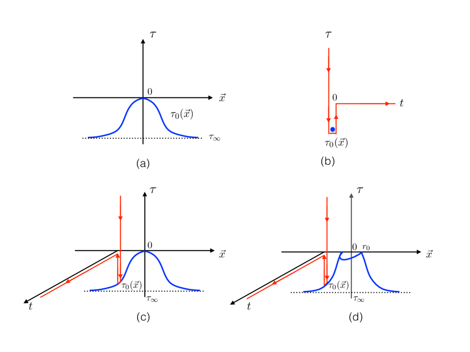
Figure 1: Figure (1a) shows the singularity surface $\tau=\tau_{0}(\vec{x})$ of the field configuration $h$ on the imaginary-time hyper-plane $(\tau,\vec{x})$. The tip of the singularity surface is located at $\tau=0$ so that in Minkowski space-time the solution is singular only at a single point taken to be the origin $(t,\vec{x})=(0,\vec{0})$. Away from the local maximum, the singular domain-wall $\tau_{0}(\vec{x})$ approaches the constant space-independent value $\tau_{\infty}$. Figure (1b) shows the time-evolution contour on the complex time plane. The two turning points are the location of the singularity surface, $\tau_{0}(\vec{x})$, and the origin, $\tau=0=t$, after which evolution to the final state proceeds along the real $t$ axis. Figure (1c) shows the same time-evolution contour at a fixed value of $\vec{x}$ along with the singularity surface of the classical field in the complex-time–space coordinate system $(t,\tau,\vec{x})$. Figure (1d) is the same as (c), but the singular domain wall $\tau_{0}(\vec{x})$ is folded into the real time direction for $|x|<r_{0}$ where $r_{0}$ is the critical radius of the domain wall bubble.

Thus by extending the real time variable into the complex plane we have extended the point-like singularity of the solution to the singularity hypersurface $\tau=\tau_{0}(\vec{x})$ or the singular domain wall. The next step is to define the time evolution contour of the solution in the complex plane from the initial to the final time boundaries. It is shown in the Figure (1b). At early times the solution evolves along the imaginary-time axis from the initial time boundary at $\tau=+\infty$ down to the singularity surface of the solution at $\tau_{0}$. The contour then encircles the singularity $\tau_{0}$ at each fixed value of $\vec{x}$ and evolves upwards along the imaginary-time axis to $\tau=0$. From there on the third segment the contour evolves along the real-time axis from $t=0$ to the final-time boundary at $t\to+\infty$. The Figure (1c) shows this contour in the $(t,\tau,\vec{x})$ coordinates along with the singularity surface of the solution at $\tau=\tau_{0}(\vec{x})$.

We now return to the two branches of the solution $h_{1}(\tau,\vec{x})$ and $h_{2}(t,\vec{x})$ introduced in the beginning of this section, but now defined along the time evolution contour in Fig. 1. Both these field configurations are finite regular classical solutions on the subspaces defined by $\tau>\tau_{0}(\vec{x})$ for $h_{1}(\tau,\vec{x})$, and by $t>0$ for $h_{2}(t,\vec{x})$. They satisfy the boundary conditions (cf. (2.17)-(2.18) and recall the substitution $t=i\tau$ for the initial time asymptotics),

$$\lim_{\tau\to+\infty}\,h_{1}(\tau,\vec{x})\,-\,v = 0\,$$ (3.1)

$$\lim_{t\to+\infty}\,h_{2}(t,\vec{x})\,-\,v = \int\frac{d^{3}k}{(2\pi)^{3/2}}\frac{1}{\sqrt{2\omega_{\bf k}}}\left(b_{\bf k}\,e^{\omega_{\bf k}T-\theta}\,e^{-ik_{\mu}x^{\mu}}\,+\,b^{\dagger}_{\bf k}\,e^{ik_{\mu}x^{\mu}}\right)\,.$$ (3.2)

The Euclidean action of the complete solution $h(x)$ along our complex-time contour can be straightforwardly represented as the appropriate action integrals of the solutions $h_{1}(\tau,\vec{x})$ and $h_{2}(t,\vec{x})$ on the parts of the contour,

$$S_{\rm Eucl}\,=\,\int d^{3}x\left[-\int_{+\infty}^{\tau_{0}(\vec{x})}d\tau\,{\cal L}_{\rm Eucl}(h_{1})\,-\,\int_{\tau_{0}(\vec{x})}^{0}d\tau\,{\cal L}_{\rm Eucl}(h_{2})\,-\,i\int_{0}^{\infty}dt\,{\cal L}(h_{2})\right]\,,$$ (3.3)

where we used the standard notation ${\cal L}_{\rm Eucl}(h)\,=\,\frac{1}{2}\left(\partial_{\mu}h\right)^{2}\,+\,V(h)$, $S_{\rm Eucl}\,=\,-i\,S$ and recalled that $\tau=-t_{\rm Eucl}$ (which explains the minus signs in the first two terms).

Up to this point we have not attempted to impose any matching conditions on the two trial functions, $h_{1}(\tau,\vec{x})$ and $h_{2}(\tau,\vec{x})$, at the singularity. Without the matching, the two individual components are some easy-to-obtain classical solutions with the correct boundary conditions at the initial $\tau\to\infty$ and final $t\to\infty$ times, but they do not solve the required boundary value problem. First one can imagine adjusting the coefficients $b_{\bf k}$ to match the two profiles on a certain candidate surface $A$, so we set $h_{1}\,=\,h_{2}\,=\,\Phi_{0}$ on $A$. We assume a regularisation procedure which keeps $\Phi_{0}$ finite at intermediate stages of the calculation to avoid infinities. The approximation to the true saddle-point is still very crude as the derivatives normal to the surface do not match, and the matching of $h_{1}$ and $h_{2}$ has a cusp on the entire surface $A$,

$$\partial_{n}(h_{1}\,-\,h_{2})\,=\,J(A)\,.$$ (3.4)

This defines a function $J(A)$ supported on the surface of $A$. It then follows that the field configuration $h(x)$ obtained from this matching satisfies the equation

$$\frac{\partial S_{\rm Eucl}}{\partial h}\,=\,J(x)\,,\quad{\rm where}\quad J(x)\,=\,\int d^{3}A\,J(A)\,\delta^{(4)}(x-x(A))\,.$$ (3.5)

This is the classical equation with a source $J(x)$ rather than $j\delta^{(4)}(x)$ appearing in the equation (2.15) we are meant to be solving. The important point emphasised in [4] is that we can repair this by varying the shape of the candidate surface $A$, and consider a family of Euclidean actions of the form (3.3) each computed using a particular surface $A$. Then it is easy to show that once the action $S_{\rm Eucl}[h]$ has been extremized with respect to $A$, the source $J(x)$ corresponding to the extremal surface becomes of the required $\delta$-function form, $j\delta^{(4)}(x)$.

This concludes our review of the semiclassical method of Son [4]. To summarise our main conclusion in this section, it was shown that the required saddle-point solution to the multi-particle boundary-value problem can be obtained by extremizing the real part of the Euclidean action over all singularity surfaces $\tau=\tau_{0}(\vec{x})$ containing the point $t=0=\vec{x}$.

There are two equivalent formulations of the problem. One either finds the required solution with the point-like singularity at the origin by varying the Fourier coefficients of the solution asymptotics at $t\to\pm\infty$, or alternatively, one extremizes the classical action by varying the singularity surfaces of the solutions in complex time. The second method will be particularly well suited for using the thin-wall approximation in the following section. This will allow us to compute the dominant contribution to $W(E,n)$ in the limit $\lambda n\to\infty.$

4 Thin wall critical bubbles

The main goal of this section is to use the semiclassical method described above to carry out a novel computation of the multi-particle rates ${\cal R}_{n}(E)=\,e^{W(E,n)}$ in the large $\lambda n$ limit. This involves the higher-loop quantum effects, and in order to correctly address them we first need to normalise on the known tree-level high multiplicity results. Our starting point is the function $W$ in (4.1) appearing in the exponent of the rate which is evaluated on the saddle-point solution. In terms of the Euclidean action it is given by,

$$W(E,n;\lambda)\,=\,\frac{1}{\lambda}\,{\cal F}(\lambda n,\varepsilon)\,=\,ET\,-\,n\theta\,-\,2S_{\rm Eucl}[h]\,.$$ (4.1)

At tree-level, the function $W$ is of the form,

$$W(E,n;\lambda)^{\rm tree}\,=\,\frac{\lambda n}{\lambda}\left(f_{0}(\lambda n)\,+\,f(\varepsilon)\right)\,,$$ (4.2)

and its dependence on $\lambda n$ and on the average kinetic anergy per particle per mass, $\varepsilon$, is in terms of two individual functions of each argument, $f_{0}(\lambda n)$ and $f(\varepsilon)$. These functions are known,

$$f_{0}(\lambda n) = \log\left(\frac{\lambda n}{4}\right)-1\,,$$ (4.3)

$$f(\varepsilon)|_{\varepsilon\to 0} \to f(\varepsilon)_{\rm asympt}\,=\,\frac{3}{2}\left(\log\left(\frac{\varepsilon}{3\pi}\right)+1\right)-\frac{25}{12}\,\varepsilon\,,$$ (4.4)

where the expression (4.4) is valid in the non-relativistic limit $\varepsilon\ll 1$ near the multi-particle mass-threshold. These tree-level results (4.2)-(4.4) were computed using both types of methods: the resummation of Feynman diagrams based on solving the recursion relations and integrating over the phase-space in [14, 16], and also from using the semiclassical approach [4] directly. The apparent agreement between the two methods provides a useful consistency check on the semiclassical formalism.

The above result has also been generalised to the general tree-level kinematics. In particular, at tree-level the function $f_{0}(\lambda n)$ is fully determined, but the second function, $f(\varepsilon)$, characterising the energy-dependence of the final state, is determined by Eq. (4.4) only at small $\varepsilon$, i.e. near the multi-particle threshold. This point was addressed in Ref. [18] where the function $f(\varepsilon)$ was computed numerically in the entire range $0\leq\varepsilon<\infty$.

It is also known how to add the leading-order loop corrections to the tree level expressions in the $\lambda n\ll 1$ limit. This has been achieved in Ref. [14] by resumming the one-loop correction to the amplitude on the multi-particle mass threshold originally computed in Refs. [12, 13]. The same result was also reproduced using the semiclassical method [4], once again providing a valuable justification of this approach. This results in the modified expression for $f_{0}$,

$$f_{0}(\lambda n)^{\rm 1-loop}\,=\,\log\left(\frac{\lambda n}{4}\right)-1\,+\,\sqrt{3}\,\frac{\lambda n}{4\pi}\,.$$ (4.5)

To determine whether the bare multi-particle rate ${\cal R}_{n}(E)$ defined in (2.7) and (2.13) can become exponentially large above a certain critical particle number $n$ and lead to a realisation Higgsplosion [3] in a given theory, we need to be able to address the large $\lambda n$ limit. Up to now the loop effects were only computed in the opposite regime of small $\lambda n$ in (4.5).

In the following we will address the large-$n$ limit with the value of the combination $\lambda n$ taken to be large, $\lambda n\gg 1$, while the average particle energy is kept non-relativistic, $\varepsilon\ll 1$. This selects the regime of multiplicities $n$ approaching their maximal values allowed by the fixed energy kinematics, $n\sim n_{\rm max}=E/M_{h}$ where $\varepsilon\sim 0$ and the final state particles are non-relativistic.

The tree-level result (4.2)-(4.4) in the non-relativistic limit $\varepsilon\to 0$ arises in the semiclassical calculation from the uniform in space saddle-point solution (2.6). As we have already discussed, this solution corresponds to a singular domain wall located at a constant value of $\tau$, so that the singularity surface does not depend on $\vec{x}$. In the large $\lambda n$ limit one should be able to similarly write down a singular field configuration that serves as the saddle-point of the path integral representation of the multi-particle rate ${\cal R}_{n}$. The singularity surface of this configuration is however locally deformed by the source at $x=0$, while at large values of $|\vec{x}|$ the singularity surface $\tau_{0}(\vec{x})$ rapidly approaches the constant value $\tau_{0}(\vec{x})\to\tau_{\infty}$.

In both of these cases we need to fix the translational symmetry of the solutions by locating the singularity surfaces in such a way that its local maximum is at the point $\tau=0=\vec{x}$. This implies that the flat domain wall used for calculating the tree-level amplitudes on $n$-particle thresholds should be located at $\tau=0$. At the same time, the $n$-particle amplitudes in the large $\lambda n$ limit arise from the feld configuration with the singularity surface located at $\tau_{0}(\vec{x})$, as described above. Each of these amplitudes are determined by the $z(\tau)^{n}\sim e^{-nM_{h}\tau}$ term in the corresponding Taylor expansion of the field configurations, as in (2.3). Now the difference between the singularity surface located at $\tau=0$ and at $\tau=\tau_{0}(\vec{x})\to\tau_{\infty}$ rescales the ${\cal A}_{1\to n}$ amplitude on the $n$-particle threshold by a multiplicative factor of $e^{-nM_{h}\tau_{\infty}}$.

This is not all. We still need to determine the shape of the curved singularity surface $\tau=\tau_{0}(\vec{x})$ by requiring that it extremizes the Euclidean action on the corresponding singular solution, as was discussed in the previous section. Hence we need to add to the exponent of the rate the factor $-\,2S_{\rm Eucl}[\tau_{0}(x)]\,+\,2S_{\rm Eucl}[0]$ where the last term removes the contribution of the flat wall (already accounted in the tree-level result). These simple qualitative arguments lead to the following form of the $W$ function in the large $\lambda n$ limit (note the factors of 2 arising from squaring the amplitudes),

$$W(E,n;\lambda)\,=\,W(E,n;\lambda)^{\rm tree}\,-\,2nM_{h}\tau_{\infty}\,-\,\left(2S_{\rm Eucl}[\tau_{0}(x)]-\,2S_{\rm Eucl}[0]\right)\,,$$ (4.6)

where by $S_{\rm Eucl}$ we mean the Real part of the Euclidean action (or equivalently the Imaginary part of the Minkowski action). The expression (4.6) is supposed to be valid in the double-scaling large-$n$ limit (2.11) where the two scaling quantities $\lambda n$ and $\varepsilon$ are such that $\lambda n\gg 1$ and $\varepsilon\ll 1.$ The singularity surface $\tau_{0}(x)$, its asymptotics $\tau_{\infty}$ and the Euclidean action itself will now need to be determined as functions of $\lambda$, $\lambda n$ and $\varepsilon$ by extremizing $S_{\rm Eucl}$ as the functional of $\tau_{0}(x)$.

Before we proceed with finding the saddle-point singularity surface for the action, it is worthwhile to note that the same conclusion was also derived in the Section 4.1 of Ref. [4] using a more technical direct approach based on solving the boundary-value problem using a deformation of the flat-wall solution in the form

$$h(\tau,\vec{x})\,=\,v\,\left(\frac{1\,+\,e^{-M_{h}(\tau-\tau_{\infty})}}{1\,-\,e^{-M_{h}(\tau-\tau_{\infty})}}\right)\,+\,\delta h(\tau,\vec{x})$$ (4.7)

with the support on the singular surface $\tau=\tau_{0}(x)$.

The problem of finding the large-$\lambda n$ correction $\frac{1}{\lambda}\,g(\lambda n)$ to the $W$ function has a simple geometric interpretation. We need to maximise the expression

$$\frac{1}{2\lambda}\,g(\lambda n) = -nM_{h}\tau_{\infty}\,-\,{\rm Re}(S_{\rm Eucl}[\tau_{0}(x)]-S_{\rm Eucl}[0])$$ (4.8)

$$= nM_{h}|\tau_{\infty}|\,-\,{\rm Re}(S_{\rm Eucl}[\tau_{0}(x)]-S_{\rm Eucl}[0])\,,$$

where we have used the fact that $\tau_{\infty}$ is negative and hence the first term on the right hand side of (4.8) is positive-valued. This extremization problem corresponds to finding the shape of the membrane with the surface tension dictated by the action $S_{\rm Eucl}$ and located at the position $\tau_{\infty}$ which is pulled at its centre by a constant force.

The main idea on which our calculation will be based is the geometrical interpretation of the saddle-point field configuration as a domain wall solution separating the vacua with different VEVs $h\to\pm v$ on the different sides of the wall. Our scalar theory with the spontaneous symmetry breaking in (1.1) clearly supports such field configurations. The solution is singular on the surface of the wall, and the wall thickness is $\sim 1/M_{h}$. The effect of the ‘force’ $nM_{h}$ applied to the domain wall locally pulls upwards the centre of the wall and gives it a profile $\tau_{0}(\vec{x})$ depicted in Fig. 1. To find the equilibrium position of the domain wall one needs to find an extremum of the expression in (4.8). When computing the Euclidean action on the solution characterised by the domain wall at $\tau_{0}(\vec{x})$, it will be represented by the action of a thin-wall bubble. The shape of the bubble will be straightforward to determine by extremizing the action in the thin-wall approximation, and the validity of this approximation will be shown to be justified in the limit $\lambda n\to\infty$. Our implementation of this set-up will follow closely the construction of Gorsky and Voloshin in Ref. [5].

The Euclidean action computed along the complex time evolution contour shown in Figure (1b) is given by the sum of three contributions, each of them corresponding to one of the three segments of the integration contour. This structure $S_{\rm Eucl}=S_{\rm Eucl}^{(I)}+S_{\rm Eucl}^{(II)}-iS^{(III)}$ is manifest in the expression on the right hand side of (3.3). But only the first two segments contribute to the Real part of $S_{\rm Eucl}$ appearing in the rate in (4.8).

The real part of the action (3.3) computed on the field $h(x)$ which is characterised by the surface of singularities $\tau=\tau_{0}(\vec{x})$ can be written as an integral on the singularity surface in the thin-wall approximation. This is equivalent to stating that the action is equal to the surface tension of the domain wall $\mu$ times the area $A$. We have,

$$S_{\rm Eucl}[\tau_{0}(\vec{x})]\,=\,\int_{\tau_{\infty}}^{0}d\tau\,L(r,\dot{r})\,=\,\int_{\tau_{\infty}}^{0}d\tau\,4\pi\mu\,r^{2}\sqrt{1+\dot{r}^{2}}\,,$$ (4.9)

where $r=|\vec{x}|$ and $\dot{r}=dr/d\tau$. The integral depends on the choice of the domain wall surface $\tau_{0}(\vec{x})$ implicitly via dependence on $\tau$ of $r(\tau)$ and $\dot{r}(\tau)$ which are computed on the domain wall. For the surface tension we have [5],

$$\mu\,=\,\int_{-\infty}^{\infty}d\tau\left(\frac{1}{2}\left(\frac{dh_{\rm cl}}{d\tau}\right)^{2}\,+\,\frac{\lambda}{4}\left(h_{\rm cl}^{2}-v^{2}\right)^{2}\right)\,=\,\frac{M_{h}^{3}}{3\lambda}\,$$ (4.10)

where integral in (4.10) is computed on the flat domain wall solution (2.6),

$$h_{\rm cl}(\tau)\,=\,v\,\left(\frac{1\,+\,e^{-M_{h}(\tau-\tau_{\infty})}}{1\,-\,e^{-M_{h}(\tau+\tau_{\infty})}}\right)$$ (4.11)

with the argument $\tau$ in the equation above further shifted by $i\theta$ with a constant real-valued parameter $\theta$. The physical reason for this shift is that, as we will see below, the singular domain wall will be folded into the real-time direction for $x$ less than the critical radius $r_{0}$ of the bubble as indicated in Fig. (1d). Hence the integration contour along the $\tau$-direction is actually sifted along the real $t$ axis. This also ensures that the integration contour in (4.10) is shifted away from the pole of (4.11) at $\tau=0$. The field configuration in (4.11) is periodic with the period $2i\pi/M_{h}$, and the poles are located at $M_{h}(\tau-\tau_{\infty})=0,\pm 2i\pi,\pm 4i\pi,$ etc. It is easy to see (by closing the integration contour into a loop that does not surround any poles in $\tau$) that any non-vanishing value of $\theta$ in the range $0<M_{h}\theta<2\pi$ would give the same expression $\frac{M_{h}^{3}}{3\lambda}$ for the integral (4.10). For simplicity we can then choose $M_{h}\theta=\pi$ and evaluate the surface tension integral in (4.10) on the regular real-valued configuration,

$$h_{\rm cl}(\tau+i\pi/M_{h})\,=\,v\,\left(\frac{1\,-\,e^{-M_{h}\tau}}{1\,+\,e^{-M_{h}\tau}}\right)\,,$$ (4.12)

which leads to the expression for the surface tension on the right hand side of (4.10).

The contribution to the function $-\frac{1}{2\lambda}\,g(\lambda n)$ computed on its saddle-point can be recast as follows,

$$nM_{h}\tau_{\infty}\,+\,S_{\rm Eucl} = \left(nM_{h}-E\right)\tau_{\infty}\,+\,\int_{\tau_{\infty}}^{0}d\tau\left(L-E\right)$$ (4.13)

$$= \left(nM_{h}-E\right)\tau_{\infty}\,+\,\int_{\tau_{\infty}}^{0}d\tau\left(L-H\right)$$ (4.14)

$$= \left(nM_{h}-E\right)\tau_{\infty}\,+\,\int_{R}^{r_{0}}p(E,r)\,dr\,.$$ (4.15)

On the first line we have subtracted and added the constant $E$ which we take to be the energy of the domain wall. The extremum of the overall expression above is achieved by extremizing the action as well as differentiating with respect to $\tau_{\infty}$. The former condition implies that the surface of the wall satisfies the Euler-Lagrange equations of motion corresponding to the Lagrangian $L$. On these solutions their energy is an integral of motion and is equal to the Hamiltonian $H$. On the second line (4.14) we have traded $E$ for $H$ in the integral. The Hamiltonian is defined in terms of the usual Legendre transformation of the Lagrangian function $L(r,\dot{r})=\,4\pi\mu\,r^{2}\sqrt{1+\dot{r}^{2}}$,

$$H(p,r)\,=\,L(r,\dot{r})\,-\,p\,\dot{r}\,,$$ (4.16)

where the momentum $p$, which is the variable conjugate to the coordinate $r$, is defined via (the signs correspond to the Euclidean formulation):

$$p\,=\,\frac{\partial L(r,\dot{r})}{\partial\dot{r}}\,\,\,=\,4\pi\,\mu\frac{r^{2}\dot{r}}{\sqrt{1+\dot{r}^{2}}}$$ (4.17)

Thus we see that the integral $\int(L-H)d\tau$ on the right hand side of (4.14) is equivalent to the integral $\int p\,dr$ appearing in (4.15). We further note that the conjugate momentum appearing on the right hand side of Eq. (4.17) is given by the negative semi-definite expression, $p(\tau)\leq 0$. This is because the radius of the solution, $r(\tau)$, is a monotonically decreasing function of its argument as $\tau$ varies from the lower limit $\tau_{\infty}$ where $r(\tau_{\infty})=\infty$ to a higher value $\tau_{0}>\tau_{\infty}$ where the radius $r(\tau_{0})=r_{0}$ is finite. Hence the time derivative $\dot{r}$ is $\leq 0$ and so is the conjugate momentum function $p(\tau)\propto\dot{r}$ in (4.17). Using this we can swap the integration limits in the expression in (4.15) and write,

$$nM_{h}\tau_{\infty}\,+\,S_{\rm Eucl}\,=\,\left(nM_{h}-E\right)\tau_{\infty}\,+\,\int^{R}_{r_{0}}|p(E,r)|\,dr\,.$$ (4.18)

The variation of (4.18) with respect to $\tau_{\infty}$ imposes the constraint $E=nM_{h}$, which can be understood as the fact that in the $n$-particle threshold limit, the energy of the field is the energy in the final state which is given by $nM_{h}$ for $\varepsilon=0$. Thus we have for the extremum,

$$E\,=\,nM_{h}\,,\qquad E\tau_{\infty}\,+\,S_{\rm Eucl}\,=\,\int^{R}_{r_{0}}|p(E,r)|\,dr\,,$$ (4.19)

where $|p|$ is the absolute value of the momentum and, as we will see momentarily, for the classical solution of energy $E$, it can be written in the form,

$$|p(E,r)|\,=\,4\pi\,\mu\,\sqrt{r^{4}-\left(\frac{E}{4\pi\mu}\right)^{2}}\,.$$ (4.20)

The lower bound of the integral in (4.19) is cut-off at the critical radius $r_{0}$,

$$r_{0}^{2}\,=\,\frac{E}{4\pi\mu}\,,$$ (4.21)

which is the smallest possible radius of the bubble for which the conjugate momentum in (4.20) is well-defined. The upper bound of the integral (4.19) is at $R\gg 1$ which will be ultimately taken to infinity. To derive the expressions on the right hand sides of (4.19) and (4.20), it is useful to re-write (4.16) in the form,

$$E\,=\,4\pi\mu\,r^{2}\sqrt{1+\dot{r}^{2}}\,-\,4\pi\,\mu\frac{r^{2}\dot{r}}{\sqrt{1+\dot{r}^{2}}}\,=\,4\pi\,\mu\frac{r^{2}}{\sqrt{1+\dot{r}^{2}}}\,,$$ (4.22)

and then compute the combination using the above expression and (4.17),

$$E^{2}\,+\,p^{2}\,=\,\left(4\pi\mu\,r^{2}\right)^{2}\left(\frac{1}{1+\dot{r}^{2}}\,+\,\frac{\dot{r}^{2}}{1+\dot{r}^{2}}\right)\,=\,\left(4\pi\mu\,r^{2}\right)^{2}\,.$$ (4.23)

With this (and selecting the minus sign for the momentum in accordance to the monotonically decreasing $r(\tau)$) we have,

$$p\,=\,-\,4\pi\,\mu\,\sqrt{r^{4}-r_{0}^{4}}\,,$$ (4.24)

which of course is equivalent to (4.20).

What is the meaning of the critical radius $r_{0}$ in (4.24) and (4.21)? It is the minimal value of the radius of the bubble, $r(\tau)\geq r_{0}$, formed by the membrane pulled by the force $\sim E$. The radius $r_{0}$ is the turning point of the solution, $\dot{r}_{0}=0$; if one tries to go to smaller values of the radius, the conjugate momentum $p(r)$ becomes complex below $r=r_{0}$. What this implies for our construction is that the surface of singularities $\tau=\tau_{0}(\vec{x})$ gets folded into the real-time axis for $r\leq r_{0}$. This is sketched in the Figure (1d). For all practical purposes this simply implies that the integral in the action in (4.19) has the lower limit at $r=r_{0}$.

We can now evaluate the correction $\frac{1}{\lambda}\,g(\lambda n)$ to the $W^{\rm tree}$ function in the large $\lambda n$ limit. In order to proceed with this task, note that we still have to subtract the contribution to the action of the flat domain wall solution. Hence we have in total

$$-\frac{1}{2\lambda}\,g(\lambda n)\,=\,E\tau_{\infty}\,+\,S_{\rm Eucl}[\tau_{0}]\,-\,S_{\rm Eucl}[0]\,=\,\int^{R}_{r_{0}}|p(E)|\,dr\,-\,\int^{R}_{0}|p(E=0)|\,dr\,,$$ (4.25)

where $E=nM_{h}$ as before and $|p(E)|$ is given by (4.20). This is evaluated as follows. We use the trick of [5] to introduce the identity $1=\int dE\,d/(dE)$ and thus re-write the right hand side of (4.25) as follows,

$$\int_{0}^{E}dE\left(\frac{d}{dE}\,\int^{R}_{r_{0}}|p(E)|\,dr\right) = -\int_{0}^{E}dE\,\frac{E}{4\pi\mu}\,\int^{R}_{r_{0}}\frac{dr}{\sqrt{r^{4}-r_{0}^{4}}}$$

$$= -\int_{0}^{E}dE\sqrt{E}\,\frac{1}{\sqrt{4\pi\mu}}\,\int_{1}^{\infty}\frac{dx}{\sqrt{x^{4}-1}}\,\,=\,-\,\frac{E^{3/2}}{\sqrt{\mu}}\,\frac{1}{3}\,\frac{\Gamma(5/4)}{\Gamma(3/4)}\,.$$

In summary, our final result for the quantum correction to the exponent of multi-particle rate in the large $\lambda n$ limit is given by

$$\frac{1}{\lambda}\,g(\lambda n)\,:=\,\Delta W(E,n;\lambda)\,=\,\,\frac{1}{\lambda}\,(\lambda n)^{3/2}\,\frac{2}{\sqrt{3}}\,\frac{\Gamma(5/4)}{\Gamma(3/4)}\,\simeq\,\,0.854\,n\sqrt{\lambda n}\,.$$ (4.27)

We note that this expression is positive-valued, that it grows in the limit of $\lambda n\to\infty$, and that it has the correct scaling properties for the semiclassical result, i.e. it is of the form $1/\lambda$ times a function of $\lambda n$.

Numerically, our result agrees with the expression derived in Ref. [5] for the case of $d=3$ spacial dimensions. It also follows that the thin-wall approximation is fully justified in our $\lambda n\gg 1$ limit. The thin-wall regime corresponds to the radius of the bubble being much greater than the thickness of the wall, $r\gg 1/M_{h}$. In our case the radius is always greater than the critical radius,

$$r\,M_{h}\,\geq\,r_{0}\,M_{h}\,=\,M_{h}\,\left(\frac{E}{4\pi\mu}\right)^{1/2}\,\sim\,\left(\frac{\lambda\,E}{M_{h}}\right)^{1/2}=\,\sqrt{\lambda n}\,\,\gg\,1\,.$$ (4.28)

5 Discussion of the results

We have computed the quantum contributions to the exponent of the multi-particle production rate that are dominant in the high-particle-number $\lambda n\to\infty$ limit in the kinematics of near-maximal $n$ where the final state particles are produced near their mass thresholds. This corresponds to the limit

$$\lambda\to 0\,,\quad n\to\infty\,,\quad{\rm with}\quad\lambda n={\rm fixed}\gg 1\,,\quad\varepsilon={\rm fixed}\ll 1\,.$$ (5.1)

The resulting quantum-effects-corrected multi-particle production rate at energy $E$ is one of the main results of this paper and it is given by a characteristic exponential-form representation in the limit (5.1), obtained by combining the previously known tree-level contribution (4.2) with our new result (4.27). We have,

$${\cal R}_{n}(E)\,=\,e^{W(E,n)}\,=\,\exp\left[\frac{\lambda n}{\lambda}\,\left(\log\frac{\lambda n}{4}\,+\,0.85\,\sqrt{\lambda n}\,-\,1\,+\,\frac{3}{2}\left(\log\frac{\varepsilon}{3\pi}+1\right)\,-\,\frac{25}{12}\,\varepsilon\right)\right]$$ (5.2)

This expression for the multi-particle rates was used in Ref. [3] to motivate and illustrate the Higgsplosion mechanism. The expression (5.2) was derived in the near-threshold limit where the parameter $\varepsilon$ is treated as a fixed number much smaller than one. The energy in the initial state and the final state multiplicity are related linearly via

$$E/M_{h}\,=\,(1+\varepsilon)\,n\,,$$ (5.3)

and thus for any fixed non-vanishing value of $\varepsilon$, one can raise the energy to achieve any desired large value of $n$ and consequentially a large $\sqrt{\lambda n}$. Clearly, at the strictly vanishing value of $\varepsilon$, the phase-space volume is zero and the entire rate (5.2) vanishes. Then by increasing $\varepsilon$ to a positive but still small values, the rate increases. The competition is between the negative $\log\varepsilon$ term and the positive $\sqrt{\lambda n}$ term in (5.2), and there is always a range of sufficiently high multiplicities where $\sqrt{\lambda n}$ overtakes the logarithmic term $\log\varepsilon$ for any fixed (however small) value of $\varepsilon$. This leads to the exponentially growing multi-particle rates above a certain critical energy, which in the case described by the expression in (5.2) is in the regime of $E_{c}\sim 200M_{h}$.

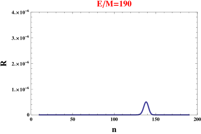
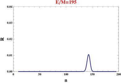
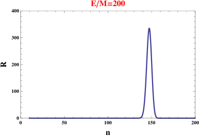
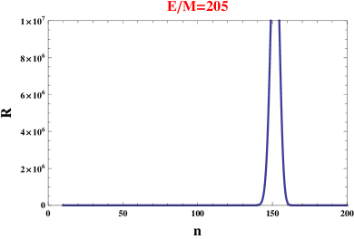
Figure 2: Multi-particle decay rates Eq. (5.2) of a highly-energetic single-particle state into $n$ scalars plotted as function of $n$. The four sub-figures show the energy $E$ fixed at 190$M_{h}$, 195$M_{h}$, 200$M_{h}$ and 205$M_{h}$ and we used $\lambda=1/8$. There is a sharp exponential dependence of the peak rate on the energy. The peak multiplicities $n\sim 150$ in these examples are not far from the maximally allowed values at the edge of the phase space $n_{\rm max}\sim E/M_{h}$.

To illustrate the emergence of Higgsplosion, we plot ${\cal R}_{n}(E)$ of (5.2) in Fig. 2 at fixed values of $E$ and vary $n$. The values of the energy are chosen to zoom on the range where ${\cal R}_{n}(E)$ changes from the exponentially small to exponentially large values. The energy dependence of this transition is very sharp, this fact playing an important role in effectively cutting off at $E_{c}$ the loop integrals contributing to the Higgs mass in the solution to the Hierarchy problem proposed in [3]. It is also easy to understand the peak in the particle number $n$ for each fixed-energy plot in Fig. 2. At relatively low values of $n$ the multi-particle rate is small, as expected, while at the maximal value $n_{\rm max}=E/M_{h}$ the rate is zero again as we have run out of the phase space for the final-state particles; hence the local maximum in $n$ appears before the edge of the phase-space is reached, and is located at the values of $n$ parametrically close to the maximal $n$.

The expression for the multi-particle rate (5.2) should of course not be taken as the full final result for the physical Higgsplosion rate. We have already emphasised that this result is an approximation derived in the simplified scalar model (1.1) and in the simplifying non-relativistic limit. Specifically, our main result (4.27) was derived on the multi-particle threshold, i.e. at $\varepsilon=0$. Hence the higher-order corrections in $\varepsilon$ will be present in the expression for the rate in the $\lambda n$ limit. Denote these corrections $f_{\lambda n;\varepsilon}({\lambda n,\varepsilon})$, so that

$$\Delta_{\rm new}W\,=\,\frac{\lambda n}{\lambda}\,\,f_{\lambda n;\varepsilon}({\lambda n,\varepsilon})\,,$$ (5.4)

and the now modified rate becomes,

$${\cal R}_{n}(E)\,\sim\,\int_{0}^{\varepsilon_{nr}}d\varepsilon\,\left(\frac{\varepsilon}{3\pi}\right)^{\frac{3n}{2}}\exp\left[n\,\left(0.85\,\sqrt{\lambda n}\,+\,\log\lambda n\,+\,f_{\lambda n;\varepsilon}({\lambda n,\varepsilon})\,+\,c\right)\right]$$ (5.5)

where we have included the new correction $n\sim f_{\lambda n;\varepsilon}({\lambda n,\varepsilon})$ and have also made explicit the fact that the $3n/2\log\varepsilon/(3\pi)$ factor in the exponent of the rate (5.2) originated from the integration over the non-relativistic $n$-particle phase-space with a cut-off at $\varepsilon_{nr}<1$. The constant $c$ absorbs various constant factors appearing in the original rate.

The integral above is of course meant to be computed in the large-$n$ limit by finding the saddle-point value $\varepsilon=\varepsilon_{\star}$. The main point of the exercise is to determine (1) whether there is a regime where $\varepsilon_{\star}\ll 1$ so that our near-the-threshold approach is justified, and (2) whether the saddle-point value of the rate itself is large. These requirements should tell us something about the function $f_{\lambda n;\varepsilon}$.

Let us assume that the correction to our result has the form,

$$f_{\lambda n;\varepsilon}({\lambda n,\varepsilon})\,=\,-a\,\varepsilon\,(\lambda n)^{p}\,,$$ (5.6)

where $a$ and $p$ are constants. This function is supposed to represent the higher-order in $\varepsilon$ correction to our result in the small-$\varepsilon$, large-$\lambda n$ limit. The integral we have to compute is,

$${\cal R}_{n}\,\sim\,e^{n\,\left(0.85\,\sqrt{\lambda n}\,+\,\log\lambda n\,+\,\tilde{c}\right)}\,\,\int d\varepsilon\,e^{n\,\left(\frac{3}{2}\log\varepsilon\,-\,a\,\varepsilon\,(\lambda n)^{p}\right)}\,.$$ (5.7)

Denoting the $\varepsilon$-dependent function in the exponent $s(\varepsilon)$,

$$s(\varepsilon)\,=\,\frac{3}{2}\log\varepsilon\,-\,a\,\varepsilon\,(\lambda n)^{p}\,,$$ (5.8)

we can compute the saddle-point,

$$\frac{\partial s(\varepsilon)}{\partial\varepsilon}\,=\,0\quad\Rightarrow\quad\varepsilon_{\star}\,=\,\frac{3}{2}\,\frac{1}{a}\,\frac{1}{(\lambda n)^{p}}\,,$$ (5.9)

and the value of the function $s$ at the saddle-point,

$$s(\varepsilon_{\star})\,=\,-\frac{3}{2}\,\left(p\log\lambda n\,+\,1\,-\,\log\frac{3}{2a}\right)\,.$$ (5.10)

Combining this with the function in the exponent in front of the integral in (5.7) we find the saddle-point value of the rate,

$${\cal R}_{n}(\varepsilon_{\star})\,\sim\,\exp\left[n\,\left(0.85\,\sqrt{\lambda n}\,-\,\left(\frac{3p}{2}-1\right)\log\lambda n\,+\,{\rm const}\right)\right]\,.$$ (5.11)

This is the value of the rate at the local maximum, and since the factor of $\sqrt{\lambda n}$ grows faster than the $-\log\lambda n$ term, the peak value of the rate is exponentially large in the limit of $\sqrt{\lambda n}\infty$. It is also easy to verify that this conclusion is consistent within the validity of the non-relativistic limit. In fact, the value of $\varepsilon$ at the saddle-point is non-relativistic,

$$\varepsilon_{\star}\,=\,\frac{3}{2}\,\frac{1}{a}\,\frac{1}{(\lambda n)^{p}}\,\to\,0\,,\quad{\rm as}\quad\lambda n\to\,\infty\,.$$ (5.12)

We thus conclude that the appearance of the higher-order in $\varepsilon$ corrections to our result in the form (5.6) do not prevent the eventual Higgsplosion in this model at least in the formal limit $\sqrt{\lambda n}\to\infty$ where we have found that

$${\cal R}_{n}(\varepsilon_{\star})\,\gg\,1\,.$$ (5.13)

The growth persists for any constant values of $a$ and $p$. In fact, if $a$ was negative, the growth would only be enhanced. In (5.6) we have assumed that the function goes as $\varepsilon$ to the first power. The higher powers would not change the conclusion, while the effect of $\sim\varepsilon^{0}$ is what is already taken into account in (4.27).

For completeness, we note that only a rather extreme type of corrections would prevent the Higgsplosion in this theory. They would have to be of the form,

$$f_{\lambda n;\varepsilon}({\lambda n,\varepsilon})\,=\,-\,\varepsilon\,e^{(\lambda n)^{p}}\,,$$ (5.14)

which in terms of ${\cal R}_{n}$ would amount to a negative double exponential,

$${\cal R}_{n}\,\sim\,\exp\left[-n\varepsilon\,e^{(\lambda n)^{p}}\right]\,\sim\,\exp\left[-E\,e^{(\lambda n)^{p}}\right]\,,$$ (5.15)

which we find to be rather unlikely.

Our discussion up to now concentrated entirely on a simple scalar field model. If more degrees of freedom were included, for example the $W$ and $Z$ vector bosons and the SM fermions, new coupling parameters (such as the gauge coupling $\alpha_{w}$ and the top Yukawa $y_{t}$) would appear in the expression for the rate along with the final state particle multiplicities. As there are more parameters, the simple scaling properties of ${\cal R}_{n}$ in the pure scalar theory will be modified. If the scaling persists, there will be more to it than the two variables $\lambda n$ and $\varepsilon$. Understanding of how this works and investigating the appropriate weak-coupling / high-multiplicity semiclassical limit or limits is an important task for future work.

One can however consider such effects in the leading order in the loop expansion, i.e. where the $\lambda n$ parameter is considered to be small. Very recently the contributions of virtual top quarks (more generally, fermions and/or scalars coupled to the Higgs) to the multi-Higgs amplitudes on the threshold were computed in [22]. Their result for the case of the top quark is that the threshold amplitude of the pure Higgs theory is multiplied by an overall factor,

$${\cal A}_{n}\,\longrightarrow\,{\cal A}_{n}\,\left(1\,-\,C\,n^{2}\lambda\,\frac{1}{n^{6-4\frac{m_{t}}{M_{h}}}}\,+\,{\cal O}(\lambda^{2})\right)\,,$$ (5.16)

where $m_{t}$ is the top quark mass and the numerical coefficient $C$ for the top-quark correction is

$$C\,=\,C\left(\frac{m_{t}}{M_{h}}\right)\,\simeq\,(8.0+i\,5.8)\frac{\sqrt{3}}{8\pi}\,.$$ (5.17)

What is currently unknown is whether these corrections can exponentiate, and if so, what their effect might be in the appropriate large $\lambda n$ limit. If there is no effective exponentiation of these effects, in our view it would be extremely unlikely to expect that a precise cancellation in the prefactor of the multi-particle rate could occur. If the exponentiation of these effects does occur, as it did for the virtual corrections within the scalar sector itself, the possible effects of it need yet to be understood. We have written the top-quark correction in (5.16) in a suggestive form, singling out the factor of $n^{2}\lambda$. This was done in order to compare its effect to the leading order correction to the ${\cal R}_{n}$ in the scalar theory (cf (4.5)),

$$n^{2}\lambda\,\frac{\sqrt{3}}{4\pi}\,\qquad vs.\qquad n^{2}\lambda\,\frac{1}{n^{6-4\frac{m_{t}}{M_{h}}}}\,2{\rm Re}C\,\simeq\,\frac{n^{2}\lambda}{n^{0.48}}\,\frac{8\sqrt{3}}{4\pi}$$ (5.18)

Formally, there is a parametric suppression of the top-corrections relative to the leading order loop correction in the scalar sector. In the asymptotic limit of large $n$ they would be subleading. The resummation of the loop corrections in the scalar sector is what have resulted in the large $\sqrt{\lambda n}$ effect we have computed. On the other hand, at present little is known about the prospects of resummation or even the sign of the effect related to the top quark corrections. Similarly, important effects should also from including the vector bosons, and these avenues should be pursued in future.

The main conclusion we draw from the results presented in this paper is that we have demonstrated that the Higgsplosion phenomenon is realised above a critical energy/high-multiplicity scale in a concrete QFT settings. The theory we used is the scalar QFT (1.1) with the spontaneous symmetry breaking. The idea of Higgsplosion as a possible solution to the Higgs mass-induced Hierarchy problem also has direct model-building and phenomenological consequences. From the phenomenological perspective the idea is also testable, for example by studying the feasibility of observing of the muti-Higgs and multi-vector-boson production cross-sections at future hadron colliders [16, 21]. The Higgsplosion yield at colliders was recently addressed in Ref. [23]. We believe that studies of Higgsplosion phenomenology offers promising and exciting opportunities for future in particle physics and cosmology.

References

- [1] G. Aad et al. [ATLAS Collaboration], “Observation of a new particle in the search for the Standard Model Higgs boson with the ATLAS detector at the LHC,” Phys. Lett. B 716, 1 (2012) arXiv:1207.7214 [hep-ex].
- [2] S. Chatrchyan et al. [CMS Collaboration], “Observation of a new boson at a mass of 125 GeV with the CMS experiment at the LHC,” Phys. Lett. B 716, 30 (2012) arXiv:1207.7235 [hep-ex].
- [3] V. V. Khoze and M. Spannowsky, “Higgsplosion: Solving the Hierarchy Problem via rapid decays of heavy states into multiple Higgs bosons,” arXiv:1704.03447 [hep-ph].
- [4] D. T. Son, “Semiclassical approach for multiparticle production in scalar theories,” Nucl. Phys. B 477 (1996) 378 hep-ph/9505338.
- [5] A. S. Gorsky and M. B. Voloshin, “Nonperturbative production of multiboson states and quantum bubbles,” Phys. Rev. D 48 (1993) 3843 hep-ph/9305219.
- [6] J. M. Cornwall, “On the High-energy Behavior of Weakly Coupled Gauge Theories,” Phys. Lett. B 243 (1990) 271.
- [7] H. Goldberg, “Breakdown of perturbation theory at tree level in theories with scalars,” Phys. Lett. B 246 (1990) 445.
- [8] M. B. Voloshin, “Multiparticle amplitudes at zero energy and momentum in scalar theory,” Nucl. Phys. B 383 (1992) 233.
- [9] L. S. Brown, “Summing tree graphs at threshold,” Phys. Rev. D 46 (1992) 4125 hep-ph/9209203.
- [10] E. N. Argyres, R. H. P. Kleiss and C. G. Papadopoulos, “Amplitude estimates for multi - Higgs production at high-energies,” Nucl. Phys. B 391 (1993) 42.
- [11] M. B. Voloshin, “Estimate of the onset of nonperturbative particle production at high-energy in a scalar theory,” Phys. Lett. B 293 (1992) 389.
- [12] M. B. Voloshin, “Summing one loop graphs at multiparticle threshold,” Phys. Rev. D 47 (1993) 357 hep-ph/9209240.
- [13] B. H. Smith, “Summing one loop graphs in a theory with broken symmetry,” Phys. Rev. D 47 (1993) 3518 hep-ph/9209287.
- [14] M. V. Libanov, V. A. Rubakov, D. T. Son and S. V. Troitsky, “Exponentiation of multiparticle amplitudes in scalar theories,” Phys. Rev. D 50 (1994) 7553 [hep-ph/9407381].
- [15] M. V. Libanov, V. A. Rubakov and S. V. Troitsky, “Multiparticle processes and semiclassical analysis in bosonic field theories,” Phys. Part. Nucl. 28 (1997) 217.
- [16] V. V. Khoze, “Perturbative growth of high-multiplicity W, Z and Higgs production processes at high energies,” JHEP 1503 (2015) 038 arXiv:1411.2925 [hep-ph].
- [17] J. Jaeckel and V. V. Khoze, “Upper limit on the scale of new physics phenomena from rising cross sections in high multiplicity Higgs and vector boson events,” Phys. Rev. D 91 (2015) no.9, 093007 arXiv:1411.5633 [hep-ph].
- [18] V. V. Khoze, “Diagrammatic computation of multi-Higgs processes at very high energies: Scaling with MadGraph,” Phys. Rev. D 92 (2015) no.1, 014021 arXiv:1504.05023 [hep-ph].
- [19] V. V. Khoze, “Multiparticle Higgs and Vector Boson Amplitudes at Threshold,” JHEP 1407 (2014) 008 arXiv:1404.4876 [hep-ph].
-
[20]
L. D. Landau,
“”On the theory of transfer of energy at collisions I”,
Phys. Zs. Sowiet. 1, 88 (1932);
L. D. Landau and E. M. Lifshitz, “Quantum Mechanics”, Pergamon Press (1977). Chapter VII, Sections 51-52. - [21] C. Degrande, V. V. Khoze and O. Mattelaer, “Multi-Higgs production in gluon fusion at 100 TeV,” Phys. Rev. D 94 (2016) 085031 arXiv:1605.06372 [hep-ph].
- [22] M. B. Voloshin, “Loops with heavy particles in multi Higgs production amplitudes,” arXiv:1704.07320 [hep-ph].
- [23] J. S. Gainer, “Measuring the Higgsplosion Yield: Counting Large Higgs Multiplicities at Colliders,” arXiv:1705.00737 [hep-ph].