Averaging method for systems with separatrix crossing

Abstract

The averaging method provides a powerful tool for studying evolution in near-integrable systems. Existence of separatrices in the phase space of the underlying integrable system is an obstacle for application of standard results that justify using of averaging. We establish estimates that allow to use averaging method when the underlying integrable system is a system with one rotating phase, and the evolution leads to separatrix crossings.

1 Introduction

An averaging method (see, e.g., [5]) is a powerful tool for study a long-term evolution in systems which are small perturbations of integrable systems. Many applications of this method are for one-frequency systems (also called systems with one fast rotating phase). In these cases in the phase space of the corresponding unperturbed system there is a domain foliated by closed trajectories - invariant circles. Averaging of perturbations over these circles provides a closed system for an approximate description of perturbed dynamics in this domain. Typically, in systems under consideration there are several such domains. These domains are bounded by surfaces on which this foliation has singularities. Classical results justifying averaging method [5] guarantee its applicability for description of evolution not too close to these separating surfaces. However, it is rather typical that evolution leads to crossing of these surfaces. The goal of this paper is to provide justification of a modified version of the averaging method for description of such an evolution.

A paradigmatic example of problems considered in this paper is a pendulum under the action of perturbations, e.g., of a small friction, a small constant torque, and a slow change of its length. An unperturbed pendulum could be in one of three regimes of motion: it could rotate in one or other direction, or oscillate. In the phase portrait of the pendulum these three regimes are demarcated by separatrices (Fig. 1). Motion of the pendulum evolves slowly under the action of perturbations. In the process of this evolution the pendulum can change the regime of its motion. In the phase plane the phase point crosses an instant separatrix of the unperturbed pendulum. Evolution of energy far from the separatrix can be described by the averaging method. Classical results justifying this method [5] are not applicable in the case of crossings of a separatrix. Moreover, this crossing leads to a remarkable probabilistic scattering. Initial data for different outcomes of separatrix crossings are mixed, and it is reasonable to consider each outcome as a random event with a definite probability. This probabilistic approach was first described in a similar problem in [21] and then independently in [14].

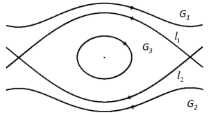
Figure 1: Phase portrait of a pendulum.

A natural way to describe evolution in the considered system is to use averaging method up to arrival to the separatrix, to calculate probabilities of capture into different domains at the separatrix, and to use the averaging method starting from the separatrix in the domain in which the system continues its evolution. In the current paper we justify such an approach for a rather wide class of one-frequency systems that change a qualitative character of their motion in the process of evolution. The obtained estimates of the accuracy of the averaging method are sharp.

Part of results of this paper was announced (without proofs) in [26] (see also [4], Subsection 6.1.10) on the basis of estimates in [25].

2 Averaging method and averaging theorem for the separatrix crossing

In this section an averaging theorem is formulated that justifies the averaging method for description of the separatrix crossing. The proof is based on propositions given in Sections 3, 4, 5. There are probability phenomena due to separatrix crossing. Hence the recipe of the averaging method here includes calculations of the corresponding probabilities, and the averaging theorem justifies these calculations. All considerations are for systems of the form (2.1) below. We explain in the Appendix relation of this form to the general form of one-frequency systems with separatrix crossings.

2.1 Outline of the problem

We consider systems described by differential equations of the form

$$\dot{q} = \frac{\partial E}{\partial p}+\varepsilon f_{1},\,\dot{p}=-\frac{\partial E}{\partial q}+\varepsilon f_{2},\,\dot{z}=\varepsilon f_{3}\,,$$ (2.1)

$$E = E(p,q,z),\,f_{i}=f_{i}(p,q,z,\varepsilon),i=1,2,3,\,(p,q)\in\mathbb{R}^{2},z\in\mathbb{R}^{l-2}\,.\$$

Here $\varepsilon>0$ is a small parameter characterising the rate of evolution. For $\varepsilon=0,\,z={\rm const}$ we have an unperturbed system for $p,q$, which is a Hamiltonian system with one degree of freedom. The function $E$ is an unperturbed Hamiltonian, and the functions $\varepsilon f_{i}$ are the perturbations. It is supposed, that there are separatrices in the phase portrait of the unperturbed system Fig. 2. In the course of evolution the projection of the phase point onto the plane $(p,q)$ crosses a separatrix.

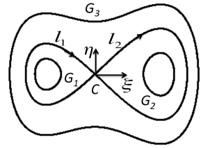
Figure 2: Phase portrait of the unperturbed system.

Far from the separatrices instead of $(p,q)$ it is possible to use the variables $h=E$ and $\varphi$, where $\varphi$ is “the angle” (from the pair “action-angle” variables [2] of the unperturbed system). Then for $h,z,\varphi$ we get the perturbed system having the standard form of system with one rotating phase [5]: in this system $h,z$ are called slow variables, $\varphi$ is the rotating phase. It is a classical result that the averaged with respect to $\varphi$ system describes the evolution of $h,z$ far from separatrices with accuracy $O(\varepsilon)$ during the time interval of order $1/\varepsilon$. At the separatrices the frequency of the unperturbed motion vanishes, and also the equations in variables $h$,$z$,$\varphi$ have singularities. In a region that includes a separatrix, the conditions of the classical theorem about accuracy of the averaging [5] fail and the applicability of the averaging method for the description of the evolution near the separatrices requires a justification.

Separatrix crossing leads to probability phenomena [21, 14, 1, 15]. As a simple example let as consider the motion of a particle in one dimension in double-well potential, Fig. 3a, perturbed by a small, of order $\varepsilon$, dissipation [1]. Phase portrait of the perturbed system is shown in Fig. 3b, where the initial conditions for the capture into the region, surrounded by the right separatrix loop, are shaded.

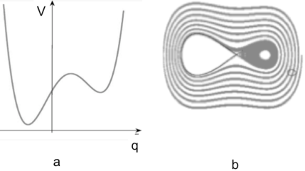
Figure 3: a) Double-well potential. b) Effect of a small friction.

The shaded strips far from the saddle have width of order $\varepsilon$ and form a spiral with a step of order $\varepsilon$. Therefore small, of order $\varepsilon$, change of the initial conditions can change the result of evolution. As the initial conditions are always known only with some finite accuracy, the deterministic approach to the problem fails when $\varepsilon\to 0$. But it is possible to define in some natural way and to calculate the probabilities of capture into different regions after the separatrix crossing [1].

For systems of such types, a procedure of an approximate description of the evolution consists of using the averaged system up to the separatrix and calculation of the probability of capture into one or another region on the separatrix. It will be seen, that for majority of initial conditions this procedure describes the behaviour of the slow variables with accuracy $O(\varepsilon\ln\varepsilon)$ during time of order $1/\varepsilon$. The measure of the “bad” set of initial conditions, for which this description is not valid, tends to $0$ faster, than any given power of $\varepsilon$ as $\varepsilon\to 0$. The general formula for the probability of the capture into one or another region (in the sense of definition in [1]) also will be proved.

2.2 Formulation of Hypotheses

System (2.1) is considered for $(p,q,z)\in D,\mid\varepsilon\mid<\varepsilon_{1}$, where $D$ is a bounded domain in $\mathbb{R}^{l},\ \varepsilon_{1}={\rm const}$. We denote $B$ the projection of $D$ onto $z$-space, and $G=G(z)$ the section of $D$ by the two-dimensional plane $z={\rm const}$. It is supposed that each domain $G(z)\subset\mathbb{R}^{2}$ is composed of the whole trajectories of the unperturbed system. It is supposed that the following assumptions are satisfied.

$\bf{A}$. The function $E$ is of smoothness $C^{3}$, and the functions $f_{i}$ are of smoothness $C^{2}$ with respect to $p,q,z$. Functions $f_{i}$ have one continuous derivative with respect to $\varepsilon$.

$\bf{B}$. For $z\in B$ the phase portrait of the unperturbed system in the domain $G(z)$ has the form shown in Fig. 2. The unstable stationary point $C$ is a non-degenerate saddle point. The separatrices $l_{1}=l_{1}(z)$ and $l_{2}=l_{2}(z)$ divide the unperturbed phase portrait into three regions $G_{\nu}=G_{\nu}(z),\,\nu=1,2,3$. In what follows we assume that the Hamiltonian $E$ is normalised in such a way, that $E=0$ at the saddle point $C$, and therefore, on the separatrices. Then $E>0$ in the region $G_{3}$, $E<0$ in the regions $G_{1}$ and $G_{2}$. We denote $l_{3}=l_{1}\cup l_{2}$.

$\bf{C}$. Introduce quantities

$$\Theta_{\nu}(z) = -\oint_{l_{\nu}}\left(\frac{\partial E}{\partial q}f_{1}^{0}+\frac{\partial E}{\partial p}f_{2}^{0}+\frac{\partial E}{\partial z}f_{3}^{0}\right)dt\,,\ \nu=1,2,$$ (2.2)

$$\Theta_{3}(z) = \Theta_{1}(z)+\Theta_{2}(z)\,.$$

Integrals in (2.2) are calculated along the unperturbed separatrices parametrized by the time $t$ of the unperturbed motion; $f_{i}^{0}=f_{i}(p,q,z,0),\,i=1,2,3$. Integrals (2.2) are improper, because the motion along a separatrix takes infinite time. Our normalisation of $E$ guarantees the convergence of the integrals as it is proved at the end of this section. We assume that the values $\Theta_{\nu},\,\nu=1,2,3$ are different from zero. In what follows, for certainty, the values $\Theta_{\nu},\,\nu=1,2,3$ are supposed to be positive.

Let us explain the meaning of the condition $\bf{C}$. In the region $G_{\nu}$ for small $|E|>\varepsilon$, in the perturbed motion, a phase point makes rounds that are close to the unperturbed separatrix $l_{\nu}$. The change of the value of $E$ during one such round is close to the value $-\varepsilon\Theta_{\nu}$ . Therefore, for phase points with small $|E|$, condition $\bf C$ ensures an approach the separatrix in the region $G_{3}$ and a departure from the separatrix in the regions $G_{1}$ and $G_{2}$. The convergence of integrals (2.2) is a corollary of the following assertion.

Lemma 2.1

The first derivatives of the function $E$ with respect to $p,q,z$ vanish at the point $C$.

Proof. The derivatives with respect to $p,q$ vanish at the point $C$ because the point $C$ is an equilibrium position of the unperturbed system. Let $p_{C}(z),q_{C}(z)$ be coordinates of the point $C$. The Hamiltonian is normalised by the condition $E(p_{C}(z),q_{C}(z),z)\equiv 0$. Calculating the derivative of this equality with respect to $z$ and taking into account that $\frac{\partial E}{\partial p}=\frac{\partial E}{\partial q}=0$ at the point $C$, we get that $\frac{\partial E}{\partial z}=0$ at the point $C.\hskip 199.16928pt\square$

Lemma 2.1 implies that

$$(\partial E/\partial\alpha)/\sqrt{(\partial E/\partial p)^{2}+(\partial E/\partial q)^{2}},\alpha=p,q,z,$$

tend to finite limits as a point $(p,q)$ tends to the point $C$ along a separatrix. Let us use in the integrals (2.2) the arc length along the separatrix as a new independent variable. Then integrands do not have singularities, and therefore integrals (2.2) converge. Moreover, $\Theta_{\nu}$ are smooth functions of $z$.

2.3 Averaged system

Let us define the averaged system separately for each region $G_{\nu}$ first. Let

$$\varSigma_{\nu}=\{(h,z)\colon z\in B,h=E(p,q,z),(p,q)\in G_{\nu}(z)\},\ \nu=1,2,3\,.$$

The averaged in the region $G_{\nu}$ system is, by definition, the following system of differential equations in $\Sigma_{\nu}$:

$$\dot{h} = {\varepsilon\over T}\oint_{E=h}(\frac{\partial E}{\partial q}f_{1}^{0}+\frac{\partial E}{\partial p}f_{2}^{0}+\frac{\partial E}{\partial z}f_{3}^{0})dt\,,$$ (2.3)

$$\dot{z} = {\varepsilon\over T}\oint_{E=h}f_{3}^{0}dt\,.$$

Here integrals are calculated along the level line $E=h$ of the Hamiltonian situated in the domain $G_{\nu}(z)$. This level line is parametrized by the time $t$ of the unperturbed motion along it, and $T=T(h,z)$ is the period of this motion. To write down this averaged system we calculate the rate of changing of $h=E(p,q,z)$ and $z$ in the perturbed system, and then average the obtained expressions over $t$ along the level line $E=h$ (for $\varepsilon=0$ in the arguments of $f_{i}$). This averaging is equivalent to the averaging over the angular variable $\varphi$ discussed in Subsection 2.1.

The period $T$ grows proportionally to $-\ln|h|$ in the principal approximation as $h\to 0$ (see Lemma 3.3). When $h=0$ it is reasonable to extent the definition of the right hand sides of (2.3) by continuity, putting

$$\dot{h}\mid_{h=0}\,=0,\ \dot{z}\mid_{h=0}\,=\varepsilon f_{3C}^{0}\,,$$

where $f_{3C}^{0}$ is the value of the function $f_{3}^{0}$ at the point $C$. Now we can combine three averaged systems in different regions into one “whole” averaged system. The phase space of the “whole” averaged system is a singular manifold, glued of three parts $\Sigma_{1},\Sigma_{2}$ and $\Sigma_{3}$ along the set $\{h=0\}$, Fig. 4. We will call the set $\{h=0\}$ the separatrix for the averaged system.

Figure 4: The phase space of the averaged system.

According to condition $\bf{C}$,  $\dot{h}<0$ in the averaged system for small $h\neq 0$ in all regions.

Definition. A solution $H(\tau),\;Z(\tau),\;\tau=\varepsilon t$, of the averaged system in $G_{\nu}$ such that $H(\tau)\to 0$, $Z(\tau)\to z_{*}$ as $\tau\to\tau{}_{*}-0$ (for the region $G_{3}$) or $\tau\to\tau{}_{*}+0$ ( for the regions $G_{1,2}$) is called a solution crossing the separatrix at the point $z_{*}$ at the moment $\tau{}_{*}$.

The following lemma is proved in Subsection 3.6.

Lemma 2.2

a) For any $z_{*}\in B$, $\tau{}_{*}$, and $\nu=1,2,3$ there exists a unique solution of the averaged system in $G_{\nu}$ crossing the separatrix at the point $z_{*}$ at the moment $\tau{}_{*}$.

b). If $z_{0}\in B$, then for small enough $|h_{0}|$ the solution $H(\tau),\;Z(\tau)$ of the averaged system with the initial conditions $H(\tau{}_{0})=h_{0},Z(\tau{}_{0})=z_{0}$ crosses the separatrix at some moment $\tau=\tau{}_{*}$ ($\tau{}_{*}>\tau_{0}$, if $h_{0}>0$ and $\tau{}_{*}<\tau{}_{0}$ if $h_{0}<0$).

Take any point $(p_{0},q_{0},z_{0})\in D$ such that $(p_{0},q_{0})\in G_{3}(z_{0})$. Denote $h_{0}=E(p_{0},q_{0},z_{0})$. Consider the solution $(H_{3}(\tau),\;Z_{3}(\tau))$ of the averaged system in $G_{3}$ with the initial condition $(h_{0},z_{0})$ at $\tau=0$ (Fig. 4). Suppose that this solution crosses the separatrix at some $\tau=\tau{}_{*}$, i.e. $H_{3}(\tau{}_{*})=0,\;Z_{3}(\tau{}_{*})=z_{*}$. According to Lemma 2.2, we can consider the solution $(H_{\nu}(\tau),Z_{\nu}(\tau))$ of the system averaged in $G_{\nu}$, $\nu=1,2$ with the initial condition $(0,z_{*})$ at $\tau=\tau{}_{*}$. This solution is well defined for $\tau$ close enough to $\tau{}_{*}$, $\tau>\tau{}_{*}$. For an approximate description of the behaviour of the values $E,\;z$ in the perturbed system (2.1) we use the solution $(H_{3},\;Z_{3})$ for $0\leq\varepsilon t\leq\tau{}_{*}$, and the solution $(H_{\nu},Z_{\nu})$ for $\varepsilon t>\tau{}_{*}$ with $\nu=1$ or $2$, if the phase point has been captured into the region $G_{\nu}$ after the separatrix crossing. We define for $\tau\leq\tau{}_{*}$ the functions $H_{\nu},\;Z_{\nu},\ \nu=1,2$, by the relations $H_{\nu}(\tau)=H_{3}(\tau),\;Z_{\nu}(\tau)=Z_{3}(\tau)$. These functions $(H_{\nu},Z_{\nu})$ are called the solutions of the averaged system with the initial condition $(h_{0},z_{0})$ at $t=0$.

We attribute the probability $\Theta_{\nu}(z_{*})/\Theta{}_{3}(z_{*})$ to the capture into $G_{\nu}$ of the initial point $(p_{0},q_{0},z_{0})$. The meaning of this definition of the probability will be clear from the results of Subsection 2.4. The function $P_{\nu}$ defined by the formula

$$P_{\nu}(z)=\Theta_{\nu}(z)/\Theta_{3}(z)$$ (2.4)

will be called the probability of the capture into $G_{\nu},\,\nu=1,2$, at the separatrix.

We will need a lemma which allows to estimate a distance between two solutions of the averaged system with initial conditions near the separatrix.

Lemma 2.3

Let two solutions of the averaged system, $(H_{\nu}(\tau),Z_{\nu}(\tau))$ and $({{H}^{\prime}_{\nu}(\tau)},{{Z}^{\prime}_{\nu}(\tau))},\ 0\leq\tau\leq K$, be given. Suppose that for some $\tau_{0}\in[0,K]$ and some $\delta>0$ these solutions satisfy the following condition:

$$|H_{\nu}(\tau_{0})|+|{H}^{\prime}_{\nu}(\tau_{0})|+|Z_{\nu}(\tau_{0})-{Z}^{\prime}_{\nu}(\tau_{0})|<\delta.$$

If $\delta$ is small enough, then for $0\leq\tau\leq K$ the following estimate is valid:

$$|H_{\nu}(\tau)-{H}^{\prime}_{\nu}(\tau)|+|Z_{\nu}(\tau)-{Z}^{\prime}_{\nu}(\tau)|<O\left(\delta+{\delta|\ln\delta|\over 1+|\ln|H_{\nu}(\tau)||}\right)\,.$$

The proof is given in Subsection 3.6.

In what follows, the action $I$ of the unperturbed system will be important. The action $I=I(h,z)$ of the unperturbed trajectory $E=h$ in the region $G_{\nu}$ is the area enclosed by this trajectory, divided by $2\pi$. We have [19]

$$\frac{\partial I}{\partial h}=\frac{1}{2\pi}T\left(h,z\right),$$ (2.5)

$$\frac{\partial I}{\partial z}=-\frac{1}{2\pi}\oint_{E=h}\frac{\partial E}{\partial z}dt\,.$$ (2.6)

With the aid of the formulas (2.5) and (2.6) the rate of change of $I$ along a trajectory of the averaged system is found to be:

$$2\pi{dI\over dt} = \varepsilon\oint_{E=h}({\partial E\over\partial q}f_{1}^{0}+{\partial E\over\partial p}f_{2}^{0}+{\partial E\over\partial z}f_{3}^{0})dt$$ (2.7)

$$- {\varepsilon\over T}\oint_{E=h}{\partial E\over\partial z}dt\ \oint_{E=h}f_{3}^{0}dt\,.$$

A corollary of the formula (2.6) when $h\to 0$ is the following useful formula for the areas $S_{1,2}=S_{1,2}(z)$ of the regions $G_{1,2}$ and the area $S_{3}=S_{3}(z)$ of the region $G_{1}\cup G_{2}$:

$${\partial S_{\nu}\over\partial z}=-\oint_{l_{\nu}}{\partial E\over\partial z}dt,\nu=1,2,3\,.$$ (2.8)

From (2.2) for the averaged system in the region $G_{\nu}$ we get:

$$\lim_{h\to 0}{d\over dt}(2\pi I-S_{\nu})=-\varepsilon\Theta{}_{\nu}(z),\ \nu=1,2,3\,.$$ (2.9)

A consequence of this equation is the above-mentioned property (see Lemma  2.2) that for solutions of the averaged system with small $|h|$ the arrival at the separatrix takes a finite time (in the region $G_{3}$ this time is positive, in the regions $G_{1,2}$ it is negative).

2.4 Estimates in the averaging method

Let a point $\hat{M}_{0}=(\hat{p}_{0},\hat{q}_{0},\hat{z}_{0})$ belong to the region $D$, and let $\hat{I}_{0},\hat{\varphi}_{0}$ be the values of the action-angle variables $I,\varphi$ at this point. The following sets are well defined and lie in $D$ for small enough $\delta$:

$$U^{\delta} = \{p,q,z\ :\ |z-\hat{z}_{0}|<\delta,|I-\hat{I}_{0}|<\delta,|\varphi-\hat{\varphi}_{0}|<\delta\}\,,$$ (2.10)

$$W^{\delta} = \{p,q,z\ :\ |z-\hat{z}_{0}|<\delta,|I-\hat{I}_{0}|<\delta\}\,.$$

Denote $\hat{h}_{0}=E\left(\hat{p}_{0},\hat{q}_{0},\hat{z}_{0}\right)$. We assume that solutions of the averaged system with initial data $(\hat{h}_{0},\hat{z}_{0})$ are well defined for $0\leq\tau\leq K$ and cross the separatrix at some $\tau=\hat{\tau}_{*}$, $z=\hat{z}_{*}$. Denote:

• $(p(t),q(t),z(t))$ the solution of the perturbed system (2.1) with initial data $(p_{0},q_{0},z_{0})\in U^{\delta}$ at $t=0$,

• $h(t)=E(p(t),q(t),z(t))$ the value of the Hamiltonian along this solution,

• $h_{0}=h\left(0\right)$,

• $(H_{\nu},Z_{\nu}),\ \nu=1,2$, the solutions of the averaged system with the initial condition $(h_{0},z_{0})$ at $\tau=0$,

• $\tau_{*}$ the moment of separatrix crossing for the solutions $(H_{\nu},Z_{\nu})$.

The value $\delta$ is supposed to be small enough so that the solutions $(H_{\nu},Z_{\nu}),\ \nu=1,2$, are well defined for $0\leq\tau\leq K$, and $\tau_{*}<K$. Fix any natural number $r\geq 2$. In what follows $K_{i}$ (and afterwards $k_{i},c_{i},d_{i},\nu_{i}$) are positive constants, i.e. values independent of $\varepsilon,\delta$ and initial conditions $(p_{0},q_{0},z_{0})\in W^{\delta}$. The appearance of $K_{i}$ in some relation is equivalent to the assertion that there exists $K_{i}$ satisfying this relation for small enough $\varepsilon>0,\delta>0,\varepsilon<\delta^{2}$ (and similarly for other constants). The following theorem summarises the principal features of the averaging method for separatrix-crossing orbits:

Theorem 1

There exists a representation $U^{\delta}=U_{1}^{\delta}\cup U_{2}^{\delta}\cup v$ with the following properties.

I. If $(p_{0},q_{0},z_{0})\in U_{\nu}^{\delta},\ \nu=1,2$, then the behaviour of $E,z$ in the perturbed system is described approximately by the solution $(H_{\nu},Z_{\nu})$ of the averaged system, and the following estimates hold

$$|h(t)-H_{\nu}(\varepsilon t)|+|z(t)-Z_{\nu}(\varepsilon t)| < K_{1}\varepsilon\quad\mbox{for}\quad 0\leq\varepsilon t\leq\tau_{*},$$ (2.11)

$$|h(t)-H_{\nu}(\varepsilon t)|+|z(t)-Z_{\nu}(\varepsilon t)| < K_{1}\varepsilon+{K_{2}\varepsilon|\ln\varepsilon|\over 1+|\ln|H_{\nu}(\varepsilon t)||}\quad\mbox{for}\quad\tau_{*}\leq\varepsilon t\leq K\,.$$

For $0\leq\varepsilon t\leq\tau_{*}-K_{3}\varepsilon|\ln\varepsilon|$ the point $(p(t),q(t))$ moves in the region $G_{3}(z(t))$, while for $\tau_{*}+K_{3}\varepsilon|\ln\varepsilon|\leq\varepsilon t\leq K$ it moves in the region $G_{\nu}(z(t))$.

II.

$$\left|{\hbox{\em mes}\,U_{\nu}^{\delta}\over\mbox{\em mes}\,U^{\delta}}-{\Theta_{\nu}(\hat{z}_{*})\over\Theta_{3}(\hat{z}_{*})}\right|<K_{4}\left(\delta+{\varepsilon|\ln\varepsilon|\over\delta}\right).$$

III. $\hbox{\em mes}\,v<k_{5}\varepsilon^{r}\delta^{-1}\hbox{\em mes}\,U^{\delta}$.

Here $\hbox{\em mes}\,(\cdot)$ is the standard phase volume in $\mathbb{R}^{l}$ .

This theorem will be proved by means of a series of propositions established in the following three Sections (Propositions 2.1, 2.2, 2.3).

It is natural to consider the relative measure of the set of points from a small neighbourhood of $\hat{M}_{0}$ that will be captured into the region $G_{\nu},\nu=1,2$ for small $\varepsilon$ as the value at the point $\hat{M}_{0}$ of the probability density of capture into $G_{\nu}$. This approach is formalised as follows (cf. [1]).

Definition The value at the point $\hat{M}_{0}$ of the probability density of capture into $G_{\nu}\,,\nu=1,2\,,$ (or, for brevity, the probability of capture of $\hat{M}_{0}$ into $G_{\nu}$) is

$$Q_{\nu}(\hat{M}_{0})=\lim_{\delta\to 0}\lim_{\varepsilon\to 0}{\hbox{mes}\,U_{\nu}^{\delta}\over\hbox{mes}\,U^{\delta}}\,.$$ (2.12)

Corollary 2.1

The probability of capture of the point $\hat{M}_{0}$ into the region $G_{\nu}$ is given by the formula

$$Q_{\nu}(\hat{M}_{0})={\Theta_{\nu}(\hat{z}_{*})\over\Theta_{3}(\hat{z}_{*})},\ \nu=1,2\,.$$ (2.13)

By means of the function $P_{\nu}$ defined by equation (2.4) – the probability of the capture into $G_{\nu}$ at the separatrix – the last formula can be rewritten in the form

$$Q_{\nu}(\hat{M}_{0})=P_{\nu}(\hat{z}_{*}),\ \nu=1,2\,.$$

Remarks

1. The formulation of the problem of separatrix-crossing has been described in the context of an eight-figure separatrix that is being approached by orbits of the perturbed and averaged systems. It will be clear from the nature of the estimates in the succeeding sections, that the basic results embodied in Theorem 1 can be carried over to the other geometric pictures of separatrix-crossing that are possible in $\mathbb{R}^{2}$. In fact, the phase space need not be $\mathbb{R}^{2}$. It could, for example, be a cylinder or a sphere. The important hypotheses are those demanding the non-degeneracy of the saddle equilibrium and the non-vanishing of the numbers $\Theta_{\nu},\;\nu=1,2,3$ (see Appendix). These conditions may be relaxed: they are needed only when the orbit approaches the separatrix. During the evolution prior to that time, these conditions are not needed. Metamorphoses of the phase portrait may take place as long as the phase point is far from separatrices when this happens. Situations wherein the crossing of a separatrix occurs for values of $z$ for which $\Theta_{\nu}=0$ or at which the non-degeneracy condition for the saddle fails are viewed as degenerate, and the estimates of the averaging method will in general be poorer in these cases. Examples of separatrix-crossing near a “newborn” saddle are considered in [20, 18, 16, 11].

2. The conclusion that the error in the use of the averaging method is $O(\varepsilon\ln\varepsilon)$, which follows from Theorem 1, cannot be improved. This follows from asymptotic formulas for change of the adiabatic invariant at a separatrix in Hamiltonian systems ([27], [9], [23], [24]) and also for systems perturbed by a weak dissipation [7].

3. The assertion of the Theorem 1 remains valid if the standard volume $\hbox{mes}\,(\cdot)$ is replaced by any measure in $\mathbb{R}^{l}$ that has a smooth density, independent of $\varepsilon$, with respect to the standard volume. The formula for the probability given by (2.12) and (2.13) remains valid if $U^{\delta}$ is any domain with piecewise-smooth boundary having diameter $\delta$ (but in this case the estimate in the right hand side in part II of the Theorem  1 may not be satisfied).

4. For the example of motion of a particle in one dimension in double-well potential perturbed by a small dissipation the formula for probability is given in [1]. The proof is contained in [8].

5. A different approach for introducing probability was suggested in [28, 13]. White noise of order $\varepsilon\delta$ was added to the right-hand side of equations (2.1), in the case when the parameter $z$ is absent from the problem. In this problem, capture into one or another region becomes a genuinely random event. Again taking the limit of the probability of capture as $\varepsilon\to 0$ (first) and $\delta\to 0$, one recovers the same formula for the probability as that found in Subsection 2.4 above.

6. D.V.Anosov has suggested yet another approach for introducing probability in the considered problem. Denote $\varkappa_{\nu}(\varepsilon_{0})$ the measure of the set of values $\varepsilon\in(0,\varepsilon_{0}]$ such that $\hat{M}_{0}\in U_{\nu}^{\delta}$ for these values of $\varepsilon$, $\nu=1,2$. Then we define the probability of capture of $\hat{M}_{0}$ into $G_{\nu}$ as $\lim_{\varepsilon_{0}\to 0}\varkappa_{\nu}(\varepsilon_{0})/\varepsilon_{0}$. This definition was not discussed in a literature. One can show that, e.g. for the case when $f_{1}=f_{2}=0$, $f_{3}={\rm const}$ in equations (2.1) this probability is again given by formula (2.13). It looks plausible that this is the case for the general form of system (2.1) as well.

7. An important open question is when results of consecutive crossings of separatrices can be considered as statistically independent. This is not the case, for example, if (2.1) is a Hamiltonian system with slowly varying parameter, and $\Theta_{1}\equiv\Theta_{2}$ [10]. However, it looks as a reasonable hypothesis that typically there is such an independence.

2.5 Derivation of the estimates in the averaging method

In this subsection Theorem 1 is derived from several principal Propositions describing approach the separatrix, passage through its narrow neighbourhood, and departure from the separatrix. These Propositions are proved in Sections 3, 4, 5. Approach the separatrix is described by the following assertion.

Proposition 2.1

For all initial conditions $(p_{0},q_{0},z_{0})\in W^{\delta}$ and for $t>0$ while $H_{3}(\varepsilon t)\geq k_{1}\varepsilon$ the following estimates are valid:

$$|h(t)-H_{3}(\varepsilon t)|+|z(t)-Z_{3}(\varepsilon t)|=O(\varepsilon),\ \frac{1}{2}H_{3}(\varepsilon t)\leq h(t)\leq 2H_{3}(\varepsilon t)\,.$$

Departure from the separatrix in the regions $G_{1,2}$   is described by an analogous assertion.

Proposition 2.2

Let a moment of time $t^{\prime}\in[0,K/\varepsilon]$ exist such that $h(t^{\prime})=-k_{2}\varepsilon,(p(t^{\prime}),q(t^{\prime}))\in G_{\nu}(z(t^{\prime})),\ \nu=1,2,\ |\varepsilon t^{\prime}-\tau_{*}|+|Z(t^{\prime})-Z_{3}(\tau_{*})|<k_{3}^{-1}$. Then for $t^{\prime}\leq t\leq K/\varepsilon$ the behaviour of $E,z$ is approximately described by the solution $(H^{\prime}_{\nu},Z^{\prime}_{\nu})$ of the averaged in $G_{\nu}$ system with the initial condition $h(t^{\prime}),z(t^{\prime})$ at $\tau=\varepsilon t^{\prime}$ as follows:

$$|h(t)-H^{\prime}_{\nu}(\varepsilon t)|+|z(t)-Z^{\prime}_{\nu}(\varepsilon t)|=O\left(\frac{\varepsilon\ln\varepsilon}{1+|\ln|H^{\prime}_{\nu}(\varepsilon t)||}\right)\!,\,2H^{\prime}_{\nu}(\varepsilon t)\leq h(t)\leq\frac{1}{2}H^{\prime}_{\nu}(\varepsilon t)$$

It follows from Proposition 2.1 that there exists a moment of time $t_{-}=t_{-}(p_{0},q_{0},z_{0},\varepsilon)$ such that at this moment $h(t)=2k_{1}\varepsilon$ for the first time. Let $t_{+}=t_{+}(p_{0},q_{0},z_{0},\varepsilon)$ be the moment of time such that at this moment $h(t)=-k_{2}\varepsilon$ for the first time at the segment $[0,K/\varepsilon]$. The moment of time $t_{+}$ is defined, in general, not for all initial conditions. The following assertion describes passage through a narrow neighbourhood of the separatrices during the interval of time $t_{-}\leq t\leq\ t_{+}$.

Proposition 2.3

There exists a representation $W^{\delta}=W^{\delta}_{3}\cup w$ such that ${\rm mes}\,w=O(\varepsilon^{r})\,{\rm mes}\,W^{\delta}$ and for $(p_{0},q_{0},z_{0})\in W_{3}^{\delta}$ the moment of time $t_{+}$ is well defined and $t_{+}=t_{-}+O(\ln\varepsilon)$. For $t_{-}\leq t\leq\ t_{+}$ and for $\nu=1,2$ the following estimate holds:

$$|h(t)|+|H_{\nu}(\varepsilon t)|+|z(t)-Z_{\nu}(\varepsilon t)|=O(\varepsilon)\,.$$

Let $W_{\nu}^{\delta},\,\nu=1,2$, be the sets of points $(p_{0},q_{0},z_{0})\in W_{3}^{\delta}$ such that $(p(t_{+}),q(t_{+}))\in G_{\nu}(z(t_{+}))$.

Proposition 2.4

The measure of the set $W_{\nu}^{\delta}$ is estimated as

$${\rm mes}\,W_{\nu}^{\delta}=\int_{W^{\delta}}P_{\nu}(Z_{3}(\tau_{*}))dp_{0}dq_{0}dz_{0}+O(\varepsilon\ln\varepsilon\,\delta^{-1}\,{\rm mes}\,W^{\delta}),\ \nu=1,2\,.$$

Here $(H_{3}(\tau),Z_{3}(\tau))$ is the solution of the averaged system with the initial condition $H_{3}(0)=E(p_{0},q_{0},z_{0}),Z_{3}(0)=z_{0}$, and $\tau_{*}$ is the moment of separatrix crossing for this solution, $dz_{0}$ is the standart volume element in $\mathbb{R}^{l-2}$.

Denote $U_{\nu}^{\delta}=U^{\delta}\cap W_{\nu}^{\delta},\ v=U^{\delta}\cap w$.

Proposition 2.5

The measure of the set $U_{\nu}^{\delta}$ meets the estimate of part $I\!I$ in Theorem 1.

For $0\leq t\leq t_{+}$ the estimates in Theorem 1 hold due to the estimates of Propositions 2.2 and 2.3. From these estimates we get also that it is possible to choose $t_{+}$ as $t^{\prime}$ in Propositions 2.2. Then at $t=t_{+}$ the distance between solutions $(H^{\prime}_{\nu},Z^{\prime}_{\nu})$ and $(H_{\nu},Z_{\nu})$ is $O(\varepsilon)$. Therefore from Lemma 2.3 and Proposition 2.2 we get the estimates in Theorem 1 for $t_{+}\leq t\leq K/\varepsilon$. This completes the proof of Theorem 1.

To proof Corollary 2.1 it is enough to consider a cover of $U^{\delta}$ by the union of sets

$$U_{j_{1},j_{2},j_{3}}^{\kappa} = \{p,q,z\colon|z-\hat{z}_{j_{1}}|\leq\kappa,|I-\hat{I}_{j_{2}}|\leq\kappa,|\varphi-\hat{\varphi}_{j_{3}}|\leq\kappa\},$$ (2.14)

$${\hat{z}_{j_{1}}} = \hat{z}_{0}+2\kappa j_{1},\ \hat{I}_{j_{2}}=\hat{I}_{0}+2\kappa j_{2},\ \hat{\varphi}_{j_{3}}=\hat{\varphi}_{0}+2\kappa j_{3}\,.$$

Here $j_{2},j_{3}$ are integer numbers, and $j_{1}$ is an integer $(l-2)$-dimensional vector. Then one should apply Theorem 1 to those of sets $U_{j_{1},j_{2},j_{3}}^{\kappa}$, which intersect $U^{\delta}$. Now proceed to the limit first as $\varepsilon\to 0$ and then as $\kappa\to 0$. We get the formula

$$\lim_{\varepsilon\to 0}\hbox{mes}\,U_{\nu}^{\delta}=\int_{U^{\delta}}P_{\nu}(Z_{3}(\tau_{*}))dp_{0}dq_{0}dz_{0}$$

which implies Corollary 2.1.

3 Estimates of the accuracy of the averaging method up to separatrix

In this section the proof of Proposition 2.1 is given. The proof of Proposition 2.2 is entirely analogous, and only a sketch of it is given. We use several lemmas, which are formulated in Subsections 3.1, 3.2. This lemmas are proven in Subsections 3.4, 3.5.

Only motion in the region $G_{3}$ is considered in the principal part of this section. Thus we will omit index $\nu=3$ at solution $(H_{\nu},Z_{\nu})$. The following notation is used: $I(h,z)$ - the value of the “action” variable for the trajectory $E=h$ of the unperturbed system, $j(t)=I(h(t),z(t)),J(\varepsilon t)=I(H(\varepsilon t),Z(\varepsilon t))$.

Below $z\in B-c_{1}^{-1},\,(p,q,z)\in D-c_{1}^{-1}$ in all estimates, and the constant $c_{1}$ is chosen in such a way that $3c_{1}^{-1}$-neighbourhood of the set $\{z\colon z=Z_{\nu}(\tau),\nu=1,2;\tau\in[0,K]\}$ belongs to $B$, and $3c_{1}^{-1}$-neighbourhood of the set

$$\{(p,q,z)\colon z=Z_{\nu}(\tau),E(p,q,z)=H_{\nu}(\tau),\ \nu=1,2;\,\tau\in[0,K]\}$$

belongs to $D$.

3.1 Lemmas on unperturbed motion

Let $\varphi=\varphi(p,q,z,\varepsilon)$ and $\psi=\psi(p,q,z,\varepsilon)$ be smooth functions, and $\varphi$ vanish at the saddle point $C$ identically with respect to $z,\varepsilon$. Let $0<h<1/2,z\in B-c_{1}^{-1}$.

Lemma 3.1

$$\oint_{E=h}\varphi dt=\oint_{l_{3}}\varphi dt+O(h\ln h)\,.$$ (3.1)

Corollary 3.1

For $0<h<c_{2}^{-1}$ the following estimate is valid:

$$\oint_{E=h}\left(\frac{\partial E}{\partial q}f_{1}^{0}+\frac{\partial E}{\partial p}f_{2}^{0}+\frac{\partial E}{\partial z}f_{3}^{0}\right)dt=-\Theta_{3}+O(h\ln h)<-c_{3}^{-1}\,.$$ (3.2)

Lemma 3.2

$$(1)\ \oint_{E=h}|\varphi|dt=O(1);\phantom{*****}\ (2)\ \oint_{E=h}|\psi|dt=O(\ln h);$$ (3.3)

$$(3)\ \frac{\partial}{\partial h}\oint_{E=h}\psi dt=O(h^{-1});\ \ \ (4)\ \frac{\partial}{\partial z}\oint_{E=h}\psi dt=O(\ln h);\$$

$$(5)\ \frac{\partial}{\partial h}\oint_{E=h}\varphi dt=O(\ln h);\phantom{**}\ (6)\ \frac{\partial}{\partial z}\oint_{E=h}\varphi dt=O(1).\$$

Corollary 3.2

$$\frac{\partial I}{\partial h}=\frac{1}{2\pi}T=O(\ln h),\quad\frac{\partial I}{\partial z}=-\frac{1}{2\pi}\oint_{E=h}\frac{\partial E}{\partial z}=O(1),$$ (3.4)

$$\frac{\partial^{2}I}{\partial h^{2}}=O(h^{-1}),\quad\frac{\partial^{2}I}{\partial h\partial z}=O(\ln h),\quad\frac{\partial^{2}I}{\partial z^{2}}=O(1).\$$

Lemma 3.3

$T=-2a\ln h+b_{3}+O(h\ln h)$, where $a=a(z),b_{3}=b_{3}(z),a=1/\omega_{0},$ and $\omega_{0}>0$ is the eigenvalue of the saddle point $C$.

Corollary 3.3

$T>c_{4}^{-1}|\ln h|$.

Remark. For the period $T_{i}$ of the unperturbed trajectory $E=h<0$ in the region $G_{i},i=1,2$, the following expansion is valid:

$$T_{i}=-a\ln|h|+b_{i}+O(h\ln|h|),$$

where $b_{3}=b_{1}+b_{2}$.

Lemma 3.4

$$\frac{\partial}{\partial h}\frac{1}{T}\oint_{E=h}\psi dt=O(h^{-1}\ln^{-2}h).$$ (3.5)

3.2 Lemmas on perturbed motion

Let $C\xi\eta=C\xi\eta(z)$ be the system of principal axes for the saddle point $C$, oriented as it is shown in Fig. 2.

Lemma 3.5

Let at a moment of time $t^{\prime}$ the point $(p(t^{\prime}),q(t^{\prime}))$ lie on the axis $C\eta(z(t^{\prime}))$ in $c_{5}^{-1}$-neighbourhood of the point $C$, and $c_{6}\varepsilon\leq h(t^{\prime})\leq c_{7}^{-1}\leq c_{2}^{-1},\ z(t^{\prime})\in B-2c_{1}^{-1}$. Then there exists a moment of time $t^{\prime\prime}=t^{\prime}+O(\ln h(t^{\prime}))$ such that a) for $t^{\prime}\leq t\leq t^{\prime\prime}$ the solution $(p(t),q(t),z(t))$ is well defined, and the point $(p(t^{\prime\prime}),q(t^{\prime\prime}))$ lies on the axis $C\eta(z(t^{\prime\prime}))$ in $c_{5}^{-1}$-neighbourhood of the point $C$; b) for $t^{\prime}\leq t\leq t^{\prime\prime}$ the following estimates are satisfied:

$$h(t)=h(t^{\prime})+O(\varepsilon),\ \frac{1}{2}h(t^{\prime})\leq h(t)\leq 2h(t^{\prime}),\$$

$$|z(t)-z(t^{\prime})|+|j(t)-j(t^{\prime})|=O(\varepsilon\ln h(t^{\prime}));\$$ (3.6)

c) integrals of functions $\psi,\varphi$ (see Section 3.1) along the trajectory are estimated as follows:

$$\int_{t^{\prime}}^{t^{\prime\prime}}\psi dt=\oint_{E=h(t^{\prime})}\psi dt+\varepsilon O(h^{-1}(t^{\prime})),\$$

$$\int_{t^{\prime}}^{t^{\prime\prime}}\varphi dt=\oint_{E=h(t^{\prime})}\varphi dt+\varepsilon O(h^{-1/2}(t^{\prime})).\$$ (3.7)

Here integrals in the right hand side are calculated along the unperturbed trajectory for $z=z(t^{\prime}),\,\varepsilon=0$.

Corollary 3.4

$$t^{\prime\prime}-t^{\prime}=\int_{t^{\prime}}^{t^{\prime\prime}}dt=T(h(t^{\prime}),z(t^{\prime}))+\varepsilon O(h^{-1}(t^{\prime})),\phantom{*******}\$$ (3.8)

$$h(t^{\prime})-h(t^{\prime\prime})=-\varepsilon\int_{t^{\prime}}^{t^{\prime\prime}}\left(\frac{\partial E}{\partial q}f_{1}+\frac{\partial E}{\partial p}f_{2}+\frac{\partial E}{\partial z}f_{3}\right)dt\phantom{*******}\$$

$$=-\varepsilon\oint_{E=h(t^{\prime})}\left(\frac{\partial E}{\partial q}f_{1}^{0}+\frac{\partial E}{\partial p}f_{2}^{0}+\frac{\partial E}{\partial z}f_{3}^{0}\right)dt+\varepsilon^{2}O(h^{-1/2}(t^{\prime}))>\frac{1}{2}c_{3}^{-1}\varepsilon.\$$

Lemma 3.6

Let at a moment of time $t^{\prime}$ the conditions $c_{6}\varepsilon\leq h(t^{\prime})\leq c_{7}^{-1},\ z(t^{\prime})\in B-2c_{1}^{-1}$ be satisfied. Then there exists a moment of time $t^{\prime\prime}=t^{\prime}+O(\ln h(t^{\prime}))$ such that for $t^{\prime}\leq t\leq t^{\prime\prime}$ the solution $(p(t),q(t),z(t))$ is well defined, it meets estimates (3.5), and the point $(p(t^{\prime\prime},q(t^{\prime\prime}))$ lies on the axis $C\eta(z(t^{\prime\prime}))$ in $c_{5}^{-1}$-neighbourhood of the point $C$.

3.3 Proof of Proposition 2.1

I. Let $t_{*}$ be the maximal moment of time at the interval $[0,K/\varepsilon]$ such that for $0\leq t\leq t_{*}$ the following estimates hold:

$$(p(t),q(t),z(t))\in D-c_{1}^{-1},\ h(t)\geq\frac{1}{2}c_{7}^{-1}.$$

For $0\leq t\leq t_{*}$ the frequency of the unperturbed motion is separated from $0$ by a positive constant. Therefore, usual estimates of the averaging method for one-frequency systems [5] are valid:

$$|h(t)-H(\varepsilon t)|+|z(t)-Z(\varepsilon t)|+|j(t)-J(\varepsilon t)|=O(\varepsilon).$$ (3.9)

Thus, for $0\leq t\leq t^{*}$ estimates of Proposition 2.1 hold, and $h(t_{*})=\frac{1}{2}c_{7}^{-1}$.

The moment $t_{*}$ meets conditions of Lemma 3.6. Due to this lemma a moment of time $t_{1}=t_{*}+O(1)$ is defined such that for $t_{*}\leq t\leq t_{1}$ the estimate (3.9) holds, and the point $(p(t_{1}),q(t_{1}))$ lies on the axis $C\eta(z(t_{1}))$ in $c_{5}^{-1}$-neighbourhood of the saddle point $C$.

II. Let $t_{**}$ be the maximal moment of time in the interval $[t_{1},K/\varepsilon]$ such that for $t_{1}\leq t\leq t_{**}$ the following estimates hold:

$$(p(t),q(t),z(t))\in D-c_{1}^{-1},\ h(t)\geq c_{6}\varepsilon,\ \frac{1}{2}H(\varepsilon t)\leq h(t)\leq 2H(\varepsilon t).$$ (3.10)

Lemma 3.5 allows to define moments of time $t_{2},...,t_{n^{*}}$ of consecutive arrivals of the point $(p(t),q(t))$ at the ray $C\eta$, where $n^{*}$ is the maximal number $n$ such that $t_{n}<t_{**}$. Denote $h_{n}=h(t_{n})$ and, analogously, $z_{n},j_{n},H_{n},Z_{n},J_{n}$. From (3.5) we have that for $t_{n}\leq t\leq t_{n+1}$ the following estimates are satisfied:

$$|h(t)-h_{n}|=O(\varepsilon),\ \frac{1}{2}h_{n}\leq h(t)\leq 2h_{n},\$$

$$|z(t)-z_{n}|+|j(t)-j_{n}|=O(\varepsilon\ln h_{n}).\$$ (3.11)

Lemma 3.2 allows to estimate the right hand sides of the averaged system:

$$\dot{H}=O(\varepsilon/\ln H),\ \dot{Z}=O(\varepsilon),\ \dot{J}=O(\varepsilon).$$

Considering motion in the averaged system for $t_{n}\leq t\leq t_{n+1}$ and making use of estimates (3.5), (3.10), we get for $t_{n}\leq t\leq t_{n+1}$

$$|H(\varepsilon t) - H_{n}|=O(\varepsilon),\$$

$$|Z(\varepsilon t) - Z_{n}|+|J(\varepsilon t)-J_{n}|=O(\varepsilon\ln h_{n}).\$$ (3.12)

If $n=n^{*}$, then (3.3), (3.3) hold for $t_{n^{*}}\leq t\leq t_{**}$.

From formulas

$$j_{n+1}-j_{n} = \varepsilon\int_{t_{n}}^{t_{n+1}}\left(\frac{\partial I}{\partial h}\left(\frac{\partial E}{\partial q}f_{1}+\frac{\partial E}{\partial p}f_{2}+\frac{\partial E}{\partial z}f_{3}\right)+\frac{\partial I}{\partial z}f_{3}\right)dt,\$$

$$z_{n+1}-z_{n} = \varepsilon\int_{t_{n}}^{t_{n+1}}f_{3}\,dt\,,$$

making use of (3.3), (3.4), (3.5), (3.3), we get

$$j_{n+1}=j_{n}+\varepsilon T(h_{n},z_{n})F(h_{n},z_{n})+\varepsilon^{2}O(h_{n}^{-1}),\$$

$$z_{n+1}=z_{n}+\varepsilon T(h_{n},z_{n})\Phi(h_{n},z_{n})+\varepsilon^{2}O(h_{n}^{-1}),\ \$$

where $\varepsilon F(h,z)$ and $\varepsilon\Phi(h,z)$ are right hand sides of the averaged equations for $I$ and $z$ respectively:

$$2\pi F(h,z) = \oint_{E=h}\left(\frac{\partial E}{\partial q}f_{1}^{0}+\frac{\partial E}{\partial p}f_{2}^{0}+\frac{\partial E}{\partial z}f_{3}^{0}\right)\!dt-\frac{1}{T}\oint_{E=h}\frac{\partial E}{\partial z}\,dt\cdot\oint_{E=h}f_{3}^{0}\,dt,\$$

$$\Phi(h,z) = \frac{1}{T}\oint_{E=h}f_{3}^{0}\,dt.\$$

In the averaged system

$$\dot{J}=\varepsilon F(H,Z),\ \dot{Z}=\varepsilon\Phi(H,Z).$$

Therefore, making use of (3.3), (3.4), (3.5), (3.3), we get

$$J_{n+1}-J_{n} = \varepsilon\int_{t_{n}}^{t_{n+1}}F(H,Z)dt=\varepsilon\int_{t_{n}}^{t_{n+1}}F(H_{n},Z_{n})dt+\varepsilon^{2}O\left(\frac{h_{n}^{-1}}{\ln h_{n}}\right)\$$

$$= \varepsilon T(h_{n},z_{n})F(H_{n},Z_{n})+\varepsilon^{2}O(h_{n}^{-1}),\$$

$$Z_{n+1}-Z_{n} = \varepsilon\int_{t_{n}}^{t_{n+1}}\Phi(H,Z)dt=\varepsilon\int_{t_{n}}^{t_{n+1}}\Phi(H_{n},Z_{n})dt+\varepsilon^{2}O\left(\frac{h_{n}^{-1}}{\ln h_{n}}\right)\$$

$$= \varepsilon T(h_{n},z_{n})\Phi(H_{n},Z_{n})+\varepsilon^{2}O(h_{n}^{-1}).\ \$$

So

$$J_{n+1}=J_{n}+\varepsilon T(h_{n},z_{n})F(H_{n},Z_{n})+\varepsilon^{2}O(h_{n}^{-1}),\$$

$$Z_{n+1}=Z_{n}+\varepsilon T(h_{n},z_{n})\Phi(H_{n},Z_{n})+\varepsilon^{2}O(h_{n}^{-1}).\$$

Denote

$$u_{n}=|j_{n}-J_{n}|+|z_{n}-Z_{n}|.$$

From the previous estimates by means of (3.3), (3.5), we get

$$u_{n+1}\leq u_{n}+|h_{n}-H_{n}|\varepsilon O(h_{n}^{-1}\ln^{-1}h_{n})$$ (3.13)

$$+|z_{n}-Z_{n}|\varepsilon O(\ln h_{n})+\varepsilon^{2}O(h_{n}^{-1}).\$$

We have

$$2\pi\partial I/\partial h=T>c_{4}^{-1}|\ln h|,\ \partial I/\partial z=O(1).\$$

Therefore, solving relation $I=I(h,z)$ for $h$ we get $h$ as a function of $I,z$ for which

$$\frac{\partial h}{\partial I}=\frac{2\pi}{T}=O(\ln^{-1}h),\ \frac{\partial h}{\partial z}=-\frac{\partial I/\partial z}{\partial I/\partial h}=O(\ln^{-1}h).$$

Therefore, by Lagrange’s formula,

$$h_{n}-H_{n}=\left(\frac{\partial h}{\partial I}\right)_{*}(j_{n}-J_{n})+\left(\frac{\partial h}{\partial z}\right)_{*}(z_{n}-Z_{n})=\$$

$$=\left(|j_{n}-J_{n}|+|z_{n}-Z_{n}|\right)O(\ln^{-1}h_{n}).\$$

Symbol “ * ” here means that derivatives are calculated at some point in the straight line interval with endpoints $(j_{n},z_{n})$ and $(J_{n},Z_{n})$. Using this estimate in (3.13), we get

$$u_{n+1}\leq\left[1+\varepsilon O(h_{n}^{-1}\ln^{-2}h_{n})\right]u_{n}+\varepsilon^{2}O(h_{n}^{-1}).$$ (3.14)

Consecutive use of this relation gives

$$u_{n+1}\leq\left[\prod\limits^{n}_{s=1}(1+\varepsilon|O(h_{s}^{-1}\ln^{-2}h_{s})|\right]\left(u_{1}+\varepsilon^{2}\sum\limits_{s=1}^{n}|O(h_{s}^{-1})|\right).$$

In accordance with (3.8), $h_{s}-h_{s+1}>\frac{1}{2}c_{3}^{-1}\varepsilon$. Therefore

$$\sum\limits_{s=1}^{n}\varepsilon^{2}|O(h_{s}^{-1})|\leq\varepsilon^{2}c_{8}\sum\limits_{s=1}^{n}h_{s}^{-1}\leq 2c_{8}c_{3}\varepsilon\sum\limits_{s=1}^{n}h_{s}^{-1}(h_{s}-h_{s+1})\$$

$$<\varepsilon c_{9}\int\limits_{h_{n+1}}^{h_{1}}h^{-1}dh=\varepsilon c_{9}\ln(h_{1}/h_{n+1})=\varepsilon O(\ln h_{n+1}).\$$

In an analogous way, from the convergence of $\int\limits_{0}^{1/2}h^{-1}\ln^{-2}h\,dh$, we get

$$\prod\limits_{s=1}^{n}\left(1+\varepsilon|O(h_{s}^{-1}\ln^{-2}h_{s})|\right)=\exp\left[\sum\limits_{s=1}^{n}\ln(1+\varepsilon|O(h_{s}^{-1}\ln^{-2}h_{s})|\right]\$$

$$\leq\exp(\varepsilon\sum\limits_{s=1}^{n}O(h_{s}^{-1}\ln^{-2}h_{s}))=O(1).\$$

Using these estimates in (3.14) and taking into account that $u_{1}=O(\varepsilon)$, we get for $n=1,...,n^{*}-1$:

$$u_{n+1}=|j_{n+1}-J_{n+1}|+|z_{n+1}-Z_{n+1}|=O(\varepsilon\ln h_{n+1}).\ \$$

From here we get with the help of (3.10), (3.3), (3.3) for $t_{1}\leq t\leq t_{**}$:

$$|j(t)-J(\varepsilon t)| = O(\varepsilon\ln H(\varepsilon t)),$$ (3.15)

$$|z(t)-Z(\varepsilon t)| = O(\varepsilon\ln H(\varepsilon t)),\ |h(t)-H(\varepsilon t)|<c_{10}\varepsilon.\ \$$

Let us choose $k_{1}=2c_{10}+c_{6}$. While $H(\varepsilon t)\geq k_{1}\varepsilon$, the condition (3.10) can not be violated. Hence, the estimates in Proposition 2.1 for $h(t)$ are proved.

III. The estimate for $z(t)$ in (3.15) is less accurate, than in formulation of Proposition 2.1. Now we will improve this estimate. Denote

$$(\Delta z)_{n} = z_{n}-Z_{n},\ (\Delta h)_{n}=h_{n}-H_{n},\$$

$$a_{n} = -\oint_{E=h_{n}}\left(\frac{\partial E}{\partial q}f_{1}^{0}+\frac{\partial E}{\partial p}f_{2}^{0}+\frac{\partial E}{\partial z}f_{3}^{0}\right)dt,\ b_{n}=\oint_{E=h_{n}}(f_{3}^{0}-f_{3C}^{0})dt.\$$

Here $f_{3C}^{0}=f_{3C}(z)$ is the value of the function $f_{3}^{0}$ at the saddle point $C$. The integrals are calculated for $z=z_{n}$. We have an identity

$$\dot{z} - \dot{Z}=\varepsilon[(f_{3C}^{0}(z)-f_{3C}^{0}(Z))+(f_{3}^{0}(p,q,z)-f_{3C}^{0}(z))$$

$$- \frac{1}{T(H,Z)}\oint_{E=H}(f_{3}^{0}(p,q,Z)-f_{3C}^{0}(Z))dt+(f_{3}(p,q,z,\varepsilon)-(f_{3}^{0}(p,q,z))].\$$

Let us integrate both sides of this identity with respect to $t$ from $t_{n}$ to $t_{n+1}$ and estimate the right hand side making use of already established estimates (3.15) and Lemmas 3.2, 3.3, 3.5. In the left hand side we have $(\Delta z)_{n+1}-(\Delta z)_{n}$. Terms in the right hand side are

$$\int_{t_{n}}^{t_{n+1}}(f_{3C}^{0}(z)-f_{3C}^{0}(Z))dt = O(\varepsilon\ln^{2}h_{n}),\$$

$$\int_{t_{n}}^{t_{n+1}}(f_{3}^{0}(p,q,z)-f_{3C}^{0}(z))dt = b_{n}+O(\varepsilon h_{n}^{-1/2}),\$$

$$\int_{t_{n}}^{t_{n+1}}\frac{dt}{T(H,Z)}\left(\oint_{E=H}(f_{3}^{0}(p,q,Z)-f_{3C}^{0}(Z))dt\right) = b_{n}\int_{t_{n}}^{t_{n+1}}\frac{dt}{T(H,Z)}+O(\varepsilon\ln^{2}h_{n}),$$

$$\int_{t_{n}}^{t_{n+1}}(f_{3}^{0}(p,q,z,\varepsilon)-f_{3}^{0}(p,q,z))dt = O(\varepsilon\ln h_{n}).\$$

Finally, we have

$$(\Delta z)_{n+1}-(\Delta z)_{n}=\varepsilon b_{n}\left(1-\int_{t_{n}}^{t_{n+1}}\frac{dt}{T(H,Z)}\right)+\varepsilon^{2}O(h_{n}^{-1/2}).\$$ (3.17)

In an analogous way we get

$$(\Delta h)_{n+1}-(\Delta h)_{n}=-\varepsilon a_{n}\left(1-\int_{t_{n}}^{t_{n+1}}\frac{dt}{T(H,Z)}\right)+\varepsilon^{2}O(h_{n}^{-1/2}).\$$ (3.18)

In accordance with (3.2), $a_{n}>c_{3}^{-1}$. Let us denote $\mu_{n}=a_{n}^{-1}b_{n}$. It follows from (3.17), (3.18) that

$$(\Delta z)_{n+1}-(\Delta z)_{n}=-[(\Delta h)_{n+1}-(\Delta h_{n})]\mu_{n}+\varepsilon^{2}O(h_{n}^{-1/2}).$$

Consecutive use of this relation gives

$$(\Delta z)_{n+1}=(\Delta z)_{1}-\sum\limits_{s=1}^{n}[(\Delta h)_{s+1}-(\Delta h)_{s})]\mu_{s}+\varepsilon^{2}\sum\limits_{s=1}^{n}O(h_{s}^{-1/2}).\$$

Moreover,

$$\sum\limits_{s=1}^{n}[(\Delta h)_{s+1}-(\Delta h)_{s}]\mu_{s}=(\Delta h)_{n+1}\mu_{n}-(\Delta h)_{1}\mu_{1}-\sum\limits_{s=2}^{n}(\Delta h)_{s}(\mu_{s}-\mu_{s-1}).\$$

The definition of $\mu_{s}$, Lemma 3.2 and estimates (3.3) imply that
$\mu_{s}-\mu_{s-1}=O(\varepsilon\ln h_{s})$. As $(\Delta h)_{n+1}=O(\varepsilon),\ (\Delta z)_{1}=O(\varepsilon),\ \mu_{n}=O(1)$, so

$$z_{n+1}-Z_{n+1}\equiv(\Delta z)_{n+1}=O(\varepsilon)+\varepsilon^{2}\sum\limits_{s=1}^{n}O(h_{s}^{-1/2})=O(\varepsilon).$$

Integrating both sides of (3.3) with respect to time from $t_{n}$ to some $t\in(t_{n},t_{n+1})$ and estimating the right hand side, we get for $t_{n}\leq t\leq t_{n+1}$

$$z(t)-Z(\varepsilon t)=z_{n}-Z_{n}+O(\varepsilon)$$

(in the case when $n=n^{*}$ this estimate is valid for $t_{n^{*}}\leq t<t_{**}$). Thus, for $0\leq t\leq t_{**}$ we have $z(t)-Z(\varepsilon t)=O(\varepsilon)$. Hence, this estimate is valid while $H(\varepsilon t)\geq k_{1}\varepsilon$ (as the last inequality certainly holds for $0\leq t\leq t_{**}$). The Proposition 2.1 is proved.

Remark. In the proof of the last estimate representation (3.3) was used. We can not use this representation in problems where separatrices connect different saddle points, and at these points the function $f_{3}^{0}(p,q,z)$ has different values. The accuracy of the description of behaviour of $z$ in these cases is worse than $O(\varepsilon)$ in general. This accuracy is given by the obtained above estimate (3.15): $z(t)-Z(\varepsilon t)=O(\varepsilon\ln H(\varepsilon t))$.

IV. The proof of Proposition 2.2 is completely analogous to the given above proof of the Proposition 2.1. But final estimates are different. The reason is as follows. As above, in nn. I, II, we prove that

$$|j(t)-J(\varepsilon t)|+|z(t)-Z(\varepsilon t)|=O(\varepsilon)+O\left(\varepsilon\ln\frac{H(\varepsilon t)}{H(\varepsilon t^{\prime})}\right)$$

under assumptions of Proposition 2.2 (we will omit subscript $\nu$ and superscript $``\ ^{\prime}"$ in the notation $(H_{\nu}^{\prime},Z_{\nu}^{\prime}))$. Here $t^{\prime}$ is the initial moment of time for the motion in Proposition 2.2. Because $H(\varepsilon t^{\prime})\sim\varepsilon$, we have

$$|j(t)-J(\varepsilon t)|+|z(t)-Z(\varepsilon t)|=O(\varepsilon\ln\varepsilon)$$

(for Proposition 2.1 there was $H(\varepsilon t^{\prime})\sim 1$, and there was used the estimate $O(\varepsilon\ln H(\varepsilon t))$ in the right hand side of this equality). As in n. II, to estimate $|h(t)-H(\varepsilon t)|$ from here, we use Lagrange’s formula

$$h(t)-H(\varepsilon t)=\left(\frac{\partial h}{\partial I}\right)_{*}(j(t)-J(\varepsilon t))+\left(\frac{\partial h}{\partial z}\right)_{*}(z(t)-Z(\varepsilon t)).$$

The symbol “  *  ” here indicates that derivatives are calculated at some point in the straight line interval with endpoints $(j(t),z(t))$ and $(J(\varepsilon t),Z(\varepsilon t))$. As by assumption $\frac{1}{2}|H(\varepsilon t)|\leq|h(t)|\leq 2|H(\varepsilon t)|$, we have

$$\left(\frac{\partial h}{\partial I}\right)_{*} = \frac{2\pi}{T_{*}}=O\left(\frac{1}{1+|\ln|H(\varepsilon t)||}\right),$$

$$\left(\frac{\partial h}{\partial z}\right)_{*} = -\left(\frac{\partial I/\partial z}{\partial I/\partial h}\right)_{*}=O\left(\frac{1}{1+|\ln|H(\varepsilon t)||}\right).\ \$$

Therefore

$$h(t)-H(\varepsilon t)=O\left(\frac{\varepsilon\ln\varepsilon}{1+|\ln|H(\varepsilon t)||}\right),$$

and this is the assertion of Proposition 2.2 concerning an accuracy of description of $h$.

Now, the estimate of $z$ can be improved as in n. III, and we get

$$z(t)-Z(\varepsilon t)=O\left(\frac{\varepsilon\ln\varepsilon}{1+|\ln|H(\varepsilon t)||}\right).$$

This is the assertion of Proposition 2.2 concerning the accuracy of description of $z$.

3.4 Proofs of Lemmas on unperturbed motion

3.4.1 Preliminary estimates

Let $\eta,\xi$ be such variables that the quadratic part of the Hamiltonian near the saddle $C$ is $\frac{1}{2}\omega_{0}(z)(\eta^{2}-\xi^{2}),\ \omega_{0}>0$, and the transformation $(p,q)\mapsto(\eta,\xi)$ is a canonical transformation containing $z$ as a parameter. Let us denote ${\cal{H}}(\eta,\xi,z)$ the Hamiltonian $E$ expressed via $\eta,\xi,z$.

Lemma 3.7

Let $|\xi|<d_{1}^{-1},\ |\eta|<d_{1}^{-1}$.

If ${\cal{H}}(\eta,\xi,z)>0$, then

$$\eta = \pm\sqrt{2\omega_{0}^{-1}{\cal{H}}+\xi^{2}}\ +O({\cal{H}}+\xi^{2}),\$$

$$\partial{\cal{H}}/\partial\eta = \omega_{0}\eta+O(\eta^{2}),\$$

$$d_{2}^{-1}\sqrt{{\cal{H}}+\xi^{2}} < |\partial{\cal{H}}/\partial\eta|<d_{2}\sqrt{{\cal{H}}+\xi^{2}}.\$$ (3.19)

If ${\cal{H}}(\eta,\xi,z)<0$, then

$$\xi = \pm\sqrt{2\omega_{0}^{-1}|{\cal{H}}|+\eta^{2}}\ +O(|{\cal{H}}|+\eta^{2}),\$$

$$\partial{\cal{H}}/\partial\xi = -\omega_{0}\xi+O(\xi^{2}),\$$

$$d_{2}^{-1}\sqrt{|{\cal{H}}|+\eta^{2}} < |\partial{\cal{H}}/\partial\xi|<d_{2}\sqrt{|{\cal{H}}|+\eta^{2}}.\ \$$

Proof.

Consider the case ${\cal{H}}>0$. The case ${\cal{H}}<0$ is analogous. We have

$${\cal{H}} = \frac{1}{2}\omega_{0}(\eta^{2}-\xi^{2})+O(\eta^{3})+O(\eta^{2}\xi)+O(\eta\xi^{2})+O(\xi^{3}),\$$

$$\eta^{2}(1+O(\eta)+O(\xi)) = 2\omega_{0}^{-1}{\cal{H}}+\xi^{2}+\xi^{2}(O(\eta)+O(\xi)),\$$

$$\eta^{2} = \frac{2\omega_{0}^{-1}{\cal{H}}+\xi^{2}}{1+O(\eta)+O(\xi)}+\xi^{2}(O(\eta)+O(\xi)).\ \$$

From this equality we derive that

$$\nu_{1}^{-1}|\xi|<\nu_{1}^{-1}\sqrt{{\cal{H}}+\xi^{2}}<|\eta|<\nu_{1}\sqrt{{\cal{H}}+\xi^{2}},\$$

$$\eta^{2}=2\omega_{0}^{-1}{\cal{H}}+\xi^{2}+O((\sqrt{{\cal{H}}+\xi^{2}})^{3}),\$$

$$\eta=\pm\sqrt{2\omega_{0}^{-1}{\cal{H}}+\xi^{2}}+O({\cal{H}}+\xi^{2}).\$$

$$\partial{\cal{H}}/\eta=\omega_{0}\eta+O(|\eta|^{2}+|\xi|^{2})=\omega_{0}\eta+O(\eta^{2}),\$$

$$d_{2}^{-1}\sqrt{{\cal{H}}+\xi^{2}}<\left|\frac{\partial{\cal{H}}}{\partial\eta}\right|<d_{2}\sqrt{{\cal{H}}+\xi^{2}}.\ \$$

Lemma 3.7 is proved.

Corollary 3.5

a) For $|\xi|<d_{3}^{-1}<d_{1}^{-1},\ 0\leq h\leq d_{4}^{-1}$ the equation ${\cal{H}}(\eta,\xi,z)=h$ defines a unique $\eta=\tilde{\eta}(h,\xi,z)$ such that $0\leq\tilde{\eta}(h,\xi,z)<\frac{1}{2}d_{2}^{-1}$. For $h+\xi^{2}>0$ the function $\tilde{\eta}$ is smooth and

$$\frac{\partial\tilde{\eta}}{\partial h}=\frac{1}{\partial{\cal{H}}/\partial\eta},\ \frac{\partial\tilde{\eta}}{\partial z}=-\frac{\partial{\cal{H}}/\partial z}{\partial{\cal{H}}/\partial\eta}\,.$$ (3.20)

The same equation ${\cal{H}}(\eta,\xi,z)=h$ defines also a unique $\eta=\tilde{\tilde{\eta}}(h,\xi,z)$ such that $-\frac{1}{2}d_{2}^{-1}<\tilde{\tilde{\eta}}\leq 0$ with analogous properties.

b) For $|\eta|<d_{3}^{-1}<d_{1}^{-1},\ -d_{4}^{-1}\leq h\leq 0$ the equation ${\cal{H}}(\eta,\xi,z)=h$ defines a unique $\xi=\tilde{\xi}(h,\eta,z)$ such that $0\leq\tilde{\xi}(h,\eta,z)<1/2d_{2}$. For $|h|+\eta^{2}>0$ the function $\tilde{\xi}$ is smooth and

$$\frac{\partial\tilde{\xi}}{\partial h}=\frac{1}{\partial{\cal{H}}/\partial\xi},\ \frac{\partial\tilde{\xi}}{\partial z}=-\frac{\partial{\cal{H}}/\partial z}{\partial{\cal{H}}/\partial\xi}\,.\$$

The same equation ${\cal{H}}(\eta,\xi,z)=h$ defines also a unique $\xi=\tilde{\tilde{\xi}}(h,\xi,z)$ such that $-\frac{1}{2}d_{2}^{-1}<\tilde{\tilde{\xi}}\leq 0$ with analogous properties.

3.4.2 Proof of Lemma 3.1

To save notation we consider the case when $\varphi$ does not depend on $\varepsilon$: $\varphi=\varphi(p,q,z)$. Let $0<h<\frac{1}{2}d_{4}^{-1}$. Denote

$$R(h)=\oint\limits_{E=h}\varphi dt,\ R(0)=\oint_{l_{3}}\varphi dt\,.$$

$1^{0}$. Split $R(h)$ into integrals $R^{\prime}(h)$ and $R^{\prime\prime}(h)$ over the segments of the curve $E=h$, situated inside and outside of the rectangle $|\xi|<d_{3}^{-1},\ |\eta|<d_{1}^{-1}$ respectively. Split $R^{\prime}(h)$ into integrals $R^{\prime}_{i}(h),i=1,2,3,4$, where $R^{\prime}_{i}(h)$ is calculated over the segment of the curve $E=h$, situated into the $i$th quadrant of the coordinate system $C\xi\eta$. Split $R(0)$ in the same way.

$2^{0}$. The integral $R^{\prime\prime}(h)$ is calculated over the arcs separated from the singularity (i.e. from the point $C$). It is easy to check that

$$R^{\prime\prime}(h)=R^{\prime\prime}(0)+O(h).$$

$3^{0}$. Estimate $R^{\prime}_{1}(h)$. Let us use $\xi$ as an independent variable in this integral. According to Corollary 3.5 we get

$$R_{1}^{\prime}(h)=\int_{0}^{d_{3}^{-1}}\left(\frac{\varphi}{\dot{\xi}}\right)_{h}d\xi=\int_{0}^{d_{3}^{-1}}\left(\frac{\varphi}{\partial{\cal{H}}/\partial\eta}\right)_{h}d\xi,$$

where the subscript “ $h$ ” indicates that we should plug $\eta=\tilde{\eta}(h,\xi,z)$ into the integrand. The function $\varphi$ has the form

$$\varphi=\alpha\xi+\beta\eta+\varphi_{2}(\eta,\xi,z),\ \varphi_{2}=O(\xi^{2}+\eta^{2}),\ \alpha=\alpha(z),\ \beta=\beta(z).$$

Represent

$$R_{1}^{\prime}(h) - R^{\prime}_{1}(0)=\alpha\int\limits_{0}^{d_{3}^{-1}}\left[\frac{\xi}{(\partial{\cal{H}}/\partial\eta)_{h}}-\frac{\xi}{(\partial{\cal{H}}/\partial\eta)_{0}}\,\right]d\xi$$

$$+ \beta\int\limits_{\sqrt{h}}^{d_{3}^{-1}}\left[\left(\frac{\eta}{\partial{\cal{H}}/\partial\eta}\right)_{h}-\left(\frac{\eta}{\partial{\cal{H}}/\partial\eta}\right)_{0}\,\right]d\xi\ +\beta\int\limits_{0}^{\sqrt{h}}\left[\left(\frac{\eta}{\partial{\cal{H}}/\partial\eta}\right)_{h}-\left(\frac{\eta}{\partial{\cal{H}}/\partial\eta)}\right)_{0}\,\right]d\xi\$$

$$+ \int\limits_{\sqrt{h}}^{d_{3}^{-1}}\left[\left(\frac{\varphi_{2}}{(\partial{\cal{H}}/\partial\eta}\right)_{h}-\left(\frac{\varphi_{2}}{(\partial{\cal{H}}/\partial\eta}\right)_{0}\,\right]d\xi+\int\limits_{0}^{\sqrt{h}}\left[\left(\frac{\varphi_{2}}{(\partial{\cal{H}}/\partial\eta}\right)_{h}-\left(\frac{\varphi_{2}}{\partial{\cal{H}}/\partial\eta}\right)_{0}\,\right]d\xi.\$$

Estimate the last integral in (3.4.2). According to Lemma 3.7, the integrand in this integral is $O(\sqrt{h})$. Therefore, this integral is $O(h)$.

Estimate the next to last integral in (3.4.2). Using Lagrange’s formula and Corollary 3.5, we get, that this integral is equal to

$$\int\limits_{\sqrt{h}}^{d_{3}^{-1}}h\left(\frac{\partial}{\partial h}\left(\frac{\varphi_{2}}{\partial{\cal{H}}/\partial\eta}\right)_{h}\right)_{h_{*}}d\xi=h\int\limits_{\sqrt{h}}^{d_{3}^{-1}}\left(\frac{\partial}{\partial\eta}\left(\frac{\varphi_{2}}{\partial{\cal{H}}/\partial\eta}\right)\frac{1}{\partial{\cal{H}}/\partial\eta}\right)_{h_{*}}d\xi,\$$

where $0<h_{*}<h$. By Lemma 3.7, the integrand is $O((h_{*}+\xi^{2})^{-1/2})$. Therefore, this integral is

$$O(h)\int\limits_{\sqrt{h}}^{d_{3}^{-1}}\frac{d\xi}{\sqrt{h_{*}+\xi^{2}}}d\xi=O(h)\int\limits_{\sqrt{h}}^{d_{3}^{-1}}\frac{d\xi}{\xi}=O(h\ln h).\$$

Consider the third integral in (3.4.2). It is equal to

$$\frac{1}{\omega_{0}}\int\limits_{0}^{\sqrt{h}}\left[\left(\frac{\eta}{\eta+\chi_{2}}\right)_{h}-\left(\frac{\eta}{\eta+\chi_{2}}\right)_{0}\right]d\xi=\frac{1}{\omega_{0}}\int\limits_{0}^{\sqrt{h}}\frac{(\eta)_{h}(\chi_{2})_{0}-(\eta)_{0}(\chi_{2})_{h}}{(\eta+\chi_{2})_{h}(\eta+\chi_{2})_{0}}d\xi.\$$

Here $\chi_{2}$ is a function of $\eta,\xi,z$; expansion of $\chi_{2}$ with respect to $\eta,\xi$ starts with second order terms. By Lemma 3.7, the integrand is $O(\sqrt{h})$. The integral is, therefore, $O(h)$.

Estimate the second integral in (3.4.2). Using Lagrange’s formula and Corollary 3.5, we get that this integral is equal to

$$\frac{h}{\omega_{0}^{2}}\int\limits_{\sqrt{h}}^{d_{3}^{-1}}\left(\frac{\partial}{\partial\eta}\left(\frac{\eta}{\eta+\chi_{2}}\right)\cdot\frac{1}{\eta+\chi_{2}}\right)_{h_{*}}d\xi=\frac{h}{\omega_{0}^{2}}\int\limits_{\sqrt{h}}^{d_{3}^{-1}}\left(\frac{\chi_{2}-\eta\,\partial{\chi_{2}/\partial\eta}}{(\eta+\chi_{2})^{3}}\right)_{h_{*}}d\xi.\$$

The integrand here is $O(1/\xi)$. Therefore the second integral in (3.4.2) is $O(h\ln h)$.

Estimate the first integral in (3.4.2). It is equal to

$$\frac{1}{\omega_{0}}\int\limits_{0}^{d_{3}^{-1}}\left[\frac{\xi}{\sqrt{2\omega_{0}^{-1}{\cal{H}}+\xi^{2}}}-\frac{\xi}{|\xi|}\right]d\xi\phantom{******************}\$$

$$+\frac{1}{\omega_{0}}\int\limits_{0}^{d_{3}^{-1}}\xi\left[\left(\frac{\omega_{0}\sqrt{2\omega_{0}^{-1}{\cal{H}}+\xi^{2}}-\partial{\cal{H}}/\partial\eta}{\sqrt{2\omega_{0}^{-1}{\cal{H}}+\xi^{2}}\,\partial{\cal{H}}/\partial\eta}\right)_{h}-\left(\frac{\omega_{0}|\xi|-\partial{\cal{H}}/\partial\eta}{|\xi|\partial{\cal{H}}/\partial\eta}\right)_{0}\right]d\xi.\$$

We can estimate the second integral in this expression by splitting it into two integrals, from $0$ to $\sqrt{h}$ and from $\sqrt{h}$ to $d_{3}^{-1}$. This gives that this integral is $O(h\ln h)$. So we get

$$R^{\prime}_{1}(h)-R^{\prime}_{1}(0)=\frac{\alpha}{\omega_{0}}\int\limits_{0}^{d_{3}^{-1}}\left(\frac{\xi}{\sqrt{2\omega_{0}^{-1}h+\xi^{2}}}-\frac{\xi}{|\xi|}\right)d\xi+O(h\ln h).\$$

Analogous estimates are valid for $R^{\prime}_{2},...,R^{\prime}_{4}$. In particular,

$$R^{\prime}_{4}(h)-R^{\prime}_{4}(0)=\frac{\alpha}{\omega_{0}}\int\limits_{-d_{3}^{-1}}^{0}\left(\frac{\xi}{\sqrt{2\omega_{0}^{-1}h+\xi^{2}}}-\frac{\xi}{|\xi|}\right)d\xi+O(h\ln h).\$$

Therefore

$$R^{\prime}_{1}(h)+R^{\prime}_{4}(h)-R^{\prime}_{1}(0)-R^{\prime}_{4}(0)=O(h\ln h)$$

(we use here that the integral of an odd function over a symmetric with respect to $0$ interval is equal to $0$). The same estimate holds for $R^{\prime}_{2}+R^{\prime}_{3}$. Taking into account the estimate for $R^{\prime\prime}$, we finally get

$$R(h)=R(0)+O(h\ln h).$$

Lemma 3.1 is proved.

3.4.3 Proof of Lemma 3.2

To save notation we consider the case when the functions $\varphi,\psi$ do not depend on $\varepsilon$: $\varphi=\varphi(p,q,z),\psi=\psi(p,q,z)$. The proof uses the same scheme, as the proof of the Lemma 3.1 above. The part of the curve $E=h$, situated outside of the neighbourhood of the point $C$, gives a contribution $O(1)$ to any integral in (3.3). In a neighbourhood of the saddle point $C$ we split the curve $E=h$ into four segments situated in four quadrants of the coordinate system $C\xi\eta$. The contribution to the integral of each of these segments is estimates in the same way. For certainty, let us consider the segment situated in the first quadrant. The corresponding integral we denote $R^{(i)}$, where $i$ is the number of the integral in the Lemma 3.2, $i\neq 5$. To estimate integrals $R^{(i)}$ we introduce $\xi$ as an independent variable in the integral and use estimates in Lemma 3.7 and Corollary 3.5. We have

$$R^{(1)} = \int\limits_{0}^{d_{3}^{-1}}\left(\frac{|\varphi|}{\partial{\cal{H}}/\partial\eta}\right)_{h}d\xi=\int\limits_{0}^{d_{3}^{-1}}\left(\frac{O(\eta)}{|\eta|}\right)_{h}d\xi=\int\limits_{0}^{d_{3}^{-1}}O(1)d\xi=O(1).\$$

$$R^{(2)} = \int\limits_{0}^{d_{3}^{-1}}\left(\frac{|\psi|}{\partial{\cal{H}}/\partial\eta}\right)_{h}d\xi=\int\limits_{0}^{d_{3}^{-1}}\frac{O(1)}{\sqrt{h+\xi^{2}}}d\xi=O(\ln h).\$$

$$R^{(3)} = \frac{\partial}{\partial h}\int\limits_{0}^{d_{3}^{-1}}\left(\frac{\psi}{\partial{\cal{H}}/\partial\eta}\right)_{h}d\xi=\int\limits_{0}^{d_{3}^{-1}}\left(\frac{\partial}{\partial\eta}\left(\frac{\psi}{\partial{\cal{H}}/\partial\eta}\right)\frac{1}{\partial{\cal{H}}/\partial\eta}\right)_{h}d\xi$$

$$= \int\limits_{0}^{d_{3}^{-1}}\frac{O(1)d\xi}{(h+\xi^{2})^{3/2}}=O\left(\frac{1}{h}\right).\$$

$$R^{(4)} = \frac{\partial}{\partial z}\int\limits_{0}^{d_{3}^{-1}}\left(\frac{\psi}{\partial{\cal{H}}/\partial\eta}\right)_{h}d\xi$$

$$= \int\limits_{0}^{d_{3}^{-1}}\left(\frac{\partial}{\partial z}\left(\frac{\psi}{\partial{\cal{H}}/\partial\eta}\right)-\frac{\partial}{\partial\eta}\left(\frac{\psi}{\partial{\cal{H}}/\partial\eta}\right)\frac{\partial{\cal{H}}/\partial z}{\partial{\cal{H}}/\partial\eta}\right)_{h}d\xi=$$

$$= \int\limits_{0}^{d_{3}^{-1}}\frac{O(1)}{\sqrt{h+\xi^{2}}}d\xi=O(\ln h).\$$

$$R^{(6)} = \frac{\partial}{\partial z}\int\limits_{0}^{d_{3}^{-1}}\left(\frac{\varphi}{\partial{\cal{H}}/\partial\eta}\right)_{h}d\xi$$

$$= \int\limits_{0}^{d_{3}^{-1}}\left(\frac{\partial}{\partial z}\frac{\varphi}{\partial{\cal{H}}/\partial\eta}-\frac{\partial}{\partial\eta}\left(\frac{\varphi}{\partial{\cal{H}}/\partial\eta}\right)\frac{\partial{\cal{H}}/\partial z}{\partial{\cal{H}}/\partial\eta}\right)_{h}d\xi=\int\limits_{0}^{d_{3}^{-1}}O(1)d\xi=O(1).\ \$$

In order to estimate the integral $(5)$ in Lemma 3.2 it is useful to combine the integrals over the segments of the curve $E=h$ situated in a neighbourhood of the point $C$ in the $1$st and $4$th quadrants. Denote the corresponding integral $R^{(5)}$. Then

$${\cal{H}}=\frac{1}{2}\omega_{0}(\eta^{2}-\xi^{2})+\chi_{3}(\eta,\xi,z),\ \chi_{3}=O(|\xi|^{3}+|\eta|^{3}),\$$

$$\varphi=\alpha\xi+\beta\eta+\varphi_{2}(\eta,\xi,z),\ \varphi_{2}=O(\xi^{2}+\eta^{2}),\ \$$

$$R^{(5)} = \frac{\partial}{\partial h}\int\limits_{-d_{3}^{-1}}^{d_{3}^{-1}}\left(\frac{\varphi}{\partial{\cal{H}}/\partial\eta}\right)_{h}d\xi=\int\limits_{-d_{3}^{-1}}^{d_{3}^{-1}}\left(\frac{\partial}{\partial\eta}\left(\frac{\varphi}{\partial{\cal{H}}/\partial\eta}\right)\frac{1}{\partial{\cal{H}}/\partial\eta}\right)_{h}d\xi\$$

$$= \int\limits_{-d_{3}^{-1}}^{d_{3}^{-1}}\left(\frac{(\beta+\partial\varphi_{2}/\partial\eta)(\omega_{0}\eta+\partial\chi_{3}/\partial\eta)-(\alpha\xi+\beta\eta+\varphi_{2})(\omega_{0}+\partial^{2}\chi_{3}/\partial\eta^{2})}{(\partial{\cal{H}}/\partial\eta)^{3}}\right)_{h}d\xi\$$

$$= -\int\limits_{-d_{3}^{-1}}^{d_{3}^{-1}}\frac{\omega_{0}\alpha\xi d\xi}{(\partial{\cal{H}}/\partial\eta)^{3}_{h}}+\int\limits_{-d_{3}^{-1}}^{d_{3}^{-1}}\frac{O(1)}{\sqrt{h+\xi^{2}}}d\xi=-\omega_{0}\alpha\int\limits_{-d_{3}^{-1}}^{d_{3}^{-1}}\frac{\xi d\xi}{(\partial{\cal{H}}/\partial\eta)^{3}_{h}}+O(\ln h)\$$

$$= -\omega_{0}\alpha\int\limits_{-d_{3}^{-1}}^{d_{3}^{-1}}\frac{\xi d\xi}{(\omega_{0}\sqrt{2\omega_{0}^{-1}h+\xi^{2}})^{3}}$$

$$- \omega_{0}\alpha\int\limits_{-d_{3}^{-1}}^{d_{3}^{-1}}\xi\left(\frac{1}{(\omega_{0}\eta+\partial\chi_{3}/\partial\eta)^{3}_{h}}-\frac{1}{(\omega_{0}\sqrt{2\omega_{0}^{-1}h+\xi^{2}})^{3}}\right)d\xi+O(\ln h)=\$$

$$= \int\limits_{-d_{3}^{-1}}^{d_{3}^{-1}}\xi\frac{O(\eta^{4})d\xi}{(h+\xi^{2})^{3}}+O(\ln h)=\int\limits_{-d_{3}^{-1}}^{d_{3}^{-1}}\frac{O(1)d\xi}{\sqrt{h+\xi^{2}}}+O(\ln h)=O(\ln h).\ \$$

Combining estimates for different segments, we get estimates of Lemma 3.2.

3.4.4 Proof of Lemma 3.3

Let $0<h<\frac{1}{2}d_{4}^{-1}$. We have

$$T=T(h)=\oint\limits_{E=h}dt\,.$$

Let us split $T(h)$ into two integrals, $T^{\prime}(h)$ and $T^{\prime\prime}(h)$, calculated over the segments of the curve $E=h$ situated respectively inside the domain $|\xi|<d_{3}^{-1},|\eta|<d_{3}^{-1}$ and outside this domain. Let us, in addition, split $T^{\prime}(h)$ into integrals $T^{\prime}_{1,4}(h)$ and $T^{\prime}_{2,3}(h)$, calculated over the segments situated in the $4$th and $1$st and, respectively, in the $2$nd and $3$rd quadrants of the system $C\xi\eta$. Integral $T^{\prime\prime}(h)$ is calculated over the segments of the curve separated from the point $C$. Therefore, $T^{\prime\prime}(h)=T^{\prime\prime}(0)+O(h)$. To estimate $T^{\prime}_{4,1}(h)$, let us introduce $\xi$ as an independent variable:

$$T^{\prime}_{4,1}(h) = \int\limits_{-d_{3}^{-1}}^{d_{3}^{-1}}\frac{d\xi}{(\partial{\cal{H}}/\partial\eta)_{h}}$$

$$= \int\limits_{-d_{3}^{-1}}^{d_{3}^{-1}}\frac{d\xi}{\omega_{0}\sqrt{2\omega_{0}^{-1}h+\xi^{2}}}+\int\limits_{-d_{3}^{-1}}^{d_{3}^{-1}}\frac{\omega_{0}\sqrt{2\omega_{0}^{-1}h+\xi^{2}}\,-(\partial{\cal{H}}/\partial\eta)_{h}}{\omega_{0}\sqrt{2\omega_{0}^{-1}h+\xi^{2}}\ (\partial{\cal{H}}/\partial\eta)_{h}}d\xi.\ \$$

The integrand in the last integral remains bounded as $h\to 0$. Acting as in the proof of Lemma 3.1 we get that this integral can be calculated at $h=0$ (i.e. over the separatrix) with an accuracy $O(h\ln h)$. Another integral, forming a part of $T^{\prime}_{4,1}(h)$, has an explicit form:

$$\int\limits_{-d_{3}^{-1}}^{d_{3}^{-1}}\frac{d\xi}{\omega_{0}\sqrt{2\omega_{0}^{-1}h+\xi^{2}}}=\left.\frac{1}{\omega_{0}}\ln(\xi+\sqrt{2\omega_{0}^{-1}h+\xi^{2}}\ )\right|_{-d_{3}^{-1}}^{d_{3}^{-1}}$$ (3.22)

$$=-\frac{1}{\omega_{0}}\ln h+\frac{1}{\omega_{0}}\ln\frac{\omega_{0}}{2}+\frac{2}{\omega_{0}}\ln(d_{3}^{-1}+\sqrt{d_{3}^{-2}+2\omega_{0}^{-1}h}\ )\$$

$$=-\frac{1}{\omega_{0}}\ln h+\frac{1}{\omega_{0}}\ln\frac{\omega_{0}}{2}+\frac{2}{\omega_{0}}\ln(d_{3}^{-1})+O(h)\,.\ \$$

Analogous estimate holds for $T^{\prime}_{2,3}(h)$. Combining these estimates we get the assertion of Lemma 3.3.

The calculation of asymptotic expansion of the function $T_{i}(h)$, the period of the motion along the trajectory $E=h<0$ situated in the region $G_{i},\ i=1,2$, is treated by the same method, but as independent variable near the saddle the variable $\eta$ is used. In this calculation the sum of integrals over separatrices in asymptotic expansions of $T_{1}$ and $T_{2}$ coincides with the sum of integrals over separatrices for asymptotic expansion of the period of motion in the the region $G_{3}$. The integral, which is calculated in this way, is reduced to the same form (3.22); the only difference in that $h$ is replaced with $|h|$, and $\xi$ is replaced with $\eta$. Hence the assertion of the Remark to Lemma 3.3 is valid.

3.4.5 Proof of Lemma 3.4

Let us denote $\psi_{c}$ the value of the function $\psi$ at the point $C$. Then

$$\frac{\partial}{\partial h}\frac{1}{T}\oint\limits_{E=h}\psi dt=\frac{\partial}{\partial h}\frac{1}{T}\oint\limits_{E=h}(\psi-\psi_{c})dt\,.$$ (3.23)

Calculating the derivative and making use of the estimates in Lemma 3.2, its corollary, and corollary of Lemma 3.3, we get the result of the Lemma 3.4. The transformation (3.23) can not be used in the problems where the boundary of the domain contains several saddle points. But the result of the lemma is valid in these cases too. Let us describe briefly the corresponding proof. As in Lemma 3.3 we can prove expansions

$$T=\alpha\ln h+\chi,\ \chi=\chi(h,z)=O(1),\ \partial\chi/\partial h=O(\ln h)\,,$$

$$\oint\limits_{E=h}\psi dt=\beta\ln h+\mu,\ \mu=\mu(h,z)=O(1),\ \partial\mu/\partial h=O(\ln h)\,.\$$

Now

$$\frac{\partial}{\partial h}\,\frac{1}{T}\oint\limits_{E=h}\psi dt = \frac{1}{T^{2}}\left[\left(\frac{\beta}{h}+\frac{\partial\mu}{\partial h}\right)(\alpha\ln h+\chi)-(\beta\ln h+\mu)\left(\frac{\alpha}{h}+\frac{\partial\chi}{\partial h}\right)\right]=\$$

$$= \frac{1}{T^{2}}O(h^{-1})=O(h^{-1}\ln^{-2}h)\,.\$$

3.5 Proofs of Lemmas on perturbed motion

In this subsection Lemma 3.5 is proved. The proof of Lemma 3.6 is completely analogous, and it is omitted.

In accordance with Lemma 3.2 ($1$)

$$\oint\limits_{E=h}|\chi|dt<\nu,$$

where

$$\chi=\chi(p,q,z,\varepsilon)=\frac{\partial E}{\partial q}f_{1}+\frac{\partial E}{\partial p}f_{2}+\frac{\partial E}{\partial z}f_{3}\,.\$$

Let us introduce $c_{6}=3\nu_{1},\ c_{7}=2\max(c_{2},c_{4})$. Denote $\eta(t),\xi(t)$ the values of $\eta,\xi$ at the point $(p(t),q(t),z(t))$. Let $c_{6}\varepsilon<h(t^{\prime})<c_{7}^{-1}$. Denote $t_{1*}$ the supremum of moments of time $t_{1}$ such that for $t^{\prime}\leq t\leq t_{1}$ the solution $(p(t),q(t),z(t))$ is defined and meets the conditions

$$|\xi(t)|<d_{3}^{-1},\ |\eta(t)|<d_{1}^{-1},\ z(t)\in B-\frac{3}{2}c_{1}^{-1}\,,$$ (3.24)

$$\frac{1}{2}h(t^{\prime})<h(t)<2h(t^{\prime}).\phantom{***********}\,$$

Denote $\xi_{1*}=\xi(t_{1*})$. For $t^{\prime}\leq t\leq t_{1*}$ we have

$$\dot{\xi} = \partial{\cal{H}}/\partial\eta+O(\varepsilon)>d_{2}^{-1}\sqrt{\frac{1}{2}h(t^{\prime})+\xi^{2}}\,+O(\varepsilon)>\frac{1}{2}d_{2}^{-1}\sqrt{\frac{1}{2}h(t^{\prime})+\xi^{2}}\,,$$

$$t-t^{\prime} = \int\limits_{0}^{\xi(t)}\frac{d\xi}{\dot{\xi}}<2d_{2}\int\limits_{0}^{d_{3}^{-1}}\frac{d\eta}{\sqrt{\frac{1}{2}h(t^{\prime})+\xi^{2}}}=O(\ln h(t^{\prime}))\,,$$ (3.25)

$$|z(t)-z(t^{\prime})| = O(\varepsilon\ln h(t^{\prime}))\,,$$

$$|h(t)-h(t^{\prime})| \leq \varepsilon\int_{t^{\prime}}^{t}|\chi|dt<2d_{2}\varepsilon\int\limits_{0}^{\xi(t)}\frac{|\chi|d\xi}{\sqrt{\frac{1}{2}h(t^{\prime})+\xi^{2}}}=\int\limits_{0}^{d_{3}^{-1}}O(1)d\varepsilon=O(\varepsilon)\,.\$$

The obtained inequalities allow to get more accurate estimate for $h(t_{1*})$:

$$h(t_{1*}) - h(t^{\prime})=\varepsilon\int_{t^{\prime}}^{t_{1*}}\chi dt=\varepsilon\int\limits_{0}^{\xi_{1*}}\frac{\chi}{\partial{\cal{H}}/\partial\eta+O(\varepsilon)}{d\xi}=\$$

$$= \varepsilon\int\limits_{0}^{\xi_{1*}}\left(\frac{\chi}{\partial{\cal{H}}/\partial\eta}\right)_{\begin{subarray}{c}E=h(t^{\prime})\\ z=z(t^{\prime})\\ \varepsilon=0\phantom{***}\end{subarray}}d\xi+\varepsilon\int\limits_{0}^{\xi_{1*}}\left[\left(\frac{\chi}{\partial{\cal{H}}/\partial\eta+O(\varepsilon)}\right)_{\begin{subarray}{c}E=h(t)\\ z=z(t)\end{subarray}}-\left(\frac{\chi}{\partial{\cal{H}}/\partial\eta}\right)_{\begin{subarray}{c}E=h(t^{\prime})\\ z=z(t^{\prime})\\ \varepsilon=0\phantom{***}\end{subarray}}\right]d\xi\,.$$

By means of (3.25) we get that the integrand in the second integral is

$$\frac{O(\varepsilon)}{h(t^{\prime})+\xi^{2}}+\frac{O(\varepsilon\ln h(t^{\prime}))}{\sqrt{h(t^{\prime})+\xi^{2}}}\,.$$

So

$$h(t_{1*})-h(t^{\prime})=\varepsilon\int\limits_{0}^{\xi_{1*}}\left(\frac{\chi}{\partial{\cal{H}}/\partial\eta}\right)_{\begin{subarray}{c}E=h(t^{\prime})\\ z=z(t^{\prime})\\ \varepsilon=0\phantom{***}\end{subarray}}d\xi+O(\varepsilon^{2}/\sqrt{h(t^{\prime})}\,)\,.$$

In this expression the integral is calculated over the segment of the unperturbed trajectory in the unperturbed motion. Therefore

$$|h(t_{1*})-h(t^{\prime})|<\varepsilon\nu_{1}\leq\frac{1}{2}\varepsilon c_{6},\ \frac{1}{2}h(t^{\prime})<h(t_{1*})<2h(t^{\prime})\,.$$

Therefore at $t=t_{1*}$ the conditions on $z,h,\eta$ in (3.24) are satisfied as strict inequalities. By definition of $t_{1*}$ there should be $\xi(t_{1*})=d_{3}$.

In the further motion the phase point evidently makes the curve that is close to the unperturbed trajectory $E=h(t^{\prime}),z=z(t^{\prime})$, and arrives at the segment $\xi=d_{3}^{-1},\ -d_{1}^{-1}<\eta<0$. Along this curve $h=h(t^{\prime})+O(\varepsilon),\ z=z(t^{\prime})+O(\varepsilon\ln h(t^{\prime}))$. Along any part of this curve the change of $E$ with an accuracy $O(\varepsilon^{2}\ln\varepsilon)$ is equal to the integral of the function $\varepsilon\chi(p,q,z,0)$ over the segment of the unperturbed trajectory and, therefore, this change does not exceed $\frac{3}{2}\varepsilon\nu_{1}$. Therefore in this motion $\frac{1}{2}h(t^{\prime})<h(t)<2h(t^{\prime})$.

Further motion is considered in an analogous manner. The phase point arrives first at the segment $\xi=-d_{3}^{-1},\ -d_{1}^{-1}<\eta<0$, then it makes the curve close to the unperturbed trajectory, arrives at the segment $\xi=-d_{3}^{-1},\ 0<\eta<d_{1}^{-1}$ and, finally, at a moment of time $t^{\prime\prime}=t^{\prime}+O(\ln h(t^{\prime}))$ arrives at the ray $C\eta$ having $0<\eta<d_{1}^{-1}$. For $t^{\prime}\leq t\leq t^{\prime\prime}$ estimates (3.5) are satisfied and the estimate

$$|j(t)-j(t^{\prime})|\leq\left(\frac{\partial I}{\partial h}\right)_{\begin{subarray}{c}h=h_{*}\\ z=z_{*}\end{subarray}}|h(t)-h(t^{\prime})|+\left(\frac{\partial I}{\partial h}\right)_{\begin{subarray}{c}h=h_{*}\\ z=z_{*}\end{subarray}}|z(t)-z(t^{\prime})|=O(\varepsilon\ln h(t^{\prime}))\$$

is valid (here $h_{*}\in(\frac{1}{2}h(t^{\prime}),2h(t^{\prime})),\ z_{*}=z(t^{\prime})+O(\varepsilon\ln h(t^{\prime}))$).

For the function $\varphi(p,q,z,\varepsilon)$, which vanishes identically at the point $C$, the integral along the motion is estimated in the same manner as above for the function $\chi$. This gives the second estimate (3.5).

To estimate the integral along the motion of the function $\psi$ in (3.5), we split it into integrals over the defined above segments of the trajectory, situated either far from or near the saddle. Integrals over the segments, situated far from the saddle, coincide with accuracy $O(\varepsilon\ln h(t^{\prime}))$ with integrals over the segments of the unperturbed trajectory $E=h(t^{\prime})$. For the integral over the segment of the perturbed trajectory with $0<\xi<d_{3}^{-1},\ \eta>0$, situated near the saddle, we have

$$\int\limits_{0}^{t_{1*}}\psi dt=\int\limits_{0}^{d_{3}^{-1}}\left(\frac{\psi}{\partial{\cal{H}}/\partial\eta+O(\varepsilon)}\right)_{\begin{subarray}{c}E=h(t)\\ z=z(t)\end{subarray}}d\xi=\int\limits_{0}^{d_{3}^{-1}}\left(\frac{\psi}{\partial{\cal{H}}/\partial\eta}\right)_{\begin{subarray}{c}E=h(t^{\prime})\\ z=z(t^{\prime})\\ \varepsilon=0\phantom{***}\end{subarray}}d\xi+\$$

$$+\int\limits_{0}^{d_{3}^{-1}}\left[\left(\frac{\psi}{\partial{\cal{H}}/\partial\eta+O(\varepsilon)}\right)_{\begin{subarray}{c}E=h(t)\\ z=z(t)\end{subarray}}-\left(\frac{\psi}{\partial{\cal{H}}/\partial\eta}\right)_{\begin{subarray}{c}E=h(t^{\prime})\\ z=z(t^{\prime})\\ \varepsilon=0\phantom{***}\end{subarray}}\right]d\xi\,.\$$

Taking into account already proved estimates (3.5) and Lemma 3.7, we estimate the integrand in the last integral as

$$\frac{O(\varepsilon)}{(h(t^{\prime})+\xi^{2})^{3/2}}+\frac{O(\varepsilon\ln h(t^{\prime}))}{h(t^{\prime})+\xi^{2}}\,.$$

The integral of this function is $O(\varepsilon/h(t^{\prime}))$. Therefore

$$\int\limits_{0}^{t_{1*}}\psi dt=\int\limits_{0}^{d_{3}^{-1}}\left(\frac{\psi}{\partial{\cal{H}}/\partial\eta}\right)_{\begin{subarray}{c}E=h(t^{\prime})\\ z=z(t^{\prime})\\ \varepsilon=0\phantom{***}\end{subarray}}+O(\varepsilon/h(t^{\prime}))\,.$$

The integral in the right hand side is just the integral of $\psi$ along the unperturbed trajectory $E=h(t^{\prime}),z=z(t^{\prime})$ when $\varepsilon=0$. The integrals of $\psi$ along other segments of the trajectory near the saddle are estimated in analogous manner. Combining these estimates we get the first estimate (3.5).

3.6 Proofs of Lemmas on averaged system

In this subsection the proofs of Lemmas 2.2 and 2.3 on the motion in averaged system are given. These proofs are based on Lemmas on unperturbed motion in Subsection 3.1.

3.6.1 Proof of Lemma 2.2

a) Existence of the solution with initial condition $h=0,z=z_{*}$ at $\tau=\tau_{*}$ follows from the standard existence theorem for ODEs (see, e.g., [17], p. 21) as the right hand side of the averaged system is continuous.

To prove a uniqueness let us suppose that there are two solutions,
$(H^{(1)}(\tau),Z^{(1)}(\tau))$ and $(H^{(2)}(\tau),Z^{(2)}(\tau))$, say in the region $G_{3}$ (i.e. $\tau<\tau_{*})$, crossing the separatrix at $\tau=\tau_{*},z=z_{*}$. Denote $J^{(i)}(\tau)=I(H^{(i)}(\tau),Z^{(i)}(\tau))$, $i=1,2$. Denote $u(\tau)=|(J^{(2)}(\tau)-J^{(1)}(\tau)|+|(Z^{(2)}(\tau)-Z^{(1)}(\tau)|$. Suppose that $u(\tau_{**})\neq 0$ for some $\tau_{**}<\tau_{*}$. Then $u(\tau)\neq 0$ for $\tau_{**}<\tau<\tau_{*}$ (in the opposite case we have a contradiction with the standard uniqueness theorem). We may assume that $H^{(i)}(\tau_{**})<1/2,\,i=1,2$. From the formulas for the right hand side of the averaged equations for $z,J$, (2.3), (2.7) and from Lemmas 3.1 - 3.4 we get that for $\tau_{**}<\tau<\tau_{*}$

$$\frac{du(\tau)}{d\tau}=O\left(\frac{1}{H_{*}(\tau)\ln^{3}H_{*}(\tau)}\right)u(\tau)\,,$$

where $H_{*}(\tau)=\min\{H^{(1)}(\tau),H^{(2)}(\tau)\}$. Therefore for $\tau_{1}\in(\tau_{**},\tau_{*})$ we have

$$u(\tau_{**})=u(\tau_{1})\exp\left(\int\limits_{\tau_{1}}^{\tau_{**}}O\left(\frac{1}{H_{*}(\tau)\ln^{3}H_{*}(\tau)}\right)d\tau\right)\,.$$

But according to the averaged equation for $h$ (2.3), estimate (3.2), and Lemma 3.2 we have

$$\frac{dH^{(i)}}{d\tau}<\nu_{1}^{-1}/\ln H^{(i)}\,.$$

Therefore

$$\int\limits_{\tau_{1}}^{\tau_{**}}O\left(\frac{1}{H_{*}(\tau)\ln^{3}H_{*}(\tau)}\right)d\tau=O\left(\int\limits_{0}^{1/2}\frac{dh}{h\ln^{2}h}\right)=O(1)\ \$$

and

$$U(\tau_{**})=U(\tau_{1})O(1)\,.$$ (3.26)

But $U(\tau_{1})\to 0$ as $\tau_{1}\to\tau_{*}$. Therefore $U(\tau_{**})=0$ in contradiction with our hypothesis. The uniqueness is proved.

b) Assertion b) of the Lemma 2.2 is an evident corollary of formula (2.7) and condition (2.2), as it was discussed at the end of Subsection 2.3.

3.6.2 Proof of Lemma 2.3

We will omit index “$\nu$” at solutions $(H_{\nu},Z_{\nu})$ and $(H^{\prime}_{\nu},Z^{\prime}_{\nu})$. There exists a moment of the slow time $\bar{\tau}_{0}>\tau_{0},\bar{\tau}_{0}=\tau_{0}+O(\delta\ln\delta)$ such that

$$-\nu_{1}\delta<H(\bar{\tau}_{0})<-\delta,\ -\nu_{1}\delta<H^{\prime}(\bar{\tau}_{0})<-\delta.$$

Making use of the formula

$$\frac{dZ}{d\tau}=f_{3C}(Z)+\frac{1}{T}\oint\limits_{E=h}(f_{3}^{0}-f_{3C})dt$$ (3.27)

we get that

$$Z(\bar{\tau}_{0})-Z^{\prime}(\bar{\tau}_{0})=O(\delta).$$

For $\tau_{0}\leq\tau\leq\bar{\tau}_{0}$ we have

$$|H(\tau)|+|H^{\prime}(\tau)|+|Z(\tau)-Z^{\prime}(\tau)|=O(\delta).$$ (3.28)

Therefore, the estimates of Lemma 2.3 are valid for $\tau_{0}\leq\tau\leq\bar{\tau}_{0}$. Denote

$$J(\tau) = I(H(\tau),Z(\tau)),\quad J^{\prime}(\tau)=I(H^{\prime}(\tau),Z^{\prime}(\tau)),$$

$$U(\tau) = |J(\tau)-J^{\prime}(\tau)|+|Z(\tau)-Z^{\prime}(\tau)|.$$

Then $U(\bar{\tau}_{0})=O(\delta\ln\delta)$.

Exactly as in (3.26), we get that $U(\tau)=O(U(\bar{\tau}_{0}))$ for $\bar{\tau}_{0}\leq\tau\leq K$. So

$$|J(\tau)-J^{\prime}(\tau)|=O(\delta\ln\delta),\ |Z(\tau)-Z^{\prime}(\tau)|=O(\delta\ln\delta).$$ (3.29)

From here we get that

$$|H(\tau)-H^{\prime}(\tau)|<\nu_{2}\frac{\delta|\ln\delta|}{1+|\ln|H_{*}(\tau)||},\$$ (3.30)

where $H_{*}(\tau)$ lies between $H(\tau)$ and $H^{\prime}(\tau)$.

Let us consider two cases: $H(\tau)\geq-2\nu_{2}\delta|\ln\delta|$ and $H(\tau)<-2\nu_{2}\delta|\ln\delta|$.

If $H(\tau)\geq-2\nu_{2}\delta|\ln\delta|$, then, from (3.30), $H^{\prime}(\tau)>-\nu_{2}\delta|\ln\delta|,H_{*}(\tau)>-\nu_{2}\delta|\ln\delta|$ and

$$|H(\tau)-H^{\prime}(\tau)|=O(\delta).\$$ (3.31)

If $H(\tau)<-2\nu_{2}\delta|\ln\delta|$, then, from (3.30), $\frac{1}{2}|H(\tau)|<|H^{\prime}(\tau)|<2|H(\tau)|$, $\frac{1}{2}|H(\tau)|<|H_{*}(\tau)|<2|H(\tau)|$ and, therefore,

$$|H(\tau)-H^{\prime}(\tau)|=O\left(\frac{\delta\ln\delta}{1+|\ln|H(\tau)||}\right).\$$ (3.32)

In view of (3.28), (3.31), (3.32) we get for $\tau_{0}\leq\tau\leq K$

$$|H(\tau)-H^{\prime}(\tau)|=O\left(\delta+\frac{\delta|\ln\delta|}{1+|\ln|H(\tau)||}\right),\ \$$

i.e. the estimate of Lemma 2.3 for $|H(\tau)-H^{\prime}(\tau)|$.

Now we should improve the estimate (3.29) for $Z$. From equality (3.27), considered for $Z(\tau)$ and $Z^{\prime}(\tau)$, Lemma 3.4, and (3.29), (3.30), making use of Lagrange formula, we get for $\bar{\tau}_{0}<\tau<\bar{\tau}_{0}+\nu_{3}^{-1}$

$$\frac{d}{dt}(Z-Z^{\prime})=O(Z-Z^{\prime})+O\left(\frac{\delta\ln\delta}{H_{*}(\tau)\ln^{3}|H_{*}(\tau)|}\right),$$

where $H_{*}(\tau)$ lies between $H(\tau)$ and $H^{\prime}(\tau)$.

From here we get for $\bar{\tau}_{0}\leq\tau\leq\bar{\tau}_{0}+\nu_{3}^{-1}$

$$Z(\tau)-Z^{\prime}(\tau)=O(\delta)+O\left(\int\limits_{\bar{\tau}_{0}}^{\tau}\frac{\delta\ln\delta\,d\tau}{H_{*}(\tau)\ln^{3}|H_{*}(\tau)|}\right)=O(\delta)+O\left(\int\limits_{\delta}^{|H_{*}(\tau)|}\frac{\delta\ln\delta\,dh}{h\ln^{2}h}\right),\$$

or

$$|Z(\tau)-Z^{\prime}(\tau)|=O\left(\delta+\frac{\delta|\ln\delta|}{|\ln|H_{*}(\tau)||}\right).\ \$$ (3.33)

We know that for $\bar{\tau}_{0}+\nu_{3}^{-1}\leq\tau\leq K$ the following estimate is valid:

$$|Z(\tau)-Z^{\prime}(\tau)|=O(\delta\ln\delta).$$ (3.34)

In view of (3.28), (3.33), (3.34) we have for $\tau_{0}\leq\tau\leq K$

$$|Z(\tau)-Z^{\prime}(\tau)|=O\left(\delta+\frac{\delta|\ln\delta|}{1+|\ln|H(\tau)||}\right).\ \$$

Lemma 2.3 is proved.

4 Passage through a narrow vicinity of separatrices

In this section Proposition 2.3 of Subsection 2.5 is proved.

4.1 Preliminary transformation

Below in all estimates $z\in B-c_{1}^{-1}$, where the constant $c_{1}$ is chosen in such a way that $3c_{1}^{-1}$-neighbourhood of the set $\{z\colon z=Z_{\nu}(\tau),\ \nu=1,2;\ \tau\in[0,K]\}$ belongs to $B$, and $3c_{1}^{-1}$-neighbourhood of the set $\{(p,q,z)\colon z=Z_{\nu}(\tau),\ E(p,q,z)=H_{\nu}(\tau),\ \nu=1,2;\ \tau\in[0,K]\}$ belongs to $D$. In some neighbourhood of the point $C$ we can introduce new coordinates $\bar{x},\bar{y}$ instead of $p,q$ in such a way that the equations $\bar{x}=0$ and $\bar{y}=0$ define separatrices as it is shown in Fig. 5, and $\left.\partial(p,q)/\partial(\bar{y},\bar{x})\right|_{C}=1$ (we do not need the transformation $(p,q)\mapsto(\bar{y},\bar{x})$ be symplectic).

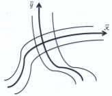
Figure 5: New coordinates.

In the new coordinates the function $E$ has the form

$$E=-\omega_{0}\bar{y}\bar{x}(1+O(|\bar{y}|+|\bar{x}|)),\quad\omega_{0}=\omega_{0}(z)>c_{2}^{-1}.\ \ \$$

Lemma 4.1

For $z\in B-c_{1}^{-1},\ |\bar{y}|<c_{3}^{-1},|\bar{x}|<c_{3}^{-1}$ there exists a smooth transformation of variables $\bar{F}\colon y,x,z\to\bar{y},\bar{x},z$ such that $\bar{y}=y+O(\varepsilon),\ \bar{x}=x+O(\varepsilon)$, and in the variables $y,x$ the perturbed motion is described by equations

$$\dot{x}=-\omega_{0}x(1+O(\varepsilon+|x|+|y|)),\ \dot{y}=\omega_{0}y(1+O(\varepsilon+|x|+|y|)).\ \$$

This Lemma is a direct corollary of a theorem by N. Fenichel (see [12], Theorem $11.1$). Coordinates of such type as $y,x$ here are often called Fenichel’s coordinates.

Lemma 4.1 allows to define in the domain $|\bar{y}|<c_{3}^{-1},|\bar{x}|<c_{3}^{-1}$ the transformation of variables $F\colon y,x\to p,q$ depending on $z$ as a parameter. The inverse transformation $F^{-1}\colon p,q\to y,x$ is defined in the $c_{4}^{-1}$-neighbourhood of the point $C$ in the plane $q,p$.

4.2 Lemmas on perturbed motion

Consider in the plane $x,y$ a square ${\cal K}=\{x,y\colon|x|<2c_{6}\sqrt{\varepsilon},\ |y|<2c_{6}\sqrt{\varepsilon},\}$. The constant $c_{6}$ is chosen below in Lemma 4.2 and Subsection 4.3.

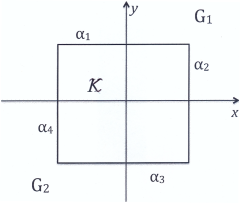
Figure 6: The square ${\cal K}$.

Let $\alpha_{1},...\alpha_{4}$ be sides of this square, the numeration of the sides corresponds to Fig. 6. Denote $\tilde{\cal{K}}=\tilde{\cal{K}}(z)=F[{\cal{K}}],\ \tilde{\alpha}_{i}=\tilde{\alpha}_{i}(z)=F[\alpha_{i}],\ i=1,...,4$. For a point $(p(t),q(t))$, that belongs to $c_{4}^{-1}$-neighbourhood of the point $C$, we denote $(y(t),x(t))=F^{-1}(p(t),q(t))$. The following two Lemmas show that points that started to move at sides of the square $\tilde{\cal{K}}$ far from its corners and not too close to the $x$-axis, will return to the sides of $\tilde{\cal{K}}$. In Fig. 7 the trajectories I and II correspond to Lemmas 4.2 and 4.3, respectively.

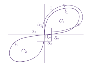
Figure 7: Trajectories I and II.

Lemma 4.2

If $z(t^{\prime})\in B-2c_{1}^{-1},\ (p(t^{\prime}),q(t^{\prime}))\in\tilde{\alpha}_{i}(z(t^{\prime})),i=1,3,\ |x(t^{\prime})|<c_{6}\sqrt{\varepsilon}$, then there exists a moment of time $t^{\prime\prime}$ such that

$$(p(t^{\prime\prime}),q(t^{\prime\prime}))\in\tilde{\alpha}_{i+1}(z(t^{\prime\prime})),\ t^{\prime\prime}-t^{\prime}=O(\ln\varepsilon),\ \ h(t^{\prime})-h(t^{\prime\prime})>c_{7}^{-1}\varepsilon\,.\$$

Remark. If we increase the value of the constant $c_{6}$, it would result in increasing of values of the constants $c_{j},\,j>7$. The constant $c_{7}$ can be chosen independently of $c_{6}$.

Lemma 4.3

Let $z(t^{\prime})\in B-2c_{1}^{-1},\ (p(t^{\prime}),q(t^{\prime}))\in\tilde{\alpha}_{2}(z(t^{\prime}))\cup\tilde{\alpha}_{4}(z(t^{\prime})),\ |y(t^{\prime})|>\varepsilon^{r_{1}}$, where $r_{1}$ is any given in advance positive number. If $(p(t^{\prime}),q(t^{\prime}))\in\tilde{\alpha}_{2}(z(t^{\prime})),\ y(t^{\prime})>\varepsilon^{r_{1}}$, then there exists a moment of time $t^{\prime\prime}$ such that

$$(p(t^{\prime\prime}),q(t^{\prime\prime}))\in\tilde{\alpha}_{1}(z(t^{\prime\prime})).$$

In analogous way,

$$\mbox{if}\ (p(t^{\prime}),q(t^{\prime}))\in\tilde{\alpha}_{2}(z(t^{\prime})),\ y(t^{\prime})<-\varepsilon^{r_{1}},\ \mbox{then}\ (p(t^{\prime\prime}),q(t^{\prime\prime}))\in\tilde{\alpha}_{3}(z(t^{\prime\prime})),\$$

$$\mbox{if}\ (p(t^{\prime}),q(t^{\prime}))\in\tilde{\alpha}_{4}(z(t^{\prime})),\ y(t^{\prime})>\varepsilon^{r_{1}},\ \mbox{then}\ (p(t^{\prime\prime}),q(t^{\prime\prime}))\in\tilde{\alpha}_{1}(z(t^{\prime\prime})),\phantom{**}\$$

$$\mbox{if}\ (p(t^{\prime}),q(t^{\prime}))\in\tilde{\alpha}_{4}(z(t^{\prime})),\ y(t^{\prime})<-\varepsilon^{r_{1}},\ \mbox{then}\ (p(t^{\prime\prime}),q(t^{\prime\prime}))\in\tilde{\alpha}_{3}(z(t^{\prime\prime})).\ \$$

In all cases $t^{\prime\prime}-t^{\prime}=O(\ln\varepsilon),\ h(t^{\prime\prime})-h(t^{\prime})=O(\varepsilon^{3/2})$.

The following assertion shows that a phase point that stared to move from a diagonal of the square $\tilde{\cal{K}}$ not too close to the origin of the coordinate system will arrive to a side of $\tilde{\cal{K}}$.

Lemma 4.4

If $z(t^{\prime})\in B-2c_{1}^{-1},\ (p(t^{\prime}),q(t^{\prime}))\in\tilde{\cal{K}}(z(t^{\prime})),\ y(t^{\prime})=-x(t^{\prime})>\varepsilon$, then there exists a moment of time $t^{\prime\prime}$ such that

$$(p(t^{\prime\prime}),q(t^{\prime\prime}))\in\tilde{\alpha}_{1}(z(t^{\prime\prime})),\ \ t^{\prime\prime}-t^{\prime}=O(\ln\varepsilon),\ h(t^{\prime\prime})-h(t^{\prime})=O(\varepsilon^{3/2}).\ \$$

Solutions of the averaged system with initial conditions from $W^{\delta}$ at $\tau=0$ cross the separatrix at $\tau,z$ such that $|\tau-\hat{\tau}_{*}|<c_{8}\delta,\ |z-\hat{z}_{*}|<c_{9}\delta$. Consider the surface $\Lambda$ in the space $x,y,z$:

$$\Lambda=\{x,y,z\colon|x|=2c_{6}\sqrt{\varepsilon},\ |z-\hat{z}_{*}|<2c_{9}\delta,\ |y|<\varepsilon^{r_{1}}\}.$$

Let $\tilde{\Lambda}$ be the image of this surface under the map $x,y,z\mapsto p,q,z$. Denote $\Xi$ the set in the space $p,q,z$ sweept by $\tilde{\Lambda}$ during the shift along the trajectories of the perturbed system (2.1) for time $t\in(-\hat{\tau}_{*}-2c_{8}\delta,-\hat{\tau}_{*}+2c_{8}\delta)$ before the first arrival to the boundary of the region $D-c_{1}^{-1}$.

Lemma 4.5

$$\mbox{\rm mes}\,\,\Xi=O(\varepsilon^{r_{1}-1/2}\mbox{\rm mes}\,W^{\delta}).$$

These Lemmas are proved in Subsections 4.4.2, 4.4.3

4.3 Proof of Proposition 2.3

Define $r_{1}=r+1/2$, where $r$ is the integer number introduced before the formulation of Theorem 1. Introduce $w=W^{\delta}\cap\Xi,\ W_{3}^{\delta}=W^{\delta}\setminus w$, where $\Xi$ is defined at the end of Subsection 4.2. According to Lemma 4.5 $\mbox{\rm mes}\,w=O(\varepsilon^{r}\mbox{mes}\,W^{\delta})$. Consider motion of a phase point $(p(t),q(t),z(t))$ that starts in $W_{3}^{\delta}$ at the moment of time $t=0$. In accordance with Proposition 2.1 the moment of time $t_{-}$ is defined such that $h(t_{-})=2k_{1}\varepsilon$. Then there exists a moment of time $t^{\prime}_{-}$ preceding $t_{-}$ such that the point $(p(t^{\prime}_{-}),q(t^{\prime}_{-}))$ lies in the $c_{4}^{-1}$-neighbourhood of the saddle $C$ for $z=z(t^{\prime}_{-})$, and $y(t^{\prime}_{-})=-x(t^{\prime}_{-})>0$, $c_{5}\varepsilon<h(t^{\prime}_{-})<2c_{5}\varepsilon$. The proof of the last assertion is completely analogous to the proofs of Lemmas 3.5, 3.6 and is omitted here.

Now let us choose the constant $c_{6}$ that defines the size of the square ${\cal{K}}$ in Subsection 4.2 (here we use the Remark to Lemma 4.2, which allows to increase the value of $c_{6}$). Choose $c_{6}$ such that in the segments $\alpha_{1}$ and $\alpha_{3}$ the inequality $-2k_{2}\varepsilon<E<4c_{5}\varepsilon$ implies the inequality $|x|<c_{6}\sqrt{\varepsilon}$ for $z\in B-c_{1}^{-1}$. In the segments $\alpha_{1}$ and $\alpha_{3}$ according to Lemma 4.1 we have $|E|=2\omega_{0}c_{6}\sqrt{\varepsilon}\,|x|+O(\varepsilon^{3/2}),\ \omega_{0}>c_{2}^{-1}$. Choose $c_{6}^{2}>4c_{2}\max(2c_{5},k_{2})$. Then for $|x|>c_{6}\sqrt{\varepsilon}$ we have $|E|>\max(4c_{5}\varepsilon,2k_{2})$. So, this choice of $c_{6}$ meets our condition. It is easy to check that under the same choice of $c_{6}$ the inequality $|E|>2c_{5}\varepsilon$ is satisfied on the line $x=-y$ outside of ${\cal{K}}$.

Let us return to the motion of the point $(p(t),q(t),z(t))$. It is evident that $y(t^{\prime})>\varepsilon$ (otherwise $h(t^{\prime})=O(\varepsilon^{2})<c_{5}\varepsilon$). In accordance with Lemma 4.4 there exists a moment of time $t^{\prime\prime}_{-}=t^{\prime}_{-}+O(\ln\varepsilon)$ such that $(p(t^{\prime\prime}_{-}),q(t^{\prime\prime}_{-}))\in\tilde{\alpha}_{1}(z(t^{\prime\prime}_{-}))$ and $h(t^{\prime\prime}_{-})=h(t^{\prime}_{-})+O(\varepsilon^{3/2})$. In particular $\frac{1}{2}c_{5}\varepsilon<h(t^{\prime\prime}_{-})<3c_{5}\varepsilon$ and, therefore, $|x(t^{\prime\prime}_{-})|<c_{6}\sqrt{\varepsilon}$ due to the choice of $c_{6}$. Now Lemmas 4.2, 4.3 allow, while their hypotheses are satisfied, to definite inductively the moments of time $t_{s}$ of consecutive arrivals of our phase point to the sides $\tilde{\alpha}_{1}$ or $\tilde{\alpha}_{3}$ of the square;  $t_{1}=t^{\prime\prime}_{-}$. In accordance with Lemmas 4.2, 4.3, $h(t_{s})-h(t_{s+1})>\frac{1}{2}c_{7}^{-1}\varepsilon$. As $|E|<c_{10}\sqrt{\varepsilon}$ in the square ${\cal{K}}$, so $s<4c_{7}c_{10}$. As $t_{s+1}-t_{s}=O(\ln\varepsilon)$, so $z(t_{s})-z(t_{1})=O(\ln\varepsilon)$ and, therefore, $z(t_{s})\in B-\frac{5}{2}c_{1}^{-1}$. If $|x(t_{s})|<c_{6}\sqrt{\varepsilon}$, then the moment of time $t_{s+1}$ do exists (here we use the following: because of the choice of initial conditions and the definition of the set $w$, the hypothesis $|y|>\varepsilon^{r_{1}}$ of Lemma 4.3 can not be violated). But the sequence $\{t_{s}\}$ should be finite: $s<4c_{7}c_{10}$. Therefore, there exists a number $s_{*}$ such that $|x(t_{s_{*}})|\geq c_{6}\sqrt{\varepsilon}$. Then because of the choice of $c_{6}$ it should be $h(t_{s_{*}})<-k_{2}\varepsilon$. By continuity there exists a moment of time $t_{+}\in(t_{-},t_{s_{*}})$ such that $h(t_{+})=-k_{2}\varepsilon$, as it was stated in Proposition 2.3.

Estimate $h(t),H_{\nu}(\varepsilon t),z(t),Z_{\nu}(\varepsilon t)$ for $t_{-}\leq t\leq t_{+}$. For $t\in(t_{-},t_{+})$ we have $h(t)=O(\varepsilon)$ by definitions of $t_{-},t_{+}$. As $H_{\nu}(\varepsilon t_{-})=O(\varepsilon),\ t_{+}-t_{-}=O(\ln\varepsilon)$ and, in correspondence with estimates of Lemmas 3.2, 3.3, $\dot{H}_{\nu}=O(\varepsilon/\ln|H_{\nu}|)\ \mbox{for}\ H_{\nu}\neq 0,\ \mbox{so}\ H_{\nu}(\varepsilon t)=O(\varepsilon)\ \mbox{for}\ t\in(t_{-},t_{+})$. As $\dot{z}=O(\varepsilon),\dot{Z}_{\nu}=O(\varepsilon)$, so for $t\in(t_{-},t_{+})$ we have

$$z(t)-Z_{\nu}(\varepsilon t)=O(\varepsilon\ln\varepsilon).$$

Improve the last estimate. From identity (3.3) we get

$$\dot{z}-\dot{Z}_{\nu}=\varepsilon O(|z-Z_{\nu}|)+\varepsilon O(1/\ln|H_{\nu}|)+\varepsilon f_{3}^{0}(p,q,z)-f_{3C}^{0}(z)+O(\varepsilon^{2}),\ \$$

where $f_{3C}^{0}$ is the value of the function $f_{3}^{0}(p,q,z)$ at the point $C$. Calculate integrals of the left and right sides of this relation with respect to time from $t_{s}$ to some $t\in(t_{s},t_{s+1})$. Making use of already established estimates for $H_{\nu},\ z-Z_{\nu}$, we get

$$z(t)-Z_{\nu}(\varepsilon t)=z(t_{s})-Z_{\nu}(\varepsilon t_{s})+O(\varepsilon)+\varepsilon\int_{t_{s}}^{t}(f_{3}^{0}(p,q,z)-f_{3C}^{0}(z))dt.\ \$$

The integrand in the last integral vanishes at the point $C$. Analogously to Lemma 3.5, this integral is $O(1)$. Therefore, for $t\in(t_{s},t_{s+1})$ we have

$$z(t)-Z_{\nu}(\varepsilon t)=z(t_{s})-Z_{\nu}(\varepsilon t_{s})+O(\varepsilon).\ \$$

Analogous estimate holds for $t_{1}\leq t\leq t_{-}\,$. As $s<4c_{7}c_{9}$ and, in accordance with Proposition 2.1, $z(t_{-})-Z_{\nu}(\varepsilon t_{-})=O(\varepsilon),\ \mbox{so}\ z(t)-Z_{\nu}(\varepsilon t)=O(\varepsilon)\ \mbox{for}\ t_{-}\leq t\leq t_{+}$. This was the assertion of Proposition 2.3.

Remark. In the proof of the last estimate the representation (3.3) was used. We can not use this representation in problems, where separatrices connect different saddle points, and at these points the function $f_{3}^{0}(p,q,z)$ has different values. The accuracy of description of $z$ in these cases is, in general, given by proved above estimate $z(t)-Z_{\nu}(\varepsilon t)=O(\varepsilon\ln\varepsilon)$ (see also Remark at the end of Subsection 3.3, part III).

4.4 Proofs of Lemmas on motion in a narrow vicinity of separatrices

4.4.1 Proof of Lemma 4.2

Let, for certainty, $(p(t^{\prime}),q(t^{\prime}))\in\tilde{\alpha}_{1}(z(t^{\prime}))$. Then for any choice of $c_{6}$ there exists a moment of time $t^{\prime\prime}>t^{\prime},\ t^{\prime\prime}=t^{\prime}+O(\ln\varepsilon)$ such that the point $(p(t^{\prime\prime}),q(t^{\prime\prime}))$ lies in the $c_{4}^{-1}$-neighbourhood of the saddle $C$, and $|x(t^{\prime\prime})|=2c_{6}\sqrt{\varepsilon},\ h(t^{\prime\prime})=h(t^{\prime})-\varepsilon\Theta_{2}(z(t^{\prime}))+O(\varepsilon^{3/2})$. The proof of this assertion is analogous to the proof of Lemma 3.5, and we omit it. Last estimate shows, in particular, that $c_{7}^{-1}\varepsilon\leq h(t^{\prime})-h(t^{\prime\prime})\leq d_{1}\varepsilon$, where $c_{7}$ and $d_{1}$ do not depend on choice of $c_{6}$. As $h(t^{\prime})=O(\varepsilon)$, so $h(t^{\prime\prime})=O(\varepsilon)$ and, therefore, $y(t^{\prime\prime})=O(\sqrt{\varepsilon})$. Now

$$h(t^{\prime})=-2\omega_{0}c_{6}\sqrt{\varepsilon}x(t^{\prime})+O(\varepsilon^{3/2}),\$$

$$h(t^{\prime\prime})=-2\omega_{0}c_{6}\sqrt{\varepsilon}y(t^{\prime\prime})+O(\varepsilon^{3/2}).\ \$$

From here

$$y(t^{\prime\prime})-x(t^{\prime})=\frac{h(t^{\prime})-h(t^{\prime\prime})}{2\omega_{0}c_{6}\sqrt{\varepsilon}}+O(\varepsilon).\ \$$

Choose $c_{6}^{2}>d_{1}c_{2}$. Then

$$|y(t^{\prime\prime})-x(t^{\prime})|<\frac{d_{1}c_{2}}{2}\frac{\sqrt{\varepsilon}}{c_{6}}+O(\varepsilon)<\frac{1}{2}c_{6}\sqrt{\varepsilon}+O(\varepsilon)<c_{6}\sqrt{\varepsilon}.$$

Therefore, if $|x(t^{\prime})|<c_{6}\sqrt{\varepsilon}$, then $|y(t^{\prime\prime})|<2c_{6}\sqrt{\varepsilon}$. This means that $(p(t^{\prime\prime}),q(t^{\prime\prime}))\in\tilde{\alpha}_{2}(z(t^{\prime\prime}))$. This was the assertion of the Lemma 4.2.

4.4.2 Proofs of Lemmas 4.3, 4.4

Let, for certainty, $(p(t^{\prime}),q(t^{\prime}))\in\tilde{\alpha}_{2}(z(t^{\prime})),\ y(t^{\prime})>\varepsilon^{r_{1}}$. Denote $t^{\prime\prime}$ the supremum of the moments of time $\bar{t}$ such that for $t^{\prime}\leq t\leq\bar{t}$ the following conditions hold:

$$z(t)\in B-c_{1}^{-1},\ -2c_{6}\sqrt{\varepsilon}\leq x(t)\leq 2c_{6}\sqrt{\varepsilon}+\varepsilon,\,\frac{1}{2}\varepsilon^{r_{1}}\leq y(t)\leq 2c_{6}\sqrt{\varepsilon}\,.$$ (4.1)

According to Lemma 4.1, for $t^{\prime}\leq t\leq t^{\prime\prime}$ we have $\dot{y}>\frac{1}{2}c_{2}^{-1}y$. Therefore $t^{\prime\prime}-t^{\prime}=O(\ln\varepsilon)$ and $z(t^{\prime\prime})\in B-\frac{3}{2}c_{2}^{-1}$. Then, again in correspondence with Lemma 4.1, on the segment $x=2c_{6}\sqrt{\varepsilon},\ |y|<2c_{6}\sqrt{\varepsilon}$ we have $\dot{x}<-c_{6}c_{2}^{-1}\sqrt{\varepsilon}$. On the segment $x=-2c_{6}\sqrt{\varepsilon},\ |y|<2c_{6}\sqrt{\varepsilon}$ we have $\dot{x}>c_{6}c_{2}^{-1}\sqrt{\varepsilon}$. Therefore, for $t^{\prime}\leq t\leq t^{\prime\prime}$ conditions for $x(t)$ in (4.1) hold as strict inequalities, and $|x(t^{\prime\prime})|<2c_{6}\sqrt{\varepsilon}$. In correspondence with the estimate $\dot{y}>\frac{1}{2}c_{2}^{-1}y$ we have $y(t^{\prime\prime})>\varepsilon^{r_{1}}$. As at the moment $t=t^{\prime\prime}$ the phase point should arrive to the boundary of the domain defined in (4.1), there exists the only possibility: $y(t^{\prime\prime})=2c_{6}\sqrt{\varepsilon}$, i.e. $(p(t^{\prime\prime}),q(t^{\prime\prime}))\in\tilde{\alpha}_{1}(z(t^{\prime\prime}))$.

In accordance with Lemma 4.1 for $t^{\prime}\leq t\leq t^{\prime\prime}$ we have

$$h(t)=-\omega_{0}(z(t))y(t)x(t)+O(\varepsilon^{3/2}),\ \frac{d}{dt}(\omega_{0}(z(t))y(t)x(t))=O(\varepsilon^{2}+|x|^{3}+|y|^{3})\,.\$$

Therefore, $h(t^{\prime\prime})-h(t^{\prime})=O(\varepsilon^{3/2})$, and this was the assertion of Lemma 4.3.

The proof of Lemma 4.4 follows the same lines.

4.4.3 Proof of Lemma 4.5

Denote $\tilde{\Lambda}\circ t$ the time-$t$ schift of the set $\tilde{\Lambda}$ along trajectories of the perturbed system (2.1). Denote $\tilde{\Lambda}\circ[a_{1},a_{2}]=\cup_{\begin{subarray}{c}t\in[a_{1},a_{2}]\end{subarray}}\tilde{\Lambda}\circ t$. Assume for simplicity of explanation that $\tilde{\Lambda}\circ[-K/\varepsilon,0]\in D$ (it is easy to avoid this restriction by considering only the part of the set $\tilde{\Lambda}\circ[-K/\varepsilon,0]$ which does not leave $D$). For the set $\Xi$ we have

$$\Xi=\left(\tilde{\Lambda}\circ\left[\frac{-\hat{\tau}_{*}-2c_{8}\delta}{\varepsilon},\frac{-\hat{\tau}_{*}+2c_{8}\delta}{\varepsilon}\right]\right)\cap(D-c_{1}^{-1}).$$

Consider $\Xi_{0}=\tilde{\Lambda}\circ[-d_{1}^{-1},0]$. For small enough $d_{1}^{-1}$ the points of this set lie in $B-\frac{3}{2}c_{1}^{-1}$ with respect to $z$ and in $\frac{1}{2}c_{4}^{-1}$-neighbourhood of the saddle point $C$ with respect to $(p,q)$. Therefore the set $\Xi_{0}$ can be considered in the variables $x,y,z$ of Lemma 4.1. As in these variables the phase flux through $\tilde{\Lambda}$ is $O(\varepsilon^{r_{1}+1/2}\delta^{l-2})$, so the phase volume of the set $\Xi_{0}$ is $O(\varepsilon^{r_{1}+1/2}\delta^{l-2})$, if the volume element is $dxdydz$. As the Jacobian of the transformation $x,y,z\mapsto p,q,z$ is $O(1)$, so the same estimate of the phase volume is valid if the volume element is $dpdqdz$. Consider now sets

$$\Xi_{j} = \Xi_{0}\circ(-jd_{1}^{-1}),\$$

$$j = \left[\frac{(\hat{\tau}_{*}-2c_{8}\delta)d_{1}}{\varepsilon}\right]-1,...,\left[\frac{(\hat{\tau}_{*}+2c_{8}\delta)d_{1}}{\varepsilon}\right]+1.\$$

We have mes $\Xi_{j}=O(\mbox{mes}\,\,\Xi_{0})$, as the divergence of the right hand side of system (2.1) is $O(\varepsilon)$, and so the distortion of the phase volume in this system during the time $O(1/\varepsilon)$ does not exceed $O(1)$ times. As $\Xi\subset\cup_{\begin{subarray}{c}j\end{subarray}}\,\Xi_{j}$, we get mes $\Xi=O(\varepsilon^{r_{1}-1/2}\delta^{l-1})=O(\varepsilon^{r_{1}-1/2}\mbox{mes}\,W^{\delta})$. Lemma 4.5 is proved.

5 Calculation of measures captured into different regions at the separatrix

In this section Propositions 2.4 and 2.5 of Subsection 2.5 are proved.

5.1 Preliminary constructions

Denote $I=I(\nu,z,h)$ the value of the action variable for the trajectory $E=h$ of the unperturbed system in the region $G_{\nu},\ \nu=1,2,3$. Since in each of the regions $G_{\nu}$ the dependence of $I$ on $h$ is monotonous, we can rewrite in any $G_{\nu}$ the averaged system (2.3) as a system of differential equations for $I,z$. Making use of gluing of solutions of averaged system at the separatrix (see Subsection 2.3), we can consider the averaged system with respect to the variable $\gamma=(\nu,z,I)$. Separatrix crossing leads to a jump of values $\nu$ and $I$. Denote $\bar{g}_{1}^{\tau}(\gamma)$ the shift of the point $\gamma$ for slow time $\tau=\varepsilon t$ along the trajectory of such averaged system, $\bar{g}_{1}^{0}(\gamma)=\gamma$, and index “1” indicates that the solutions with $\nu=3$ and $\nu=1$ are glued at the separatrix. Denote $W=W^{\delta},\ W_{\nu}=W_{\nu}^{\delta},\ \alpha=(p,q,z)$. Let $\Pi(\cdot)$ be the standard projection from the $\alpha$-space to the $\gamma$-space; $\Pi(\alpha)=\gamma$. Denote

$$\Gamma=\Pi[W],\ \Gamma_{1}^{K}=\bar{g}_{1}^{K}[\Gamma],W_{1}^{K}=\Pi^{-1}[\Gamma_{1}^{K}].$$

We will denote points from $\Gamma,\Gamma_{1}^{K},W,W_{1}^{K}$ as $\gamma^{0},\gamma^{K},\alpha^{0}=(p^{0},q^{0},z^{0}),\alpha^{K}=(p^{K},q^{K},z^{K})$ respectively.

5.2 Proof of the Proposition 2.4

Denote $g^{t}(\alpha)$ the time-$t$ shift of a point $\alpha=(p,q,z)$ along the trajectory of system (2.1). Consider $g^{t}(\alpha^{K})$ for $\alpha^{K}\in W_{1}^{K}$. Estimates in Propositions 2.1, 2.2, 2.3 were proved for initial conditions from $W$. Analogous estimates are valid for initial conditions from $W_{1}^{K}$, if we consider the motion in reverse direction in time. From this we get the following assertion: there exists a set $w_{1}\subset W_{1}^{K},\ \mbox{mes}\ w_{1}=O(\varepsilon^{r}\delta^{l-1})$, such that for initial conditions $\alpha^{K}\in W_{1}^{K}\setminus w_{1}$ the behaviour of $h,z$ along $g^{t}(\alpha^{K}),\ -K\varepsilon\leq t\leq 0$, is described with an accuracy $O(\varepsilon\ln\varepsilon)$ by the solution of averaged system glued of solutions in $G_{1}$ and $G_{3}$ (passage from $G_{1}$ to $G_{2}$ is impossible for $\alpha^{K}\in W_{1}^{K}\setminus w_{1}$). It follows from these estimates that there exists a set ${W^{\prime}}_{1}^{K}\subseteq W_{1}^{K}$ such that $g^{-K\varepsilon^{-1}}[{W^{\prime}_{1}}^{K}]\subseteq W,\ \mbox{mes}\,(W_{1}^{K}\setminus{W^{\prime}_{1}}^{K})=O(\varepsilon\ln\varepsilon\,\,\delta^{l-2})$. Denote $W^{\prime}_{1}=g^{-K\varepsilon^{-1}}[{W^{\prime}_{1}}^{K}]$. The definition of $W_{2}$ implies that

$$W^{\prime}_{1}\subseteq W\setminus W_{2}=W_{1}\cup w$$

A standard calculation of change of a phase volume along a motion gives us

$$\mbox{mes}\,W^{\prime}_{1}=\int\limits_{{W^{\prime}_{1}}^{K}}\exp\left(-\varepsilon\int\limits_{0}^{K\varepsilon^{-1}}\left(\frac{\partial f_{1}}{\partial q}+\frac{\partial f_{2}}{\partial p}+\frac{\partial f_{3}}{\partial z}\right)dt\right)dp^{K}dq^{K}dz^{K}.\$$ (5.1)

Here the outer integral is calculated with respect to initial (or, better to say, “final”) conditions from the set ${W^{\prime}_{1}}^{K}$. The inner integral is calculated with respect to time along a solution of system (2.1) with given “final” condition. In the integral with respect to time it is reasonable to replace exact solution with the averaged one $\bar{g}_{1}^{-\tau}(\gamma^{K})$, and to estimate the accuracy of this approximation. The result is described by the following Lemma, which is proved in Subsection 5.4.1.

Lemma 5.1

For $\alpha^{K}\in{{W^{\prime}_{1}}^{K}}$ the following estimate holds:

$$\varepsilon\int\limits_{0}^{K\varepsilon^{-1}}\left(\frac{\partial f_{1}}{\partial q}+\frac{\partial f_{2}}{\partial p}+\frac{\partial f_{3}}{\partial z}\right)dt=\int\limits_{0}^{K}{\cal F}(\bar{\gamma})d\tau+O(\varepsilon\ln\varepsilon),$$

$$\mbox{\rm where}\ \bar{\gamma}=\bar{g}_{1}^{-\tau}(\gamma^{K}),\ \gamma^{K}=\Pi(\alpha^{K}),$$

$${\cal F}(\gamma)=\frac{1}{T}\oint\limits_{\gamma}\left(\frac{\partial f_{1}^{0}}{\partial q}+\frac{\partial f_{2}^{0}}{\partial p}+\frac{\partial f_{3}^{0}}{\partial z}\right)dt.\$$

The integral with index $\gamma=(\nu,Z,J)$ is calculated along the level line of the Hamiltonian $E$ in the region $G_{\nu}(z)$, and the “action” for this level line is equal to $J$. The parameter along the level line is time $t$ of the unperturbed motion, $T$ is the period of this motion.

Making use of Lemma 5.1 we get

$$\mbox{mes}\ W_{1}^{\prime}=\int\limits_{{W_{1}^{\prime}}^{K}}\exp\left(-\int\limits_{0}^{K}{\cal F}(\bar{\gamma})d\tau\right)dp^{K}dq^{K}dz^{K}+O(\varepsilon\ln\varepsilon\ \delta^{l-2}).\ \$$

Replace domain of integration ${W_{1}^{\prime}}^{K}$ with $W_{1}^{K}$ in the last expression. This gives an additional error $O(\varepsilon\ln\varepsilon\ \delta^{l-2})$. We get

$$\mbox{mes}\ W_{1}^{\prime}=\int\limits_{W_{1}^{K}}\exp\left(-\int\limits_{0}^{K}F(\bar{\gamma})d\tau\right)dp^{K}dq^{K}dz^{K}+O(\varepsilon\ln\varepsilon\ \delta^{l-2}).\ \$$

In the last expression we can use action-angle variables $J^{K},\varphi^{K}$ instead of $p^{K},q^{K}$ as independent variables. As integrand does not depend on $\varphi^{K}$, we get

$$\mbox{mes}\ W_{1}^{\prime}=2\pi\int\limits_{\Gamma_{1}^{K}}\exp\left(-\int\limits_{0}^{K}{\cal{F}}(\bar{\gamma})d\tau\right)dJ^{K}dz^{K}+O(\varepsilon\ln\varepsilon\ \delta^{l-2}).\ \$$

Let us make in the outer integral the transformation of variables $(J^{K},z^{K})\mapsto(J^{0},z^{0})$ by means of the formula $\bar{g}_{1}^{K}(\gamma^{0})=\gamma^{K}$, where $\gamma^{0}=(3,z^{0},J^{0}),\ \gamma^{K}=(1,z^{K},J^{K})$. We get

$$\mbox{mes}\ (W_{1}^{\prime})=2\pi\int\limits_{\Gamma}\Omega_{0,K}(\gamma^{0})dJ^{0}dz^{0}+O(\varepsilon\ln\varepsilon\ \delta^{l-2}),\ \$$

where

$$\Omega_{0,K}(\gamma^{0})=\exp\left(-\int\limits_{0}^{K}{\cal{F}}(\bar{\gamma})d\tau\right)\frac{\partial(J^{K},z^{K})}{\partial(J^{0},z^{0})},\quad\bar{\gamma}=\bar{g}_{1}^{\tau}(\gamma^{0}).$$

Lemma 5.2

$$\Omega_{0,K}(\gamma^{0})=P_{1}(z_{*})=\Theta_{1}(z_{*})/\Theta_{3}(z_{*}),$$

where $z_{*}=z_{*}(\gamma^{0})$ is the value of $z$ at the moment of the separatrix crossing for the solution of averaged system $\bar{g}_{1}^{\tau}(\gamma^{0})$.

This Lemma is proved in Subsection 5.4.2.

Because of Lemma 5.2

$$\mbox{mes}\ {W}_{1}^{\prime}=2\pi\int\limits_{\Gamma}P_{1}(z_{*})dJ^{0}dz^{0}+O(\varepsilon\ln\varepsilon\ \delta^{l-2}).\$$ (5.2)

As ${W}_{1}^{\prime}\subseteq W_{1}\cup w$ and $\mbox{mes}\ w=O(\varepsilon^{r}\ \delta^{l-1})$, so

$$\mbox{mes}\ W_{1}^{\prime}<\mbox{mes}\ W_{1}+O(\varepsilon^{r}\ \delta^{l-1}).$$

In completely analogous way, but for the index $\nu=2$, we get that there exists a set ${W}_{2}^{\prime}\subseteq W_{2}\cup w$ such that

$$\mbox{mes}\ {W}_{2}^{\prime} = 2\pi\int\limits_{\Gamma}P_{2}(z_{*})\,dJ^{0}dZ^{0}+O(\varepsilon\ln\varepsilon\ \delta^{l-2}),$$ (5.3)

$$\mbox{mes}\ {W}_{2}^{\prime} < \mbox{mes}\ W_{2}+O(\varepsilon^{r}\ \delta^{l-1}).$$

Consider relations

$$\mbox{mes}\ {W}_{1}^{\prime} < \mbox{mes}\ W_{1}+O(\varepsilon^{r}\ \delta^{l-1}),$$ (5.4)

$$\mbox{mes}\ {W}_{2}^{\prime} < \mbox{mes}\ W_{2}+O(\varepsilon^{r}\ \delta^{l-1}),$$

$$\mbox{mes}\ W_{1} + \mbox{mes}\ W_{2}=\mbox{mes}\ W+O(\varepsilon^{r}\ \delta^{l-1}),$$

$$\mbox{mes}\ {W}_{1}^{\prime} + \mbox{mes}\ {W}_{2}^{\prime}=\mbox{mes}\ W+O(\varepsilon\ln\varepsilon\ \delta^{l-2}).\$$

To get the last equality, it is enough to add (5.2) and (5.3), and to take into account that $P_{1}+P_{2}=1$. From (5.4) we get

$$\mbox{mes}\ W_{1} = \mbox{mes}\ W-\mbox{mes}\ W_{2}+O(\varepsilon^{r}\delta^{l-1})=\mbox{mes}\ {W}_{1}^{\prime}+\mbox{mes}\ {W}_{2}^{\prime}-\mbox{mes}\ W_{2}+O(\varepsilon\ln\varepsilon\delta^{l-2})\$$

$$< \mbox{mes}\ {W}_{1}^{\prime}+O(\varepsilon\ln\varepsilon\ \delta^{l-2}),\ \ \$$

and, on the other hand,

$$\mbox{mes}\ W_{1}>\mbox{mes}\ {W}_{1}^{\prime}+O(\varepsilon^{r}\ \delta^{l-1}).$$

Therefore we get

$$\mbox{mes}\ W_{1} = \mbox{mes}\ {W}_{1}^{\prime}+O(\varepsilon\ln\varepsilon\ \delta^{l-2})=2\pi\int\limits_{\Gamma}P_{1}(z_{*})\,dJ^{0}dz^{0}+O(\varepsilon\ln\varepsilon\ \delta^{l-2})=\$$

$$= \int\limits_{W}P_{1}(z_{*})dp^{0}dq^{0}dz^{0}+O(\varepsilon\ln\varepsilon\ \delta^{l-2}),\$$

and analogous expression for $W_{2}$. Proposition 2.4 is proved.

5.3 Proof of Proposition 2.5

Let $I,\varphi\ \mbox{mod}\ 2\pi$ be the action-angle variables of the system with Hamiltonian $E$ in a neighbourhood of the set $W^{\delta}$. Consider in system (2.1) variable $\varphi$ as a new time. For $I,z$ we get a nonautonomous system of $l-1$ equations. Consider for this system extended phase space with space variables $I,z,\varphi$ and a new time $\vartheta\colon d\vartheta/d\varphi=1$. Now for $\varphi,I,z$ we have

$$\varphi^{\prime}=1,\ I^{\prime}=\varepsilon f_{4},\ z^{\prime}=\varepsilon f_{5}\,.$$

Here “prime” denotes derivative with respect to $\vartheta,\ f_{i}=f_{i}(\varphi,I,z,\varepsilon),\ j=4,5$, are smooth functions. Denote $u^{\vartheta}$ the operator of the shift along the trajectories of this system during the time $\vartheta$. Consider the sequence of the sets

$$u^{2s\delta}(U^{\delta}),\ s=0,1,...,N-1,N=[\pi/\delta]\,.$$

Only adjoining sets in this sequence can intersect each other. The measure of any such intersection is $O(\varepsilon\delta^{l-1})$. Making use of the fact that the shift along the trajectories of this system during the time $O(1)$ distorts measure only with a coefficient $1+O(\varepsilon)$, we get

$$\mbox{mes}\ \bigcup\limits_{s=0}^{N-1}u^{2s\delta}(U^{\delta})=N\,\mbox{mes}\,U^{\delta}+O(\varepsilon\delta^{l-2}).$$ (5.5)

Analogous reasoning for sets $U_{\nu}^{\delta},\,\nu=1,2$, gives the estimate

$$\mbox{mes}\ \bigcup\limits_{s=0}^{N-1}u^{2s\delta}(U_{\nu}^{\delta})=N\,\mbox{mes}\,U_{\nu}^{\delta}+O(\varepsilon\delta^{l-2}).$$ (5.6)

Then

$$\mbox{mes}\ (W^{\delta}\!\!\vartriangle\!\bigcup\limits_{s=0}^{N-1}u^{2s\delta}(U^{\delta}))=O(\varepsilon\delta^{l-2}+\delta^{l}),$$ (5.7)

$$\mbox{mes}\ (W_{\nu}^{\delta}\!\!\vartriangle\!\bigcup\limits_{s=0}^{N-1}u^{2s\delta}(U_{\nu}^{\delta}))=O(\varepsilon\delta^{l-2}+\delta^{l}).\ \$$

Here it is taken into account that $u^{\vartheta}(U_{\nu}^{\delta})\cap W^{\delta}\subseteq W_{\nu}^{\delta}\cup w;\ \ \vartriangle$ is the symbol of symmetric difference of sets. From (5.5) - (5.7) we get

$$\mbox{mes}\ U^{\delta}=\frac{1}{N}\ \mbox{mes}\ W^{\delta}+O(\varepsilon\delta^{l-1}+\delta^{l+1}),$$

$$\mbox{mes}\ U_{\nu}^{\delta}=\frac{1}{N}\ \mbox{mes}\ W_{\nu}^{\delta}+O(\varepsilon\delta^{l-1}+\delta^{l+1}),\$$

$$\frac{\mbox{mes}\ U_{\nu}^{\delta}}{\mbox{mes}\ U^{\delta}}=\frac{\mbox{mes}\ W_{\nu}^{\delta}}{\mbox{mes}\ W^{\delta}}+O(\delta+\frac{\varepsilon}{\delta}).\ \$$

From here and from the result of Proposition 2.4 we get

$$\frac{\mbox{mes}\ U_{\nu}^{\delta}}{\mbox{mes}\ U^{\delta}}=\frac{\Theta_{\nu}(\hat{z}_{*})}{\Theta_{3}(\hat{z}_{*})}+O\left(\delta+\frac{\varepsilon|\ln\varepsilon|}{\delta}\right).\ \$$

This was the assertion of Proposition 2.5.

5.4 Proofs of Lemmas on measure estimates

5.4.1 Proof of Lemma 5.1

Denote

$$\chi=\chi(p,q,z,\varepsilon)=\frac{\partial f_{1}}{\partial q}+\frac{\partial f_{2}}{\partial p}+\frac{\partial f_{3}}{\partial z},\quad\chi^{0}=\chi(p,q,z,0).$$

We have

$$\varepsilon\int\limits_{0}^{K\varepsilon^{-1}}\chi dt = \varepsilon\int\limits_{0}^{K\varepsilon^{-1}}\chi^{0}dt+O(\varepsilon)$$

$$= \varepsilon\int\limits_{0}^{{t^{\prime}}_{-}}\chi^{0}dt+\varepsilon\int\limits_{{t^{\prime}}_{-}}^{{t^{\prime}}_{+}}\chi^{0}dt+\varepsilon\int\limits_{{t^{\prime}}_{+}}^{K\varepsilon^{-1}}\chi^{0}dt+O(\varepsilon),\$$

where ${t^{\prime}_{-}}$ and ${t^{\prime}_{+}}$ are the moments of the time analogous to the moments ${t_{-}},\ {t_{+}}$ introduced in Subsection 2.5, but for initial conditions from $W_{1}^{K}$. As ${t^{\prime}_{-}}-{t^{\prime}_{+}}=O(\ln\varepsilon)$, so the second term in the right hand side of the last equality is $O(\varepsilon\ln\varepsilon)$.

For $0\leq t\leq{t^{\prime}}_{-}$ we will consider motion round by round, as it was done in Section 3. Suppose for simplicity of the exposition that during any round the phase point crosses the ray $C\eta$ just one time, and that the motion takes place in the region $|E|<1/2$. Denote $t_{1}<t_{2}<...<t_{N}$ the successive moments of the crossing of $C\eta,\ t_{i}\in(0,{t^{\prime}}_{-})$. According to Lemma 3.5 and its Corollary, we have

$$\frac{\varepsilon}{t_{i+1}-t_{i}}\int\limits_{t_{i}}^{t_{i+1}}\chi^{0}dt=\frac{\varepsilon}{T(h(t_{i}),z(t_{i}))}\oint\limits_{E=h(t_{i})}\chi^{0}dt+\varepsilon^{2}O\left(h^{-1}(t_{i})\ln^{-1}h(t_{i})\right).$$ (5.9)

According to Propositions 2.1 - 2.3

$$|h(t_{i})-H_{1}(t_{i})|+|z(t_{i})-Z_{1}(t_{i})|=O\left(\frac{\varepsilon\ln\varepsilon}{\ln H_{1}(t_{i})}\right),$$ (5.10)

$$\frac{1}{2}H_{1}(t_{i})<h(t_{i})<2H_{1}(t_{i}).\phantom{************}\ \$$

From (5.9), (5.10), making use of Lemma 3.4 and estimate (4) of Lemma 3.2 we get

$$\frac{\varepsilon}{t_{i+1}-t_{i}}\int\limits_{t_{i}}^{t_{i+1}}\chi^{0}dt=\frac{\varepsilon}{T(H_{1}(t_{i}),Z_{1}(t_{i}))}\oint\limits_{\begin{subarray}{c}E=H_{1}(t_{i})\\ z=Z_{1}(t_{i})\end{subarray}}\chi^{0}dt+O\left(\frac{\varepsilon^{2}\ln\varepsilon}{H_{1}(t_{i})\ln^{3}H_{1}(t_{i})}\right).\ \$$

Let us multiplay the left and right hand sides of this equality by
$t_{i+1}-t_{i}=O(\ln H(t_{i}))$ and sum up the obtained estimates. Taking into account that $t_{1}=O(1),\ t_{N}={t^{\prime}}_{-}+O(\ln\varepsilon)$, we get

$$\varepsilon\int\limits_{0}^{t^{\prime}_{-}}\chi^{0}dt=\sum\limits_{i=1}^{N}\frac{1}{T(H_{1}(t_{i}),Z_{1}(t_{i}))}\,\,(\!\oint\limits_{\begin{subarray}{c}E=H_{1}(t_{i})\\ z=Z_{1}(t_{i})\end{subarray}}\chi^{0}dt\ \ )\ \varepsilon(t_{i+1}-t_{i})+O(\varepsilon\ln\varepsilon).\ \$$

The sum in the right hand side can be represented as an integral with an accuracy $O(\varepsilon\ln\varepsilon)$. Therefore, we have

$$\varepsilon\int\limits_{0}^{t_{-}^{\prime}}\chi^{0}dt=\int\limits_{0}^{\tau_{*}}{\cal{F}}(\bar{\gamma})d\tau+O(\varepsilon\ln\varepsilon),\ \$$

where $\tau_{*}$ is the moment of the separatrix crossing in the averaged system. In the analogous way

$$\varepsilon\int\limits_{{t^{\prime}}_{+}}^{K\varepsilon^{-1}}\chi^{0}dt=\int\limits_{\tau_{*}}^{K}{\cal{F}}(\bar{\gamma})d\tau+O(\varepsilon\ln\varepsilon).\ \$$

Results of Lemma 5.1 follow from these estimates and (5.4.1).

5.4.2 Proof of Lemma 5.2

Let $\tau_{3}$ and $\tau_{1}$ be any numbers such that $0\leq\tau_{3}<\tau_{*}<\tau_{1}\leq K$. Here $\tau_{*}=\tau_{*}(\gamma^{0})$ is the moment of the separatrix crossing for $\bar{g}_{1}^{\tau}(\gamma^{0})$. Denote

$$\bar{g}_{1}^{\tau_{3}}(\gamma^{0})=\gamma^{(3)}=(3,z^{(3)},J^{(3)}),\ \bar{g}_{1}^{\tau_{1}}(\gamma^{0})=\gamma^{(1)}=(1,z^{(1)},J^{(1)}).$$

Each of values $\gamma^{0},\gamma^{(3)},\gamma^{(1)},\gamma^{K}$ defines all others. These values can be defined also through $\tau_{*},z_{*}$. Denote

$$\Omega_{\tau_{3},\tau_{1}}=\exp\left(-\int\limits_{\tau_{3}}^{\tau_{1}}{\cal{F}}(\bar{\gamma})d\tau\right)\frac{\partial(J^{(1)},z^{(1)})}{\partial(J^{(3)},z^{(3)})}.\$$ (5.11)

Similarly define $\Omega_{0,\tau_{3}}$ and $\Omega_{\tau_{1},K}$. Then

$$\Omega_{0,K}=\Omega_{0,\tau_{3}}\Omega_{\tau_{3},\tau_{1}}\Omega_{\tau_{1},K}\,.$$

Lemma 5.3

$\Omega_{0,\tau_{3}}=1,\ \Omega_{\tau_{1},K}=1\,.$

This Lemma is proved in Subsection 5.4.3.

Corollary 5.1

$\Omega_{0,K}=\Omega_{\tau_{3},\tau_{1}}$ .

Now let $\tau_{3}$ and $\tau_{1}$ tend to $\tau_{*}$. The first multiplier in (5.11) tends to $1$. Therefore

$$\Omega_{0,K}=\lim_{\begin{subarray}{c}\tau_{3}\to\tau_{*}-0\\ \tau_{1}\to\tau_{*}+0\end{subarray}}\frac{\partial(J^{(1)},z^{(1)})}{\partial(J^{(3)},z^{(3)})}=\left.\lim_{\tau_{1}\to\tau_{*}+0}\frac{\partial(J^{(1)},z^{(1)})}{\partial(\tau_{*},z_{*})}\right/\lim_{\tau_{1}\to\tau_{*}-0}\frac{\partial(J^{(3)},z^{(3)})}{\partial(\tau_{*},z_{*})}\,.$$

Let us calculate these limits. Denote $F$ and $\Phi$ the right hand sides of the averaged equations for $I$ and $z$ respectively. Then

$$J^{(1)}=\frac{1}{2\pi}S_{1}(z_{*})+\int\limits_{\tau_{*}}^{\tau_{1}}Fd\tau\,,\quad z^{(1)}=z_{*}+\int\limits_{\tau_{*}}^{\tau_{1}}\Phi d\tau\,.\$$

Integrals here are calculated along the solution of the averaged system $\bar{g}_{1}^{\tau}(\gamma^{0})$, and $S_{1}=S_{1}(z)$ is the area of the region $G_{1}(z)$. Making use of the formulas for the right hand sides of averaged system (2.3), (2.7), we get

$$\lim_{\tau_{1}\to\tau_{*}+0}\frac{\partial J^{(1)}}{\partial\tau_{*}} = -\lim_{\tau_{1}\to\tau_{*}+0}F=\frac{1}{2\pi}\left(\Theta_{1}(z_{*})+\left(\oint\limits_{l_{1}}\frac{\partial E}{\partial z}dt\right)\,f_{3c}^{0}\right),$$

$$\lim_{\tau_{1}\to\tau_{*}+0}\frac{\partial z^{(1)}}{\partial\tau_{*}} = -\lim_{\tau_{1}\to\tau_{*}+0}\Phi=-f_{3c}^{0},$$

$$\lim_{\tau_{1}\to\tau_{*}+0}\frac{\partial J^{(1)}}{\partial z_{*}} = \frac{1}{2\pi}\frac{\partial S_{1}}{\partial z_{*}}=-\frac{1}{2\pi}\oint\limits_{l_{1}}\frac{\partial E}{\partial z}dt,$$

$$\lim_{\tau_{1}\to\tau_{*}+0}\frac{\partial z^{(1)}}{\partial z_{*}} = {\bf 1}_{l-2}.\$$

Here ${\bf 1}_{l-2}$ is the unit $(l-2)\times(l-2)$ matrix; $f_{3c}^{0}$ is the value of the function $f_{3}^{0}$ at the saddle point $C$ for $z=z_{*}$. Making use of these relations, we get

$$\lim_{\tau_{1}\to\tau_{*}+0}\frac{\partial(J^{(1)},z^{(1)})}{\partial(\tau_{*},z_{*})}=\begin{vmatrix}\frac{1}{2\pi}\left(\Theta_{1}(z_{*})+\left(\oint\limits_{l_{1}}\frac{\partial E}{\partial z}dt\right)\,f_{3c}^{0}\right),&-\frac{1}{2\pi}\oint\limits_{l_{1}}\frac{\partial E}{\partial z}dt\\ -f_{3c}^{0},&{\bf 1}_{l-2}\\ \end{vmatrix}=\frac{1}{2\pi}\Theta_{1}(z_{*})\,.\$$

Similarly,

$$\lim_{\tau_{3}\to\tau_{*}-0}\frac{\partial(J^{(3)},z^{(3)})}{\partial(\tau_{*},z_{*})}=\frac{1}{2\pi}\Theta_{3}(z_{*})\,.$$

Finally we have

$$\Omega_{0,K}=\Theta_{1}(z_{*})/\Theta_{3}(z_{*})\,.$$

This was the assertion of Lemma 5.2.

5.4.3 Proof of Lemma 5.3

To avoid long calculations with derivatives we will use known results about the averaging method. Denote $\Gamma_{0}$ a neighbourhood of the point $(3,z^{0},J^{0})$ such that $\bar{g}_{1}^{\tau}(\gamma)$ does not cross the separatrix for $0\leq\tau\leq\tau_{1}$ and $\gamma\in\Gamma_{0}$. Let $W_{0}=\Pi^{-1}(\Gamma_{0})$, where $\Pi$ is the standard projection from $p,q,z$-space to $\gamma=(\nu,z,J)$-space. The reasoning of the Subsection 5.1 shows that there exists a set $W^{\prime}_{0}\in W_{0}$ such that

$$\mbox{mes}\ {W_{0}}^{\prime} = \mbox{mes}\ W_{0}+O(\varepsilon),$$

$$\mbox{mes}\ {W_{0}}^{\prime} = 2\pi\int\limits_{\Gamma_{0}}\Omega_{0,\tau_{3}}dJ^{0}dz^{0}+O(\varepsilon).\$$

From here

$$\mbox{mes}\ {W_{0}}-2\pi\int\limits_{\Gamma_{0}}\Omega_{0,\tau_{3}}dJ^{0}dz^{0}=O(\varepsilon).$$

As the left hand side does not depend on $\varepsilon$, so

$$\mbox{mes}\ {W_{0}}=2\pi\int\limits_{\Gamma_{0}}\Omega_{0,\tau_{3}}dJ^{0}dz^{0}=\int\limits_{W_{0}}\Omega_{0,\tau_{3}}dp^{0}dq^{0}dz^{0}.$$

Therefore $\Omega_{0,\tau_{3}}=1$. Similarly, $\Omega_{\tau_{1},K}=1$. Lemma 5.3 is proved.

5.5 A rule for calculation of probabilities

A heuristic reasoning of [21, 14], which leads to the formulas of Section 2 for probabilities of capture into different regions, is exposed in this subsection. This reasoning can be used as, in some sense, a rule, as it allows to calculate probabilities in general case of systems of form (2.1), for other than in Fig. 2 types of phase portraits. This reasoning is justified by Proposition 5.1 of this subsection.

5.5.1 A scheme of calculation of probabilities

The following reasoning does not pretend to be rigorous. A corresponding rigorous assertion is formulated at the end of this subsection. Let $C\xi\eta=C\xi\eta(z)$ be the system of principal axes for the saddle point $C$ oriented as in Fig. 2. Let a phase point $(p(t),q(t))$ start moving at a moment of time $t=t^{\prime}$ with $z=z^{\prime},\ E=h^{\prime}$ from the ray $C\eta$. Denote $\Theta_{\nu}=\Theta_{\nu}(z^{\prime})$. The point $(p(t),q(t))$ first makes a curve $l_{2}^{\prime}$, which is close to $l_{2}(z)$. At the end of this curve

$$E=h^{\prime\prime}=h^{\prime}+\int\limits_{l^{\prime}_{2}}\frac{dE}{dt}dt\approx h^{\prime}+\int\limits_{l_{2}}\frac{dE}{dt}dt=h^{\prime}-\varepsilon\Theta_{2}\,.$$

If $0<h^{\prime}<\varepsilon\Theta_{2}$, then $h^{\prime\prime}<0$, i.e. the phase point is captured into the region $G_{2}$. If $h^{\prime}>\varepsilon\Theta_{2}$, then in further motion the phase point makes a curve $l^{\prime}_{1}$, which is close to $l_{1}(z^{\prime})$. At the end of this curve $E=h^{\prime\prime\prime}\approx h^{\prime}-\varepsilon(\Theta_{1}+\Theta_{2})$. If $\varepsilon\Theta_{2}<h^{\prime}<\varepsilon(\Theta_{1}+\Theta_{2})$, then $h^{\prime\prime\prime}<0$, i.e. the phase point is captured into the region $G_{1}$. If $h^{\prime}>\varepsilon(\Theta_{1}+\Theta_{2})$, then $h^{\prime\prime\prime}>0$, i.e. the phase point comes back to $C\eta$. Introduce intervals $\varkappa_{1}=(\varepsilon\Theta_{2},\ \varepsilon(\Theta_{1}+\Theta_{2})),\ \varkappa_{2}=(0,\varepsilon\Theta_{2},),\ \varkappa_{3}=(\varepsilon(\Theta_{1}+\Theta_{2}),\infty),\ \varkappa_{\nu}=\varkappa_{\nu}(z^{\prime})$. In accordance with the previous explanation, points with $h^{\prime}\in\varkappa_{3}$ will come back to $C\eta$ and after several rounds will arrive to $\varkappa_{1}\cup\varkappa_{2}$. Points with $h^{\prime}\in\varkappa_{\nu},\ \nu=1,2$, will be captured into $G_{\nu}$. The measure of the subset of $U^{\delta}$, which will be captured into $G_{\nu}$, is proportional to the length of the interval $\varkappa_{\nu}(\hat{z}_{*})$ (because the majority of points from $U^{\delta}$ have $z\approx\hat{z}_{*}$ when cross $C\eta$ for the last time, and the phase flux through $\varkappa_{\nu}$ is equal in the principal approximation to the length of $\varkappa_{\nu}$). Thus

$$Q_{\nu}(\hat{M}_{0})=\frac{\mbox{length}\ \varkappa_{\nu}}{\mbox{length}\ \varkappa_{1}+\mbox{length}\ \varkappa_{2}}=\frac{\Theta_{\nu}(\hat{z}_{*})}{\Theta_{1}(\hat{z}_{*})+\Theta_{2}(\hat{z}_{*})}\,.$$

The following assertion corresponds to the previous reasoning.

Proposition 5.1

Let at a moment of time $t^{\prime}$ a point $(p(t^{\prime}),q(t^{\prime}))$ lie on the axis $C\eta(z^{\prime})$ in $k_{3}^{-1}$-neighbourhood of the point $C$, and $z^{\prime}\in B-k_{4}^{-1},\ h^{\prime}=E(p(t^{\prime}),q(t^{\prime}),z(t^{\prime}))$. Introduce intervals (Fig. 8)

$$\varkappa^{\prime}_{1} = (\varepsilon\Theta_{2}+k_{5}\varepsilon^{3/2},\ \varepsilon(\Theta_{1}+\Theta_{2})-k_{5}\varepsilon^{3/2}),$$

$$\varkappa^{\prime}_{2} = (k_{5}\varepsilon^{3/2},\varepsilon\Theta_{2}-k_{5}\varepsilon^{3/2}),$$

$$\varkappa^{\prime}_{3} = (\varepsilon(\Theta_{1}+\Theta_{2})+k_{5}\varepsilon^{3/2},k_{6}^{-1})\,.\$$

Then the following holds.

$1^{0}$. If $h^{\prime}\in\varkappa^{\prime}_{\nu},\ \nu=1,2$ then the phase point does not cross $C\eta$ again for $t>t^{\prime}$. There exists $t_{\nu}=t^{\prime}+O(\ln\varepsilon)$ such that $(p(t_{\nu}),q(t_{\nu}))\in G_{\nu}(z(t_{\nu})),\ h(t_{\nu})=-k_{2}\varepsilon$.

$2^{0}$. If $h^{\prime}\in\varkappa^{\prime}_{3}$, then there exists $t_{3}>t^{\prime}$ such that $(p(t_{3}),q(t_{3}))\in C\eta(z(t_{3})),\ h^{\prime}-h(t_{3})>k_{7}^{-1}\varepsilon$.

Remarks.

1. Constant $k_{2}$ was introduced in Proposition 2.1.

2. Making use of Proposition 5.1 it is possible to prove formula for the probability (2.13). It is possible to prove also the result analogous to Proposition 2.4 but with more rough estimate: $O(\sqrt{\varepsilon})$ instead of $O(\varepsilon\ln\varepsilon)$.

Figure 8: For calculation of probabilities.

3. The proof of the formula for the probability in previous sections uses essentially that separatrices divide phase space into three regions. But sometimes, because of an additional symmetry of the problem, a system has several saddle points connected by separatrices, and in these cases phase space can be divided into four or more regions (see, for example, [22]). Formulas for probabilities for these cases can be obtained by means of a reasoning, analogous to that used at the beginning of this section. These formulas can be justified by means of an assertion analogous to Proposition 5.1.

5.5.2 Proof of Proposition 5.1

Let us restrict ourselves by proving of assertion $1^{0}$ for $\nu=2$. The proofs of other assertions are completely analogous. Denote

$$\chi=\chi(p,q,z,\varepsilon)=\frac{\partial E}{\partial q}f_{1}+\frac{\partial E}{\partial p}f_{2}+\frac{\partial E}{\partial z}f_{3}\,.$$

Choose any $k_{4}$ such that $B-k_{4}^{-1}$ is not empty. For $z\in B-\frac{1}{2}k_{4}^{-1}$ we have

$$\oint\limits_{l_{2}}|\chi|dt<c_{1}\,.$$

We may assume that the quadratic part of the Hamiltonian $E$ near the saddle point $C$ in the variables $\eta,\xi$ has the form $\frac{1}{2}\omega_{0}(z)(\eta^{2}-\xi^{2}),\ \omega_{0}>0$. Denote $x=(\xi-\eta)/\sqrt{2},\ y=(\xi+\eta)/\sqrt{2}$ (cf. Fig. 7). Let $\Psi=\Psi(y,x,z)$ be the Hamiltonian $E$, expressed through $y,x,z$:

$$\Psi=-\omega_{0}yx+O(|y|^{3}+|x|^{3})\,.$$

Lemma 5.4

Let $z\in B-\frac{1}{2}k_{4}^{-1},\ |x|<d_{1}^{-1},|y|<d_{1}^{-1}$. If $|y|\geq|x|$, then

$$\frac{\partial\Psi}{\partial x}=-\omega_{0}y+O(y^{2})\,.$$

If $|y|<|x|$, then

$$\frac{\partial\Psi}{\partial y}=-\omega_{0}x+O(x^{2})\,.$$

The proof is evident.

Corollary 5.2

For $0<|y|<d_{2}^{-1}<d_{1}^{-1},\ |h|<d_{3}^{-1},\ |x|\leq y$ the equation $\Psi(y,x,z)=h$ defines a unique $x=\tilde{x}(y,h,z)$ such that $|x|<d_{1}^{-1}$. Function $\tilde{x}$ is smooth and

$$\frac{\partial\tilde{x}}{\partial h}=\frac{1}{\partial\Psi/\partial x},\ \frac{\partial\tilde{x}}{\partial z}=-\frac{\partial\Psi/\partial z}{\partial\Psi/\partial x}\,.$$

For $0<|x|<d_{2}^{-1},\ |h|<d_{3}^{-1},\ |y|\leq|x|$ the equation $\Psi=h$ defines in the analogous manner $y=\tilde{y}(x,h,z)$.

Denote $y(t),\ x(t)$ the values of $y,x$ at the point $p(t),q(t),z(t)$. We have $y(t^{\prime})=-x(t^{\prime})>0$. Let $\varepsilon^{3/2}<h(t^{\prime})<\varepsilon\Theta_{2}(z^{\prime})$. Denote $t_{1*}$ the supremum of moments of time $t_{1}>t^{\prime}$ such that for $t^{\prime}\leq t\leq t_{1}$ the solution $p(t),q(t),z(t)$ is defined and meets the conditions

$$|x(t)| < d_{1}^{-1},\ 0<y(t)<d_{2}^{-1},\ z(t)\in B-\frac{3}{4}k_{4}^{-1}\,,$$ (5.12)

$$|y(t)| > |x(t)|,\ y(t)>\varepsilon^{7/8}\ \$$

(the set of such $t_{1}$ is not empty, as $\dot{y}(t^{\prime})>-\dot{x}(t^{\prime})$ ). Denote $y_{1*}=y(t_{1*})$.

For $t^{\prime}\leq t\leq t_{1*}$ we have

$$\dot{y} = \omega_{0}y+O(y^{2})+O(\varepsilon)>c_{2}^{-1}y\,,$$ (5.13)

$$t_{1*}-t^{\prime} = \int\limits_{y(t^{\prime})}^{y_{1*}}\frac{dy}{\dot{y}}<c_{2}\int\limits_{y(t^{\prime})}^{y_{1*}}\frac{dy}{y}<c_{2}\ln\frac{y_{1*}}{y(t^{\prime})}=O(\ln\varepsilon)\,,\$$

$$z(t)-z(t^{\prime}) = O(\varepsilon\ln\varepsilon)\,,\$$

$$|h(t)-h(t^{\prime})| \leq \varepsilon\int\limits_{t^{\prime}}^{t}|\chi|dt<c_{2}\varepsilon\int\limits_{y(t^{\prime})}^{y(t)}\frac{|\chi|dy}{y}=\varepsilon\int\limits_{y(t^{\prime})}^{y(t)}O(1)dy=O(\varepsilon)\,.\ \$$

The obtained inequalities show that at the moment of time $t_{1*}$ all conditions in (5.12) but the inequality $y(t)<d_{2}^{-1}$ are satisfied with some margins. Therefore $y(t_{1*})=d_{2}^{-1}$.

The obtained inequalities allow to give more accurate estimate of $h(t_{1*})$:

$$h(t_{1*}) - h(t^{\prime})=\varepsilon\int\limits_{t^{\prime}}^{t_{1*}}\chi dt=\varepsilon\int\limits_{y(t^{\prime})}^{d_{2}^{-1}}\frac{\chi dy}{-\partial\Psi/\partial x+O(\varepsilon)}$$

$$= \varepsilon\int\limits_{y(t^{\prime})}^{d_{2}^{-1}}\left(-\frac{\chi}{\partial\Psi/\partial x}\right)_{\begin{subarray}{c}E=0\\ z=z^{\prime}\\ \varepsilon=0\end{subarray}}dy-\varepsilon\int\limits_{y(t^{\prime})}^{d_{2}^{-1}}\left[\left(\frac{\chi}{\partial\Psi/\partial x+O(\varepsilon)}\right)_{\begin{subarray}{c}E=h(t)\\ z=z(t)\end{subarray}}-\left(\frac{\chi}{\partial\Psi/\partial x}\right)_{\begin{subarray}{c}E=0\\ z=z^{\prime}\\ \varepsilon=0\end{subarray}}\right]dy\,.\ \$$

By means of (5.12), Lemma 5.4 and its Corollary, the integrand in the second integral for $y>\sqrt{\varepsilon}$ is estimated as

$$O\left(\frac{\varepsilon}{y^{2}}\right)+O\left(\frac{\varepsilon\ln\varepsilon}{y}\right)\,.$$

For $\varepsilon^{7/8}<y<\sqrt{\varepsilon}$ the integrands in both integrals are $O(1)$. Therefore

$$h(t_{1*})-h(t^{\prime})=-\varepsilon\int\limits_{0}^{d_{2}^{-1}}\left(\frac{\chi}{\partial\Psi/\partial x}\right)_{\begin{subarray}{c}E=0\\ z=z(t^{\prime})\\ \varepsilon=0\end{subarray}}dy+O(\varepsilon^{3/2})\,.$$

Here the integral is calculated over a segment of the unperturbed separatrix.

In the further motion the phase point makes a curve situated in $O(\varepsilon\ln\varepsilon)$-neighbourhood of the unperturbed separatrix for $z=z^{\prime}$ and arrives at the segment $x=d_{2}^{-1},|y|<d_{1}^{-1}$ at a moment of time $t_{2*}=t_{1*}+O(1)$ having $E=O(\varepsilon)$. The change of $E$ along this curve with an accuracy $O(\varepsilon^{2}\ln\varepsilon)$ is equal to the integral of function $\varepsilon\chi(p,q,z^{\prime},0)$ along the corresponding part of the unperturbed separatrix.

Then, through the time $O(\ln\varepsilon)$, at some moment of time $t_{3*}$, the phase point arrives either at the ray $x=y+c_{3}\varepsilon>0$ or at the ray $x=-y+c_{3}\varepsilon>0$. The motion for $t\in(t_{2*},t_{3*})$ is considered in completely analogous way to that for $t^{\prime}\leq t\leq t_{1*}$. The change of $E$ with an accuracy $O(\varepsilon^{3/2})$ is equal to the integral of $\varepsilon\chi(p,q,z^{\prime},0)$ along the segment of the unperturbed separatrix with $0\leq x\leq d_{2}^{-1},\ |y|<d_{1}^{-1}$. Therefore $h(t_{3*})=h(t^{\prime})-\varepsilon\Theta_{2}(z^{\prime})+O(\varepsilon^{3/2})$.

If

$$k_{5}\varepsilon^{3/2}<h(t^{\prime})<\varepsilon\Theta_{2}(z^{\prime})-k_{5}\varepsilon^{3/2}\,,$$

then

$$-\varepsilon\Theta_{2}(z^{\prime})+\frac{1}{2}k_{5}\varepsilon^{3/2}<h(t_{3*})<-\frac{1}{2}k_{5}\varepsilon^{3/2}$$

Therefore at the moment of time $t_{3*}$ the phase point lies in the region $G_{2}(z(t_{3*}))$. Condition $h(t_{3*})<-\frac{1}{2}k_{5}\varepsilon^{3/2}$ and Lemma 5.4 allow to estimate $\dot{\eta}$ from below by a value of order $\varepsilon^{3/4}$. Making use of this estimate we can show that at a moment of time $t^{\prime\prime}=t_{3*}+O(\varepsilon^{1/4})$ the phase point arrives at the ray $C\xi$ having $h(t^{\prime\prime})=O(\varepsilon),\ h(t^{\prime\prime})<-\frac{1}{4}k_{5}\varepsilon^{3/2}$.

Further motion is considered in an analogous manner. While $-k_{2}\varepsilon<h(t)<2c_{1}\varepsilon$ the phase point moves round by round making curves near the unperturbed separatrix $l_{2}$. One round takes time $O(\ln\varepsilon)$, the value of $E$ during one round decays by $\varepsilon\Theta_{2}(z^{\prime})+O(\varepsilon^{3/2})>c_{3}^{-1}\varepsilon$. Therefore, there exists a moment of time $t_{\nu}=t^{\prime}+O(\ln\varepsilon)$ such that $h(t_{\nu})=-k_{2}\varepsilon,\ (p(t_{\nu}),q(t_{\nu}))\in G_{\nu}(z(t_{\nu}))$. This is the assertion of Proposition 5.1.

Acknowledgment. The author is thankful to N.R.Lebovitz for comments, discussions, and help, to A.Bolsinov for advices on integrable systems.

Appendix A Appendix. Perturbations of polyintegrable systems and separatrix crosings

The goal of this Appendix is to give a general description of the problem of separatrix crossing in single-frequency systems and to demonstrate, that under rather general assumptions the study of this problem can be reduced to study of separatrix crossing in system (2.1). The exposition here follows mainly [4], Subsection 6.1.10.

A natural framework for studying one-frequency averaging is the framework of perturbations of polyintegrable superintegrable (also called Nambu) systems . In this problem the equations of motion have the form

$$\dot{x}=v(x,\varepsilon),\quad x\in D\subseteq\mathbb{R}^{l},\quad 0<\varepsilon\ll 1,\quad v(x,\varepsilon)=v_{0}(x)+v_{1}(x,\varepsilon)\,.\hskip 19.91684pt(A.1)$$

Here $D$ is a bounded domain in $\mathbb{R}^{l}$. We assume that the unperturbed ($\varepsilon=0$) system is polyintegrable, i.e. it has $l-1$ smooth first integrals $H_{1},\ldots,H_{l-1}$ which are independent almost everywhere in $D$. We assume that the domain $D$ contains, together with each point, also the entire connected component of the common level set (a level line) of the integrals passing through this point. Then a level line on which the first integrals are independent is a smooth closed curve. In any domain filled by such level lines system (A.1) can be reduced to the standard form of a system with one rotating phase.

To introduce a framework for separatrix crossing we assume that:

a) the rank of the Jacobi matrix of the map ${\cal H}\,:\,D\to\mathbb{R}^{l-1}$ given by ${\cal H}(x)=(H_{1}(x),\ldots,H_{l-1}(x))$ is equal to $l-1$ everywhere but on a smooth $l-2$ dimensional surface, where it equals to $l-2$ ;

b) at each point, where the rank equals $l-2$, the restriction of one of integrals onto the joint level of other integrals has a non-degenerate critical point;

c) at equilibrium positions of the unperturbed system (A.1) two eigenvalues are non-zero real numbers (the other eigenvalues are equal to 0 because of the existence of the integrals).

Then points, where the rank of the map ${\cal H}$ equals $l-2$, coincide with equilibria of system (A.1) for $\varepsilon=0$, the sum of non-zero eigenvalues equals 0 for such an equilibrium. We call separatrices the common level lines that pass through these points as well as a union of such level lines. Under the action of the perturbation phase points can cross separatrices.

Assume that functions $H_{1},\ldots,H_{l-2}$ are independent on separatrices. The values $z_{1},\ldots,z_{l-2}$ of these functions from some ball in $\mathbb{R}^{l-2}$ can be taken as new variables. Joint levels of these functions form $l-2$-parametric family of 2-dimensional surfaces ${\cal{S}}_{z}$, $z=(z_{1},\ldots,z_{l-2})$. Unperturbed dynamics on each of these surfaces is described by a Hamiltonian system with one degree of freedom for which the restriction $E$ of the function $H_{l-1}$ onto this surface is Hamilton’s function, but the symplectic structure may be non-canonical. The phase portrait of each of these systems contains a saddle point and passing through it separatrices. In a neighbourhood of separatrices the phase portrait has the same form as in Fig. 2 and can be considered as a portrait in $\mathbb{R}^{2}$. (Notice that this does not depend on topology of ${\cal{S}}_{z}$. For example, the phase portrait of the pendulum, Fig. 1, should be considered on a cylinder, but a neighbourhood of separatrices can be put in $\mathbb{R}^{2}$ as a neighbourhood of separatrices of the form shown in Fig. 2.)

Let $\tilde{p},q$ be Cartesian coordinates in $\mathbb{R}^{2}$. In these coordinates, in a neighbourhood of separatrices, the symplectic structure has a form $\mu(\tilde{p},q,z)d\tilde{p}\wedge dq$,   $\mu(\tilde{p},q,z)\neq 0$. Define in a neighbourhood of separatrices a function $p=p(\tilde{p},q,z)$ such that $\partial p/\partial\tilde{p}=\mu(\tilde{p},q,z)$. In the variables $p,q$ the symplectic structure takes the canonical form $dp\wedge dq$, and equation (A.1) takes the form (2.1). Thus, the results in Subsection 2.4 for system (2.1) describe also separatrix crossing for (A.1).

One can also consider separatrix crossings directly for perturbations of a polyintegrable system. The phase space of the averaged system is the set of common level lines of the integrals of the unperturbed system, which has the natural structure of a manifold with singularities [6] (singularities correspond to a separatrix). The averaged system approximately describes the evolution of the slow variables - values of the integrals of the unperturbed system. The probabilities of falling into different domains after a separatrix crossing are expressed in terms of ratios of the quantities

$$\tilde{\Theta}_{i}(z)=-\oint\limits_{l_{i}(z)}\left(\beta_{1}(z)\frac{\partial H_{1}}{\partial x}+\ldots+\beta_{l-1}(z)\frac{\partial H_{l-1}}{\partial x}\right)v_{1}(x,0)dt\,,$$

where $z$ parametrises the surface of singular points (“saddles”) of the unperturbed system, $\beta_{j}$ are coefficients such that the expression inside the parentheses in the integrand vanishes at singular points, and $l_{i}=l_{i}(z)$ is a separatrix.

References

- [1] Arnold V. I. Small denominators and problems of stability of motion in classical and celestial mechanics. Russ. Math. Surv., 18, 6, 85-191 (1963)
- [2] Arnold V. I. Mathematical Methods of Classical Mechanics: Graduate Texts in Mathematics 60. Springer-Verlag, New York (1978), x+462 pp.
- [3] Arnold V. I. Poly-integrable flows. St. Petersburg Math. J., 4, 6, 1103-1110 (1993)
- [4] Arnold V. I., Kozlov V. V., Neishtadt A. I. Mathematical Aspects of Classical and Celestial Mechanics. Dynamical systems, III, Encyclopaedia Math. Sci., vol. 3, Springer-Verlag, Berlin (2006), xiv+518 pp.
- [5] Bogolyubov N. N., Mitropolskij Yu. A. Asymptotic Methods in the Theory of Non-Linear Oscillations. Hindustan Publ. Corp., Delhi; Gordon and Breach Sci. Publ., New York (1961), x+537 pp.
- [6] Bolsinov A. V., Fomenko A. T. Introduction to the Topology of Integrable Hamiltonian Systems. Nauka, Moscow (1997), 352 pp. (Russian)
- [7] Bourland F. J., Haberman R. Separatrix crossing: time-invariant potentials with dissipation. SIAM J. Appl. Math., 50, 6, 1716-1744 (1990)
- [8] Brin M., Freidlin M. On stochastic behavior of perturbed Hamiltonian systems. Ergod. Th. & Dynam. Sys., 20, 55-76 (2000)
- [9] Cary J. R., Escande D. F., Tennyson, J. L. Adiabatic invariant change due to separatrix crossing. Phys. Rev. A, 34, 5, 4256-4275 (1986)
- [10] Cary J. R., Skodje R. T. Phase change between separatrix crossings. Phys. D, 36, 3, 287-316 (1989)
- [11] Diminnie D., Haberman R. Slow passage through homoclinic orbits for the unfolding of a saddle-center bifurcation and the change in the adiabatic invariant. Phys. D, 162, 1/2, 34-52 (2002)
- [12] Fenichel N. Geometric singular perturbation theory for ordinary differential equations. J. of Differ. Equat., 31, 53–98 (1979)
- [13] Freidlin M. I. Random and deterministic perturbations of nonlinear oscillators. Doc. Math., J. DMV, Extra Vol. ICM Berlin 1998, vol. III, 223–235 (1998)
- [14] Goldreich P., Peale S. Spin-orbit coupling in the Solar System. Astron. J., 71, 6, 425–438 (1966)
- [15] Gurevich A. V., Tsedilina E. E. Long Distance Propagation of Hf Radio Waves (Physics and Chemistry in Space). Springer-Verlag, Berlin (1985), 344 pp.
- [16] Haberman R. Slow passage through a transcritical bifurcation for Hamiltonian systems and the change in action due to a nonhyperbolic homoclinic orbit. Chaos, 10, 3, 641-648 (2000)
- [17] Hartman P. Ordinary Differential Equations. Classics in Applied Mathematics, 38. Society for Industrial and Applied Mathematics (SIAM), Philadelphia, PA (2002) xx+612 pp.
- [18] Kiselev O. M., Glebov S. G. An asymptotic solution slowly crossing the separatrix near a saddle-centre bifurcation point. Nonlinearity, 16, 1, 327-362 (2003)
- [19] Landau L. D., Lifshits E. M. Course of Theoretical Physics. Vol. 1: Mechanics. Addison-Wesley, Reading MA (1960), 165 pp.
- [20] Lebovitz N.R., Pesci A. Dynamic bifurcation in Hamiltonian systems with one degree of freedom. SIAM J. Appl. Math., 55, 4, 1117-1133 (1995)
- [21] Lifshitz I. M., Slutskin A. A., Nabutovskii V.M. The scattering of charged quasi-particles from singularities in p-space. Soviet Phys. Dokl., 6, 238-240 (1961)
- [22] Neishtadt A.I. On the evolution of rotation of a rigid body under the action of a sum of a constant and a dissipative perturbing moments. Izv. Akad. Nauk SSSR, Mekh. Tverd. Tela, 6, 30-36 (1980) (Russian)
- [23] Neishtadt A. I. Change of an adiabatic invariant at a separatrix. Sov. J. Plasma Phys., 12, 568-573 (1986)
- [24] Neishtadt A. I. On the change in the adiabatic invariant on crossing a separatrix in systems with two degrees of freedom. J. Appl. Math. Mech., 51, 5, 586-592 (1987)
- [25] Neishtadt A. I. Problems of Perturbation Theory for Non-Linear Resonant Systems. Doktor Diss., Moscow Univ., Moscow (1989), 342 pp. (Russian)
- [26] Neishtadt A. I. Probability phenomena due to separatrix crossings. Chaos, 1, 1, 42-48 (1991)
- [27] Timofeev A.V. On the constancy of an adiabatic invariant when the nature of the motion changes. Sov. Phys., JETP, 48, 656-659 (1978)
- [28] Wolansky G. Limit theorem for a dynamical system in the presence of resonances and homoclinic orbits. J. of Differ. Equat., 1990, 83, 2, 300–335.