Dispersion relations for $\eta^{\prime}\to\eta\pi\pi$

Abstract

We present a dispersive analysis of the decay amplitude for $\eta^{\prime}\to\eta\pi\pi$ that is based on the fundamental principles of analyticity and unitarity. In this framework, final-state interactions are fully taken into account. Our dispersive representation relies only on input for the $\pi\pi$ and $\pi\eta$ scattering phase shifts. Isospin symmetry allows us to describe both the charged and neutral decay channel in terms of the same function. The dispersion relation contains subtraction constants that cannot be fixed by unitarity. We determine these parameters by a fit to Dalitz-plot data from the VES and BES-III experiments. We study the prediction of a low-energy theorem and compare the dispersive fit to variants of chiral perturbation theory.

1 Introduction

The treatment of hadronic three-body decays using dispersion relations is a classic subject. Already in the 1960s, Khuri and Treiman developed a framework in the context of $K\to 3\pi$ decays Khuri:1960zz. One of its main virtues is the fact that the most important final-state interactions among the three pions are fully taken into account, in contrast to perturbative, field-theory-based approaches: analyticity and unitarity are respected exactly. This becomes the more important, the higher the mass of the decaying particle, hence the higher the possible energies of the two-pion subsystems within the Dalitz plot. But even in decays of relatively light pseudoscalar mesons like $\eta\to 3\pi$, final-state interactions strongly perturb the spectrum. In such a case, a dispersive approach that resums final-state rescattering effects is essential to reach high precision; see Refs. Kambor:1995yc; Anisovich:1996tx; Kampf:2011wr; Lanz:2013ku; Guo:2015zqa; Guo:2016wsi; Colangelo:2016jmc; Albaladejo:2017hhj. In this article, we present the application of these techniques to the decay $\eta^{\prime}\to\eta\pi\pi$.

The decay $\eta^{\prime}\to\eta\pi\pi$ has received considerable interest in past years for several reasons. Due to the U(1)${}_{A}$ anomaly the $\eta^{\prime}$ is not a Goldstone boson and therefore “standard” chiral perturbation theory ($\chi$PT) based on the spontaneous breaking of SU(3)$\times$SU(3) chiral symmetry fails to adequately describe processes involving the $\eta^{\prime}$. In the limit of the number of colors $N_{c}$ becoming large (“large-$N_{c}$ limit”) the axial anomaly vanishes, which leads to a U(3)${}_{L}\times$U(3)${}_{R}$ symmetry, so that a simultaneous expansion in small momenta, small quark masses, and large $N_{c}$ gives rise to a power counting scheme that in principle allows one to describe interactions of the pseudoscalar nonet ($\pi,K,\eta,\eta^{\prime}$). However, the question whether this framework dubbed large-$N_{c}$ $\chi$PT Kaiser:2000gs; Escribano:2010wt is actually well-established remains under discussion, mainly due to the large $\eta^{\prime}$ mass. This is an issue that can in principle be addressed by a study of $\eta^{\prime}\to\eta\pi\pi$. So far there are indications that a large-$N_{c}$ $\chi$PT treatment alone is not sufficient to describe the decay, as final-state interactions play a rather important role, see Refs. Escribano:2010wt; Riazuddin:1971ie.

Furthermore, the $\eta^{\prime}\to\eta\pi\pi$ decay channel could be used to constrain $\pi\eta$ scattering: the $\eta^{\prime}$ mass is sufficiently small so that the channel is not polluted by nonvirtual intermediate states other than the rather well-constrained $\pi\pi$ scattering. In the past claims were made that the mechanism via the intermediate scalar resonance $a_{0}(980)\to\pi\eta$ even dominates the decay Deshpande:1978iv; Singh:1975aq; Fariborz:1999gr. These claims are based on effective Lagrangian models with the explicit inclusion of a scalar nonet incorporating the $a_{0}(980)$, $f_{0}(980)$, and $\sigma$ [$f_{0}(500)$] resonances. They were further supported by Refs. Beisert:2002ad; Beisert:2003zs: a chiral unitary approach shows large corrections in the $\pi\eta$ channel and there is a dominant low-energy constant in the U(3) $\chi$PT calculation that is saturated mostly by the $a_{0}(980)$. The $\pi\eta$ $P$-wave, however, was found to be strongly suppressed Borasoy:2005du; RobinDiss; Kubis:2009sb.

The $\eta^{\prime}\to\eta\pi^{0}\pi^{0}$ decay channel is expected to show a cusp effect at the charged-pion threshold Kubis:2009sb that in principle can be used to obtain information on $\pi\pi$ scattering lengths. So far this phenomenon has not been observed: the most recent measurement with the GAMS-$4\pi$ spectrometer did not have sufficient statistics to resolve this subtle effect Blik:2009zz.

The extraction of $\pi\eta$ scattering parameters such as the scattering length and the effective-range parameter is a more complicated subject compared to $\pi\pi$ scattering. There is no one-loop cusp effect as in the $\pi\pi$ channel, since the $\pi\eta$ threshold sits on the border of the physical region and not inside. The hope of extracting scattering parameters from a two-loop cusp is shattered likewise: there is a rather subtle cancellation of this effect at threshold (see Refs. Schneider:2009rz; Diplom for an elaborate discussion).

Measurements of the Dalitz plot of the charged channel have been performed by the VES Dorofeev:2006fb and BES-III Ablikim:2010kp collaborations, while earlier measurements at rather low statistics have been reported in Refs. Kalbfleisch:1974ku; Briere:1999bp. The more recent measurements seem to disagree considerably with regard to the values of the Dalitz-plot parameters, and also in comparison with the GAMS-$4\pi$ measurement Blik:2009zz the picture remains inconsistent.

This article is structured as follows. We will start by discussing the necessary kinematics as well as the resulting analytic structure of $\eta^{\prime}\to\eta\pi\pi$ in Sect. 2, before deriving and analyzing dispersion relations for the decay in Sect. 3. In Sect. 4, we will discuss the numerical solution of the dispersion relation. The results of the fits to data will be discussed in Sect. 5. Predictions for higher Dalitz-plot parameters, the occurrence of Adler zeros close to the soft-pion points, and predictions for the decay into the neutral final state are discussed in Sect. LABEL:sec:predictions. Finally, we perform a matching of the free parameters to extensions of $\chi$PT in Sect. LABEL:sec:matching. Some technical details are relegated to the appendices.

2 Kinematics

We define transition amplitude and kinematic variables of the $\eta^{\prime}\to\eta\pi\pi$ decay in the usual fashion,

$$\langle\pi^{i}(p_{1})\pi^{j}(p_{2})\eta(p_{3})|T|\eta^{\prime}(P_{\eta^{\prime}})\rangle$$

$$\quad=(2\pi)^{4}\delta^{(4)}(P_{\eta^{\prime}}-p_{1}-p_{2}-p_{3})\delta^{ij}\mathcal{M}(s,t,u)\,,$$ (1)

where $i,\,j$ refer to the pion isospin indices. We define the Mandelstam variables for the three-particle decay processes according to

$$s=(P_{\eta^{\prime}}-p_{3})^{2}\,,\quad t=(P_{\eta^{\prime}}-p_{1})^{2}\,,\quad u=(P_{\eta^{\prime}}-p_{2})^{2}\,,$$ (2)

which fulfill the relation

$$s+t+u=M_{\eta^{\prime}}^{2}+M_{\eta}^{2}+2M_{\pi}^{2}=:3s_{\eta^{\prime}}\,.$$ (3)

The process is invariant under exchange of the pions, that is, under $t\leftrightarrow u$. In the center-of-mass system of the two pions, one has

$$t(s,z_{s}),\,u(s,z_{s})=\frac{1}{2}\big{(}3s_{\eta^{\prime}}-s\pm\kappa_{\pi\pi}(s)z_{s}\big{)}\,,$$ (4)

where $z_{s}=\cos\theta_{s}$ refers to the scattering angle,

$$z_{s}=\cos\theta_{s}=\frac{t-u}{\kappa_{\pi\pi}(s)}\,,\quad\kappa_{\pi\pi}(s)=\sigma(s)\lambda^{1/2}(M_{\eta^{\prime}}^{2},M_{\eta}^{2},s)\,,$$ (5)

with the Källén function $\lambda(x,y,z)=x^{2}+y^{2}+z^{2}-2(xy+xz+yz)$ and $\sigma(s)=\sqrt{1-{4M_{\pi}^{2}}/{s}}$. Similarly, in the center-of-mass system of the $t$-channel, one finds

$$s(t,z_{t}),\,u(t,z_{t})=\frac{1}{2}\Bigl{(}3s_{\eta^{\prime}}-t\mp\frac{\Delta}{t}\mp\kappa_{\pi\eta}(t)z_{t}\Bigr{)}\,,$$ (6)

with $\Delta:=(M_{\eta^{\prime}}^{2}-M_{\pi}^{2})(M_{\eta}^{2}-M_{\pi}^{2})$ and

$$z_{t} =\cos\theta_{t}=\frac{t(u-s)-\Delta}{t\,\kappa_{\pi\eta}(t)}\,,$$

$$\kappa_{\pi\eta}(t) =\frac{\lambda^{1/2}(M_{\eta}^{2},M_{\pi}^{2},t)\lambda^{1/2}(M_{\eta^{\prime}}^{2},M_{\pi}^{2},t)}{t}\,.$$ (7)

Due to crossing symmetry, the $u$-channel relations follow from $t\leftrightarrow u$, $z_{t}\leftrightarrow-z_{u}$.

The physical thresholds in the three channels are given by

$$s_{0}=4M_{\pi}^{2}\,,\quad t_{0}=u_{0}=(M_{\eta}+M_{\pi})^{2}.$$ (8)

3 Dispersion relations for $\eta^{\prime}\to\eta\pi\pi$

In this section, we set up dispersion relations for the decay process $\eta^{\prime}\to\eta\pi\pi$, in analogy to previous work on different decays into three pions Khuri:1960zz; Anisovich:1996tx; Kambor:1995yc; Niecknig:2012sj. The idea is to derive a set of integral equations for the scattering processes $\eta^{\prime}\eta\to\pi\pi$ and $\pi\eta^{\prime}\to\pi\eta$ with hypothetical mass assignments that make these (quasi-)elastic: in such a kinematic regime the derivation is straightforward. The dispersion relation for the decay channel is then obtained by analytic continuation of the scattering processes to the decay region.

We will begin our discussion by decomposing the amplitude in terms of functions of one Mandelstam variable only. This form will prove very convenient in the derivation of the integral equations and their numerical solution at a later stage. Such a decomposition goes under the name of “reconstruction theorem” and was proven to hold in the context of chiral perturbation theory up to two-loop order for pion–pion scattering Stern:1993rg. It was subsequently generalized to the case of unequal masses Ananthanarayan:2000cp and to general scattering of pseudoscalar octet mesons Zdrahal:2008bd. We derive it in LABEL:app:decomposition, finding the form

$$\mathcal{M}(s,t,u)=\mathcal{M}_{0}^{0}(s) +\Big{[}\mathcal{M}_{0}^{1}(t)+\{(s-u)t+\Delta\}\mathcal{M}_{1}^{1}(t)$$

$$\quad+(t\leftrightarrow u)\Big{]}\,,$$ (9)

where $\mathcal{M}_{\ell}^{I}(s)$ are functions of one variable that only possess a right-hand cut. Here, $\ell$ refers to angular momentum and $I$ to isospin: isospin conservation of the decay constrains the total isospin of the final-state pion pair to $I=0$, while the $\pi\eta$ system always has $I=1$. Equation (3) follows from a partial-wave expansion of the discontinuities in fixed-$s$, -$t$, and -$u$ dispersion relations, symmetrized with respect to the three channels. Given the smallness of the available phase space, the partial-wave expansion is truncated after $S$- and $P$-waves. A $\pi\pi$ $P$-wave contribution is forbidden by charge conjugation symmetry. We stress that the truncation only neglects the discontinuities or rescattering phases in partial waves of angular momentum $\ell\geq 2$: projecting $\mathcal{M}(s,t,u)$ of Eq. (3) on the $\pi\pi$ $D$-wave (in the $s$-channel) yields a nonvanishing result, however, this $D$-wave is bound to be real apart from three-particle-cut contributions.

We will briefly discuss the final-state scattering amplitudes that are involved in $\eta^{\prime}\to\eta\pi\pi$, namely $\pi\pi\to\pi\pi$ and $\pi\eta\to\pi\eta$. Given again the maximum energies accessible in the decay, both rescattering channels are treated in the elastic approximation, such that the corresponding partial waves can be parametrized in terms of a phase shift only, without any inelasticity effects. The $\pi\pi$ scattering amplitude (confined to $I=0$) is approximated by

$$\mathcal{T}^{0}(s,z_{s})=\frac{32\pi}{\sigma(s)}\sin\delta_{0}^{0}(s)e^{i\delta_{0}^{0}(s)}\,,$$ (10)

with $\delta_{0}^{0}$ denoting the $S$-wave phase shift. Analogously, the $\pi\eta$ scattering amplitude can be represented, neglecting $D$- and higher waves, according to

$$\mathcal{T}^{1}(t,z_{t})=\frac{16\pi\,t}{\lambda(t,M_{\eta}^{2},M_{\pi}^{2})^{1/2}} \Bigl{(}\sin\delta_{0}^{1}(t)e^{i\delta_{0}^{1}(t)}$$

$$+3z_{t}\sin\delta_{1}^{1}(t)e^{i\delta_{1}^{1}(t)}\Bigr{)}\,,$$ (11)

where $\delta_{\ell}^{1}$ is the $\pi\eta$ phase shift of angular momentum $\ell$.

The unitarity condition for the decay of the $\eta^{\prime}$ to a generic three-body final state $n$ can be written as

$${\rm disc}\,\mathcal{M}_{n}=i\sum_{n^{\prime}}(2\pi)^{4}\delta^{(4)}(p_{n}-p_{n^{\prime}})\mathcal{T}_{n^{\prime}n}^{*}\mathcal{M}_{n^{\prime}}\,,$$ (12)

where $\mathcal{M}_{n^{\prime}}$ denotes the $\eta^{\prime}\to n^{\prime}$ decay amplitude and $\mathcal{T}_{n^{\prime}n}$ describes the $n^{\prime}\to n$ transition, while the sum runs over all possible intermediate states $n^{\prime}$. The integration over the intermediate-state momenta is implied in this short-hand notation. Limiting the sum to $\pi\pi$ and $\pi\eta$ rescattering, carrying out the phase-space integration, and inserting the partial-wave expansion for the $\pi\pi$ and $\pi\eta$ amplitudes Eqs. (10) and (3), we find

$${\rm disc}\,\mathcal{M}(s,t,u)=\frac{i}{2\pi}\biggl{\{}\int\text{d}\Omega_{s}^{\prime}\sin\delta_{0}^{0}(s)e^{-i\delta_{0}^{0}(s)}\mathcal{M}(s,t^{\prime},u^{\prime})$$

$$\quad+\int\text{d}\Omega_{t}^{\prime}\Bigl{(}\sin\delta_{0}^{1}(t)e^{-i\delta_{0}^{1}(t)}$$

$$\qquad\qquad\quad+3z_{t}^{\prime\prime}\sin\delta_{1}^{1}(t)e^{-i\delta_{1}^{1}(t)}\Bigr{)}\mathcal{M}(s^{\prime},t,u^{\prime})$$

$$\quad+\int\text{d}\Omega_{u}^{\prime}\Bigl{(}\sin\delta_{0}^{1}(u)e^{-i\delta_{0}^{1}(u)}$$

$$\qquad\qquad\quad+3z_{u}^{\prime\prime}\sin\delta_{1}^{1}(u)e^{-i\delta_{1}^{1}(u)}\Bigr{)}\mathcal{M}(s^{\prime},t^{\prime},u)\biggr{\}}\,,$$ (13)

where $\text{d}\Omega_{s,t,u}^{\prime}$ denotes the angular integration between the initial and intermediate state of the respective $s$-, $t$-, $u$-channel subsystem, while $z_{s,t,u}^{\prime\prime}$ refers to the center-of-mass scattering angles between the intermediate and final state. Finally, we can insert the decomposition of the decay amplitude (3) on the left- and right-hand side of Eq. (3) and find the unitarity relations for the single-variable functions $\mathcal{M}_{\ell}^{I}$:

$${\rm disc}\,\mathcal{M}_{0}^{0}(s) =2i\bigl{\{}\mathcal{M}_{0}^{0}(s)+\hat{\mathcal{M}}_{0}^{0}(s)\bigr{\}}\sin\delta_{0}^{0}(s)e^{-i\delta_{0}^{0}(s)}\,,$$

$${\rm disc}\,\mathcal{M}_{\ell}^{1}(t) =2i\bigl{\{}\mathcal{M}_{\ell}^{1}(t)+\hat{\mathcal{M}}_{\ell}^{1}(t)\bigr{\}}\sin\delta_{\ell}^{1}(t)e^{-i\delta_{\ell}^{1}(t)}\,,$$ (14)

where $\ell=0,\,1$. The inhomogeneities $\hat{\mathcal{M}}_{\ell}^{I}$ are given by

$$\hat{\mathcal{M}}_{0}^{0}(s) =2\langle\mathcal{M}_{0}^{1}\rangle+\Big{[}\frac{3}{2}(s-s_{\eta^{\prime}})(3s_{\eta^{\prime}}-s)+2\Delta\Big{]}\langle\mathcal{M}_{1}^{1}\rangle$$

$$+s\kappa_{\pi\pi}\langle z_{s}\mathcal{M}_{1}^{1}\rangle+\frac{\kappa_{\pi\pi}^{2}}{2}\langle z_{s}^{2}\mathcal{M}_{1}^{1}\rangle\,,$$

$$\hat{\mathcal{M}}_{0}^{1}(t) =\langle\mathcal{M}_{0}^{0}\rangle^{-}+\langle\mathcal{M}_{0}^{1}\rangle^{+}$$

$$+\frac{1}{4}\Bigl{[}3(s_{\eta^{\prime}}-t)(3s_{\eta^{\prime}}-t)+\Delta\Bigl{(}2-\frac{\Delta}{t^{2}}\Bigr{)}\Bigl{]}\langle\mathcal{M}_{1}^{1}\rangle^{+}$$

$$-\frac{\kappa_{\pi\eta}}{2}\Bigl{[}t+\frac{\Delta}{t}\Bigr{]}\langle z_{t}\mathcal{M}_{1}^{1}\rangle^{+}-\frac{\kappa_{\pi\eta}^{2}}{4}\langle z_{t}^{2}\mathcal{M}_{1}^{1}\rangle^{+}\,,$$

$$\hat{\mathcal{M}}_{1}^{1}(t) =\frac{3}{t\kappa_{\pi\eta}}\biggl{\{}\langle z_{t}\mathcal{M}_{0}^{0}\rangle^{-}-\langle z_{t}\mathcal{M}_{0}^{1}\rangle^{+}$$

$$-\frac{1}{4}\Bigl{[}3(s_{\eta^{\prime}}-t)(3s_{\eta^{\prime}}-t)+\Delta\Bigl{(}2-\frac{\Delta}{t^{2}}\Bigr{)}\Bigl{]}\langle z_{t}\mathcal{M}_{1}^{1}\rangle^{+}$$

$$+\frac{\kappa_{\pi\eta}}{2}\Bigl{[}t+\frac{\Delta}{t}\Bigr{]}\langle z_{t}^{2}\mathcal{M}_{1}^{1}\rangle^{+}-\frac{\kappa_{\pi\eta}^{2}}{4}\langle z_{t}^{3}\mathcal{M}_{1}^{1}\rangle^{+}\biggr{\}}\,,$$ (15)

where we have defined the short-hand notation

$$\langle z^{n}f\rangle :=\frac{1}{2}\int_{-1}^{1}\text{d}z\,z^{n}f\Bigl{(}\frac{3s_{\eta^{\prime}}-s+z\kappa_{\pi\pi}(s)}{2}\Bigr{)}\,,$$

$$\langle z^{n}f\rangle^{\pm} :=\frac{1}{2}\int_{-1}^{1}\text{d}z\,z^{n}f\Bigl{(}\frac{3s_{\eta^{\prime}}-t+z\kappa_{\pi\eta}(t)\pm\Delta/t}{2}\Bigr{)}\,.$$ (16)

Note that the analytic continuation of Eqs. (3) and (3) both in the Mandelstam variables and the decay mass $M_{\eta^{\prime}}$ involves several subtleties. This is discussed in detail in Refs. Kambor:1995yc; Anisovich:1996tx; Walker; StefanDiss for $\eta\to 3\pi$, as well as in Ref. Niecknig:2012sj for $\omega/\phi\to 3\pi$ and in Ref. Schneider:2012nng specifically for $\eta^{\prime}\to\eta\pi\pi$. One important consequence is the generation of three-particle-cut contributions in the decay kinematics considered here.

The solutions of the unitarity relations Eq. (3) can be written as

$$\mathcal{M}_{0}^{0}(s) =\Omega_{0}^{0}(s)\biggl{\{}P_{0}^{0}(s)+\frac{s^{n}}{\pi}\int\limits_{s_{0}}^{\infty}\frac{\text{d}s^{\prime}}{{s^{\prime}}^{n}}\frac{\hat{\mathcal{M}}_{0}^{0}(s^{\prime})\sin\delta_{0}^{0}(s^{\prime})}{|\Omega_{0}^{0}(s^{\prime})|(s^{\prime}-s)}\biggr{\}}\,,$$

$$\mathcal{M}_{\ell}^{1}(t) =\Omega_{\ell}^{1}(t)\biggl{\{}P_{\ell}^{1}(t)+\frac{t^{n}}{\pi}\int\limits_{t_{0}}^{\infty}\frac{\text{d}t^{\prime}}{{t^{\prime}}^{n}}\frac{\hat{\mathcal{M}}_{\ell}^{1}(t^{\prime})\sin\delta_{\ell}^{1}(t^{\prime})}{|\Omega_{\ell}^{1}(t^{\prime})|(t^{\prime}-t)}\biggr{\}}\,,$$ (17)

where the Omnès functions $\Omega_{\ell}^{I}$ are given as

$$\Omega_{\ell}^{I}(s)=\exp\biggl{\{}\frac{s}{\pi}\int_{\rm thr}^{\infty}\text{d}s^{\prime}\frac{\delta_{\ell}^{I}(s^{\prime})}{s^{\prime}(s^{\prime}-s)}\biggr{\}}$$ (18)

(with the appropriate thresholds ${\rm thr}=s_{0}$ or $t_{0}$). The order $n$ of the subtraction polynomials in the dispersion relations is determined such that the dispersion integrals are convergent. However, we can always “oversubtract” a dispersion integral at the expense of having to fix the additional subtraction constants and possible ramifications for the high-energy behavior of our amplitude. To study the convergence behavior of the integrand we have to make assumptions as regards the asymptotic behavior of the phase shifts. We assume

$$\delta_{0}^{0}(s)\to\pi\,,\quad\delta_{0}^{1}(t)\to\pi\,,\quad\delta_{1}^{1}(t)\to 0\,,$$ (19)

as $s,\,t\to\infty$. Note that an asymptotic behavior of $\delta(s)\to k\pi$ implies that the corresponding Omnès function behaves like $s^{-k}$ in the same limit.

Finally, we assume an asymptotic behavior of the amplitude inspired by the Froissart–Martin bound Froissart:1961ux; Martin:1962rt,

$$\mathcal{M}_{0}^{0}(s)=\mathcal{O}(s)\,,\;\;\;\mathcal{M}_{0}^{1}(t)=\mathcal{O}(t)\,,\;\;\;\mathcal{M}_{1}^{1}(t)=\mathcal{O}(t^{-1})\,,$$ (20)

which allows the following choice for the subtraction polynomials:

$$P_{0}^{0}(s) =\alpha_{0}+\beta_{0}\frac{s}{M_{\eta^{\prime}}^{2}}+\gamma_{0}\frac{s^{2}}{M_{\eta^{\prime}}^{4}}\,,$$

$$P_{0}^{1}(t) =\alpha_{1}+\beta_{1}\frac{t}{M_{\eta^{\prime}}^{2}}+\gamma_{1}\frac{t^{2}}{M_{\eta^{\prime}}^{4}}\,,\qquad P_{1}^{1}(t)=0\,.$$ (21)

The subtraction constants thus defined are correlated since the decomposition Eq. (3) is not unique. By virtue of Eq. (3), there exists a four-parameter polynomial transformation of the single-variable functions $\mathcal{M}_{\ell}^{I}$ that leaves $\mathcal{M}(s,t,u)$ invariant. Restricting the asymptotic behavior to Eq. (20) reduces it to the following two-parameter transformation:

$$\mathcal{M}_{0}^{0}(s) \to\mathcal{M}_{0}^{0}(s)+c_{1}+c_{2}\frac{s-s_{\eta^{\prime}}}{M_{\eta^{\prime}}^{2}}\,,$$

$$\mathcal{M}_{0}^{1}(t) \to\mathcal{M}_{0}^{1}(t)-\frac{1}{2}c_{1}+c_{2}\frac{t-s_{\eta^{\prime}}}{M_{\eta^{\prime}}^{2}}\,,$$ (22)

which can be used to set the first two coefficients in the Taylor expansion of $\mathcal{M}_{0}^{1}(t)$ around $t=0$ to zero. Since the transformation polynomial is a trivial solution of the dispersion relation (with vanishing discontinuity), the transformed representation still can be cast in the form of Eq. (3). Relabeling the transformed subtraction constants and inhomogeneities to the original names, we obtain the following form of the integral equations:

$$\mathcal{M}_{0}^{0}(s) =\Omega_{0}^{0}(s)\biggl{\{}\alpha_{0}+\beta_{0}\frac{s}{M_{\eta^{\prime}}^{2}}+\gamma_{0}\frac{s^{2}}{M_{\eta^{\prime}}^{4}}$$

$$\qquad\qquad+\frac{s^{3}}{\pi}\int\limits_{s_{0}}^{\infty}\frac{\text{d}s^{\prime}}{{s^{\prime}}^{3}}\frac{\hat{\mathcal{M}}_{0}^{0}(s^{\prime})\sin\delta_{0}^{0}(s^{\prime})}{|\Omega_{0}^{0}(s^{\prime})|(s^{\prime}-s)}\biggr{\}}\,,$$

$$\mathcal{M}_{0}^{1}(t) =\Omega_{0}^{1}(t)\biggl{\{}\gamma_{1}\frac{t^{2}}{M_{\eta^{\prime}}^{4}}+\frac{t^{3}}{\pi}\int\limits_{t_{0}}^{\infty}\frac{\text{d}t^{\prime}}{{t^{\prime}}^{3}}\frac{\hat{\mathcal{M}}_{0}^{1}(t^{\prime})\sin\delta_{0}^{1}(t^{\prime})}{|\Omega_{0}^{1}(t^{\prime})|(t^{\prime}-t)}\biggr{\}}\,,$$

$$\mathcal{M}_{1}^{1}(t) =\frac{\Omega_{1}^{1}(t)}{\pi}\int\limits_{t_{0}}^{\infty}\text{d}t^{\prime}\frac{\hat{\mathcal{M}}_{1}^{1}(t^{\prime})\sin\delta_{1}^{1}(t^{\prime})}{|\Omega_{1}^{1}(t^{\prime})|(t^{\prime}-t)}\,.$$ (23)

In the following, we will neglect the $\pi\eta$ $P$-wave as it is strongly suppressed with respect to the $S$-wave of $\pi\pi$ and $\pi\eta$ scattering; see for example Refs. Kubis:2009sb; Bernard:1991xb. In fact, the $\pi\eta$ $P$-wave has exotic quantum numbers, such that the phase shift is expected to be very small at low energies. In chiral perturbation theory, this phase (or the corresponding discontinuity) only starts at $\mathcal{O}(p^{8})$ (three loops) and is therefore, in this respect, as suppressed as all higher partial waves.

The decomposition of the amplitude in this case simply reads

$$\mathcal{M}(s,t,u)=\mathcal{M}_{0}^{0}(s)+\mathcal{M}_{0}^{1}(t)+\mathcal{M}_{0}^{1}(u)\,.$$ (24)

We will call the dispersive representation as outlined above “DR${}_{4}$”, as it depends on four subtraction constants. In our numerical analysis, we compare it to a representation where we further reduce the number of free parameters by assuming a more restrictive asymptotic behavior of the amplitude: $\mathcal{M}(s,t,u)=\mathcal{O}(s^{0},t^{0},u^{0})$ for large values of $s$, $t$, $u$, respectively. In this case, the symmetrization procedure in the reconstruction theorem is possible for $S$-waves only and the single-variable functions fulfill the integral equations

$$\mathcal{M}_{0}^{0}(s) =\Omega_{0}^{0}(s)\biggl{\{}\alpha+\beta\frac{s}{M_{\eta^{\prime}}^{2}}$$

$$\qquad\qquad+\frac{s^{2}}{\pi}\int\limits_{s_{0}}^{\infty}\frac{\text{d}s^{\prime}}{{s^{\prime}}^{2}}\frac{\hat{\mathcal{M}}_{0}^{0}(s^{\prime})\sin\delta_{0}^{0}(s^{\prime})}{|\Omega_{0}^{0}(s^{\prime})|(s^{\prime}-s)}\biggr{\}}\,,$$

$$\mathcal{M}_{0}^{1}(t) =\Omega_{0}^{1}(t)\biggl{\{}\gamma\frac{t}{M_{\eta^{\prime}}^{2}}+\frac{t^{2}}{\pi}\int\limits_{t_{0}}^{\infty}\frac{\text{d}t^{\prime}}{{t^{\prime}}^{2}}\frac{\hat{\mathcal{M}}_{0}^{1}(t^{\prime})\sin\delta_{0}^{1}(t^{\prime})}{|\Omega_{0}^{1}(t^{\prime})|(t^{\prime}-t)}\biggr{\}}\,.$$ (25)

Note that the transformation (3) still allows us to set the first subtraction constant in $\mathcal{M}_{0}^{1}$ to zero. The second subtraction constant cannot be removed without changing the asymptotic behavior. As there are three subtraction constants $\alpha$, $\beta$, and $\gamma$, we refer to this setup as “DR${}_{3}$”.

The representation DR${}_{4}$ (3) (with $\delta_{1}^{1}(t)\equiv 0$) is equivalent to DR${}_{3}$ (3), provided that the subtraction constants $\gamma_{0}$ and $\gamma_{1}$ fulfill a certain sum rule in order to guarantee the constraint of the asymptotic behavior. Explicitly, the relation between the DR${}_{4}$ and DR${}_{3}$ subtraction constants is given by

$$\alpha_{0} =\alpha+\gamma\frac{3s_{\eta^{\prime}}}{M_{\eta^{\prime}}^{2}}\,,\quad\beta_{0}=\beta-\gamma\big{(}1+3s_{\eta^{\prime}}\omega_{0}^{0}\big{)}\,,$$

$$\gamma_{0} =I_{0}^{0}+\gamma M_{\eta^{\prime}}^{2}\left(\omega_{0}^{0}-\frac{3s_{\eta^{\prime}}}{2}\tilde{\omega}_{0}^{0}\right)\,,\quad\gamma_{1}=I_{0}^{1}+\gamma M_{\eta^{\prime}}^{2}\omega_{0}^{1}\,,$$ (26)

where $\omega_{\ell}^{I}:={\Omega_{\ell}^{I}}^{\prime}(0)$, $\tilde{\omega}_{\ell}^{I}:={\Omega_{\ell}^{I}}^{\prime\prime}(0)-2({\Omega_{\ell}^{I}}^{\prime}(0))^{2}$, and the sum rule is encoded by the integrals

$$I_{\ell}^{I}:=\frac{M_{\eta^{\prime}}^{4}}{\pi}\int^{\infty}_{\mathrm{thr}}\frac{\text{d}s^{\prime}}{{s^{\prime}}^{3}}\frac{\hat{\mathcal{M}}_{\ell}^{I}(s^{\prime})\sin\delta_{\ell}^{I}(s^{\prime})}{|\Omega_{\ell}^{I}(s^{\prime})|}\,.$$ (27)

Since the Froissart–Martin bound is strictly valid only for elastic scattering, a pragmatic approach concerning the number of subtractions is advisable. On the one hand, we try to work with the minimal number of subtractions allowing for a good fit of the data. On the other hand, additional subtractions help to reduce the dependence on the high-energy behavior of the phase shifts. Therefore, in our analysis we compare both representations DR${}_{3}$ and DR${}_{4}$.

As we will show, the representation DR${}_{3}$ of Eqs. (24) and (3) indeed allows for a perfect fit of the data from the VES Dorofeev:2006fb and BES-III Ablikim:2010kp experiments. With data of even higher statistics, it might become possible to include the $P$-wave in the fit. In this case, one needs to determine the four subtraction constants of the DR${}_{4}$ representation in Eq. (3). A fifth subtraction constant would be introduced if we assumed a different high-energy behavior of $\delta_{1}^{1}$: if a resonance with exotic quantum numbers $J^{PC}=1^{-+}$ coupling to $\pi\eta$ exists (the search for which seems inconclusive so far Adolph:2014rpp; Schott:2012wqa) and we assume the $P$-wave phase to approach $\pi$ instead of $0$ asymptotically, the $P$-wave would allow for a nonvanishing (constant) subtraction polynomial in Eq. (3), which cannot be removed by the transformation (3).

The inclusion of a $\pi\pi$ $D$-wave contribution, which has been suggested in Ref. Escribano:2010wt (in the form of the $f_{2}(1270)$ resonance) would require even higher-order subtraction polynomials.

4 Numerical solution of the dispersion relation

4.1 Iteration procedure

The numerical treatment of the integral equations (3) or (3) is a rather nontrivial matter, and specific care has to be taken in calculating the Omnès functions, the inhomogeneities with their complicated structure, as well as the dispersion integrals over singular integrands. All the details can be found in Ref. Schneider:2012nng.

The solution of the integral equations is obtained by an iteration procedure: we start with arbitrary functions $\mathcal{M}_{0}^{0}$ and $\mathcal{M}_{0}^{1}$, which we choose to be the respective Omnès functions; the final result is of course independent of the particular choice of these starting points. Then we calculate the inhomogeneities $\hat{\mathcal{M}}_{0}^{0}$ and $\hat{\mathcal{M}}_{0}^{1}$, and insert them into the dispersion integrals (3) or (3). This procedure is repeated until sufficient convergence with respect to the input functions is reached. The iteration is observed to converge rather quickly after only a few steps.

The integral equations have a remarkable property that greatly reduces the numerical cost of the calculations: they are linear in the subtraction constants. Thus we can write (for the DR${}_{3}$ representation)

$$\mathcal{M}(s,t,u)=\alpha\mathcal{M}_{\alpha}(s,t,u)+\beta\mathcal{M}_{\beta}(s,t,u)+\gamma\mathcal{M}_{\gamma}(s,t,u)\,,$$ (28)

where we have defined

$$\mathcal{M}_{\alpha}(s,t,u):=\mathcal{M}(s,t,u)\bigr{|}_{\alpha=1,\,\beta=\gamma=0}\,,$$ (29)

and analogously for the remaining basis functions. Each of the basis functions fulfills the decomposition Eq. (24), and we denote the corresponding single-variable functions by $\mathcal{M}_{\alpha}^{0}(s)$, $\mathcal{M}_{\alpha}^{1}(t)$, etc., i.e.

$$\mathcal{M}_{\alpha}(s,t,u)=\mathcal{M}_{\alpha}^{0}(s)+\mathcal{M}_{\alpha}^{1}(t)+\mathcal{M}_{\alpha}^{1}(u)\,.$$ (30)

We can perform the iteration procedure separately for each of these while fixing the subtraction constants after the iteration.

4.2 Phase input

Figure 1: The isospin-zero $\pi\pi$ $S$-wave effective phase shift $\delta_{0}^{0}(s)$, constructed with input from Caprini:2011ky. In the left panel, the physical region of the decay $\eta^{\prime}\to\eta\pi\pi$ is indicated by dashed vertical lines at the threshold $s=4M_{\pi}^{2}$ and at $s=(M_{\eta^{\prime}}-M_{\eta})^{2}$. The right panel shows a magnification of the physical region.

Figure 2: The absolute value of the Omnès function $|\Omega_{0}^{0}(s)|$, calculated from the $\pi\pi$ $S$-wave effective phase shift $\delta_{0}^{0}(s)$. The uncertainty band includes both uncertainties in the phase, combined in quadrature.

Figure 3: The $\pi\eta$ $S$-wave effective phase shift $\delta_{0}^{1}(t)$ Albaladejo:2015aca. In the left panel, the physical region of the decay $\eta^{\prime}\to\eta\pi\pi$ is indicated by dashed vertical lines at the threshold $t=(M_{\eta}+M_{\pi})^{2}$ and at $t=(M_{\eta^{\prime}}-M_{\pi})^{2}$. The right panel magnifies the physical region. The restricted uncertainty band is generated by varying the parameter in the range $105\degree\leq\delta_{12}\leq 125\degree$, while the full uncertainty band is obtained from the parameter range $90\degree\leq\delta_{12}\leq 125\degree$.

Figure 4: The absolute value of the Omnès function $|\Omega_{0}^{1}(t)|$, calculated from the $\pi\eta$ $S$-wave effective phase shift $\delta_{0}^{1}(t)$. The uncertainty band corresponds to the full parameter variation, $90\degree\leq\delta_{12}\leq 125\degree$.

The crucial input in the dispersion relation consists of the $\pi\pi$ and $\pi\eta$ $S$-wave phase shifts $\delta_{0}^{0}$ and $\delta_{0}^{1}$. Below the threshold of inelastic channels, the dispersion relation correctly describes rescattering effects according to Watson’s final-state theorem with phases $\delta_{0}^{0}$ and $\delta_{0}^{1}$ that are equal to the phase shifts of elastic scattering. In principle, a coupled-channel analysis could be used to describe the process above the opening of inelastic channels, e.g. the explicit inclusion of $K\bar{K}$ intermediate states would provide a fully consistent description in the region of the $f_{0}(980)$ and $a_{0}(980)$ resonances; such a coupled-channel generalization of the Khuri–Treiman equations has recently been investigated for $\eta\to 3\pi$ Albaladejo:2017hhj. Alternatively, the single-channel equations (3) remain valid if we promote $\delta_{0}^{0}$ and $\delta_{0}^{1}$ to effective phase shifts for this decay. As a full coupled-channel analysis is beyond the goal of this work, we construct effective phase shifts and quantify the uncertainties above the inelastic threshold. In such an effective one-channel problem, there are two extreme scenarios of the phase motion of $\delta_{0}^{0}$ at the $f_{0}(980)$ resonance, depending on how strongly the system couples to strangeness Donoghue:1990xh; Ananthanarayan:2004xy: large strangeness production manifests itself as a peak at the position of the $f_{0}(980)$ in the corresponding Omnès function, and thus the phase shift is increased by about $\pi$ while running through the resonance (this scenario is also realized in the elastic $\pi\pi$ scattering phase shift). If the coupling to the channel with strangeness is weak, the corresponding Omnès function has a dip at the resonance position and the corresponding phase shift decreases (this is realized in the phase of the nonstrange scalar form factor of the pion). Scenarios in between these two extremes are conceivable.

For the input on the elastic $\pi\pi$ phase shift, we use the results of very sophisticated analyses of the Roy (and similar) equations Caprini:2011ky; GarciaMartin:2011cn. As both analyses agree rather well, we only take one of these parametrizations Caprini:2011ky into account. In Fig. 1, we show our phase $\delta_{0}^{0}(s)$, which agrees with the Roy solution Caprini:2011ky below the inelastic threshold. The uncertainty due to the variation of the parameters in the Roy solution is shown as a light gray band labeled “low-energy uncertainty.”

Now, the continuation into the inelastic region is modeled as follows. We calculate the $S$-waves for $\eta^{\prime}\eta\to\pi\pi$ and $\eta^{\prime}\eta\to K\bar{K}$ in large-$N_{c}$ $\chi$PT at next-to-leading order (tree level) and unitarize this coupled-channel system with an Omnès matrix taken from Ref. Daub:2015xja. The large-$N_{c}$ $\chi$PT representation depends on the low-energy constants (LECs) $L_{2}$ and $L_{3}$. We take their values from the most recent dispersive analysis of $K_{\ell 4}$ decays Colangelo:2015kha,

$$L_{2}^{r}=0.63(13)\times 10^{-3}\,,\quad L_{3}^{r}=-2.63(46)\times 10^{-3}\,,$$ (31)

and vary each of them within its uncertainty. Adding the variations of the phase in quadrature generates the broad dark gray band labeled “high-energy uncertainty” in Fig. 1. This treatment correctly generates a smooth phase drop by $\pi$ with respect to the elastic $\pi\pi$ scattering phase, and the uncertainty band covers a broad energy range for the position of this decrease. Still, the phase drops at sufficiently high energies such that the corresponding Omnès function, shown in Fig. 2, exhibits a peak at the position of the $f_{0}(980)$ resonance. Asymptotically, we smoothly drive $\delta_{0}^{0}$ to a value of $\pi$. We wish to emphasize that the role of the large-$N_{c}$ input is not essential and only that of an auxiliary tool, which allows for a smooth construction that obeys the two desired features: the occurrence of an $f_{0}(980)$ peak in accordance with expectations from scalar-resonance models (see, e.g., Sect. LABEL:sec:chiralamps), and an asymptotic phase of $\pi$ (as opposed to $2\pi$, say). The large high-energy uncertainty in Fig. 1 should safely cover a large variety of phases obeying these constraints. Note, finally, that in the physical region of the decay $\eta^{\prime}\to\eta\pi\pi$, the uncertainties of the phase and the Omnès function are small.

In the same spirit of an effective one-channel treatment, we consider isospin-breaking effects. In the isospin limit, our formalism applies identically to both the charged and the neutral processes $\eta^{\prime}\to\eta\pi^{+}\pi^{-}$ and $\eta^{\prime}\to\eta\pi^{0}\pi^{0}$. In order to account for the most important isospin-breaking effects, we construct effective phase shifts for the neutral decay mode that have the correct thresholds and reproduce the expected nonanalytic cusp behavior, as we explain in detail in LABEL:app:isospinbreaking.

For the $\pi\eta$ phase shift $\delta_{0}^{1}$, we take the phase of the scalar form factor $F_{S}^{\eta\pi}$ of Ref. Albaladejo:2015aca as input, shown in Fig. 3. In that reference, a $\pi\eta$–$K\bar{K}$ $S$-wave coupled-channel $T$-matrix has been constructed, to which chiral constraints Gasser:1984gg have been imposed as well as experimental information on the $a_{0}(980)$ and $a_{0}(1450)$ resonances. The remaining model uncertainty has been subsumed in the dependence on one single phase $\delta_{12}$. The “central” solution corresponds to a parameter value of $\delta_{12}=107.5\degree$, while the uncertainty band is generated as an envelope of the solutions obtained by varying the parameter in the restricted range $90\degree\leq\delta_{12}\leq 125\degree$, which is compatible with chiral predictions for the scalar radius. The largest part of the high-energy uncertainty is generated by values of the parameter in the range $90\degree\leq\delta_{12}\leq 105\degree$, as shown in Fig. 3: while for all $\delta_{12}\geq 105\degree$, the phase approaches its asymptotic value of $\pi$ very quickly above the $a_{0}(1450)$ resonance, this convergence becomes very slow and is extended over a vast energy range for $\delta_{12}<105\degree$. As this high-energy behavior turns out to affect the uncertainties in some (but not all) quantities extracted from data fits rather strongly, we will occasionally also refer to the reduced uncertainty, induced by the more restricted range $105\degree\leq\delta_{12}\leq 125\degree$. The Omnès function with an uncertainty band generated by the full variation $90\degree\leq\delta_{12}\leq 125\degree$ is shown in Fig. 4. In particular, we observe a pronounced peak at the position of the $a_{0}(980)$ resonance for all parameter values.

5 Determination of the subtraction constants

After having solved the integral equations numerically, we have to determine the free parameters in the dispersion relation, i.e. the subtraction constants $\alpha$, $\beta$, and $\gamma$ in the case of the DR${}_{3}$ representation, or $\alpha_{0}$, $\beta_{0}$, $\gamma_{0}$, and $\gamma_{1}$ in the case of DR${}_{4}$. We summarize the experimental situation on $\eta^{\prime}\to\eta\pi\pi$ Dalitz plots in Sect. 5.1. In Sect. 5.2, we discuss the results of fitting the subtraction constants to the most recent data sets.

5.1 Sampling of experimental Dalitz plots

In experimental analyses of the $\eta^{\prime}\to\eta\pi\pi$ Dalitz plot, one defines symmetrized coordinates $x$ and $y$ according to

$$x=\frac{\sqrt{3}(t-u)}{2M_{\eta^{\prime}}Q_{\eta^{\prime}}}\,,\quad y=(M_{\eta}+2M_{\pi})\frac{(M_{\eta^{\prime}}-M_{\eta})^{2}-s}{2M_{\pi}M_{\eta^{\prime}}Q_{\eta^{\prime}}}-1\,,$$ (32)

where $Q_{\eta^{\prime}}:=M_{\eta^{\prime}}-M_{\eta}-2M_{\pi}$. The squared amplitude of the decay is then expanded in terms of these variables,

$$|\mathcal{M}_{\mathrm{exp}}(x,y)|^{2}=|\mathcal{N}_{\mathrm{exp}}|^{2}\big{\{}1+ay+by^{2}+cx+dx^{2}+\ldots\big{\}}\,,$$ (33)

and the parameters $a$, $b$, $c$, $d$ are fitted to experimental data. Note that a nonzero value for the parameter $c$ (in $\eta^{\prime}\to\eta\pi^{+}\pi^{-}$) would indicate violation of charge conjugation symmetry; there is no indication of a nonzero $c$ up to this point. In the following we consider two recent measurements of the charged final state $\eta^{\prime}\to\eta\pi^{+}\pi^{-}$. These determinations of the Dalitz-plot parameters by the BES-III Ablikim:2010kp and the VES Dorofeev:2006fb collaborations currently feature the highest statistics. In Table 1 we have summarized some details and results of the two experiments.

	BES-III Ablikim:2010kp	VES Dorofeev:2006fb
$a$	$-47\pm 11\pm 3$	$-127\pm 16\pm 8$
$b$	$-69\pm 19\pm 9$	$-106\pm 28\pm 14$
$c$	$+19\pm 11\pm 3$	$+15\pm 11\pm 14$
$d$	$-73\pm 12\pm 3$	$-82\pm 17\pm 8$
# events	$43\,826\pm 211$	$\simeq 8623$
# $x$ bins	$26$	$8$
# $y$ bins	$22$	$8$

Table 1: Dalitz-plot parameter measurements by the BES-III and VES collaborations in units of $10^{-3}$. The first error on the Dalitz-plot parameters is always statistical, the second systematic. We have estimated the number of $\eta^{\prime}\to\eta\pi^{+}\pi^{-}$ events for the VES collaboration from the total number of $\eta^{\prime}$ events and the branching ratio $\mathcal{B}(\eta^{\prime}\to\eta\pi^{+}\pi^{-})=(42.9\pm 0.7)\%$ PDG.

For our analysis, we have generated pseudodata samples from the Dalitz-plot distributions as measured by the two groups Kupscpriv; the resulting Dalitz-plot distributions are shown in Fig. 5. To check our results we have refitted the parametrization (33) to the synthesized data sets, and find agreement with the fit parameters of Table 1 within statistical uncertainties, as well as with the correlation matrix quoted in Ref. Ablikim:2010kp. We note that the two data sets disagree on the parameter $a$ at the $2\sigma$ level; of course, it would be desirable that this experimental disagreement be resolved by future measurements.

5.2 Fitting experimental data

We proceed by fitting the subtraction constants, which are the free parameters in our dispersive representation of the amplitude, to the following data.

• Dalitz-plot distribution for the charged channel from BES-III Ablikim:2010kp and VES Dorofeev:2006fb experiments.

• The partial decay width PDG.

Note that we use real fit parameters: in principle the subtraction constants can have imaginary parts due to the complex discontinuity (3). However, since the imaginary parts of the subtraction constants are proportional to three-particle-cut contributions, and the available decay phase space of $\eta^{\prime}\to\eta\pi\pi$ is small, the imaginary parts are so tiny that—given the precision of the data sets—their effect is entirely negligible (this is not the case for processes involving the decay of heavier mesons, compare e.g. Refs. Niecknig:2012sj; Niecknig:2015ija).

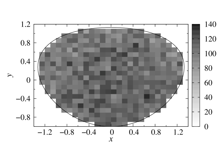
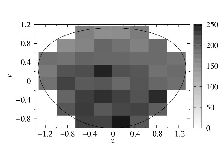
Figure 5: Dalitz-plot samples for $\eta^{\prime}\to\eta\pi^{+}\pi^{-}$ from the experimental Dalitz-plot distribution in Table 1 for the BES-III (top panel) and the VES (bottom panel) experiment.

In the following, we set up a scheme that allows us to fit both the experimental Dalitz-plot distribution and the partial decay width simultaneously and avoids some strong correlations between the fitting parameters.

First, we perform the following transformation of the fit parameters:

$$\alpha=\bar{\mathcal{N}}\bar{\alpha}\,,\quad\beta=\bar{\mathcal{N}}\bar{\beta}\,,\quad\gamma=\bar{\mathcal{N}}\bar{\gamma}\,.$$ (34)

Hence, we write the squared amplitude as

$$|\mathcal{M}(s,t,u)|^{2}=|\bar{\mathcal{N}}|^{2}|\bar{\mathcal{M}}(s,t,u)|^{2}\,,$$ (35)

where

$$\bar{\mathcal{M}}(s,t,u)=\bar{\alpha}\mathcal{M}_{\alpha}(s,t,u)+\bar{\beta}\mathcal{M}_{\beta}(s,t,u)+\bar{\gamma}\mathcal{M}_{\gamma}(s,t,u)\,,$$ (36)

and fix the arbitrary normalization of $\bar{\mathcal{M}}$ to

$$\int\text{d}x\,\text{d}y\,|\bar{\mathcal{M}}(x,y)|^{2}=1\,.$$ (37)

This condition results in a quadratic equation for the rescaled subtraction constants $\bar{\alpha}$, $\bar{\beta}$, and $\bar{\gamma}$. We choose to express $\bar{\gamma}$ in terms of $\bar{\alpha}$ and $\bar{\beta}$. The experimental partial decay width now directly determines the normalization $\bar{\mathcal{N}}$ and has no influence on the parameters $\bar{\alpha}$ and $\bar{\beta}$.

On the other hand, the experimental Dalitz-plot distribution (33) has again an arbitrary normalization. Hence, we have to fit the Dalitz-plot data according to

$$|\mathcal{M}_{\mathrm{exp}}|^{2}=|\mathcal{N}_{\mathrm{exp}}|^{2}\frac{|\bar{\mathcal{M}}|^{2}}{|\bar{\mathcal{M}}(x=y=0)|^{2}}=:|\mathcal{N}|^{2}|\bar{\mathcal{M}}|^{2}\,.$$ (38)

The Dalitz-plot distribution therefore determines the fitting parameters $\bar{\alpha}$, $\bar{\beta}$, and the irrelevant normalization $\mathcal{N}_{\mathrm{exp}}$ or $\mathcal{N}$.

Note that the experimental Dalitz-plot distribution is effectively described by three Dalitz-plot parameters $a$, $b$, and $d$. In the dispersive representation DR${}_{3}$, the shape of the Dalitz-plot distribution depends only on the two fitting parameters $\bar{\alpha}$ and $\bar{\beta}$. Therefore, the parametrization DR${}_{3}$ has predictive power. The representation DR${}_{4}$ describes the shape of the Dalitz-plot distribution again in terms of three parameters.

The result of the fit to data provides us with a representation of the amplitude that fulfills the strong constraints of analyticity and unitarity. This will be an essential input for a forthcoming dispersive analysis of $\eta^{\prime}\to 3\pi$ etaprimeto3pi.

The experimental partial decay width PDG

$$\Gamma (\eta^{\prime}\to\eta\pi^{+}\pi^{-})=\frac{1}{32(2\pi)^{3}\,M_{\eta^{\prime}}^{3}}\int\text{d}s\,\text{d}t|\mathcal{M}(s,t,u)|^{2}$$

$$=\frac{M_{\pi}Q_{\eta^{\prime}}^{2}}{128\pi^{3}\sqrt{3}M_{\eta^{\prime}}(M_{\eta}+2M_{\pi})}\int\text{d}x\,\text{d}y|\mathcal{M}(x,y)|^{2}$$

$$=(84.5\pm 4.1)\times 10^{-6}\,{\rm GeV}$$ (39)

fixes the normalization to

$$\bar{\mathcal{N}}=13.88\pm 0.34\,.$$ (40)

For the rescaled subtraction constants in the DR${}_{3}$ representation, the fit of the dispersive representation with central values of the phase input to the BES-III data sample Ablikim:2010kp leads to

$$\begin{array}{cc}& \begin{array}{ccc}& \overline{\alpha }& \overline{\beta }\\ \overline{\alpha }=-2.34\pm 0.26& 1.00& -1.00\\ \overline{\beta }=6.70\pm 0.83& & 1.00\end{array}\hfill \end{array}$$ (41)