The RedGOLD Cluster Detection Algorithm and its Cluster Candidate Catalogue for the CFHT-LS W1

Abstract

We present RedGOLD, a new optical/NIR galaxy cluster detection algorithm, and apply it to the CFHT-LS W1 field. RedGOLD searches for red-sequence galaxy overdensities while minimising contamination from dusty star-forming galaxies. It imposes an NFW profile and calculates cluster detection significance and richness. We optimise these latter two parameters using both simulations and X-ray detected cluster catalogues, and obtain a catalogue $\sim 80\%$ pure up to $z\sim 1$, and $\sim 100\%$ ($\sim 70\%$) complete at $z\leq 0.6$ ( $z\lesssim 1$) for galaxy clusters with $M\gtrsim 10^{14}\ {\rm M_{\odot}}$ at the CFHT-LS Wide depth. In the CFHT-LS W1, we detect 11 cluster candidates per $\rm deg^{2}$ out to $z\sim 1.1$. When we optimise both completeness and purity, RedGOLD obtains a cluster catalogue with higher completeness and purity than other public catalogues, obtained using CFHT-LS W1 observations, for $M\gtrsim 10^{14}\ {\rm M_{\odot}}$. We use X–ray detected cluster samples to extend the study of the X–ray temperature–optical richness relation to a lower mass threshold, and find a mass scatter at fixed richness of $\sigma_{lnM|\lambda}=0.39\pm 0.07$ and $\sigma_{lnM|\lambda}=0.30\pm 0.13$ for the Gozaliasl et al. (2014) and Mehrtens et al. (2012) samples. When considering similar mass ranges as previous work, we recover a smaller scatter in mass at fixed richness. We recover $93\%$ of the redMaPPer detections, and find that its richness estimates is on average $\sim 40-50\%$ larger than ours at $z>0.3$. RedGOLD recovers X-ray cluster spectroscopic redshifts at better than $5\%$ up to $z\sim 1$, and the centres within a few tens of arcseconds.

1 Introduction

Galaxy clusters are powerful probes of our cosmological models and the evolution of galaxies in dense environments. Galaxy clusters can be detected in different ways, tracing different cluster components. Using X–ray and submillimeter observations, it is possible to trace their gas, by its bremsstrahlung radiation (e.g., Voit, 2005), and through the Sunyaev-Zel’dovich effect (Sunyaev & Zeldovich, 1970). It is also possible to consider the stellar component of cluster galaxies and study their radiation in the optical or in the infrared. The analysis of multi-wavelength data permits us to detect clusters searching for early-type galaxy (ETG) overdensities, which dominate the inner regions of galaxy clusters, in agreement with the morphology-density relation (Dressler, 1980).

So far, many different methods have been developed to detect galaxy clusters using optical data: some works are based on the search of spatial overdensities through friends-of-friends algorithms (e.g., Wen et al., 2012), adaptive kernel techniques (e.g., Mazure et al., 2007; Adami et al., 2010) or Voronoi tessellations (e.g., Kim et al., 2002). Other methods are based on the detection of galaxies that lie on the red-sequence (Gladders & Yee, 2000; Thanjavur et al., 2009; Rykoff et al., 2014). In some cases, also the existence of a brightest central galaxy (Koester et al., 2007) is required. A widely used technique is the Matched filter cluster detection (Postman et al., 1996) that relies on detecting galaxies in one passband and searches galaxy clusters analysing the galaxy distribution, with the assumption of model profiles that fit the data (for example a characteristic galaxy cluster luminosity and a radial profile (e.g., Olsen et al., 2007; Grove et al., 2009). Milkeraitis et al. (2010) proposed a revised method, the so-called 3D-Matched-Filter, which uses a finding algorithm based on the luminosity and radial profile of galaxy clusters, and photometric redshifts.

The existence of several detection algorithms depends on the fact that the ideal method to detect galaxy clusters would produce a catalogue that includes all the real clusters (i.e. complete) and is not contaminated by false detections (i.e. pure). However, beside the noise and systematics in the observations, all detection techniques are affected by biases and selection effects, because of their basic assumptions on the nature or the morphology of galaxy clusters. As a consequence, the resulting cluster catalogue will reflect these assumptions, missing structures that do not fit the adopted cluster properties: for example, X–ray selected cluster catalogues are incomplete against gas–poor clusters, while optically detected cluster catalogues are contaminated by galaxy projections and may be incomplete against fossil groups, because of the fainter magnitudes of the companion galaxies with respect to the central one (Jones et al., 2003; Proctor et al., 2011).

This implies that the different detection techniques are complementary and, while the ideal method to detect all galaxy clusters does not exist, each method can be optimised for a certain class of clusters and groups.

In the next decade, large scale deep surveys in the optical and the near-infrared have been planned for understanding the nature of dark energy, such as the Large Synoptic Survey Telescope (LSST, LSST Dark Energy Science Collaboration, 2012), the European Space Agency’s Euclid mission (Laureijs et al., 2011), and the U.S. National Aeronautics and Space Administrations WFIRST Mission . These surveys will use galaxy clusters as cosmological probes, and, to do so, will need accurate estimates of the cluster mass. Their cluster samples will be detected by the analysis of multi-wavelength optical and infrared data, and cluster mass estimates will be derived from galaxy counts in these wavelengths (e.g., the optical richness). For this reason, there is a large effort in the cluster community to improve existing cluster detection algorithms in the optical and the near-infrared, and to optimise their performance.

In this paper we present RedGOLD, our cluster detection algorithm based on a revised red–sequence technique, and apply it to the CFHT-LS (Canada-France-Hawaii Telescope Legacy Survey; Gwyn, 2012) Wide 1 (W1) field. To validate and optimise our detection technique, we present a direct comparison with X–ray detected cluster catalogues and previous public catalogues based on different detection techniques in the optical.

The paper is organised as follows: in section 2 we describe the observations and the survey properties. We briefly present the photometric redshift estimates in section 3. In section 4 we present our detection technique and the optical richness provided by our algorithm. Section 5 is focused on the estimate of the completeness and the purity of our algorithm using both simulations and observations. In section 6 we discuss our results obtained applying the algorithm to the Canada-France-Hawaii Lensing Survey (hereafter referred to as CFHTLenS; Heymans et al., 2012) optical data and the comparison with existing publicly available cluster catalogues. Finally, in section 7 we present our conclusions.

We assume a standard cosmological model with $\Omega_{m}=0.3,\Omega_{\Lambda}=0.7$ and $H_{0}=70\ {\rm km\ s^{-1}\ Mpc^{-1}}$. If not differently specified, magnitudes are given in the AB system (Oke & Gunn, 1983; Sirianni et al., 2005).

2 Observations and data description

We apply our algorithm to the CFHT-LS W1 field, using the CFHTLenS reduction. Here we briefly summarise the CFHTLenS data that we use, and we refer the reader to Erben et al. (2013) for a detailed description of the survey properties. The CFHT-LS covers $154\ {\rm deg^{2}}$ in 5 optical bands, $u^{*},g,r,i,z$, observed with the MegaCam instrument (Boulade et al., 2003). The CFHTLenS survey analysis combined weak lensing data processing with THELI (Erben et al., 2013), shear measurement with lensfit (Miller et al., 2013), and photometric redshift measurement with PSF-matched photometry (Hildebrandt et al., 2012). A full systematic error analysis of the shear measurements in combination with the photometric redshifts is presented in Heymans et al. (2012), with additional error analyses of the photometric redshift measurements presented in Benjamin et al. (2013). The depth of the CFHT-LS deep and wide fields is $i\sim 27.4$ mag and $i\sim 25.7$ mag, respectively.

Among the four wide fields, we use images from the CFHT-LS W1 field, centred on the position RA=02:18:00 and DEC=-07:00:00, processed as described in Raichoor et al. (2014). Raichoor et al. (2014) used a modified version of the THELI pipeline (Erben et al., 2013) to reprocess the CFHT-LS W1 fields: they calibrated the zero points on the Sloan Digital Sky Survey (SDSS; York et al., 2000) and, for that reason, they analysed 62 out of the 72 pointings of the CFHT-LS W1, because the remaining 10 fields are not covered by the SDSS. They adopted the global PSF homogenisation method, described in Hildebrandt et al. (2012), because it significantly increases the accuracy of the colour measurements, and, as a consequence, the accuracy of the photometric redshifts. The final CFHT–LS W1 area that we use is then $\sim 60\ {\rm deg^{2}}$.

We calibrate our cluster detection algorithm using the X–ray catalogue provided by Gozaliasl et al. (2014). It covers 3 $\rm deg^{2}$ in the CFHT-LS W1 field and includes 135 X–ray groups and clusters up to redshift 1.1 with masses between $9.5\times 10^{12}<M_{200}<3.8\times 10^{14}\ M_{\odot}$. The median mass is $M_{200}=5.9\times 10^{13}\ M_{\odot}$.

We use both the Gozaliasl et al. (2014) catalogue and the XMM Cluster Survey (XCS) catalogue (Mehrtens et al., 2012) to study the X–ray temperature–optical richness relation. The XCS serendipitously searches for galaxy clusters, using the whole available data set in the XMM–Newton Science Archive. This catalogue includes 503 X–ray detected clusters up to $z\sim 1.5$, with 401 of them with an X–ray temperature measurement of $0.4<T_{X}<14.7$ keV. Of those, 27 detections are in the CFHT-LS W1 field, and we restrict our subsample to 20 objects with a temperature measurement of $0.6<T_{X}<7.5$ keV.

3 The photo-z catalogue

The photometric redshift estimates have been obtained as explained in Raichoor et al. (2014): they used the bayesian codes LePhare (Arnouts et al., 1999, 2002; Ilbert et al., 2006) and BPZ (Benítez, 2000; Benítez et al., 2004; Coe et al., 2006), and a set of 60 templates (Capak et al., 2004), obtained interpolating four empirical models (Ell, Sbc, Scd, Im; Coleman et al., 1980) and two starburst spectra (Kinney et al., 1996). For the LePhare photometric redshift estimates, they included the reddening as a free parameter ($0<E(B-V)<0.25$), considering the Small Magellanic Cloud (SMC) extinction law for late type galaxies (Prevot et al., 1984). They also introduced a new prior for the brightest objects.

To estimate the photometric redshift accuracy, Raichoor et al. (2014) used spectroscopic redshift measurements from different surveys: the VIMOS Public Extragalactic Redshift Survey (VIPERS; Guzzo et al., 2014), and the F02 and F22 fields of the VIMOS VLT Deep Survey (VVDS; Le Fèvre et al., 2005, 2013).

As shown in Raichoor et al. (2014), the photometric redshift quality decreases with increasing magnitude and with increasing redshift, with $\sigma_{photoz}\sim 0.03\times(1+z)$ at $i<23.5$ mag and a fraction of outliers of less than $9\%$. Similarly, the bias, defined as the median of $\Delta z=\frac{z_{\rm phot}-z_{\rm spec}}{1+z_{\rm spec}}$, is around zero for bright and low–redshift objects while it becomes larger for faint ($i>23.5$ mag) and high–redshift ($z>0.8$) sources.

4 The Cluster Detection Algorithm RedGOLD

Our algorithm, which we name RedGOLD (Red-sequence Galaxy Overdensity cLuster Detector), is based on the detection of red-sequence galaxy overdensities. It relies on the observational evidence that galaxy clusters host a large population of passive (red) and luminous (L>0.2 $\times L^{*}$) ETGs, mostly concentrated in their cores and tightly distributed on a red-sequence on the colour-magnitude diagram (Bower et al., 1992). This assumption is true for clusters of galaxies up to $z\sim 1.5$ (e.g., Mei et al., 2009; Snyder et al., 2012; Brodwin et al., 2013; Mei et al., 2015).

The method consists of two main steps, described in the following sections: (1) the detection of spatial overdensities of red early-type galaxies; (2) the confirmation of a tight red-sequence in the colour-magnitude relation.

4.1 Red galaxy overdensity detection

In order to detect spatial overdensities of red early–type galaxies, we eliminate all saturated objects and consider only galaxies with $i<23.5$ mag, to have uncertainties on photometric redshifts $\sigma_{photoz}\lesssim 0.03\times(1+z)$. This applies to all our procedure from now on, except to the cluster candidate richness estimate.

To identify stars, we remove objects with the SExtractor $CLASS\_STAR>0.95$ and $i<22.5$ mag, following Raichoor et al. (2014).

We divide the entire galaxy sample in redshift slices in the range $0.1<z<1.2$ with a step of $\delta z=0.2$ and overlapping by $3\times\sigma_{photoz}$. To take into account the errors on the galaxy photometric redshifts, we also select all galaxies with a photometric redshift within one $\sigma_{photoz}$ from a given redshift bin, where $\sigma_{photoz}$ is the error on the individual galaxy photometric redshift from Raichoor et al. (2014).

In each redshift bin, early-type galaxies have well defined red-sequence colours (i.e., colours of typical old stellar populations) which can be predicted with stellar population models (e.g., Mei et al., 2009).

We convert our observed magnitudes into absolute rest-frame magnitude, following Mei et al. (2009), using the corresponding galaxy photometric redshift and taking into account the filter corrections as in Mei et al. (2009). We adopt both a k-correction and an evolution correction as in Mei et al. (2009). To have the lowest possible contamination, we first select passive galaxies in two colours simultaneously. We choose two pairs of filters at each redshift bin, corresponding to the (U-B) and (B-V) rest-frame colours: doing so, the colour that corresponds to the (U-B) rest-frame colour straddles the 4000 Å break, and the joint colour cut, which corresponds to the (B-V) rest–frame, allows to separate red galaxies with ongoing or recent star-formation events from red passive galaxies (Larson & Tinsley, 1978).

To compute predicted colours in each redshift bin, we use single burst Bruzual & Charlot (2003) (BC03) stellar population models. We assume a passive evolution, a galaxy formation redshift $z_{form}=3$ and a solar metallicity, $Z=0.02$. In this work we adopt a Salpeter initial mass function (Salpeter, 1955).

In addition to our colour selection, we require that red galaxies are also defined as ETGs according to the classification provided by the Spectral Energy Distribution (SED) fitting used to estimate photometric redshifts, i.e. objects which show ETG spectral characteristics. In fact, in the redshift range that we consider, the galaxy morphological classification based on galaxy shapes and structural parameters is possible only for the brightest galaxies (and the lowest redshifts) with ground–based observations. Typically, the magnitude and redshift limits for ground–based observations morphological classification are $r<22$ mag and $z<0.5$ for ETGs (Pović et al., 2013).

To identify galaxy overdensities, in each MegaCam field, and for each redshift slice:

• We divide the coordinates space in overlapping circular cells of fixed comoving radius $r_{grid}=500$ kpc, and with centres separated by $500$ kpc;

• We count the number of red ETG galaxies $N_{gal}$ in each cell, and we build the galaxy count distribution in different redshift bins. We consider the background contribution $N_{bkg}$ as the mode of this distribution, and calculate its standard deviation $\sigma_{bkg}$, in each redshift bin;

• We estimate the detection significance $\sigma_{det}=\frac{N_{gal}-N_{bkg}}{\sigma_{bkg}}$ in each cell.

Since clusters are structures denser in red ETGs than the average red ETG background, we find our preliminary overdensity-based detections as systems characterised by red ETG densities larger than $N_{bkg}+\sigma_{det}\times\sigma_{bkg}$.

The choice of $\sigma_{det}$ changes the cluster catalogue completeness and purity (see section 5, in which we discuss our choice of $\sigma_{det}$). In Figure 1, we show an example of the galaxy count distribution for one CFHT-LS W1 MegaCam pointing at $z=0.5$: the red vertical line represents the detection limit $N_{bkg}+3\times\sigma_{bkg}$, implying that all structures lying on the right side of the chosen $N_{bkg}+\sigma_{det}\times\sigma_{bkg}$ are cluster candidate detections with $\sigma_{det}\geq 3$.

A preliminary cluster redshift is assigned as the central value of the redshift bin.

In the CFHTLenS data, for each science image, a mask flags regions with less accurate photometry (e.g. because of star haloes; Erben et al., 2013). Rykoff et al. (2014) pointed out that masks have to be taken into account not to underestimate the cluster richness and proposed a technique to extrapolate the richness measurement in regions with missing photometry (e.g. empty regions/holes).

In our case, we choose not to use an extrapolation technique. The way we take into account the presence of masks for the stars and other saturated objects is by selecting only objects with an error in photometry within the average distribution. In fact, the area over which the CFHTLenS catalogue is empty is very small ($\sim 10\%$) and the main difference in the photometry of galaxies in masked areas is the larger photometry uncertainties. We build a photometry uncertainty distribution in magnitude bins using Raichoor et al. (2014) photometry and photometric errors. We discard all objects that have uncertainties more than 3-$\sigma$ the average uncertainty distribution in the red overdensity calculation.

A posteriori, we verify that our procedure does not affect our detection efficiency and does not discard a significant number of real cluster members, leading to an underestimation of the cluster richness. We describe this procedure in more detail in section 5 and section 6.

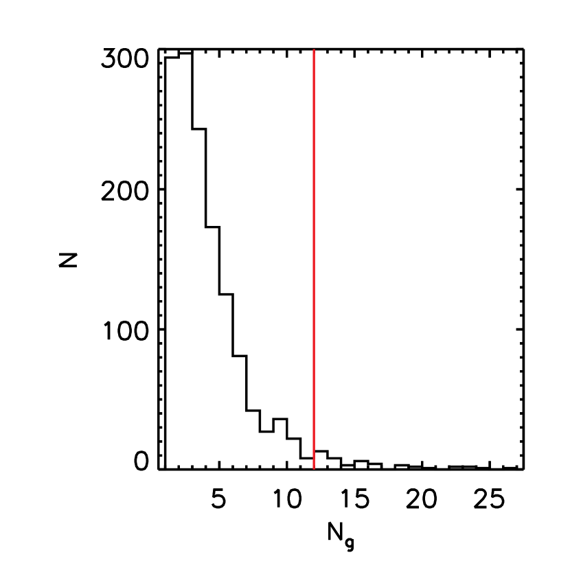
Figure 1: Example of our galaxy count distribution $N_{g}$. The red vertical line represents the $N_{bkg}+3\times\sigma_{bkg}$ limit at z=0.5 for one MegaCam pointing in the CFHT-LS W1.

4.1.1 Cluster centring

A key step of all detection algorithms is the cluster centring. The estimate of the centre is very important, as a miscentring can lead to an increasing in the scatter and in the slope of the colour-magnitude relation. The miscentring can also lead to a bias in the weak-lensing mass measurements (up to $\sim 30\%$; George et al., 2012), and in the cluster richness estimates (e.g., Johnston et al., 2007; Rozo et al., 2011).

The very simple idea underlying our centring technique is that, since red ETGs are mostly concentrated in the inner regions of galaxy clusters, we can centre our preliminary detections using local galaxy densities. Since George et al. (2011) has shown that centroids trace overdensity centres less efficiently than the brightest galaxies, we search for the brightest galaxy in the most overdense region. We consider all red ETGs brighter than $0.2\times{\rm L^{*}}$, and select as cluster centre the galaxy with the highest number of red ETG galaxies within a calibrated fraction of its cell, weighted on luminosity. For our application to the CFHT-LS W1, we calibrate the radius of this region with the available X–ray cluster centres from Gozaliasl et al. (2014), minimising the distance between our centres and the X–ray centres. If two or more galaxies correspond to the highest local density value, we simply centre our detection on the brightest one.

4.2 Colour-magnitude relation and red-sequence

To confirm our cluster candidates and refine our photometric redshift estimate, we analyse their colour-magnitude diagram.

Following Mei et al. (2009), we convert our observed colours at a given redshift into $(U-B)_{z=0}$ rest-frame colours using the relation :

$$(U-B)_{z=0}=Z_{point|(U-B)}+S_{(U-B)}\times col_{obs}\ ,$$ (1)

where $col_{obs}$ is the observed colour, and $Z_{point|(U-B)}$ and $S_{(U-B)}$ are the fit zero point and slope, respectively. We use BC03 single burst stellar population models, assuming a passive evolution, a formation redshift $1<z_{form}<7$ and three different values of metallicities (Z=0.008, 0.02 and 0.05). The rest-frame magnitudes are computed in the Vega system while observed magnitudes are in the AB system, following Mei et al. (2009).

We convert observed magnitudes in absolute B rest-frame magnitudes, $M_{B}$, by fitting the relation:

$$M_{B,z=0}=mag_{obs}+Z_{point|M_{B}}+S_{M_{B}}\times col_{obs}\ ,$$ (2)

where $mag_{obs}$ and $col_{obs}$ are the observed magnitude and colours for which we perform this conversion, and $Z_{point|M_{B}}$ and $S_{M_{B}}$ are the zero point and the slope of the linear fit, respectively.

In the age and metallicity range that we consider (consistent with the ETG old populations), there is a linear relation between the colours that straddle the 4000 Å break and the $(U-B)_{z=0}$ rest-frame colour (Mei et al., 2009). Errors on the relation zero point and scatter, due to the sampling that we are using, are estimated through jackknife. Errors on the relation zero point and scatter, due to the sampling that we are using, are estimated through jackknife applied to galaxies.

The observed magnitudes are chosen to be the closest to the rest-frame U and B magnitudes.

From the estimated $(U-B)$ and $M_{B}$, we perform a robust linear fit on the $(U-B)$ vs $M_{B}$ relation, using the Tukey’s biweight (Press et al., 1992). Mei et al. (2009) did not find a significant evolution in the colour-magnitude parameters as a function of redshift (confirmed by Snyder et al., 2012): the average slope and intrinsic scatter for early-type galaxies (E+S0) are $\frac{\Delta{(U-B)_{z=0}}}{\Delta_{M_{B,z=0}}}=-0.046\pm 0.023$ and $\sigma_{(U-B)_{z=0}}=0.061\pm 0.015$ mag, respectively. For this reason, we impose that our detections have a red-sequence scatter and slope within $3\sigma$ of the expected value estimated from Mei et al. (2009) (mean value of the red-sequence parameters plus three times the scatter, adding in quadrature the photometric errors).

To refine the cluster candidate redshift, we use the ETG median photometric redshift. For each cluster candidate, we assign cluster membership to galaxies corresponding to the spatial overdensity if the difference between the galaxy photometric redshift and the cluster candidate redshift is within 3 times the uncertainty on photometric redshifts, $\sigma_{photoz}$. In our samples, the uncertainty on photometric redshifts is larger than the intrinsic redshift dispersion due to the cluster galaxy dispersion velocities.

4.3 Multiple detections

A very common problem for every cluster detection algorithm is that of multiple detections, i.e. the fact that the same structure is detected multiple times (e.g., in different redshift bins or different spatial regions).

Since we centre our preliminary detections on the red ETG with the highest local density, two preliminary detections that are spatially close can converge in similar centre positions.

For this reason, we develop an algorithm to clean the final cluster catalogue, in order to minimise the contamination due to multiple detections: in particular, we iteratively filter our catalogue, checking for detections characterised by at least half of members in common and with a final cluster candidate redshift difference of $\Delta z\leq 0.1$.

When a multiple detection is found, we retain as its centre the centre of the greatest red overdensity, characterised by the highest signal-to-noise ratio i.e. $\sigma_{det}$, weighted on luminosity. Applying these corrections, we are able to remove overlapping detections.

4.4 Optical richness

The estimate of the cluster richness is a key point when studying galaxy clusters, because the cluster richness is a proxy for the cluster mass, which is not directly measurable.

Several mass proxies have been adopted in the literature. For example, the X–ray luminosity $L_{X}$ is commonly adopted as a mass $M$ proxy. Vikhlinin et al. (2009) found that the scatter in mass at fixed $L_{X}$ is $\sigma_{lnM|L_{X}}\sim 0.25$ and Mantz et al. (2010) $\sigma_{lnM|L_{X}}\sim 0.32$. When using weak–lensing analysis to obtain cluster mass measurements, the scatter in the halo mass at fixed weak–lensing mass is of the same order of magnitude, $\sigma_{lnM|WL}\sim 0.3$ (Becker & Kravtsov, 2011; von der Linden et al., 2014). Similarly, a key measurement of optical detected clusters is the cluster richness, adopted as cluster mass proxy. For the MaxBCG catalogue (Koester et al., 2007), using X–ray and weak lensing mass estimates, Rozo et al. (2009a) found a relatively high scatter for the mass–richness relation at fixed richness $N_{200}$, $\sigma_{lnM|N_{200}}\sim 0.45$. Later, Rozo et al. (2009b) adopted an optimised cluster richness estimator $\lambda$, estimated considering the radial cluster density profile, the cluster luminosity function and the cluster galaxy colour distribution. When assuming the optimised $\lambda$ richness estimator, Rozo et al. (2009b) found $\sigma_{lnL_{X}|\lambda}=0.69$, representing a significant improvement with respect to the X–luminosity–$N_{200}$ relation, $\sigma_{lnL_{X}|N_{200}}=0.86$. Rykoff et al. (2012) analysed different possible sources of increased scatter in the mass–richness relation and optimised the $\lambda$ estimator, finding a smaller value for the scatter $\sigma_{lnL_{X}|\lambda}\sim 0.63$, which corresponds to a scatter in mass at fixed richness $\sigma_{lnM|\lambda}\sim 0.3$.

With the goal of minimising the scatter in the mass–richness relation and to find the best optical mass proxy, several optical richness definitions have been adopted in the literature. These definitions can be divided in two main groups. For the first group, the richness estimate is based on galaxy counts within a given magnitude range in a given spatial region (e.g. Koester et al., 2007; Andreon & Hurn, 2010). For the second group, the richness is measured from the galaxy spatial distribution, assuming cluster profile models as the Navarro–Frenk–White (NFW; Navarro et al., 1996) and the galaxy luminosity function, such as the Schechter (Schechter, 1976) luminosity function (e.g., Postman et al., 1996; High et al., 2010; Rozo et al., 2009b; Ascaso et al., 2012; Rykoff et al., 2014).

We define our richness estimate in the following way:

• We count for each redshift bin, the number of red ETGs (as defined above) in a given scaling radius $R_{scale}$ and brighter than $0.2\times{\rm L^{*}}$;

• We set an initial cluster candidate comoving size $R_{scale}=1.0\ {\rm Mpc}$ and we estimate the corresponding richness;

• We iteratively scale $R_{scale}$ according to the relation $R_{scale}=(\lambda/100)^{\beta}$, with $\beta=0.2$, until the difference in richness for two successive iterations is less than $N_{bkg}$.

Following Rykoff et al. (2014), we adopt $\beta=0.2$. A posteriori, we test different values of $\beta$ and we find that $\beta=0.2$ minimise the number of RedGOLD detections without an X–ray counterpart in the Gozaliasl’s catalogue. Typical values of $R_{scale}$ are between 0.5 and 1.0 Mpc.

At each iteration, we subtract the background contribution that corresponds to the same area and to the redshift bin in which the galaxy counts are computed.

4.5 Concentration parameter

Galaxy clusters are characterised by similar radial profiles and the galaxy density in the cluster centre can be an order of magnitude (or more) higher than that in the peripheral regions (e.g. following the dark matter NFW profile). To take this into account, we impose an additional constraint on the radial distribution of the red–sequence galaxies (see also Rykoff et al., 2014). Doing this, we are assuming that red galaxies follow the same profile distribution as dark matter. Our assumption is justified both theoretically by the fact that galaxies are collissionless as dark matter, and observationally (Lin et al., 2004; Collister & Lahav, 2005; Holland et al., 2015). Because of the singularity of the NFW profile at $R=0$, we adopt a core radius $r_{core}=0.1\ h^{-1}$ Mpc and we assume that the surface density profile is constant for $r\lesssim r_{core}$, following Rykoff et al. (2012).

We estimate a typical cluster NFW surface density profile $\Sigma(r)$ following Bartelmann (1996), in four radii corresponding to $R_{025}=0.25\times{R_{200}},\ R_{050}=0.5\times{R_{200}},\ R_{075}=0.75\times{R_{200}}$, and $R_{1}=1\times{R_{200}},$ and we compare the ratios of the observed surface density profile estimated at different radii with the value predicted by the NFW profile.

We adopt the mass–redshift–concentration relation from Duffy et al. (2008):

$$c=A\left(\frac{M}{M_{piv}}\right)^{B}(1+z)^{C}$$ (3)

with $M_{piv}=2\times 10^{12}\ {\rm h^{-1}M_{\odot}}$. Duffy et al. (2008) estimated the best–fit parameters A, B and C for relaxed systems ($A=6.71\pm 0.12$, $B=-0.091\pm 0.009$, $C=-0.44\pm 0.05$), and for the full cluster sample ($A=5.71\pm 0.12$, $B=-0.084\pm 0.006$, $C=-0.47\pm 0.04$), for the dark matter halo mass range $10^{11}-10^{15}\ {\rm M_{\odot}}$ and the redshift range $0<z<2$. These values are in agreement with recent work in the literature (e.g. Dutton & Macciò, 2014; Klypin et al., 2014).

We identify cluster candidates allowing the full cluster sample concentration to vary within $3\sigma_{c}$, with $\sigma_{c}$ being the uncertainty on the concentration $c$ from propagation of the uncertainties on $A$, $B$, and $C$ given above. In particular, we compare the ratios between the observed surface density profile at the four different radii ($\Sigma(R_{025})/\Sigma(R_{050})$, $\Sigma(R_{050})/\Sigma(R_{075})$ and $\Sigma(R_{075})/\Sigma(R_{1})$) with the theoretical values obtained above, and retain only the RedGOLD detections with observed profiles consistent with the NFW profile for all four radii, in the NWF profile range within $3\sigma_{c}$.

None of our cluster candidates are over–concentrated, i.e. show a concentration larger than $c+3\sigma_{c}$. Imposing our limit on the galaxy radial profile, we discard  6% of our candidates, all with a shallower (with respect to Duffy et al. (2008)) galaxy distribution. We visually check these excluded detections and we find that they are poorer and smaller systems.

5 Completeness and purity of our algorithm

5.1 Completeness versus Purity

In the literature, there are different methods to detect galaxy clusters. However, any technique suffers for some incompleteness and contamination effects: for each algorithm, it is necessary to find a good compromise between completeness and purity. The Completeness is defined as the ratio of detected structures which correspond to a true cluster $N^{det}_{true}$ to the total number of true clusters $N_{true}$:

$$Completeness=\frac{N^{det}_{true}}{N_{true}}\ .$$ (4)

The Purity is the total number of detection $N_{det}$ minus the fraction of false detections $N_{false}$ to the number of detected objects.

$$Purity=\frac{N_{det}-N_{false}}{N_{det}}$$ (5)

The completeness quantifies how well a detection algorithm is able to find true clusters (i.e. the probability that a detection algorithm will detect true clusters), while the purity estimates the percentage of true clusters (as opposite to false detections) detected by the algorithm (i.e. the probability that a detection corresponds to a true cluster). These are two key quantities to determine the goodness of any cluster catalogue and the ideal algorithm is characterised by simultaneously high values of completeness and purity.

In practice, it is very difficult to maximise both quantities at the same time and it is common to find instead a good compromise. To find the best compromise between completeness and purity, we first test RedGOLD on semi-analytic simulations and then on already known X–ray detected clusters.

In both definitions of completeness and purity, it is important to define a true and a false cluster. Following the literature (e.g, Finoguenov et al., 2003; Lin et al., 2004; Evrard et al., 2008; Finoguenov et al., 2009; McGee et al., 2009; Mead et al., 2010; George et al., 2011; Chiang et al., 2013; Gillis et al., 2013; Shankar et al., 2013), we define a true cluster as a dark matter halo more massive than $10^{14}\ \rm M_{\odot}$, since numerical simulations show that 90$\%$ of the dark matter haloes more massive than $10^{14}\ M_{\odot}$ are a very regular virialised cluster population up to redshift $z\sim 1.5$ (e.g., Evrard et al., 2008; Chiang et al., 2013). We define true galaxy groups, dark matter haloes with mass $10^{13}\ M_{\odot}<M<10^{14}\ M_{\odot}$. Within our definitions, dark matter haloes with lower masses are not considered as a group or cluster detection, but as field galaxies.

Since we want to optimise RedGOLD to detect galaxy clusters, we estimate its completeness with respect to dark matter haloes more massive than $10^{14}\ \rm M_{\odot}$. However, because of the scatter $\sigma_{mass}$ in the scaling relations between cluster dark matter halo mass and measured mass proxies (Rozo & Rykoff, 2014; Rozo et al., 2014), we cannot consider as false detections the cluster candidates with mass within $\sim 3\times\ \sigma_{mass}$ from a typical scaling relation. As discussed in section 4.4 the typical scatter in the observed mass scaling relations is $\sigma_{lnM|M_{proxy}}\sim 0.3$, where $M$ is the mass estimate for the dark matter halo, and $M_{proxy}$ is the used mass proxy (e.g. $L_{X}$, $N_{200}$, $\lambda$, etc). For this reason, we estimate the purity of our algorithm with respect to dark matter haloes more massive than $10^{13}\ M_{\odot}$. We have also tested a lower limit in mass, and when estimating the purity with respect to dark matter haloes more massive than $10^{12.5}\ \rm M_{\odot}$, its estimated value changes by only $9\times 10^{-4}$.

5.2 Completeness and purity of our algorithm from Millennium Simulation

We apply our detection algorithm to the Millennium Simulation (Springel et al., 2005): among the different realisations of mock galaxy catalogues based on semi-analytic models, we use the lightcones by Henriques et al. (2012), which consist of 24 independent beams, and have been built from the model by Guo et al. (2011). In fact, the Guo et al. (2011) semi-analytic model matches the local SDSS luminosity and stellar mass function, obtaining a good agreement with the observations. Before using them to test RedGOLD, we have taken into consideration some properties of the model that can introduce systematics in our detection procedure. In fact, although many improvements have been made with respect to previous simulations (e.g. the stellar mass function), the Guo model still shows some discrepancies with the observations: in particular, galaxy colours are difficult to reproduce in an accurate way, since they depend on different parameters, as metallicity, star-formation history and dust.

Guo et al. (2011) showed that at z=0 there is a discrepancy between the colours predicted in their models and the SDSS observations, over-predicting the fraction of red dwarf galaxies ($M<10^{9.5}\ {\rm M_{\odot}}$), with colours redder than observed. On the other hand, at $M>10^{10.5}\ {\rm M_{\odot}}$, the colours are bluer with respect to the observations.

Since Guo et al. (2011) simulated ETG spectral energy distributions for galaxies with $B/T\geq 0.7$ (see also Shankar et al. (2014)), we select galaxies with $B/T\geq 0.7$ as ETGs. We find that the ETG abundance in galaxy clusters is not well reproduced, and the ETG fraction is systematically underestimated. Clearly, this deeply affects the results obtained with our algorithm, since it relies on the search of red–sequence ETGs.

This discrepancy affecting semi-analytic models has been already noted in previous works: for example, Cohn et al. (2007) compared the red-sequence of simulated galaxies in the Millennium Simulation (Springel et al., 2005; Croton et al., 2006; Kitzbichler & White, 2007) with the observations, finding that the simulated red-sequence has a larger scatter and a positive slope while the observed slope is negative. Also Hilbert & White (2010) investigated the effect of this discrepancy between models and observations, finding that it is crucial to correct for it when using optical cluster finding algorithms with simulations. In particular, they measured the mean colour of red–sequence galaxies for mock galaxies as a function of redshift and they compared it with the same relation obtained from SDSS galaxies, finding that the mean red–sequence galaxy colour obtained from semi-analytic models is quite close to the SDSS ones at very low redshift, but the discrepancy between the two become significant at higher redshifts. They explicitly noted that, without any adjustment in colours, they would have not found almost any clusters at $z>0.25$.

As our detection technique relies on the search of the red–sequence ETGs, we have to take into account these effects. As a consequence, to have a reliable estimate of completeness and purity, we correct the mock catalogues in order to obtain a realistic galaxy type distribution in simulated clusters, and accurate colours.

For the lightcones by Henriques et al. (2012), up to the galaxy luminosities that we are considering in this work, we find that:

• all clusters have a negligible fraction of bulge-dominated red galaxies; $\sim 70\%$ of haloes more massive than $10^{14}\ {\rm M_{\odot}}$ and at $z\leq 1.1$ have less than 5 bulge-dominated members with colours matching the BC03 predictions for passive galaxies (see also Ascaso et al., 2015); on the other hand, observed clusters up to $z\sim 1.5$ show ETG fractions of $70-80\%$ (e.g., Postman et al., 2005; Desai et al., 2007; Mei et al., 2009, 2012; Brodwin et al., 2013);

• $\sim 10\%$ of the simulated clusters show positive slope (while observations show negative slopes) and/or wider scatter of red-sequence galaxies with respect to observations;

• at a given redshift, on the red-sequence there is a shift between simulated ETG colours from the semi-analytic model and ETG colours predicted from the BC03 stellar population models, with the lightcone colours being bluer.

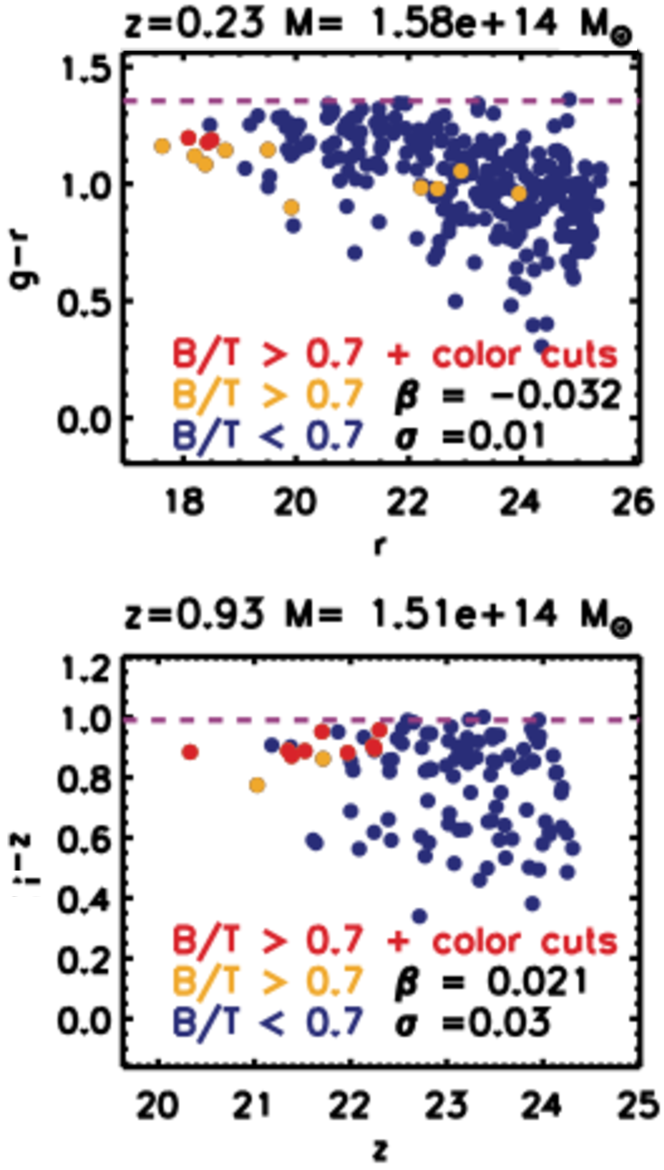
Figure 2: Original colour-magnitude relation of two clusters in the Henriques et al. (2012) lightcones at $z=0.23$ (top panel) and $z=0.93$ (bottom panel). Blue circles are cluster members, orange symbols represent members with $B/T\geq 0.7$ (i.e. ETGs) and red circles are ETGs characterised by colours in agreement with predictions from BC03 models for passive galaxies at the same redshift. The purple dashed line shows the mean colour predicted by the BC03 models. The $\sigma$ and $\beta$ values refer to the red–sequence scatter and slope.

Figure 2 shows two examples of the colour-magnitude relation for two massive clusters in the lightcone catalogues, at redshift $z=0.23$ and $z=0.93$: blue circles are cluster members, orange circles represent ETGs, i.e. members with $B/T\geq 0.7$, and red circles are ETGs with colours in agreement with those predicted by BC03 models for passive galaxies at the same redshifts. The purple dashed line shows the ETG colour predictions by single burst BC03 models, assuming passive evolution, $z_{form}=3$ and solar metallicity. Both problems are clearly visible: the total number of ETGs is negligible and only a small fraction of ETGs matches the BC03 predicted colours, leading, in one of these two cases, to a positive red-sequence slope.

These results imply that we have to correct for both the colour mismatch of red ETGs and the low fraction of early–type galaxies. In the following section, we will describe how we implement these corrections and give a final estimate for purity and completeness.

5.2.1 Mock catalogue corrections

The first modification that we need to apply to run RedGOLD on the Henriques et al. (2012) lightcones is to obtain red-sequence colours from the simulations to identify red overdensities (instead of using predictions from the BC03 models, that are inconsistent with the red-sequence in the simulations).

Since we should modify colours for both early and late type galaxies in all environments, we do not change the colours in the mock catalogues to avoid to introduce biases in the galaxy properties and their large-scale distribution. For this reason, instead of changing the colours in the lightcones, we estimate the expected red-sequence ETG colours used by RedGOLD to match the Henriques et al. (2012) red-sequence colours.

We consider all ETGs (objects with $B/T\geq 0.7$) brighter than $0.2\times{\rm L^{*}}$ from the lightcone cluster catalogues, in narrow redshift slices of 0.05, and we build the histogram of galaxy colours for each redshift bin. In each redshift bin, we fit this distribution with a Gaussian and we obtain its mean $\bar{c}$ and its standard deviation $\sigma_{col}$ as a function of redshift. These are the expected red-sequence ETG colour and its intrinsic scatter, which we use for our RedGOLD red overdensity detections.

The second discrepancy in the Henriques et al. (2012) simulation is the low fraction of ETGs on cluster red-sequences (i.e. galaxies with $B/T\geq 0.7$): in fact, since RedGOLD detects red early-type galaxy overdensities, it is necessary that the clusters in the simulation have realistic ETG fractions.

Although Guo models are able to reproduce the galaxy distribution for different morphological types in the local Universe (see Figure 4 in Guo et al., 2011), there is a lack of early-type galaxies in clusters at $z\apprge 0.1$. In observed clusters, groups and the field up to $z\sim 1.5$, the ETG fraction is of $\sim 70\%\pm 10\%$, $\sim 50\%\pm 10\%$, and $\sim 30\%\pm 10\%$, respectively, up to the magnitude limits considered in this work (e.g., Treu et al., 2003; Desai et al., 2007; Postman et al., 2005; Smith et al., 2005; Mei et al., 2009; George et al., 2011; Mei et al., 2012). To correct for this discrepancy, we modify Guo et al. (2011) galaxy morphologies in the cluster, group and field red-sequence, to reproduce these observed fractions. Since our detection code searches for red ETG overdensities, if we modify the ETG fractions only in clusters, we would obtain optimistic values for the completeness and purity, as groups and field ETGs are not enhanced. For this reason, to have a coherent scenario, we also modify the ETG fraction in groups and in the field.

We distribute the cluster, group and field ETGs around the mean red-sequence colour, following a Gaussian distribution with standard deviation equal to the intrinsic red-sequence scatters that we have derived above for the lightcones (i.e. $68\%$ of the ETGs will be distributed in 1 $\sigma_{col}$). Since we modify the percentages in the same way at all luminosities, we do not expect to change in a significant way the shape of the ETG luminosity function in the luminosity range considered for the cluster detection with RedGOLD.

In Figure 3, we show the corrected colour-magnitude-relation for the two clusters shown in Fig. 2, after applying this procedure. For the RedGOLD detection procedure, we use the average red-sequence colours at each redshift from Henriques et al. (2012) colours, and modify ETG fractions to be consistent with the observations. When these corrections are applied, we find that only $\sim 5\%$ of clusters have less than 5 ETGs or wrong values for the red-sequence scatter and/or slope, and in all cases they are massive structures lying on the edges of the lightcones. When applying these corrections, the red–sequence is well reproduced: both the red–sequence scatter $\sigma$ and slope $\beta$ are in agreement with the observations.

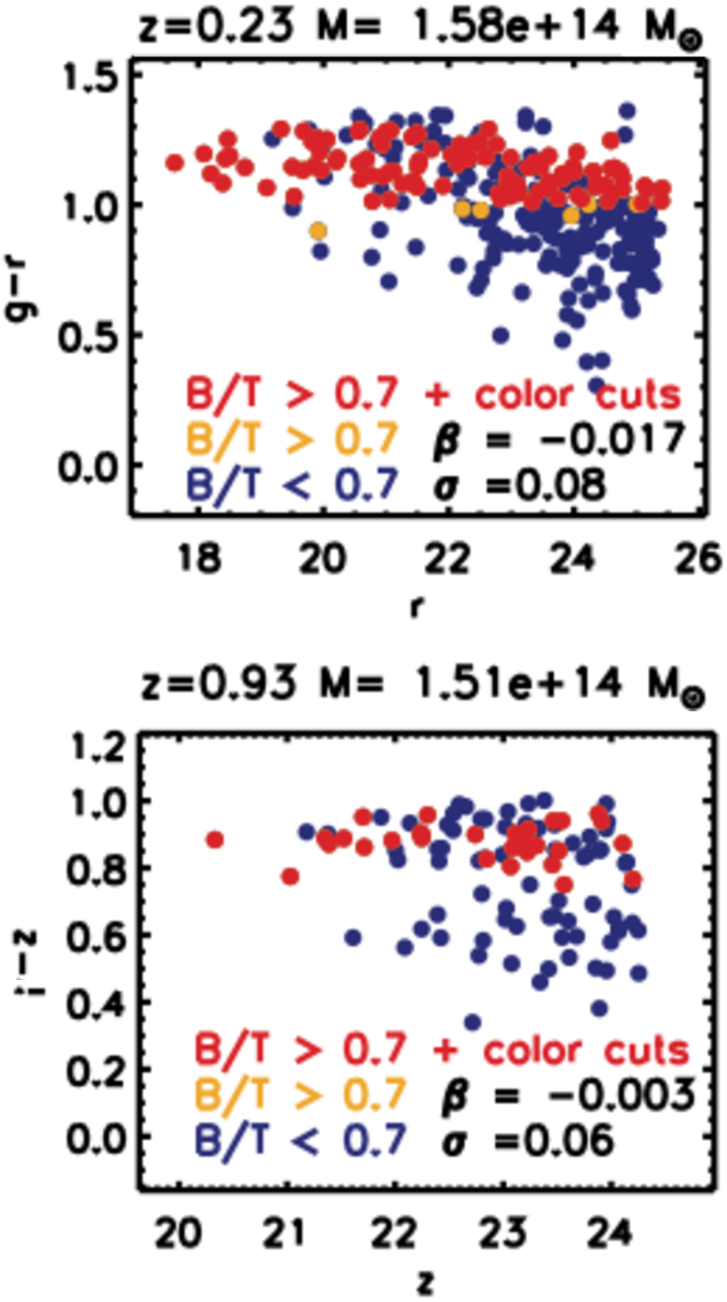
Figure 3: Modified colour-magnitude relation of the two clusters in the Henriques et al. (2012) lightcones at $z=0.23$ (top panel) and $z=0.93$ (bottom panel) shown in Fig. 2 after our correction procedure. Symbols are the same as Fig. 2. Within RedGOLD, we use the average red-sequence colours at each redshift from the Henriques et al. (2012), and modify the ETG fractions to be consistent with the observations. The $\sigma$ and $\beta$ values refer to the red–sequence scatter and slope.

5.2.2 Magnitude and colour uncertainties

Since we want to have galaxy simulations with a photometric accuracy that is representative of the CFHTLenS data, we modify simulated galaxy magnitudes from the Henriques et al. (2012) lightcones, to reproduce the CFHTLenS photometric errors.

We convert the SDSS magnitudes in the Henriques et al. (2012) catalogues in CFHT/MegaCam magnitudes, $u^{*},g,r,i,z$, following Ferrarese et al. (2012). For each bandpass, we then compute the mean photometric error $\bar{\epsilon}$ and the corresponding uncertainty $\sigma_{\epsilon}$ (in magnitude bins of 0.1 mag) in the CFHTLenS data, and we use them to correct magnitudes and errors in Henriques et al. (2012) catalogues. We add the mean error to each simulated magnitude, following a Gaussian distribution, and randomly assign magnitude uncertainties as a function of magnitude.

For the same reason, we modify the redshifts in the lightcones to reproduce the same accuracy of the CFHTLenS redshift estimates: in particular, we change the photometric redshifts randomly extracting values from a Gaussian centred on the true redshift value and with a standard deviation $\sigma_{photoz}$, following the values reported in Raichoor et al. (2014) as a function of magnitude. Following the same procedure used to add uncertainties to magnitudes, we add uncertainties in photometric redshifts. To reproduce the outlier fraction as observed in the CFHTLenS, we assign to a percentage of objects, that corresponds to the observed percentage of outliers, a random photometric redshift, which differs from the original of $\Delta z>0.15$ (according to the definition of outliers).

5.2.3 CFHTLenS masked regions

To test the effect of the masks on our detections, we build a second series of simulation to take into account the CFHTLenS masked regions from Erben et al. (2013), which include both masked regions without any source detections (e.g. empty regions/holes), and masked regions with higher photometry uncertainties. Firstly, we build an empirical size distribution of the holes and of the regions with photometric uncertainties higher than the average (i.e. the observed masked regions) from the CFHTLenS. Then, we add to our modified Millennium Simulations random masked circular regions extracted from this distribution. We assign to the galaxies in the regions with photometric uncertainties higher than the average, a random distribution of uncertainties derived from the one observed in the CFHTLenS corresponding masked regions. To do so, we build an uncertainty distribution for each magnitude bin, and calculate its mean and standard deviation.

We call these simulations, the masked modified Millennium. We run RedGOLD on both the modified Millennium Simulation (i.e. without masks) and the masked modified Millennium. As explained in section 4.1, in both cases we select only objects with an error in photometry within the average distribution.

5.2.4 Results

Our main goal is to test RedGOLD as red ETG overdensity cluster detector (steps described in the first three subsections of section 4), applying it to the simulations. We run RedGOLD on the modified Henriques et al. (2012) galaxy catalogues, and obtain a cluster candidate catalogue. For each detection, we obtain position, redshift and detection significance, and estimate purity and completeness as a function of significance, redshift, and halo mass.

We do not impose a cluster profile and do not estimate richness in this simple test. In fact, since the mock catalogues show a lack of bright red–sequence galaxies, richness measurements are biased towards lower values, and are not correlated with dark matter halo mass in the same way as in the observations. Moreover, since we use the scaling radius $R_{scale}$ (estimated from the cluster richness) to derive $R_{200}$, we cannot impose any limit on the cluster profile. As a consequence, the results obtained using the Millennium Simulations might represent a pessimistic scenario.

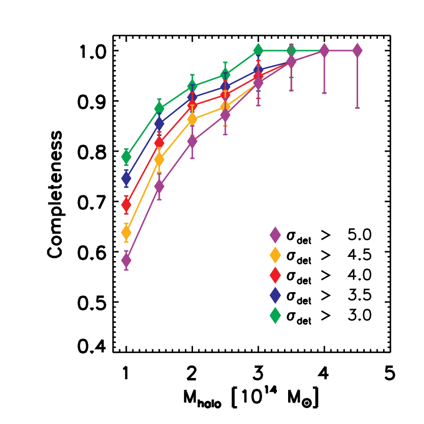
Figure 4: Completeness as a function of the halo mass in the entire redshift range $0<z<1.1$ obtained using the lightcones by Henriques et al. (2012). Green, blue, red, orange and purple symbols refer to $\sigma_{det}\geq 3,3.5,4,4.5,5$, respectively. Our completeness is always $>80\%$ for the most massive clusters ($M>2.5\times 10^{14}\ {\rm M_{\odot}}$), and does not change significantly for different values of $\sigma_{det}$. In the mass range $10^{14}<M<2.5\times 10^{14}\ {\rm M_{\odot}}$, the completeness changes significantly when considering different detection significance thresholds.

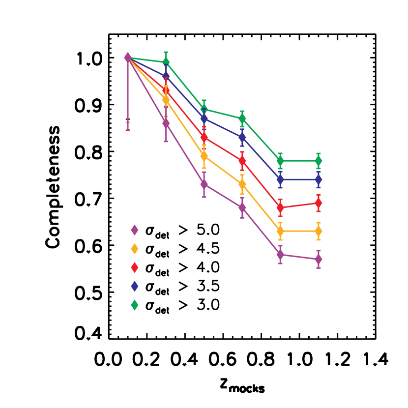
Figure 5: Completeness as a function of the redshift for haloes more massive than $10^{14}\ M_{\odot}$, obtained using the lightcones by Henriques et al. (2012). Symbols are as in Fig. 4. At low redshift ($z\lesssim 0.4$) RedGOLD is always $>80\%$ complete for all the considered $\sigma_{det}$ values. At higher redshift, though, increasing the detection significance corresponds to higher difference in the completeness as a function of $\sigma_{det}$.

To match the RedGOLD cluster candidates with the simulated dark matter haloes, we adopt a maximum projected distance between the centres corresponding to $R_{200}$ and $\Delta z=|z_{sim}-z_{RedGOLD}|\leq 3\times\sigma_{photoz}=3\times 0.03\times(1+z)$, where $z_{sim}$ is the cluster redshift in the simulations and $z_{RedGOLD}$ is the cluster redshift estimated by our algorithm.

In Fig. 4 and Fig. 5, we show the cluster completeness as a function of the dark matter halo mass in the entire redshift range $0<z<1.1$ and as a function of the redshift for haloes more massive than $10^{14}\ M_{\odot}$, respectively, for different values of the detection significance, $\sigma_{det}$. Green, blue, red, orange and purple symbols refer to $\sigma_{det}\geq 3,3.5,4,4.5,5$, respectively.

The error bars represent the uncertainties estimated following Gehrels (1986). These approximations provide the lower and upper limit of a binomial distribution within the $84\%$ confidence limit (i.e. $1\sigma$) and hold even when the completeness and the purity are estimated from small numbers (e.g. at high mass or low redshift). Using this conservative approach, our uncertainties are slightly overestimated (Cameron, 2011).

We define as clusters all dark matter haloes with mass $M_{halo}\geq 10^{14}\ {\rm M_{\odot}}$ (see section 5).

When we consider the entire redshift range $0<z<1.1$, our completeness is always $>80\%$ for the most massive clusters ($M_{halo}>2.5\times 10^{14}\ {\rm M_{\odot}}$), and does not change significantly for different values of $\sigma_{det}$. On the other hand, in the mass range $10^{14}<M_{halo}<2.5\times 10^{14}\ {\rm M_{\odot}}$, the completeness changes significantly when considering different detection significance thresholds: at $\sigma_{det}\geq 5$, RedGOLD misses $\sim 40\%$ of the less massive clusters ($M_{halo}\sim 10^{14}\ {\rm M_{\odot}}$). When we consider all masses ($M_{halo}>10^{14}\ {\rm M_{\odot}}$), at low redshift ($z\lesssim 0.4$) RedGOLD is always $>80\%$ complete from $\sigma_{det}\geq 3$ to $\sigma_{det}\geq 5$. At higher redshift, though, increasing the detection significance corresponds to larger differences in the completeness as a function of $\sigma_{det}$ (Fig. 5).

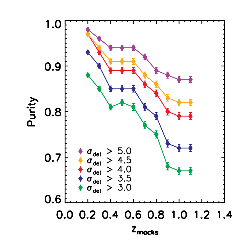
Figure 6: Purity as a function of the redshift, obtained using the lightcones by Henriques et al. (2012). Symbols are as in Fig. 4. The purity is $\gtrsim 80\%$ up to redshift $z\sim 1.2$ and $\sigma_{det}>4$.

In Fig. 6, we plot the purity as a function of the redshift. To estimate the purity, we consider all detected haloes with more than five members and more massive than $M_{halo}=10^{13}\ {\rm M_{\odot}}$ (see section 5.1). Similar choices have been adopted in previous work (Milkeraitis et al., 2010; Soares-Santos et al., 2011).

As in Fig. 5, we show our results as a function of the redshift and the detection significance. The purity as a function of redshift reaches higher values for higher $\sigma_{det}$ thresholds, as expected. For $\sigma_{det}\geq 5$, RedGOLD is pure at $>90\%$ at all redshifts, but, as shown in Fig. 4 and 5, the completeness is significantly lower than for other thresholds. In all cases, the purity is $\gtrsim 80\%$ up to redshift $z\sim 1.2$ and $\sigma_{det}>4$. This means that even if we reach a relatively low completeness ($\sim 65\%$) in detecting clusters at $1<z<1.2$, we can still obtain a very high purity at this significance.

At $\sigma_{det}\geq 4,4.5$ the purity is comparable with that reached considering $\sigma_{det}\geq 5$, being $>80-85\%$ in the whole redshift range. At $\sigma_{det}\geq 3,3.5$, the purity starts to be significantly lower, especially at $z\gtrsim 0.6$. To keep a purity $>80\%$ up to $z\sim 1$, our results show that we require a $\sigma_{det}\geq 4$.

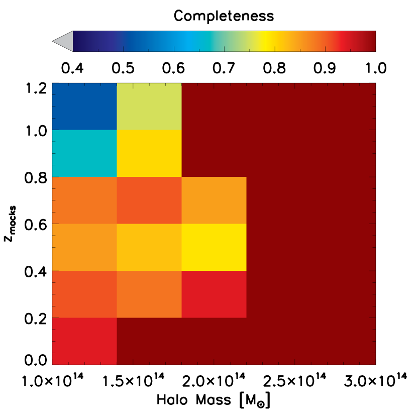
Figure 7: Completeness as a function of the halo mass and the redshift, obtained using the lightcones by Henriques et al. (2012), and assuming $\sigma_{det}\geq 4$. The completeness is $>80\%$ for $M_{halo}\gtrsim 2\times 10^{14}\ {\rm M_{\odot}}$ and $z<1.1$. For $10^{14}\ {\rm M_{\odot}}<M_{halo}\lesssim 2\times 10^{14}\ {\rm M_{\odot}}$, it decreases at $65-70\%$ at $z>0.8$, and significantly depends on the halo mass.

Fig. 7 shows the completeness as a function of the halo mass and the redshift, assuming $\sigma_{det}\geq 4$. RedGOLD always reaches a completeness $>80\%$ for $M_{halo}\gtrsim 2\times 10^{14}\ {\rm M_{\odot}}$ and $z<1.1$. For $10^{14}\ {\rm M_{\odot}}<M_{halo}\lesssim 2\times 10^{14}\ {\rm M_{\odot}}$, the completeness decreases at $\sim 65-70\%$ at $z>0.8$, and significantly depends on the halo mass.

When running RedGOLD on the masked modified Millennium, the recovered purity and completeness levels do not differ from those obtained without considering the masked regions.

5.3 Completeness and purity of our algorithm from X–ray detected clusters

To optimise the values of RedGOLD $\lambda$ and $\sigma_{det}$ using observations, we run the algorithm on the CFHTLenS data, and compare the obtained cluster catalogues with the X–ray confirmed galaxy clusters from Gozaliasl et al. (2014).

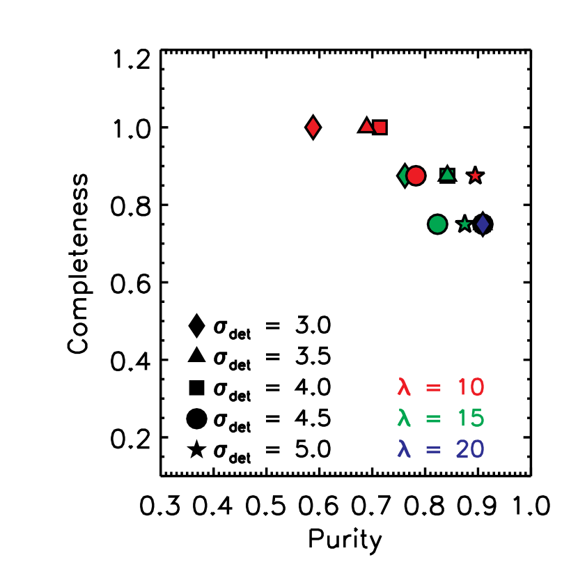
Figure 8: Completeness as a function of the purity for different thresholds of $\lambda$ and $\sigma_{det}$ up to $z\sim 0.6$ for the full Gozaliasl et al. (2014) sample. Red, green and blue symbols represent $\lambda\geq 10,15,20$ while diamonds, triangles, squares, circles and stars indicate $\sigma_{det}\geq 3,3.5,4,4.5,5$, respectively.

In this case, the completeness is estimated with respect to the X–ray detected catalogue from Gozaliasl et al. (2014) as the ratio between the number of X–ray detected clusters with $M_{200}\geq 10^{14}\ {\rm M_{\odot}}$ recovered by RedGOLD to the total number of X–ray detections with $M_{200}\geq 10^{14}\ {\rm M_{\odot}}$. Similarly, the purity is the ratio between the number of detections found by RedGOLD with an X–ray counterpart in the Gozaliasl’s catalogue to the total number of the RedGOLD detections. Our estimated purity is a lower limit, because the Gozaliasl’s catalogue purity and completeness are not published, and, as we show below, their catalogue is not complete at their mass limit. To optimise these two quantities, we test different values of each parameters and we retain those that maximise both completeness and purity.

To match the RedGOLD cluster candidates with the X-ray detected catalogue by Gozaliasl et al. (2014), we adopt a maximum projected distance between the centres corresponding to $R_{200}+\sigma_{R200}$, where $\sigma_{R200}$ is the estimated error on the $R_{200}$ measurement. Moreover, we require that the maximum redshift difference is $\Delta z=|z_{Goz}-z_{RedGOLD}|\leq 3\times\sigma_{photoz}=3\times 0.03\times(1+z)$, where $z_{Goz}$ is the cluster redshift in the Gozaliasl et al. (2014) catalogue and $z_{RedGOLD}$ is the cluster redshift estimated by RedGOLD.

Fig. 8 shows the estimated completeness as a function of the purity up to $z\sim 0.6$, while Fig. 9 shows the results estimated in the whole redshift range, for different limits on $\lambda$ and $\sigma_{det}$. Red, green and blue colours refer to $\lambda\geq 10,15,20$, respectively, while diamonds, triangles, squares, circles and stars refer to $\sigma_{det}\geq 3,3.5,4,4.5,5$, respectively. For low values of $\lambda$ and $\sigma_{det}$, the completeness is higher but the purity reaches lower values. For $z\lesssim 0.6$, the optimal values of $\lambda\geq 10$ and $\sigma_{det}\geq 4$ keep the completeness at $\sim 100\%$ and the purity at $>70\%$.

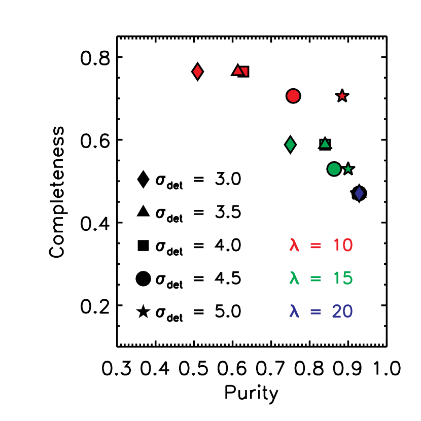
Figure 9: Completeness as a function of the purity for different thresholds of $\lambda$ and $\sigma_{det}$ in the whole redshift range for the full Gozaliasl et al. (2014) sample. Symbols are as in Fig. 8.

When considering the entire redshift range, $\lambda\geq 10$ and $\sigma_{det}\geq 4.5$ are the best values to obtain a completeness of $\sim 70\%$ and a purity of $\sim 80\%$, and the estimated completeness is lower than that estimated at $z\leq 0.6$. This is expected since half of the X–ray detections in the Gozaliasl’s catalogue with $M_{200}\geq 10^{14}\ {\rm M_{\odot}}$ is at $z\gtrsim 0.6$ and RedGOLD is expected to have a lower completeness at high redshift at the CFHTLenS depth, as shown in the previous section. The Gozaliasl’s sample does not include clusters at redshift $0.6<z<0.8$, for masses $M_{200}\geq 10^{14}\ {\rm M_{\odot}}$. For this reason, our lower redshift analysis stops at $z\sim 0.6$. Since we do not know the completeness of the Gozaliasl’s catalogue, our estimated purity is a lower limit. As an example, one RedGOLD detection without an X–ray counterpart in the Gozaliasl’s catalogue is a spectroscopically confirmed structure at $z=0.33$ (Andreon et al., 2004). Taking into account this detection, we recover a lower limit for the purity of $\sim 80\%$ at $z\leq 0.6$.

This analysis shows that our RedGOLD detections are optimised in both completeness and purity for $\lambda\geq 10$ and $\sigma_{det}\geq 4$ at $z\leq 0.6$, $\lambda\geq 10$ and $\sigma_{det}\geq 4.5$ for the higher redshifts. For this parameter choice, our RedGOLD catalogue is expected to be $100\%$ and $70\%$ complete, at $z\leq 0.6$ and $0<z<1.1$, respectively, and $\sim 80\%$ pure, for $M_{200}\gtrsim 1\times 10^{14}\ {\rm M_{\odot}}$. These results are consistent with the limits in $\sigma_{det}$ that we obtain from the Millennium Simulations for clusters with masses $M_{halo}\gtrsim 1\times 10^{14}\ {\rm M_{\odot}}$. We also note that our threshold $\lambda_{min}=10$, to obtain at least 10 bright galaxies within the scale radius, is in agreement with the literature (e.g., Eisenhardt et al., 2008).

We build our cluster catalogue considering $\lambda\geq 10$ and $\sigma_{det}\geq 4$ at $z\leq 0.6$, $\lambda\geq 10$ and $\sigma_{det}\geq 4.5$ for the higher redshifts. If the reader is interested in different values of completeness and purity, we advice to change the cuts in $\lambda$ and $\sigma_{det}$.

6 RedGOLD cluster candidate detections in the CFHT-LS W1 area

6.1 RedGOLD detections

Figure 10: Spatial distribution of the RedGOLD CFHT-LS W1 cluster candidate detections in the $\sim 60\ {\rm deg^{2}}$.

After applying our detection algorithm with $\lambda\geq 10$ and $\sigma_{det}\geq 4$ at $z\leq 0.6$, $\lambda\geq 10$ and $\sigma_{det}\geq 4.5$ at $z>0.6$, RedGOLD finds 652 detections with $\lambda\geq 10$ up to $z\sim 1.1$ in the $\sim 60\ {\rm deg^{2}}$ of the CFHT-LS W1 field, i.e. $\sim 11$ detections per $\rm deg^{2}$, of the same order of magnitude of theoretical predictions (Weinberg et al., 2013). Fig. 10 shows the spatial distribution of the CFHT-LS W1 detections up to redshift $z\sim 1$. Fig. 11 shows two of our richest cluster candidates at $z_{cluster}=0.19$ ($\lambda=80.5$) and at $z_{cluster}=0.44$ ($\lambda=54.1$).

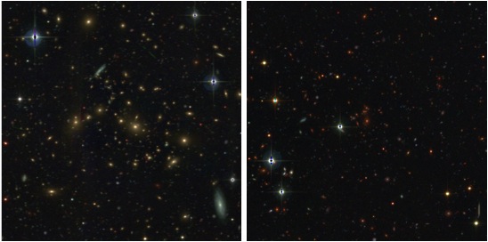
Figure 11: Optical images of two cluster candidates detected by RedGOLD at redshift $z_{cluster}=0.19$ (left panel) and $z_{cluster}=0.44$ (right panel). Their detection significance and richness are of $\sigma_{det}=8.6$ and $\lambda=80.5$, and $\sigma_{det}=11.1$ and $\lambda=54.1$, respectively.

In $\sim 18\ {\rm deg^{2}}$ of the area analysed in this work, published spectroscopy is available from the SDSS, VVDS and VIPERS surveys. We find that $\sim 58\%$ of the cluster candidates found in the same area, imposing these lower limits on the cluster richness and the detection level, have at least one spectroscopic member in less than $1.5^{\prime}$ with $|z_{spec}-z_{cluster}|<0.1$.

For each detection, we estimate its richness as described in section 4.4. The presence of saturated objects (stars and bright galaxies) leads to larger uncertainties on galaxy photometry, and as a consequence, on photometric redshifts. To take this into account, we use the photometric error distribution in each magnitude bin from Raichoor et al. (2014), and we exclude from the richness calculation galaxies with photometric errors larger than the average uncertainty plus three times its standard deviation (in each magnitude bin).

To test that this procedure does not significantly underestimate our richness, for each detected cluster candidate, we estimate the richness $\lambda_{mask}$, including also sources that are not included in our richness estimate because have large photometric errors in the Raichoor et al. (2014) CFHTLenS photometric catalogue.

Less than $7\%$ of the RedGOLD cluster candidates (obtained without imposing our lower limits on $\lambda$, $\sigma_{det}$ and the radial galaxy distribution) have a fraction of masked bright potential cluster members $>10\%$. These cluster candidates are very small systems with a mean redshift $\bar{z}_{cluster}=0.7$ and a mean richness $\bar{\lambda}_{mask}\sim 8$. If we consider only the RedGOLD detections obtained imposing our lower limits, we find that $\sim 2$% have a fraction of masked bright potential cluster members $>10\%$. These detections are also small structures at high redshift, with a mean richness $\bar{\lambda}_{mask}=12$ and mean redshift $\bar{z}_{cluster}=0.7$. This means that our richness estimate is not significantly affected by the presence of the CFHTLenS masks for at least $\sim 98$% of the cluster candidates in our final catalogue, and the fraction of masked members impacts our richness measurements only at low richness and high redshift.

Our catalogue includes: RA and DEC, the cluster redshift, the detection significance $\sigma_{det}$, the cluster richness $\lambda$ and the corresponding uncertainty $\lambda_{err}$.

In the next sections, we compare our detections with already published cluster catalogues.

6.2 Comparison with X–ray detected cluster catalogues

X–ray detected cluster catalogues in the same area include: (1) the X–ray group catalogue provided by Gozaliasl et al. (2014) in a subarea in the CFHT-LS W1 field; (2) the X–ray catalogue provided by Mehrtens et al. (2012), and (3) a sample of 33 spectroscopically confirmed X–ray detected clusters.

6.2.1 Comparison with the X–ray catalogue by Gozaliasl et al. (2014)

We have already shown the performance of RedGOLD in terms of purity and completeness with respect to the Gozaliasl et al. (2014) sample in section 5.3. The Gozaliasl et al. (2014) catalogue includes 135 X–ray clusters and groups in 3 deg² in the CFHT-LS W1 area. In the area covered by the Gozaliasl et al. (2014) catalogue, RedGOLD detects 38 cluster candidates, using the parameters optimised for the best simultaneous completeness and purity ($\lambda\geq 10$ and $\sigma_{det}\geq 4$ at $z\leq 0.6$, $\lambda\geq 10$ and $\sigma_{det}\geq 4.5$ at $z>0.6$), and imposing an NFW profile. Of those, 28 clusters are in the Gozaliasl et al. (2014) catalogue.

We cannot exclude that our additional ten detections without any X–ray counterpart are real galaxy groups, undetected in the X–rays. In fact, from visual inspection, they appear to be smaller systems and could have an X–ray emission below the X–ray detection limit or without X–ray emission, if they are not-relaxed systems. As pointed out in section 5.3, this is the case of a spectroscopically confirmed structure at $z\sim 0.3$ (Andreon et al., 2004), which is the richest RedGOLD detection without an X–ray counterpart. The 9 remaining detections have $\lambda<20$.

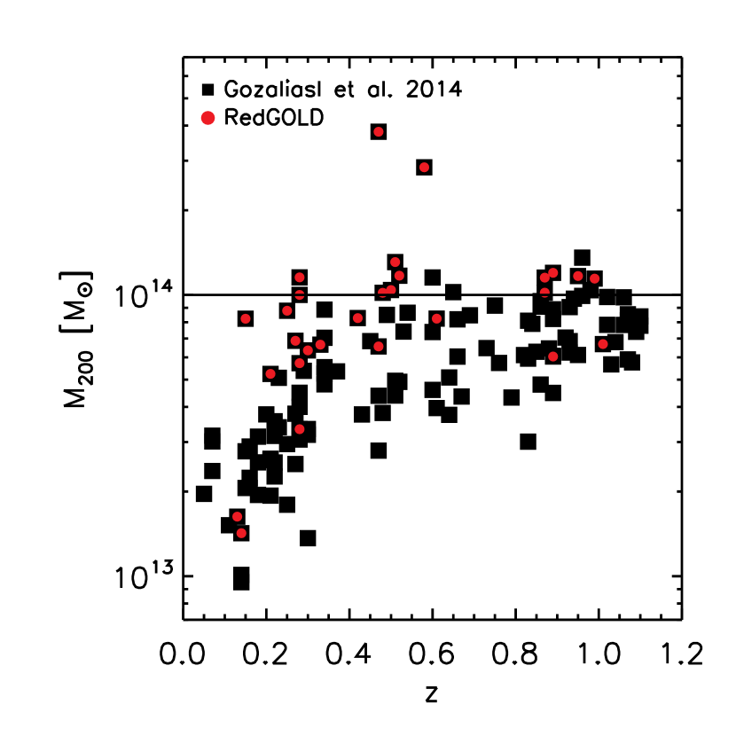
Figure 12: Cluster mass as a function of the redshift for the X–ray detected clusters from Gozaliasl et al. (2014) (black squares) and for the RedGOLD detections with an associate X–ray counterpart (red circles). The black solid line shows the $10^{14}\ {\rm M_{\odot}}$ mass limit.

Fig. 12 shows the cluster mass distribution as a function of the redshift for the X–ray detections from Gozaliasl et al. (2014) (black squares) and the clusters recovered by RedGOLD (red circles). The black solid line indicates the mass limit $M_{200}\geq 10^{14}\ {\rm M_{\odot}}$. RedGOLD detects 13 of the 17 X–ray detections with $M_{200}\geq 10^{14}\ {\rm M_{\odot}}$, in the entire redshift range, and all clusters with $z<0.6$ (completeness of $\sim 100\%$) in this mass range. As already discussed in section 5.3, this corresponds to a purity of $\sim 80\%$, and a completeness of $100\%$ and $70\%$, at $z\leq 0.6$ and $0.6<z<1.1$, respectively, for $M_{200}\gtrsim 10^{14}\ {\rm M_{\odot}}$.

We examined the four unrecovered structures with $M_{200}\geq 10^{14}\ {\rm M_{\odot}}$. All of them are at $z\geq 0.6$. Two of the unrecovered X–ray detections at $z=0.65$ and $z=0.6$ appear to be optical poor systems. The other two are at higher redshift, at z=0.96 and z=0.98, with masses $M_{200}=1.4\pm 0.2\times 10^{14}\ {\rm M_{\odot}}$ and $M_{200}=1.0\pm 0.2\times 10^{14}\ {\rm M_{\odot}}$, respectively, where we expect our algorithm to be $\sim 65\%$ complete for our choice of parameters (see section 5.3).

Redshift	$N_{Gozaliasl}$	Cluster Mass	% All Matched	% With lower limits on $\lambda$ and $\sigma_{det}$
$z<0.6$	8	$\geq 10^{14}\ {\rm M_{\odot}}$	$100\%$	$100\%$
	16	$\geq 7\times 10^{13}\ {\rm M_{\odot}}$	$75\%$	$69\%$
	60	$<7\times 10^{13}\ {\rm M_{\odot}}$	$20\%$	$15\%$
$z\geq 0.6$	9	$\geq 10^{14}\ {\rm M_{\odot}}$	$56\%$	$56\%$
	33	$\geq 7\times 10^{13}\ {\rm M_{\odot}}$	$24\%$	$18\%$
	26	$<7\times 10^{13}\ {\rm M_{\odot}}$	$15\%$	$8\%$

Table 1: Comparison of our detections with the X–ray catalogue by Gozaliasl et al. (2014).

Table 1 summarises our results, listing the RedGOLD detections in the two different redshift bins for the different mass limits, without imposing any constraints on $\lambda$ and $\sigma_{det}$ in the fourth column, and considering the optimal values for the RedGOLD parameters in the last column (see section 5.3).

6.2.2 Comparison with the X–ray catalogue by Mehrtens et al. (2012)

We compare our detections also with the X–ray cluster catalogue by Mehrtens et al. (2012).

There are 27 X–ray cluster detections from Mehrtens et al. (2012) in the region that we have analysed, 20 have a temperature measurement. We will consider these 20 for our analysis.

As for the Gozaliasl et al. (2014) catalogue, to match the RedGOLD cluster candidates with the X-ray detected catalogue by Mehrtens et al. (2012), we adopt a maximum projected distance between the centres corresponding to $R_{200}+\sigma_{R200}$ and a maximum redshift difference of $\Delta z=|z_{Meh}-z_{RedGOLD}|\leq 3\times\sigma_{photoz}=3\times 0.03\times(1+z)$, where $z_{Meh}$ is the cluster redshift in the Mehrtens et al. (2012) catalogue.

RedGOLD recovers 16 of the 20 Mehrtens et al. (2012) clusters, and their temperature ranges over $1<T_{X}<7.5$ keV (their median temperature is $T_{X}=4.1$ keV), without applying any constraints on $\lambda$, $\sigma_{det}$ and the radial galaxy distribution. We discard two detections adopting the optimal values of the cluster richness and the sigma detection level, for a final recovery of $70\%$($80\%$) of their detections with (without) limits.

Fig. 13 shows the redshift–$T_{X}$ distribution of the clusters in the Mehrtens et al. (2012) catalogue (orange squares), our recovered detections with and without imposing our lower limits in red and black, respectively. The four undetected clusters have low temperatures ($T_{X}=0.6-2.3$ keV) as shown in Fig. 15, i.e. are poor clusters or groups. We recover 11(13) of the 13 clusters with $T_{X}>2.5$ keV, i.e. the $85(100)\%$ of the X–ray detected clusters by Mehrtens et al. (2012) with (without) considering the RedGOLD lower limits.

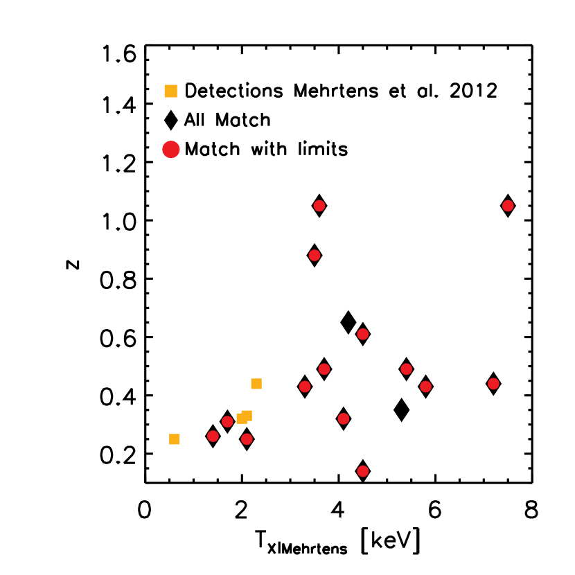
Figure 13: X–ray temperature $T_{X}$ as a function of the redshift $z$ for the clusters detected by RedGOLD with an X–ray counterpart in the Mehrtens et al. (2012) catalogue with a temperature estimate. The red circles and black diamonds represent the detections when considering or not the lower limits on the cluster richness, the detection significance and the radial galaxy distribution, respectively. The orange squares represent the four detections in the Mehrtens et al. (2012) catalogue that we do not recover with RedGOLD. The performance of RedGOLD are very encouraging, with only four unmatched detections of the Mehrtens et al. (2012) catalogue, all with $T_{X}\leq 2.3$ keV.

6.2.3 The temperature–richness relation

In this section, we discuss the scaling relation between optical and X–ray mass proxies, i.e. between the optical richness obtained with RedGOLD and the cluster X-ray temperature.

As already pointed out by Vikhlinin et al. (2006) and Rasia et al. (2006), the $\beta$–model does not accurately describe the cluster gas profile. This implies that the cluster masses estimated assuming a $\beta-$profile might be systematically underestimated up to a factor of $\sim 40\%$ both when considering the isothermal and polytropic laws for the cluster temperatures (Rasia et al., 2006).

For this reason, we do not use the mass measurements to study scaling relations, but we study directly the optical richness–$T_{X}$ relation. We use our recovered cluster detections up to $z=0.6$ in the Gozaliasl et al. (2014) catalogue to study the temperature–richness relation and compare our results with Rozo & Rykoff (2014).

We fit the $T_{X}$–$\lambda$ relation in the following way:

$$\ln(T_{X})=A+\alpha\ln(\lambda/\lambda_{pivot})\ ,$$ (6)

where $\lambda_{pivot}=median(\lambda)$, following (Rozo & Rykoff, 2014).

Fig. 14 shows the temperature–richness relation for the 20 galaxy clusters detected by RedGOLD in the CFHT-LS W1 field with a temperature measurement from Gozaliasl et al. (2014) up to $z=0.6$. Following Eq. 6, we perform a weighted fit on the errors and we obtain $A=0.34\pm 0.17$, $\alpha=0.82\pm 0.19$, $\lambda_{pivot}=20.47$ and the scatter $\sigma=0.28\pm 0.04$.

Assuming Eq. 2 from Rozo & Rykoff (2014) to estimate the scatter of the mass at fixed $\lambda$, we find a scatter of $\sigma_{M|\lambda}=0.39\pm 0.07$. The values of the amplitude, slope and mass scatter at fixed richness inferred by the fit are shown in the plot. We show the mean errors on the richness and temperature in the bottom right corner.

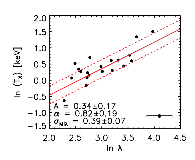
Figure 14: X–ray temperature $T_{X}$ as a function of the richness $\lambda$ (i.e. the $T_{X}-\lambda$ relation) for the 20 galaxy clusters detected by RedGOLD in the CFHT-LS W1 in common with the X–ray catalogue by Gozaliasl et al. (2014) up to $z=0.6$. We show the mean errors on the richness and the temperature in the bottom right corner.

We conduct the same analysis using the temperature measurements provided by Mehrtens et al. (2012). Fig. 15 shows the temperature–richness relation for the 8 galaxy clusters detected by RedGOLD in the CFHT-LS W1 field with a temperature measurement from Mehrtens et al. (2012) and a temperature error less than 30% up to $z=0.6$, following Rozo & Rykoff (2014). Performing a weighted fit on the errors to study the temperature–richness relation, we find that $A=1.42\pm 0.30$, $\alpha=1.54\pm 0.35$, $\lambda_{pivot}=35.38$ and a scatter $\sigma=0.22\pm 0.08$. Assuming Eq. 2 from Rozo & Rykoff (2014) to estimate the scatter of the mass at fixed $\lambda$, we find $\sigma_{M|\lambda}=0.30\pm 0.13$. As in Fig. 14, the values of the amplitude, slope and mass scatter at fixed richness inferred from the fit are shown in the plot.

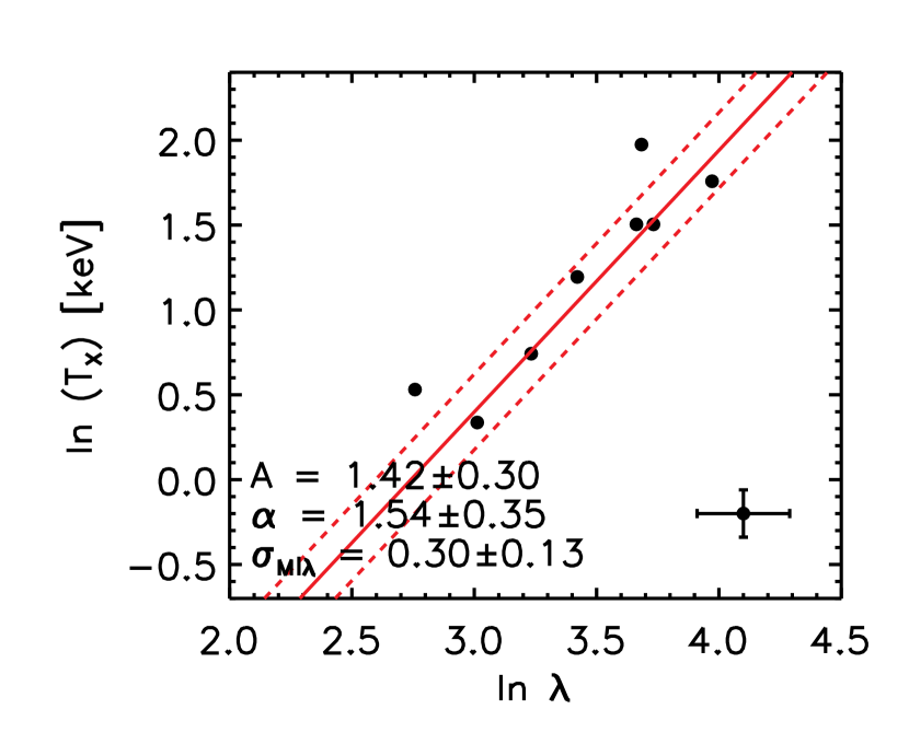
Figure 15: X–ray temperature $T_{X}$ as a function of the richness $\lambda$ (i.e. the $T_{X}-\lambda$ relation) for the 8 galaxy clusters detected by RedGOLD in the CFHT-LS W1 in common with the X–ray catalogue by Mehrtens et al. (2012) up to $z=0.6$. We show the mean errors on the richness and temperature in the bottom right corner.

Using the SDSS data and limiting the analysis to the redshift range $0.1<z<0.5$, Rozo & Rykoff (2014) found $A=1.206\pm 0.044$, $\alpha=0.57\pm 0.10$, $\sigma=0.225\pm 0.042$ and $\sigma_{M|\lambda}=0.30\pm 0.07$. The values of the slope for our fit to the Gozaliasl et al. (2014) temperatures are consistent with Rozo & Rykoff (2014) within $\approx 1\sigma$ while for the slope estimated using the Mehrtens et al. (2012) catalogue, our estimate is consistent with Rozo & Rykoff (2014) within 2$\sigma$. The scatter in mass at fixed richness obtained with the Gozaliasl et al. (2014) catalogue is comparable with Rozo & Rykoff (2014) but slightly higher while for the Mehrtens et al. (2012) catalogue we obtain the same value $\sigma_{M|\lambda}=0.3$.

The amplitude $A$ is significantly different when using the Gozaliasl et al. (2014) and Mehrtens et al. (2012) catalogues. For the fit to the Mehrtens et al. (2012) temperatures, the $A$ is consistent with Rozo & Rykoff (2014), while the $A$ for Gozaliasl et al. (2014) is significantly lower than both the Rozo & Rykoff (2014) and our fit to Mehrtens et al. (2012). The difference in the recovered amplitude of the temperature–richness relation is in part due to the different $\lambda_{pivot}$ for the two catalogues and to the different X–ray temperature definitions (e.g. see Rozo & Rykoff, 2014). While Gozaliasl et al. (2014) used core-excised temperatures, Mehrtens et al. (2012) did not. Using our scaling relations and Gozaliasl’s $M_{200}$, a temperature of $T_{X}\sim 1.8$ keV in the Gozaliasl’s catalogue corresponds to $M_{200}\sim 10^{14}\ \rm M_{\odot}$, and to a $\lambda\sim 30$. At this $\lambda$, the corresponding temperature in the Mehrtens et al. (2012) catalogue is $T_{X}\sim 2.7$ keV.

We are not able to investigate any evolution of the temperature–richness relation as a function of the redshift because of the small number of X–ray objects in the area.

These results are very promising because we are considering a lower richness threshold (i.e. lower cluster mass) with respect to the Rozo & Rykoff (2014) cluster sample (see section  6.3.1) and are obtaining similar scatters. If, instead of using all the X–ray clusters in our area, we consider only higher richness thresholds, corresponding to $M_{200}\sim 7\times 10^{13}\ \rm M_{\odot}$ ($M_{200}\sim 10^{14}\ \rm M_{\odot}$), we obtain a scatter in mass at fixed richness $\sigma_{M|\lambda}=0.27\pm 0.08\ (0.27\pm 0.16)$ and $\sigma_{M|\lambda}=0.24\pm 0.12\ (0.24\pm 0.24)$ estimated from the Gozaliasl et al. (2014) and the (Mehrtens et al., 2012) catalogue, respectively. However, when considering these higher richness thresholds we only have between five and ten clusters to perform the fit and, for this reason, we will need to analyse a larger cluster sample to confirm these results.

6.2.4 Spectroscopically confirmed X–ray clusters

We also compare our results to a subsample of spectroscopically confirmed X–ray groups and clusters (Pierre et al., 2006; Valtchanov et al., 2004; Andreon et al., 2004, 2005; Pacaud et al., 2007; Miyazaki et al., 2007; Olsen et al., 2007; Bergé et al., 2008). In the CFHT-LS W1 area there are 33 spectroscopically confirmed groups/clusters between $0.1<z<1.1$. In Table 2, we show the cluster ID, RA, DEC, redshift, and the corresponding reference for the spectroscopically confirmed clusters in the field.

To match the RedGOLD detections with the spectroscopically confirmed clusters, we adopt the same matching algorithm described for the X–ray detected catalogue, with a maximum projected distance between the centres corresponding to $R_{200}+\sigma_{R200}$ and a maximum redshift difference of $\Delta z=|z_{spec}-z_{RedGOLD}|\leq 3\times\sigma_{photoz}=3\times 0.03\times(1+z)$, where $z_{spec}$ is the cluster spectroscopic redshift.

Cluster ID	RA	DEC	z	Reference
XXLSSC 001	36.23792	-3.81472	0.614	(1)
XXLSSC 002	36.38542	-3.91944	0.772	(1)
XXLSSC 004	36.36833	-5.11583	0.88	(1)
XXLSSC 005	36.79042	-4.30139	1.0	(1)
XXLSSC 006	35.44083	-3.76889	0.429	(2)
XXLSSC 008	36.33417	-3.80833	0.297	(2)
RzCS 001	36.01792	-5.28944	0.494	(2)
XXLSSC 012	37.11417	-4.4300	0.433	(2)
XXLSSC 013	36.85792	-4.5375	0.307	(2)
XXLSSC 014	36.64375	-4.06528	0.344	(2)
XXLSSC 016	37.11750	-4.99611	0.332	(2)
XXLSSC 017	36.61417	-4.99861	0.381	(2)
XXLSSC 018	36.00667	-5.09028	0.322	(2)
XXLSSC 019	36.04917	-5.37972	0.494	(2)
XXLSSC 020	36.63667	-5.00889	0.494	(2)
XXLSSC 022	36.91667	-4.85806	0.29	(4)
XXLSSC 025	36.35292	-4.67861	0.26	(4)
XXLSSC 027	37.01417	-4.85083	0.29	(6)
XXLSSC 029	36.01625	-4.22444	1.05	(3)
VVDS Cluster	36.28917	-4.54833	0.77	(8)
XXLSSC 038	36.85417	-4.18972	0.58	(4)
XXLSSC 044	36.13958	-4.23472	0.26	(4)
XXLSSC 049	35.98917	-4.58806	0.49	(6)
XXLSSC 053	36.12167	-4.82333	0.49	(5)
XXLSSC 007	36.03750	-3.91917	0.557	(2)
XXLSSC 040	35.52292	-4.54639	0.32	(6)
XXLSSC 041	36.37833	-4.23972	0.14	(4)
a	36.34583	-4.44444	0.46	(4)
b	36.37333	-4.42972	0.92	(4)
c	36.54125	-4.52222	0.82	(4)
d	36.71625	-4.16583	0.34	(4)
XLSSCJ022534.2-042535	36.3925	-4.42639	0.92	(3)
XXLSSC 005b	36.8	-4.23056	1.0	(3)

Table 2: List of the confirmed galaxy clusters in the CFHT-LS W1. (1) Valtchanov et al. (2004), (2) Andreon et al. (2004), (3) Andreon et al. (2005), (4)Pierre et al. (2006), (5) Miyazaki et al. (2007), (6) Pacaud et al. (2007), (7) Bergé et al. (2008), (8) Le Fèvre et al. (2013).

RedGOLD recovers 24 out of the 33 spectroscopically confirmed clusters without considering any lower limit on $\lambda$, $\sigma_{det}$ and the radial galaxy distribution. When adopting the lower limits on $\lambda$, $\sigma_{det}$ and assuming the radial galaxy distribution, we discard 5 detections because of the imposed constraints on $\lambda$ (they all have $\lambda<10$). We check the nine missing detections: four detections are C2 and C3 objects from Pierre et al. (2006). This class includes faint and poor galaxy structures and their detection implies higher contamination rate.

A cluster at z=1 (ID=XLSS005b) is undetected by RedGOLD because it is blended with XLSSC005 at approximately the same redshift. An X–ray detected cluster at $z=0.92$ unrecovered by RedGOLD is an extremely poor system, undetected in $(R-z^{\prime})$, but appearing as a galaxy overdensity in the K–band, as found by Andreon et al. (2005). Finally, we are not able to recover three clusters at $z=0.322$, $z=0.381$ and $z=0.557$: the first one has a central BCG, but there is no a clear red overdensity, the second one is detected also in the catalogue by Gozaliasl et al. (2014) and has $M=8.5\pm 0.7\times 10^{13}\ {\rm M_{\odot}}$, and the last one is an optically poor system.

Figure 16: Left panel: the $(z_{spec}-z_{RedGOLD})$ distribution for the 19 spectroscopically confirmed clusters recovered by RedGOLD. The redshift difference is less than 0.05 for all detections up to $z\sim 1$. Right panel: $(z_{spec}-z_{RedGOLD})$ as a function of the spectroscopic redshift.

The comparison of our detection algorithm with these known X–ray detections on the CFHT-LS W1 confirms that the adopted cluster centre definition is efficient: in fact, the mean separation between the optical and the X–ray centre is $17.2^{\prime\prime}\pm 11.2^{\prime\prime}$ for all recovered confirmed clusters.

Up to redshift $z\sim 1$, we accurately recover the cluster redshift. In fact, the discrepancy between our cluster photometric redshifts and the corresponding spectroscopic measurement is less than 0.05, as shown is Fig.16, where the median $\delta z\sim 0.004$. The right panel of Fig.16 shows that the redshift difference $(z_{spec}-z_{RedGOLD})$ is larger at higher redshift (i.e. $z\geq 0.5$), with four out of six objects with $|z_{spec}-z_{RedGOLD}|>0.02$. This is expected since the photometric redshift accuracy is lower at fainter magnitudes and increasing redshifts. However, this effect is negligible, being the redshift difference $|z_{spec}-z_{RedGOLD}|$ very low for all the spectroscopic confirmed clusters recovered by RedGOLD. This result confirms that the BC03 model colours (from which we derive $z_{RedGOLD}$) accurately reproduce galaxy colours in the redshift range that we considered.

From Bergé et al. (2008), we have a mass estimate based on weak lensing measurements for four clusters detected by RedGOLD in the XMM-LSS area: we recover all the four clusters in the CFHT-LS W1 field. We show these values in Table 3.

XLSSC	RA	Dec	z	$M_{200}$ (WL)
	$(^{\circ})$	$(^{\circ})$		$(10^{13}{\rm h^{-1}M_{\odot}})$
013	36.8497	-4.5481	0.307	$8.2^{+2.5}_{-1.9}$
053	36.1229	-4.8341	0.50	$10.3^{+3.0}_{-2.6}$
041	36.3723	-4.2604	0.14	$4.9^{+1.6}_{-1.2}$
044	36.1389	-4.2384	0.26	$7.2^{+2.3}_{-1.7}$

Table 3: Mass estimates for 4 clusters in the XMM-LSS area from Bergé et al. (2008). We recover all 4 clusters.

6.3 Comparison with optically selected cluster catalogues

Three optically detected cluster catalogues are publicly available in the CFHT-LS W1 field: (1) the redMaPPer catalogue from Rykoff et al. (2014), obtained using SDSS observations; (2) the Milkeraitis et al. (2010) and the (3) Durret et al. (2011) catalogues, both obtained using CFHT-LS W1 observations and methods using photometric redshift catalogues.

6.3.1 Comparison with redMaPPer

The first optically detected cluster catalogue to which we compare the RedGOLD cluster candidates is the redMaPPer catalogue (Rykoff et al., 2014), obtained using observations from the SDSS. In Fig. 17, we show the redshift distribution of our cluster candidates: the red solid line represents the RedGOLD detections in the CFHT-LS W1 field while the dashed black line shows the redshift distribution of the redMaPPer catalogue in the same area. Both histograms are normalised to the total number of detections found by the corresponding algorithm. As expected, we detect cluster candidates at higher redshift than redMaPPer since the CFHTLenS data are deeper than the SDSS.

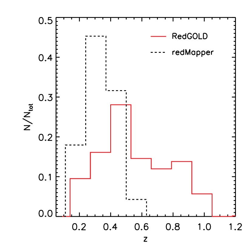
Figure 17: Redshift distribution of CFHT-LS W1 cluster detections in the $\sim 60\ deg^{2}$ (red solid line). The black dashed line represents the redMaPPer detections in the same region. Each histogram is normalised to the total number of detections.

To match the RedGOLD cluster candidates with the redMaPPer catalogue, we adopt the same matching algorithm described for the X–ray detected catalogue, with a maximum projected distance between the centres corresponding to $R_{200}+\sigma_{R200}$ and a maximum redshift difference of $\Delta z=|z_{redMaPPer}-z_{RedGOLD}|\leq 3\times\sigma_{photoz}=3\times 0.03\times(1+z)$, where $z_{redMaPPer}$ is the cluster redshift in the redMaPPer catalogue.

There are 116 redMaPPer cluster detections in our field, 115 detected with RedGOLD (i.e. the $99\%$), when not applying any lower limit on the radial galaxy distribution, $\lambda$ and $\sigma_{det}$. The only redMaPPer cluster that we do not detect has a sparse structure and has redshift $z=0.48$. We discard seven additional redMaPPer detections when considering the optimal lower limits imposed on the radial galaxy distribution (two detections) and richness and $\sigma_{det}$ (five detections). With this final selection, we obtain 108 RedGOLD detections out of the 116 clusters detected with redMaPPer (i.e. $\sim 93\%$).

All the redMaPPer detections in the area spanned by the Gozaliasl et al. (2014) catalogue, six clusters, have an X–ray counterpart. RedGOLD considers as detections only five of these six clusters. The unrecovered redMaPPer detection with an X–ray counterpart is at $z\sim 0.5$ and has $M_{200}\sim 8.5\times 10^{13}\ {\rm M_{\odot}}$, i.e. it is in the mass range in which we are $\sim 70\%$ complete (see section 5 and 6.2.1).

Fig. 18 shows the mass distribution of the clusters recovered by RedGOLD in red and those recovered by redMaPPer in black: our catalogue reaches lower cluster mass values with respect to the redMaPPer detections, as expected since the CFHTLenS is deeper than the SDSS, and the redMapper catalogue is cut at a given richness. For this reason, our RedGOLD catalogue includes $\sim 200$ detections up to $z=0.5$, unrecovered by redMaPPer using the SDSS.

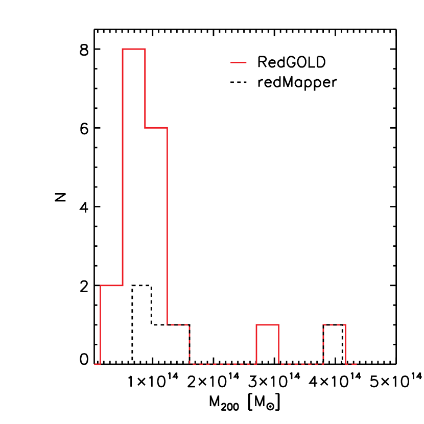
Figure 18: Mass distribution of the cluster detected by RedGOLD (red solid line) and redMaPPer (black dashed line) with an X–ray counterpart in the Gozaliasl et al. (2014) catalogue. The mass measurements are from Gozaliasl et al. (2014).

In Fig. 19 and Fig. 20, we compare the richness estimates obtained by redMaPPer and RedGOLD for the 108 common detections. We show the $\lambda_{RedGOLD}$ vs $\lambda_{redMaPPer}$ and the histogram of the difference between our richness definition and the richness adopted in Rykoff et al. (2014), ($\lambda_{redMaPPer}-\lambda_{RedGOLD}$)/($\lambda_{RedGOLD}$), in different redshift bins, respectively.

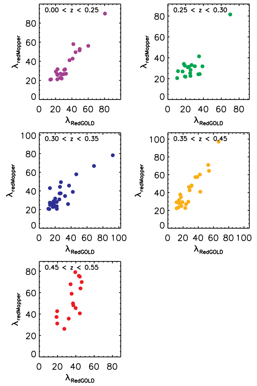
Figure 19: Comparison of the RedGOLD and redMaPPer richness, ($\lambda_{redMaPPer}$ vs $\lambda_{RedGOLD}$), in different redshift bins as indicated in each panel.

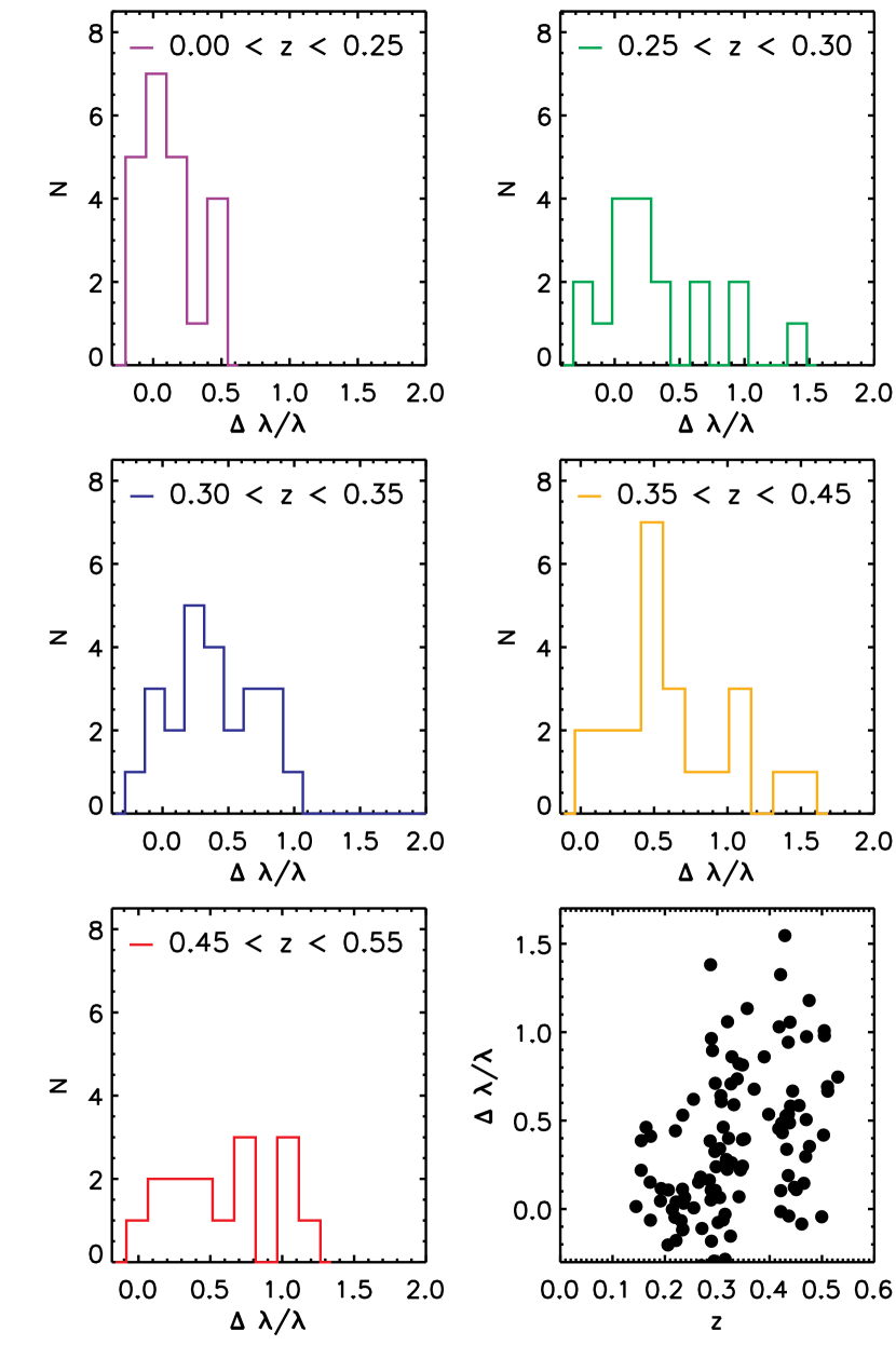
Figure 20: Histogram of the $\left(\frac{\lambda_{redMaPPer}-\lambda_{RedGOLD}}{\lambda_{RedGOLD}}\right)$, in different redshift bins as indicated in each panel. The bottom right panel shows the $\left(\frac{\lambda_{redMaPPer}-\lambda_{RedGOLD}}{\lambda_{RedGOLD}}\right)$ distribution as a function of the redshift.

Different colours show the observed difference in different redshift bins, as indicated in each panel. The redMaPPer richness is systematically higher than the RedGOLD richness as defined in this paper. In the bottom right panel in Fig. 20, we plot the ($\lambda_{redMaPPer}-\lambda_{RedGOLD})/\lambda_{RedGOLD}$ as a function of redshift: the difference between the two richness estimates in the RedGOLD and redMaPPer catalogue is larger at higher redshift. In Fig. 20, there is an apparent lack of clusters at z=0.35. This depends on the lack of galaxies at $z\sim 0.35$in the galaxy photometric redshift distribution. We check the galaxy photometric redshifts of the objects with a spectroscopic redshifts $0.3\lesssim z\lesssim 0.4$ and they are fully consistent with the spectroscopic measurements. Therefore, we conclude that the apparent lack of clusters visible in Fig. 20 is due the cosmic variance.

In Table 4, we present the median value of this richness difference as a function of redshift. The median difference is small at low redshift ($\sim 5-15\%$) at $z<0.3$, but it increases up to $\sim 60\%$ at higher redshifts (with single values reaching the $\sim 200\%$). At these redshifts, we keep a simple approach counting galaxies up to the depth reached by the CFHTLenS, while the redMaPPer richness estimate includes an extrapolation of the SDSS depth (which is lower than CFHTLenS) to our same limit in ${\rm L^{*}}$. It would be worth to investigate the observed difference richness in a future work, considering a larger cluster sample.

redshift	median($\Delta\lambda/\lambda_{RedGOLD}$)
$z\leq 0.25$	0.05
$0.25<z\leq 0.30$	0.16
$0.30<z\leq 0.35$	0.39
$0.35<z\leq 0.45$	0.54
$0.45<z\leq 0.55$	0.59

Table 4: Median value of $(\lambda_{redMaPPer}-\lambda_{RedGOLD})/\lambda_{RedGOLD}$ in different redshift bins

6.3.2 Comparison with other catalogues obtained with CFHT-LS W1 observations

Figure 21: Histogram of the RedGOLD sigma detection level $\sigma_{det}$ for the unrecovered detections in the catalogue provided by Milkeraitis et al. (2010) with $\sigma_{Milkeraitis}\geq 5$.

There are two public optically selected cluster candidate catalogues, obtained using the same CFHT-LS W1 observations as the CFHTLenS catalogue, the Milkeraitis et al. (2010) and the Durret et al. (2011) catalogues.

Milkeraitis et al. (2010) developed the 3D-Matched-Filter technique (3D-MF) to detect galaxy clusters, and applied it to the four wide fields of the CFHT-LS. Their detection algorithm is based on the matched filter technique, assuming a cluster radial profile and luminosity function. They used photometric redshifts to reduce contamination due to projection effects.

To compare our detections with the Milkeraitis et al. (2010) catalogue, we cut their catalogue to $\sigma_{Milkeraitis}\geq 5$, corresponding to $\sim 1.6\times 10^{13}\ {\rm M_{\odot}}$ (Ford et al., 2015), with an expected false detection rate $>30\%$ (Milkeraitis et al., 2010). We match the Milkeraitis et al. (2010) catalogue with the RedGOLD cluster candidates adopting less conservative constraints, with a maximum projected distance between the centres of 2 Mpc and a cluster redshift difference $|z_{Milkeraitis}-z_{RedGOLD}|\leq 0.2$, since the cluster redshift estimates in the Milkeraitis et al. (2010) catalogue are not refined and have a bin of 0.1.

In the CFTH-LS W1 subfield covered by this work, Milkeraitis et al. (2010) detected 2871 cluster candidates with $\sigma_{Milkeraitis}\geq 5$. Of those, RedGOLD detects 1753 objects ($61\%$), when not applying any lower limit on the radial galaxy distribution, $\lambda$ and $\sigma_{det}$. When considering the optimal lower limits imposed on the radial galaxy distribution, richness and $\sigma_{det}$, we discard 1158 objects, and obtain 595 RedGOLD detections (i.e., the $21\%$ of the Milkeraitis’ detections). These numbers are expected since we find $\sim 11$ detections per $\rm deg^{2}$ while Milkeraitis et al. (2010) found more than $45$ detections per $\rm deg^{2}$ at $\sigma_{Milkeraitis}\geq 5$.

To understand which kind of objects RedGOLD does not detect or discards, we estimate our detection level at the positions of the centres of the unrecovered detections of the Milkearitis’ catalogue. Fig. 21 shows the distributions of our estimated $\sigma_{det}$, corresponding to the unrecovered candidates in the Milkeraitis’ catalogue.

We find that only $\sim 3\%$ of the unrecovered Milkeraitis’ detections have a $\sigma_{det}\geq 4$ at $z\leq 0.6$ and $\sigma_{det}\geq 4.5$ at $z>0.6$: this implies that we do not select most of their detections because of their low $\sigma_{det}$. In fact, in this low $\sigma_{det}$ range, we expect a lower purity that we do not accept (see previous section). The remaining $\sim 3\%$ with a $\sigma_{det}$ in our selection range, are discarded because of their low $\lambda$. The median significance of the Milkeraitis’ discarded detections is $\sigma_{Milkeraitis}\sim 5$, which approximately corresponds to $M\sim 1.6\times 10^{13}\ {\rm M_{\odot}}$ (Ford et al., 2015).

It is interesting that, when we consider higher $\sigma_{Milkeraitis}$ detections, at $\sigma_{Milkeraitis}\geq 10$, which corresponds to $M\gtrsim 10^{14}\ {\rm M_{\odot}}$ (Ford et al., 2015), RedGOLD recovers the $\sim 78\%(95\%)$ of the objects with (without) the imposed criteria on the RedGOLD parameters. At $\sigma_{Milkeraitis}\geq 15$, RedGOLD recovers the $\sim 95\%(100\%)$ of the objects, at higher $\sigma_{Milkeraitis}>17$, we recover the same 13 objects with (without) the imposed criteria on the RedGOLD parameters. This means that for the most massive detections, we recover similar cluster candidates.

On the other hand, RedGOLD detects 652 cluster candidates and approximatively $75\%$ of those are also selected in the Milkeraitis’ catalogue when considering all their detections with $\sigma_{Milkeraitis}\geq 5$. When considering all objects in the Milkeraitis’ catalogue (i.e. $\sigma_{Milkeraitis}\geq 3.5$), we find $\sim 85\%$ of the RedGOLD detections.

Figure 22: Histogram of the RedGOLD sigma detection level $\sigma_{det}$ for the unrecovered detections in the catalogue provided by Durret et al. (2011) with $S/N\geq 3$ within the redshift range $0.375<z<1.05$.

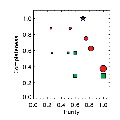
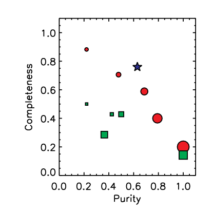
Figure 23: Completeness as a function of the purity for the Milkeraitis et al. (2010) (red circles) and Durret et al. (2011) (green squares) catalogues, respectively, estimated using the X–ray detected catalogue from Gozaliasl et al. (2014) sample. The size of the symbols shows different thresholds of their detection level: from the smaller to the larger $\sigma_{Milkeraitis}=3,5,6,8,10$ and $\sigma_{Durret}=2,4,5,6,7$. The left and right panels show results for $z<0.6$ and in the whole redshift range, respectively. The blue star represents the value of completeness and purity reached by RedGOLD with the optimised values of $\sigma_{det}$ and $\lambda$.

	Milkeraitis et al. (2010)	Durret et al. (2011)
$\sigma_{catalogue}<\sigma_{limit}$	68% (74%)	33% (42%)
$\sigma_{catalogue}\geq\sigma_{limit}$	32% (26%)	67% (58%)
$N_{common}/N_{tot}$	595(1753) / 2871	250 (732) / 1293
%$N_{common}/N_{tot}$	21% (61%)	19% (57%)
$N_{det}$	652 (3015)	475 (2440)
$N_{common}/N_{det}$	91% (58%)	53% (30%)

Table 5: Percentage of the matched cluster candidates from Milkeraitis et al. (2010) and Durret et al. (2011) obtained considering our detection limit $\sigma_{det}\geq 4$ at $z\leq 0.6$, and $\sigma_{det}\geq 4.5$ at $z>0.6$. For the comparison with Milkeraitis et al. (2010), we consider $\sigma_{Milkeraitis}\geq 5$, which correspond to $M>1.5\times 10^{13}\ {\rm M_{\odot}}$. The first and second row show the percentage of matched detections with $\sigma_{Milkeraitis}<10$ and $\sigma_{Milkeraitis}\geq 10$, which correspond to $M=10^{14}\ {\rm M_{\odot}}$ (Ford et al., 2015). For the comparison with Durret et al. (2011), we split their sample considering $\sigma_{Durret}<4$ and $\sigma_{Durret}\geq 4$. $N_{common}$ represents the number of the common detections (our minimum detection has $\sigma_{det}\geq 3$) while $N_{tot}$ is the total number of cluster candidates in their optical cluster catalogue. $N_{det}$ is the number of the cluster candidates detected by RedGOLD. The values in parenthesis refer to the comparison without applying any lower limit on the radial galaxy distribution, $\lambda$ and $\sigma_{det}$.

Durret et al. (2011) built an optical detected cluster catalogue, using a detection technique based on the galaxy density maps (Adami et al., 2010): they used photometric redshifts and detected overdensities in redshift slices, over a given threshold using the tool SExtractor (Bertin & Arnouts, 1996). For each detection, they provide the cluster candidate photometric redshift.

We match the Durret et al. (2011) catalogue with the RedGOLD cluster candidates adopting the same matching algorithm used for the Milkeraitis et al. (2010) cluster catalogue.

When comparing our detections to their catalogue, we only consider their most reliable detections, i.e. those in the redshift range $0.375<z<1.05$ and with a signal–to–noise ratio $S/N\geq 3$ (Durret et al., 2011). Those are 1293 objects and RedGOLD detects the $\sim 19\%$ (57%) of the objects with (without) the imposed criteria on the RedGOLD parameters.

As above, we estimate our sigma detection level $\sigma_{det}$ at the position of the unmatched Durret’s candidates and we show their distribution in Fig. 22. Also in this case, most of the missing detections have a low detection level, with only $3\%$ of the unrecovered Durret candidates having $\sigma_{det}\geq 4$ at $z\leq 0.6$ and $\sigma_{det}\geq 4.5$ at $z>0.6$: this implies that they are mostly lower $\sigma_{det}$ (i.e. less massive) detections.

If we consider the RedGOLD cluster candidate catalogue in the redshift range $0.35<z<1.1$ to match the Durret’s catalogue to our catalogue in the same redshift interval, we find 475 (2440) with (without) imposing our constraints on the RedGOLD parameters, but only $\sim 34\%$ ($\sim 19\%$) are detected also by Durret et al. (2011). The mean richness and detection significance of the RedGOLD cluster candidates not detected in the Durret’s catalogue are $<\lambda>\simeq 17\ (8)$ and $<\sigma_{det}>\simeq 6\ (4)$ when considering our cluster sample with (without) lower limits on the RedGOLD parameters.

From this comparison, we conclude that most of the Durret et al. (2011) cluster candidates are objects less massive than ours, and that their algorithm does not find most of our massive candidates.

We summarise our results on the comparison with the other optical detected cluster catalogues obtained with CFHT-LS W1 observations in Table 5 and Table 6.

Table 5 shows the distribution of their detection significances for the matched cluster candidates when applying the optimal values for $\lambda$ and $\sigma_{det}$ for the RedGOLD detections and considering the cluster candidates from the Milkeraitis et al. (2010) and Durret et al. (2011) catalogues, with $\sigma_{Milkeraitis}\geq 5$ and $\sigma_{Durret}\geq 3$, respectively. We show this distribution splitting the detection significances of the candidates recovered by RedGOLD with respect to $\sigma_{limit}=10$ and $\sigma_{limit}=4$, for the Milkeraitis et al. (2010) and Durret et al. (2011) catalogue, respectively. The corresponding values without imposing any lower limit on the RedGOLD parameters are shown in parenthesis. In Table  5, we also show the fraction $N_{common}/N_{tot}$, where $N_{common}$ is the number of the common detections and $N_{tot}$ is the total number of the cluster candidates in the two different cluster catalogues and the $N_{common}/N_{det}$ ratio, where $N_{det}$ is the number of the RedGOLD detections.

Table 6 shows the detection significance $\sigma_{det}$ for the unmatched cluster candidates from the two other catalogues that we analysed, the Milkeraitis et al. (2010) and Durret et al. (2011) catalogues, when we run RedGOLD on their detection centres. Depending on the algorithm, we find that $\sim 70-80\%$ of the unmatched candidates have RedGOLD detections at $<2\sigma$, and only $\sim 3\%$ have RedGOLD detections at $>4.5\sigma$.

As already described for the RedGOLD cluster candidates, we estimate the completeness and purity with respect to the Gozaliasl et al. (2014) catalogue for the Milkeraitis et al. (2010) and the Durret et al. (2011) detections. In Fig. 23, we show the completeness as a function of the purity for different detection levels, up to $z\sim 0.6$ (left panel) and in the whole redshift range (right panel). Red circles and green squares refer to the Milkeraitis et al. (2010) and Durret et al. (2011) catalogues, respectively. The size of the symbols shows different thresholds of their detection level: from the smaller to the larger $\sigma_{Milkeraitis}=3,5,6,8,10$ and $\sigma_{Durret}=2,4,5,6,7$.

As expected, the completeness decreases with the increasing detection level thresholds, and reaches $\sim 90\%$ at $\sigma_{Milkeraitis}\geq 3$ and $\sim 60\%$ at $\sigma_{Durret}\geq 2$ for the Milkeraitis et al. (2010) and Durret et al. (2011) catalogue, respectively. On the other hand, the purity increases with the detection significance: the best compromise between completeness and purity is found for $\sigma_{Milkeraitis}\geq 6$ and for $\sigma_{Durret}\geq 5$.

With this cut, the Milkeraitis et al. (2010) catalogue reaches a completeness of $\sim 75\%$ ($\sim 60\%$) at $z\leq 0.6$ ($z\leq 1.1$) and a purity of $\sim 75\%$ ($\sim 70\%$) at $z\leq 0.6$ ($z\leq 1.1$). Similarly, the Durret et al. (2011) catalogue reaches a completeness of $\sim 60\%$ ($\sim 40\%$) at $z\leq 0.6$ ($z\leq 1.1$) and a purity of $\sim 60\%$ ($\sim 50\%$) at $z\leq 0.6$ ($z\leq 1.1$). The blue star represents the value of completeness and purity reached by RedGOLD with the optimised values of $\sigma_{det}$ and $\lambda$.

This comparison shows that the RedGOLD catalogue reaches a better compromise between completeness and purity at both low and high redshifts with respect to the Milkeraitis et al. (2010) and Durret et al. (2011) catalogues, being more complete and purer when using our thresholds on $\lambda$ and $\sigma_{det}$.

RedGOLD	Milkeraitis et al. (2010)	Durret et al. (2011)
$\sigma_{det}<1$	45%	57%
$\sigma_{det}\geq 1$	55%	43%
$\sigma_{det}\geq 2$	29%	21%
$\sigma_{det}\geq 3$	11%	10%
$\sigma_{det}\geq 4$	4%	4%
$\sigma_{det}\geq 4.5$	2%	3%
$N_{tot}$	1425	1036

Table 6: Percentage of the unmatched cluster candidates for each detection limit when we run our algorithm on the cluster candidate centres from Milkeraitis et al. (2010) and Durret et al. (2011) with $\sigma_{det}<1$, $\sigma_{det}\geq 1$, $\sigma_{det}\geq 2$, $\sigma_{det}\geq 3$, $\sigma_{det}\geq 4$ and $\sigma_{det}\geq 4.5$. $N_{tot}$ represents the total number of the unmatched detections for each optical cluster catalogue.

7 Conclusions

We present our galaxy cluster detection algorithm RedGOLD and apply it to $\sim 60$ deg² of the optical survey CFHT-LS W1 to detect clusters up to $z\sim 1$ using the CFHTLenS data reduction. RedGOLD is based on a revised red–sequence overdensity search technique. To properly detect overdensities of passive red-sequence galaxies, we use colour-colour diagrams and color cuts that correspond to the $(U-B)$ and $(B-V)$ rest–frame colours of passive ETGs. This permits us to discard blue star-forming galaxies and dusty star-forming galaxies with the same $(U-B)$ rest–frame colour as passive galaxies at the same redshifts. Photometric redshifts improve our selection on the red–sequence, and the spectral classification from the SED fitting identifies ETGs. We also impose a constraint on the cluster profile, and RedGOLD only retains detections with a radial distribution in agreement with the NFW profile.

RedGOLD detections are characterised by their significance $\sigma_{det}$. The algorithm also provides the candidate richness $\lambda$ as a proxy of the cluster mass. We adopt the modification of the richness definition from Rykoff et al. (2014) for the redMaPPer algorithm applied to the SDSS, and adapt it to the CFHTLenS depth. We show that our richness $\lambda$ is very similar to the richness from Rykoff et al. (2014) up to $z\sim 0.3$. At higher redshift, the redMaPPer richness is systematically higher, up to a median difference of $\sim 60\%$. Because the CFHTLenS is deeper than the SDSS, we believe that this difference is partially due to the fact that we are counting galaxies down to the CFHTLenS depth, while in redMaPPer the richness estimate is extrapolated to a larger depth than the SDSS, but we will investigate this observed difference in a future work by analysing a larger cluster sample.

The detection significance $\sigma_{det}$ and the cluster richness $\lambda$ are the two key parameters for the completeness and purity of the RedGOLD cluster catalogues. We calibrate the optimal values of these two parameters using both simulations and X–ray observations from Gozaliasl et al. (2014). We apply RedGOLD to the Millennium Simulations, using the lightcones built by Henriques et al. (2012) based on the Guo et al. (2011) model. We find that the red–sequence of clusters in their lightcones is not accurately reproduced, with a lack of ETGs and bluer colours than those predicted by the BC03 models (which accurately reproduce the observed colours as a function of redshift). We modify the simulations to correct their biases in colour and ETG fractions.

From both our calibration on simulations and observations, we obtain the values of $\sigma_{det}$ and $\lambda$ that optimise completeness and purity at the same time: our final cluster catalogue in the CFHT-LS W1 includes candidates with $\lambda\geq 10$ and $\sigma_{det}\geq 4$ at $z\leq 0.6$, and $\sigma_{det}\geq 4.5$ at $z>0.6$. For cluster mass $M_{200}>10^{14}\ {\rm M_{\odot}}$, RedGOLD is $\sim 80\%$ pure up to $z\sim 1.1$. In this mass range, for $z\lesssim 0.6$ ($0.6<z<1.1$), the optimal values of $\lambda\geq 10$ and $\sigma_{det}\geq 4$ ($\lambda\geq 10$ and $\sigma_{det}\geq 4.5$) give us a completeness of $\sim 100\%$ ($\sim 70\%$).

In the CFHT-LS W1 area analysed in this work, and using the parameter range above, we find $\sim 11$ detections per $\rm deg^{2}$ up to $z\sim 1.1$. Approximatively $58\%$ of our detections have at least one galaxy with a confirmed spectroscopic redshift from public catalogues available in the area that is within the uncertainty of the cluster photometric redshift. The comparison of our detections with available X-ray detected cluster catalogs confirms our estimated completeness.

Our centring algorithm and our determination of the cluster photometric redshift are very precise: we find that the median separation between the peak of the X–ray emission and our cluster centres is $17.2^{\prime\prime}\pm 11.2^{\prime\prime}$, and the redshift difference with spectroscopy is less than 0.05 up to $z\sim 1$.

Comparing our catalogue with the redMaPPer detections from (Rykoff et al., 2014), we recover $\sim 99\%$ of their detections with no limits on $\lambda$ and $\sigma_{det}$. When applying the limits on the RedGOLD parameters, we discard 7 small systems, recovering $\sim 93\%$ of the detections in the redMaPPer catalogue. When comparing with redMaPPer detections which are also in the Gozaliasl et al. (2014) X–ray group catalogue, we find that RedGOLD recovers all the redMaPPer detections but one with $M_{200}=8.5\times 10^{13}\ {\rm M_{\odot}}$ at $z\sim 0.5$. Our cluster catalogue reaches lower cluster masses with respect to the redMaPPer detections. We believe that this is because the CFHTLenS is deeper than the SDSS and because the redMaPPer catalogue was built using a different limit in the cluster candidate richness.

We study the $T_{X}-\lambda$ relation for the RedGOLD detections using the Gozaliasl et al. (2014) and Mehrtens et al. (2012) X–ray catalogues. Up to $z=0.6$ and using the Gozaliasl et al. (2014) catalogue, for the relation $\ln(T_{X})=A+\alpha\ln(\lambda/\lambda_{pivot})$ we obtain $A=0.34\pm 0.17$, $\alpha=0.81\pm 0.20$ and a scatter of $\sigma=0.28\pm 0.04$, corresponding to a scatter in mass at fixed richness of $\sigma_{M|\lambda}=0.39\pm 0.07$. Using the Mehrtens et al. (2012) catalogue, we obtain $A=1.41\pm 0.32$, $\alpha=1.55\pm 0.75$ and a scatter $\sigma=0.23\pm 0.08$, corresponding to $\sigma_{M|\lambda}=0.30\pm 0.13$. Our results are consistent with Rozo & Rykoff (2014), when using both the Gozaliasl et al. (2014) and the Mehrtens et al. (2012) catalogue, even if we find a slightly higher scatter at fixed richness for the Gozaliasl et al. (2014) catalogue. This result is very promising because the RedGOLD catalogue reaches a lower mass threshold. If we apply richness cuts corresponding to $M_{200}\sim 7\times 10^{13}\ M_{\odot}$ and $M_{200}\sim\times 10^{14}\ M_{\odot}$, we obtain smaller values of the scatter in mass at fixed richness. However, with these higher richness thresholds we only have a small number of points, and we need to extend this analysis to a larger cluster sample.

We compare our RedGOLD cluster catalogue to two optical cluster catalogues publicly available in the same area, the Milkeraitis et al. (2010) and the Durret et al. (2011) catalogues. For cluster masses $M_{200}\gtrsim 10^{14}\ {\rm M_{\odot}}$, RedGOLD recovers $\sim 80\%$ of the Milkeraitis’ detections, and discards a significant fraction of small groups detected in the two catalogues. When we estimate the completeness and purity of these two algorithms, we obtain optimised values that are lower than those of RedGOLD at all redshifts. We find that the best compromise between completeness and purity is found for $\sigma_{Milkeraitis}\geq 6$ and for $\sigma_{Durret}\geq 5$. With this cut, the Milkeraitis et al. (2010) catalogue reaches a completeness of $\sim 75\%$ ($\sim 60\%$) at $z\leq 0.6$ ($z\leq 1.1$) and a purity of $\sim 75\%$ ($\sim 70\%$) at $z\leq 0.6$ ($z\leq 1.1$). Similarly, the Durret et al. (2011) catalogue reaches a completeness of $\sim 60\%$ ($\sim 40\%$) at $z\leq 0.6$ ($z\leq 1.1$) and a purity of $\sim 60\%$ ($\sim 50\%$) at $z\leq 0.6$ ($z\leq 1.1$). Comparing these three catalogues at their optimal values of completeness and purity, we find that RedGOLD is both more complete and purer than Milkeraitis et al. (2010) and Durret et al. (2011).

Our results show that our cluster detection algorithm RedGOLD is able to effectively detect galaxy clusters with mass $M\gtrsim 10^{14}\ {\rm M_{\odot}}$, with a purity of $\sim 80\%$ at $z\lesssim 1.1$, and a completeness of $\sim 100\%$ at $z\leq 0.6$, and $\sim 70\%$ up to $z\sim 1$, at the CFHTLenS depth.

References

- Adami et al. (2010) Adami C. et al., 2010, A&A, 509, A81
- Andreon & Hurn (2010) Andreon S., Hurn M. A., 2010, MNRAS, 404, 1922
- Andreon et al. (2005) Andreon S., Valtchanov I., Jones L. R., Altieri B., Bremer M., Willis J., Pierre M., Quintana H., 2005, MNRAS, 359, 1250
- Andreon et al. (2004) Andreon S., Willis J., Quintana H., Valtchanov I., Pierre M., Pacaud F., 2004, MNRAS, 353, 353
- Arnouts et al. (1999) Arnouts S., Cristiani S., Moscardini L., Matarrese S., Lucchin F., Fontana A., Giallongo E., 1999, MNRAS, 310, 540
- Arnouts et al. (2002) Arnouts S. et al., 2002, MNRAS, 329, 355
- Ascaso et al. (2015) Ascaso B., Mei S., Benítez N., 2015, ArXiv e-prints
- Ascaso et al. (2012) Ascaso B., Wittman D., Benítez N., 2012, MNRAS, 420, 1167
- Bartelmann (1996) Bartelmann M., 1996, A&A, 313, 697
- Becker & Kravtsov (2011) Becker M. R., Kravtsov A. V., 2011, ApJ, 740, 25
- Benítez (2000) Benítez N., 2000, ApJ, 536, 571
- Benítez et al. (2004) Benítez N. et al., 2004, ApJS, 150, 1
- Benjamin et al. (2013) Benjamin J. et al., 2013, MNRAS, 431, 1547
- Bergé et al. (2008) Bergé J. et al., 2008, MNRAS, 385, 695
- Bertin & Arnouts (1996) Bertin E., Arnouts S., 1996, A&AS, 117, 393
- Bessell (1990) Bessell M. S., 1990, PASP, 102, 1181
- Boulade et al. (2003) Boulade O. et al., 2003, in Society of Photo-Optical Instrumentation Engineers (SPIE) Conference Series, Vol. 4841, Instrument Design and Performance for Optical/Infrared Ground-based Telescopes, Iye M., Moorwood A. F. M., eds., pp. 72–81
- Bower et al. (1992) Bower R. G., Lucey J. R., Ellis R. S., 1992, MNRAS, 254, 601
- Brodwin et al. (2013) Brodwin M. et al., 2013, ApJ, 779, 138
- Bruzual & Charlot (2003) Bruzual G., Charlot S., 2003, MNRAS, 344, 1000
- Cameron (2011) Cameron E., 2011, PASA, 28, 128
- Capak et al. (2004) Capak P. et al., 2004, AJ, 127, 180
- Chiang et al. (2013) Chiang Y.-K., Overzier R., Gebhardt K., 2013, ApJ, 779, 127
- Coe et al. (2006) Coe D., Benítez N., Sánchez S. F., Jee M., Bouwens R., Ford H., 2006, AJ, 132, 926
- Cohn et al. (2007) Cohn J. D., Evrard A. E., White M., Croton D., Ellingson E., 2007, MNRAS, 382, 1738
- Coleman et al. (1980) Coleman G. D., Wu C.-C., Weedman D. W., 1980, ApJS, 43, 393
- Collister & Lahav (2005) Collister A. A., Lahav O., 2005, MNRAS, 361, 415
- Croton et al. (2006) Croton D. J. et al., 2006, MNRAS, 365, 11
- Desai et al. (2007) Desai V. et al., 2007, ApJ, 660, 1151
- Dressler (1980) Dressler A., 1980, ApJ, 236, 351
- Duffy et al. (2008) Duffy A. R., Schaye J., Kay S. T., Dalla Vecchia C., 2008, MNRAS, 390, L64
- Durret et al. (2011) Durret F. et al., 2011, A&A, 535, A65
- Dutton & Macciò (2014) Dutton A. A., Macciò A. V., 2014, MNRAS, 441, 3359
- Eisenhardt et al. (2008) Eisenhardt P. R. M. et al., 2008, ApJ, 684, 905
- Erben et al. (2013) Erben T. et al., 2013, MNRAS, 433, 2545
- Evrard et al. (2008) Evrard A. E. et al., 2008, ApJ, 672, 122
- Ferrarese et al. (2012) Ferrarese L. et al., 2012, ApJS, 200, 4
- Finoguenov et al. (2003) Finoguenov A., Borgani S., Tornatore L., Böhringer H., 2003, A&A, 398, L35
- Finoguenov et al. (2009) Finoguenov A. et al., 2009, ApJ, 704, 564
- Ford et al. (2015) Ford J. et al., 2015, MNRAS, 447, 1304
- Gehrels (1986) Gehrels N., 1986, ApJ, 303, 336
- George et al. (2012) George M. R. et al., 2012, ApJ, 757, 2
- George et al. (2011) George M. R. et al., 2011, ApJ, 742, 125
- Gillis et al. (2013) Gillis B. R. et al., 2013, MNRAS, 431, 1439
- Gladders & Yee (2000) Gladders M. D., Yee H. K. C., 2000, AJ, 120, 2148
- Gozaliasl et al. (2014) Gozaliasl G. et al., 2014, A&A, 566, A140
- Grove et al. (2009) Grove L. F., Benoist C., Martel F., 2009, A&A, 494, 845
- Guo et al. (2011) Guo Q. et al., 2011, MNRAS, 413, 101
- Guzzo et al. (2014) Guzzo L. et al., 2014, A&A, 566, A108
- Gwyn (2012) Gwyn S. D. J., 2012, ApJ, 143, 38
- Henriques et al. (2012) Henriques B. M. B., White S. D. M., Lemson G., Thomas P. A., Guo Q., Marleau G.-D., Overzier R. A., 2012, MNRAS, 421, 2904
- Heymans et al. (2012) Heymans C. et al., 2012, MNRAS, 427, 146
- High et al. (2010) High F. W. et al., 2010, ApJ, 723, 1736
- Hilbert & White (2010) Hilbert S., White S. D. M., 2010, MNRAS, 404, 486
- Hildebrandt et al. (2012) Hildebrandt H. et al., 2012, MNRAS, 421, 2355
- Holland et al. (2015) Holland J. G., Böhringer H., Chon G., Pierini D., 2015, MNRAS, 448, 2644
- Ilbert et al. (2006) Ilbert O. et al., 2006, A&A, 457, 841
- Johnston et al. (2007) Johnston D. E. et al., 2007, ArXiv e-prints
- Jones et al. (2003) Jones L. R., Ponman T. J., Horton A., Babul A., Ebeling H., Burke D. J., 2003, MNRAS, 343, 627
- Kim et al. (2002) Kim R. S. J. et al., 2002, AJ, 123, 20
- Kinney et al. (1996) Kinney A. L., Calzetti D., Bohlin R. C., McQuade K., Storchi-Bergmann T., Schmitt H. R., 1996, ApJ, 467, 38
- Kitzbichler & White (2007) Kitzbichler M. G., White S. D. M., 2007, MNRAS, 376, 2
- Klypin et al. (2014) Klypin A., Yepes G., Gottlober S., Prada F., Hess S., 2014, ArXiv e-prints
- Koester et al. (2007) Koester B. P. et al., 2007, ApJ, 660, 239
- Larson & Tinsley (1978) Larson R. B., Tinsley B. M., 1978, ApJ, 219, 46
- Laureijs et al. (2011) Laureijs R. et al., 2011, ArXiv e-prints
- Le Fèvre et al. (2013) Le Fèvre O. et al., 2013, A&A, 559, A14
- Le Fèvre et al. (2005) Le Fèvre O. et al., 2005, A&A, 439, 845
- Lin et al. (2004) Lin Y.-T., Mohr J. J., Stanford S. A., 2004, ApJ, 610, 745
- LSST Dark Energy Science Collaboration (2012) LSST Dark Energy Science Collaboration, 2012, ArXiv e-prints
- Maíz Apellániz (2006) Maíz Apellániz J., 2006, AJ, 131, 1184
- Mantz et al. (2010) Mantz A., Allen S. W., Ebeling H., Rapetti D., Drlica-Wagner A., 2010, MNRAS, 406, 1773
- Mazure et al. (2007) Mazure A. et al., 2007, A&A, 467, 49
- McGee et al. (2009) McGee S. L., Balogh M. L., Bower R. G., Font A. S., McCarthy I. G., 2009, MNRAS, 400, 937
- Mead et al. (2010) Mead J. M. G., King L. J., Sijacki D., Leonard A., Puchwein E., McCarthy I. G., 2010, MNRAS, 406, 434
- Mehrtens et al. (2012) Mehrtens N. et al., 2012, MNRAS, 423, 1024
- Mei et al. (2009) Mei S. et al., 2009, ApJ, 690, 42
- Mei et al. (2015) Mei S. et al., 2015, ApJ, 804, 117
- Mei et al. (2012) Mei S. et al., 2012, ApJ, 754, 141
- Milkeraitis et al. (2010) Milkeraitis M., van Waerbeke L., Heymans C., Hildebrandt H., Dietrich J. P., Erben T., 2010, MNRAS, 406, 673
- Miller et al. (2013) Miller L. et al., 2013, MNRAS, 429, 2858
- Miyazaki et al. (2007) Miyazaki S., Hamana T., Ellis R. S., Kashikawa N., Massey R. J., Taylor J., Refregier A., 2007, ApJ, 669, 714
- Navarro et al. (1996) Navarro J. F., Frenk C. S., White S. D. M., 1996, ApJ, 462, 563
- Oke & Gunn (1983) Oke J. B., Gunn J. E., 1983, ApJ, 266, 713
- Olsen et al. (2007) Olsen L. F. et al., 2007, A&A, 461, 81
- Pacaud et al. (2007) Pacaud F. et al., 2007, MNRAS, 382, 1289
- Pierre et al. (2006) Pierre M. et al., 2006, MNRAS, 372, 591
- Postman et al. (2005) Postman M. et al., 2005, ApJ, 623, 721
- Postman et al. (1996) Postman M., Lubin L. M., Gunn J. E., Oke J. B., Hoessel J. G., Schneider D. P., Christensen J. A., 1996, AJ, 111, 615
- Pović et al. (2013) Pović M. et al., 2013, MNRAS, 435, 3444
- Press et al. (1992) Press W. H., Teukolsky S. A., Vetterling W. T., Flannery B. P., 1992, Numerical recipes in C. The art of scientific computing
- Prevot et al. (1984) Prevot M. L., Lequeux J., Prevot L., Maurice E., Rocca-Volmerange B., 1984, A&A, 132, 389
- Proctor et al. (2011) Proctor R. N., de Oliveira C. M., Dupke R., de Oliveira R. L., Cypriano E. S., Miller E. D., Rykoff E., 2011, MNRAS, 418, 2054
- Raichoor et al. (2014) Raichoor A. et al., 2014, ApJ, 797, 102
- Rasia et al. (2006) Rasia E. et al., 2006, MNRAS, 369, 2013
- Rozo et al. (2014) Rozo E., Bartlett J. G., Evrard A. E., Rykoff E. S., 2014, MNRAS, 438, 78
- Rozo et al. (2011) Rozo E., Rykoff E., Koester B., Nord B., Wu H.-Y., Evrard A., Wechsler R., 2011, ApJ, 740, 53
- Rozo & Rykoff (2014) Rozo E., Rykoff E. S., 2014, ApJ, 783, 80
- Rozo et al. (2009a) Rozo E. et al., 2009a, ApJ, 699, 768
- Rozo et al. (2009b) Rozo E. et al., 2009b, ApJ, 703, 601
- Rykoff et al. (2012) Rykoff E. S. et al., 2012, ApJ, 746, 178
- Rykoff et al. (2014) Rykoff E. S. et al., 2014, ApJ, 785, 104
- Salpeter (1955) Salpeter E. E., 1955, ApJ, 121, 161
- Schechter (1976) Schechter P., 1976, ApJ, 203, 297
- Shankar et al. (2013) Shankar F., Marulli F., Bernardi M., Mei S., Meert A., Vikram V., 2013, MNRAS, 428, 109
- Shankar et al. (2014) Shankar F. et al., 2014, MNRAS, 439, 3189
- Sirianni et al. (2005) Sirianni M. et al., 2005, PASP, 117, 1049
- Smith et al. (2005) Smith G. P., Treu T., Ellis R. S., Moran S. M., Dressler A., 2005, ApJ, 620, 78
- Snyder et al. (2012) Snyder G. F. et al., 2012, ApJ, 756, 114
- Soares-Santos et al. (2011) Soares-Santos M. et al., 2011, ApJ, 727, 45
- Springel et al. (2005) Springel V. et al., 2005, Nature, 435, 629
- Sunyaev & Zeldovich (1970) Sunyaev R. A., Zeldovich Y. B., 1970, Comments on Astrophysics and Space Physics, 2, 66
- Thanjavur et al. (2009) Thanjavur K., Willis J., Crampton D., 2009, ApJ, 706, 571
- Treu et al. (2003) Treu T., Ellis R. S., Kneib J.-P., Dressler A., Smail I., Czoske O., Oemler A., Natarajan P., 2003, ApJ, 591, 53
- Valtchanov et al. (2004) Valtchanov I. et al., 2004, A&A, 423, 75
- Vikhlinin et al. (2009) Vikhlinin A. et al., 2009, ApJ, 692, 1033
- Vikhlinin et al. (2006) Vikhlinin A., Kravtsov A., Forman W., Jones C., Markevitch M., Murray S. S., Van Speybroeck L., 2006, ApJ, 640, 691
- Voit (2005) Voit G. M., 2005, Reviews of Modern Physics, 77, 207
- von der Linden et al. (2014) von der Linden A. et al., 2014, MNRAS, 439, 2
- Weinberg et al. (2013) Weinberg D. H., Mortonson M. J., Eisenstein D. J., Hirata C., Riess A. G., Rozo E., 2013, Phys. Rep., 530, 87
- Wen et al. (2012) Wen Z. L., Han J. L., Liu F. S., 2012, ApJS, 199, 34
- York et al. (2000) York D. G. et al., 2000, AJ, 120, 1579