Maximizing Wiener Index for Trees with Given Vertex Weight and Degree Sequences

Abstract

The Wiener index is maximized over the set of trees with the given vertex weight and degree sequences. This model covers the traditional “unweighed” Wiener index, the terminal Wiener index, and the vertex distance index. It is shown that there exists an optimal caterpillar. If weights of internal vertices increase in their degrees, then an optimal caterpillar exists with weights of internal vertices on its backbone monotonously increasing from some central point to the ends of the backbone, and the same is true for pendent vertices. A tight upper bound of the Wiener index value is proposed and an efficient greedy heuristics is developed that approximates well the optimal index value. Finally, a branch and bound algorithm is built and tested for the exact solution of this NP-complete problem.

1 Nomenclature

This section introduces the basic graph-theoretic notation. The vertex set and the edge set of a simple connected undirected graph $G$ are denoted with $V(G)$ and $E(G)$ respectively, and the degree (i.e., the number of incident edges) of vertex $v\in V(G)$ in graph $G$ is denoted with $d_{G}(v)$. Let $W(G)$ be the set of pendent vertices (those having degree one) of graph $G$, and let $M(G):=V(G)\backslash W(G)$ be the set of its internal vertices. Connected graph $T$ with $|E(T)|=|V(T)|-1$ is called a tree. Let $\mathcal{T}$ denote the set of all trees.

Definition 1

A tree is called a path if it has exactly two pendent vertices. _□

Definition 2

A tree is a caterpillar if removing pendent vertices and their incident edges makes a path (called the backbone of this caterpillar). _□

Definition 3

A tree is called a star if it has at most one internal vertex. _□

Definition 4

In a starlike tree the degree of at most one vertex exceeds 2. _□

Definition 5

The centroid is a midpoint of the longest path in the tree. _□

Graph $G$ is called vertex-weighted if non-negative weight is assigned to each its vertex. The weight of vertex $v\in V(G)$ in graph $G$ is denoted as $\mu_{G}(v)$. Let $\mathcal{WT}$ stand for the set of all vertex-weighted trees.

Let us consider monotone decreasing natural sequence $d_{i},i=1,...,n$, and non-negative sequence $\mu_{i},i=1,...,n$, of the same length and introduce corresponding column vectors $\mathbf{d}=(d_{1},...,d_{n})^{\mathrm{T}}$, $\mathbf{w}=(\mu_{1},...,\mu_{n})^{\mathrm{T}}$.

Definition 6

Tree $T$ has degree sequence $\mathbf{d}$ if its vertices can be indexed from $v_{1}$ to $v_{n}$ such that $d_{T}(v_{i})=d_{i}$, $i=1,...,n$. Let $\mathcal{T}(\mathbf{d})$ be the set of trees with degree sequence $\mathbf{d}$. _□

It is known that $\mathcal{T}(\mathbf{d})$ is not empty, if and only if

$$d_{1}+...+d_{n}=2(n-1).$$ (1)

Definition 7

Vertex-weighted tree $T\in\mathcal{WT}$ has vertex degree sequence $\mathbf{d}$ and vertex weight sequence $\mathbf{w}$ if its vertices can be indexed from $v_{1}$ to $v_{n}$ such that $d_{T}(v_{i})=d_{i},\mu_{T}(v_{i})=\mu_{i}$ for all $i=1,...,n$. Let $\mathcal{WT}(\mathbf{w},\mathbf{d})$ be the set of all such trees. _□

Without loss of generality assume that if $d_{i}=d_{j}$ and $i<j$, then $\mu_{i}\geqslant\mu_{j}$.

Definition 8

Weight sequence $\mathbf{w}$ is monotone in degree sequence $\mathbf{d}$, if from $d_{i},d_{j}\geqslant 2$, $i<j$, it follows that $\mu_{i}\geqslant\mu_{j}$. _□

For any pair of vertices $u,v\in V(G)$ of connected graph $G$ let $d_{G}(u,v)$ be the distance (the number of edges in the shortest path) between vertices $u$ and $v$ in graph $G$. Then the Wiener index of graph $G$ is defined as

$$WI(G):=\frac{1}{2}\sum_{u,v\in V(G)}d_{G}(u,v).$$ (2)

2 Introduction

Graph invariants (also known as topological indices) play an important role in algebraic graph theory providing numeric measures for various structural properties of graphs. The Wiener index (2) is probably the most renowned graph invariant. It measures “compactness” of a connected graph [1]; for instance, a star has the minimum value of the Wiener index among all trees of the given order, while a path has the maximum value of WI. The most “compact” (i.e., the one minimizing the Wiener index) tree with the given vertex degree sequence is a “greedy” balanced tree, in which all distances from leaves to the centroid differ by at most unity while vertex degrees do not decrease towards the centroid [2, 3].

The Wiener index for graphs with weighted vertices was proposed in [4]. It can be defined as

$$VWWI(G):=\frac{1}{2}\sum_{u,v\in V(G)}\mu_{G}(u)\mu_{G}(v)d_{G}(u,v),$$ (3)

where $d_{G}(u,v)$ is the distance between vertices $u$ and $v$ in graph $G$, while $\mu_{G}(u)$ and $\mu_{G}(v)$ are, respectively, real weights of graph vertices $u$ and $v$.

VWWI is used to foster calculation of the Wiener index [5], to predict boiling and melting points of various compounds [6, 7]. In particular, in [7] the search of an alcohol isomer with the minimum normal boiling point was reduced to the minimization of VWWI over the set of trees with the given vertex weight and degree sequences.

It is shown in [8] that if weights of internal vertices do not decrease in their degrees, then the most “compact” (the one minimizing VWWI) tree with the given vertex weight and degree sequences is the, so called, generalized Huffman tree. It is efficiently constructed by joining sequentially sub-graphs of the minimum weight.

The problem of the Wiener index maximization appeared a bit more complex. It is known that an extremal tree is some caterpillar [9] (i.e., a tree that makes a path, called a backbone, after deletion of all its pendent vertices); vertex degrees first do not increase and then do not decrease while one moves from one to the other end of the backbone [2]. An efficient dynamic programming algorithm assigns internal vertices to positions on the backbone of an optimal caterpillar [10].

In this article the problem of the maximum Wiener index over the set of trees with the given vertex weight and degree sequences is solved for the case of internal vertex weights being monotone in degrees. This problem appears NP-complete (the classic partition problem reduces to its special case). It is shown that, similarly to the partition problem, complexity of the maximization problem for WI and VWWI is a result of asymmetry of the vertex set. If for each distinct combination of the weight and the degree the number of vertices having this weight and degree is even (although one internal and/or one pendent vertex with minimum weight may be unmatched), then VWWI is maximized by a symmetric caterpillar, in which vertices are placed mirror-like with respect to its center in the order of increasing weights. For the general case an analytical upper bound is proposed, the greedy heuristic algorithm and the economic branch and bound scheme are constructed, and their performance is evaluated for random weight and degree sequences.

3 Literature Review

Since its appearance in 1947 [11] the Wiener index remains one of the most discussed graph invariants. On the one hand, its mathematical properties have been comprehensively studied (see surveys in [1, 12]). On the other hand, its relation is established to many physical and chemical properties of compounds of different classes ([13, 14, 15, 16] and many others). Many papers that appeared in recent decades investigate extremal graphs that deliver the minimum or the maximum of the Wiener index over various sets of graphs [17, 18, 19, 2, 3, 20, 21] along with its lower and upper bounds. In particular, a relation is established between the Wiener index and the Randić index [22], the spectrum of the Laplacian matrix [23, 24, 25, 26], and the distance matrix ([24, 27] and others) of the graph.

Graphs with prescribed vertex degrees have been studied for more than 50 years [28, 29, 9, 30]. In particular, the trees with the given vertex degree sequence appear in extremal problems for linear combinations of distance-based topological indices (e.g., the Wiener index) and degree-based indices [31] (e.g., the first Zagreb index [32, 33] and its extensions [34, 35, 36, 37, 38, 39, 40, 41]).

Wang [2] and Zhang et al. [3] have shown independently that the minimizer of the Wiener index over the set of trees with the given sequence of vertex degrees is the, so-called, greedy tree [2]. It is efficiently built in the top-down manner by adding vertices from the highest to the lowest degree to the seed (a vertex of maximum degree) to keep the tree as balanced as possible. The proof in [3] employs the majorization theory, which has shown to be useful in the broad variety of topological index optimization problems [42, 43].

The problem of the maximum Wiener index for trees with the given degree sequences appeared more complex. Schmuck et al. [44] have shown that an optimal tree is a caterpillar with vertex degrees non-increasing from the ends of the caterpillar towards its central part. An efficient algorithm was suggested in [10] that optimally assigns internal vertices to the backbone of a caterpillar.

The Wiener index for vertex-weighted graphs (denoted as $VWWI$, the “vertex-weighted Wiener index”) is defined by expression (3) [4]. The terminal Wiener index [45, 46] is obtained as its special case by assigning zero weights to internal vertices and unit weights to pendent vertices. The transmission or the vertex distance index [47] is the sum of distances in graph $G$ from all vertices to the given vertex (e.g., $v_{1}\in V(G)$). It can be seen as a limit of VWWI for $\mu_{1}=a$, $\mu_{i}=\frac{1}{a},i=2,...,n$, for $a\Rightarrow\infty$ [7]). Also, VWWI clarifies the relation between the Wiener index and spectral properties of the graph distance matrix. If vector $\mathbf{w}$ of vertex weights lies on the unit sphere, $VWWI(G)$ is equal to the half of the Raileigh quotient [48] for graph distance matrix $D(G):=(d_{G}(u,v))_{u,v\in V(G)}$ and vector $\mathbf{w}$: $VWWI(G)=\frac{1}{2}\mathbf{w}^{\mathrm{T}}D(G)\mathbf{w}$. Unfortunately, VWWI is still understudied at the moment.

The Wiener index for vertex-weighted trees and the set of trees with the given vertex weight and degree sequences play the central role in this article. It is known that the Wiener index and VWWI (and the terminal Wiener index as its special case) have similar properties. In particular, the majorization theory was used in [8] to minimize VWWI over trees with the given vertex weight and degree sequences. It was shown that if weights are monotone in degrees, then VWWI is minimized with the, so-called, generalized Huffman tree, which can be efficiently (with complexity $O(|V|\ln|V|))$ built with some extension of the famous Huffman algorithm for the optimal prefix code [49]). The greedy tree mentioned above is a special case of the generalized Huffman tree for equal vertex weights.

In this article it is shown that, similarly to the “unweighed” Wiener index, a tree with the given vertex weight and degree sequences, which maximizes VWWI, is a caterpillar. If, in addition, vertex weights are degree-monotone, then weights of internal vertices (and also their degrees, by monotonicity of weights) first do not increase and then do not decrease while one moves along the backbone of an optimal caterpillar. Similarly, the weights of pendent vertices being adjacent to vertices of the backbone first do not increase and then do not decrease while one moves along the backbone of an optimal caterpillar. Distinct to maximization of the Wiener index for general trees, maximization of VWWI is generally NP-complete; the Wiener-type quadratic assignment problem (QAP) reduces to it, while it is known that the classic partition problem reduces to the Wiener-type QAP [10].

A quasi-polynomial dynamic programming algorithm for the Wiener-type QAP was proposed in [10]. In this article the continuous relaxation of QAP is used to propose the upper bound estimate of VWWI. A branch and bound scheme is also constructed, which is applicable to degree-monotone weights.

4 Caterpillar is an Optimal Tree

Let us consider the problem of the Wiener index maximization over a set of trees with the given vertex weight and degree sequences. Hereinafter, the tree delivering the maximum of VWWI is called an optimal tree.

In this section it is shown that an optimal tree with positive vertex weights is essentially a caterpillar. For the “classical” Wiener index this result has been proven in [9] but we follow the line of the proof from [44] instead. Let us introduce an auxiliary result.

Lemma 1

Let us consider a three-leaf balanced starlike tree $T\in\mathcal{WT}$ of order 7 with positive vertex weights and vertices labeled as in Figure 1(a), and tree $T^{\prime}$ obtained from $T$ by replacing edges $mm_{3}$ and $m_{1}v_{1}$ with edges $mv_{1}$ and $m_{1}m_{3}$ as in Figure 1(b). Let us denote for short $\mu:=\mu_{T}(m),\mu_{i}^{\prime}:=\mu_{T}(m_{i}),\mu_{i}^{\prime\prime}:=\mu_{T}(v_{i}),i=1,2,3$. If

$$\mu_{1}^{\prime}+\mu_{1}^{\prime\prime}\leqslant\mu_{2}^{\prime}+\mu_{2}^{\prime\prime}\leqslant\mu_{3}^{\prime}+\mu_{3}^{\prime\prime},$$ (4)

then $VWWI(T)<VWWI(T^{\prime})$.

Proof

From expression (3), $VWWI(T)=\frac{1}{2}\mathbf{m}^{\textrm{T}}D(T)\mathbf{m}$, where $\mathbf{m}:=(\mu,\mu_{1}^{\prime},\mu_{2}^{\prime},\mu_{3}^{\prime},\mu_{1}^{\prime\prime},\mu_{2}^{\prime\prime},\mu_{3}^{\prime\prime})$ is the vector of vertex weights and $D(T)$ is the distance matrix of tree $T$. Hence, $VWWI(T^{\prime})-VWWI(T)=\frac{1}{2}\mathbf{m}^{\textrm{T}}(D(T^{\prime})-D(T))\mathbf{m}$.

Direct calculation of distance matrices gives

$$VWWI(T^{\prime})-VWWI(T)=(\mu+\mu_{2}^{\prime}+\mu_{2}^{\prime\prime}-\mu_{1}^{\prime})(\mu_{3}^{\prime}+\mu_{3}^{\prime\prime}-\mu_{1}^{\prime\prime}).$$ (5)

Vertex weights are positive, so $\mu+\mu_{2}^{\prime}+\mu_{2}^{\prime\prime}-\mu_{1}^{\prime}>\mu+\mu_{2}^{\prime}+\mu_{2}^{\prime\prime}-\mu_{1}^{\prime}-\mu_{1}^{\prime\prime}\geqslant 0$, and $\mu_{3}^{\prime}+\mu_{3}^{\prime\prime}-\mu_{1}^{\prime\prime}>\mu_{3}^{\prime}+\mu_{3}^{\prime\prime}-\mu_{1}^{\prime}-\mu_{1}^{\prime\prime}\geqslant 0$. Therefore, $VWWI(T)<VWWI(T^{\prime})$. _■

_□

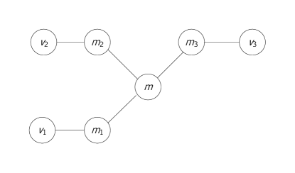
(a) Starlike tree

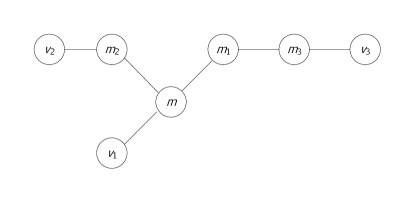
(b) Transformed tree

Figure 1: Transformation of stralike tree

Lemma 2

Given sequence of positive vertex weights $\mathbf{w}$ and degree sequence $\mathbf{d}$ of the same length, any optimal tree $T^{*}\in\mathcal{WT}(\mathbf{w},\mathbf{d})$ is a caterpillar.

Proof

All the trees with at most three internal vertices are caterpillars, so, without the loss of generality assume that there are at least four elements with $d_{i}>1$. Assume, by contradiction, that $T^{*}$ is not a caterpillar. Then an internal vertex $m\in M(T^{*})$ exists being adjacent to three other internal vertices (let us denote them with $m_{1},m_{2}$ $m_{3}$). Since vertex $m_{i}$ is internal, it has at least one more adjacent vertex distinct from $m$. Denote this adjacent vertex with $v_{i}$, $i=1,2,3$.

Deleting any vertex $v\in V(T^{*})$ and its incident edges in tree $T^{*}$, one obtains $d_{T^{*}}(v)$ connected components called induced subtrees. Let $\mu$ stand for the sum of weights of vertex $m$ and the vertices of all subtrees induced by deletion of $m$ from $T^{*}$ and containing neither of the vertices $m_{1},m_{2},m_{3}$. Similarly, let $\mu_{i}^{\prime}$, $i=1,2,3$, stand for the sum of weights of vertex $m_{i}$ and vertices of all subtrees induced by deleting $m_{i}$ from $T^{*}$ and containing neither $m$ nor $v_{i}$. Finally, let $\mu_{i}^{\prime\prime}$, $i=1,2,3$, stand for the sum of vertex weights in a subtree induced by deletion of vertex $m_{i}$ and containing vertex $v_{i}$.

Without loss of generality assume that $\mu_{1}^{\prime}+\mu_{1}^{\prime\prime}\leqslant\mu_{2}^{\prime}+\mu_{2}^{\prime\prime}\leqslant\mu_{3}^{\prime}+\mu_{3}^{\prime\prime}$. Let us consider a tree $T^{**}\in\mathcal{WT}(\mathbf{w},\mathbf{d})$ obtained from $T^{*}$ by replacing edges $mm_{3}$ and $m_{1}v_{1}$ with edges $mv_{1}$ and $m_{1}m_{3}$.

It is clear that $VWWI(T^{**})-VWWI(T^{*})=VWWI(T^{\prime})-VWWI(T)$, where $T$ and $T^{\prime}$ are the trees from the statement of Lemma 1. Since all vertex weights are assumed positive, from Lemma 1 it follows that $VWWI(T^{\prime})>VWWI(T)$ and $T^{*}$ cannot be optimal. The obtained contradiction completes the proof. _■

_□

Lemma 2 does not cover an important case of the terminal Wiener index. If zero weights are allowed, an optimal caterpillar still exists, though, similarly to the results by [44], not all optimal trees have to be caterpillars.

Corollary 1

If zero weights are allowed in Lemma 2, an optimal caterpillar exists.

Proof

Introduce the notation

$$VWWI^{*}:=\max\left\{VWWI(T):T\in\mathcal{WT}(\mathbf{w},\mathbf{d})\right\},$$

$$VWWI^{\prime}:=\max\left\{VWWI(T):T\in\mathcal{WT}(\mathbf{w},\mathbf{d}),VWWI(T)<VWWI^{*}\right\},$$

$$\delta:=VWWI^{*}-VWWI^{\prime}.$$

Since the set $\mathcal{WT}(\mathbf{w},\mathbf{d})$ is finite, $\delta>0$.

Select any positive $\alpha<\sqrt{\frac{2\delta}{n^{3}}}$ and consider weight sequence $\mathbf{w}^{\alpha}=(\mu^{\alpha}_{1},...,\mu^{\alpha}_{n})=(\mu_{1}+\alpha,...,\mu_{n}+\alpha)$. Let $T^{\alpha}$ be an arbitrary optimal tree over $\mathcal{WT}(\mathbf{w}^{\alpha},\mathbf{d})$. From Lemma 2, $T^{\alpha}$ is a caterpillar. Introduce caterpillar $T^{\alpha}_{0}\in\mathcal{WT}(\mathbf{w},\mathbf{d})$ obtained from $T^{\alpha}$ by decreasing all vertex weights by $\alpha$. It is clear that

$$VWWI^{*}\leqslant VWWI(T^{\alpha})=\\ VWWI(T^{\alpha}_{0})+\frac{\alpha^{2}}{2}\sum_{u,v\in V(T^{\alpha})}d_{T^{\alpha}}(u,v)\leqslant VWWI(T^{\alpha}_{0})+\frac{\alpha^{2}n^{3}}{2}.$$ (6)

Therefore, $VWWI(T^{\alpha}_{0})\geqslant VWWI^{*}-\frac{\alpha^{2}n^{3}}{2}>VWWI^{*}-\delta=VWWI^{\prime}$. Consequently, $VWWI(T^{\alpha}_{0})=VWWI^{*}$, and caterpillar $T^{\alpha}_{0}$ is optimal. _■

_□

5 Structure of Optimal Caterpillar

Definition 9

Numeric sequence $a_{1},...,a_{q}$ is called V-shaped if there exists such $\underline{k}\in\{1,...,q\}$, that $a_{k}\geqslant a_{k+1}$ for $k<\underline{k}$ and $a_{k}\leqslant a_{k+1}$ for $k\geqslant\underline{k}$. _□

Definition 10

Let us consider a (vertex-weighted) caterpillar $T\in\mathcal{WT}$ with backbone $v_{1},...,v_{q}$. Vertex $v\in V(T)$ is associated with backbone position $k\in\{1,...,q\}$, if either $v=v_{k}$ or $v\in W(T),vv_{k}\in E(T)$. Let $A_{T}(k)$ stand for the set of vertices associated with backbone position $k$ of caterpillar $T$ and their total weight is denoted with

$$w_{T}(k):=\sum_{v\in A_{T}(k)}\mu_{T}(v).$$ (7)

The value $p_{T}(k):=\sum_{l=1}^{q}w_{T}(l)|k-l|$, $k=1,...,q$, is called the price of $k$-th position on the backbone of caterpillar $T$. _□

It is shown in [10] that if caterpillar $T\in\mathcal{T}(\mathbf{d})$ with backbone $v_{1},...,v_{q}$ maximizes $WI$, then sequence $d_{T}(v_{k})$, $k=1,...,q$, is V-shaped. This result is extended below by proving that the sequences of pendent and internal vertex weights and the sequence of internal vertex degrees are V-shaped in some optimal caterpillar, and the same is true for any optimal caterpillar with positive vertex weights.

For any pair of pendent vertices $u_{k}\in A_{T}(k),v_{l}\in A_{T}(l)$ of vertex-weighted caterpillar $T$ $d_{T}(u,v)=2+|k-l|$; for pendent vertex $u\in A_{T}(k)$ and internal vertex $v\in A_{T}(l)$ $d_{T}(u,v)=1+|k-l|$. Therefore, the value of the Wiener index can be written as

$$VWWI(T)=\sum_{k=1}^{q}w_{T}(k)p_{T}(k)+\sum_{v\in V(T)}\mu_{T}(v)\sum_{v\in M(T)}\mu_{T}(v)-\sum_{v\in W(T)}\mu_{T}(v)^{2}.$$ (8)

Note that if a pair of caterpillars share the same weight and degree sequences, they differ only in the first term in (8).

Lemma 3

Let $\mathbf{w}$ be a positive weight sequence. Consider an optimal caterpillar $T\in\mathcal{WT}(\mathbf{w},\mathbf{d})$ and let $v_{1},...,v_{q}$ be its backbone. If $u_{k}\in A_{T}(k)$ is an arbitrary pendent vertex associated with $k$-th backbone position, then the sequence of pendent vertex weights $\mu_{T}(u_{k})$, $k=1,...,q$, is V-shaped.

Proof

Assume, by contradiction, that the sequence of pendent vertex weights is not V-shaped. Then $\mu_{T}(u_{k-1})<\mu_{T}(u_{k})>\mu_{T}(u_{k+1})$ for some $k\in\{2,...,q-1\}$. Let us consider caterpillar $T^{\prime}\in\mathcal{WT}(\mathbf{w},\mathbf{d})$ obtained from $T$ by replacing edges $u_{k}v_{k}$ and $u_{k-1}v_{k-1}$ with edges $u_{k}v_{k-1}$ and $u_{k-1}v_{k}$ and also caterpillar $T^{\prime\prime}\in\mathcal{WT}(\mathbf{w},\mathbf{d})$ obtained from $T$ by replacing edges $u_{k}v_{k}$ and $u_{k+1}v_{k+1}$ with edges $u_{k}v_{k+1}$ and $u_{k+1}v_{k}$. From Equation (8) it follows that

$$VWWI(T^{\prime})-VWWI(T)=\frac{1}{2}\left(\mu_{T}(u_{k})-\mu_{T}(u_{k-1})\right)\left(p_{T+T^{\prime}}(k-1)-p_{T+T^{\prime}}(k)\right),$$

$$VWWI(T^{\prime\prime})-VWWI(T)=\frac{1}{2}\left(\mu_{T}(u_{k})-\mu_{T}(u_{k+1})\right)\left(p_{T+T^{\prime\prime}}(k+1)-p_{T+T^{\prime\prime}}(k)\right),$$

where $p_{T+T^{\prime}}(k)$ is shorthand for $p_{T}(k)+p_{T^{\prime}}(k)$. Since $T$ is optimal, $VWWI(T^{\prime})\leqslant VWWI(T)\geqslant VWWI(T^{\prime\prime})$. By assumption, $\mu_{T}(u_{k-1})<\mu_{T}(u_{k})>\mu_{T}(u_{k+1})$, so

$$p_{T+T^{\prime}}(k-1)\leqslant p_{T+T^{\prime}}(k),p_{T+T^{\prime\prime}}(k+1)\leqslant p_{T+T^{\prime\prime}}(k)$$

and, therefore,

$$p_{T}(k-1)+p_{T^{\prime}}(k-1)+p_{T}(k+1)+p_{T^{\prime\prime}}(k+1)\leqslant 2p_{T}(k)+p_{T^{\prime}}(k)+p_{T^{\prime\prime}}(k).$$ (9)

On the other hand, by the definition of position prices,

$$p_{T^{\prime}}(k)-p_{T}(k)=p_{T}(k-1)-p_{T^{\prime}}(k-1)=\mu_{T}(u_{k})-\mu_{T}(u_{k-1}),$$

$$p_{T^{\prime\prime}}(k)-p_{T}(k)=p_{T}(k+1)-p_{T^{\prime\prime}}(k+1)=\mu_{T}(u_{k})-\mu_{T}(u_{k+1}).$$

Substituting into Expression (9) and dividing by two, we have

$$p_{T}(k-1)+p_{T}(k+1)\leqslant 2p_{T}(k)+\mu_{T}(u_{k})-\mu_{T}(u_{k-1})+\mu_{T}(u_{k})-\mu_{T}(u_{k+1}).$$

Taking into account that $p_{T}(k-1)+p_{T}(k+1)-2p_{T}(k)=2w_{T}(k)\geqslant 2\mu_{T}(u_{k})$, we finally obtain $\mu_{T}(u_{k-1})+\mu_{T}(u_{k+1})\leqslant 0$, which is impossible for positive vertex weights. The obtained contradiction completes the proof. _■

_□

Lemma 4

Assume positive weight sequence $\mathbf{w}$ is monotone in degrees $\mathbf{d}$. Then in optimal caterpillar $T\in\mathcal{WT}(\mathbf{w},\mathbf{d})$ with backbone $v_{1},...,v_{q}$, the sequence of internal vertex weights $\mu_{T}(v_{k})$ and the sequence of internal vertex degrees $d_{T}(v_{k})$, $k=1,...,q$, are V-shaped.

Proof

Assume that the sequence of internal vertex weights is not V-shaped. Then $\mu_{T}(v_{k-1})<\mu_{T}(v_{k})>\mu_{T}(v_{k+1})$ for some $k\in\{2,...,q-1\}$. Since weights are degree-monotone, we also conclude that $d_{T}(v_{k-1})\leqslant d_{T}(v_{k})\geqslant d_{T}(v_{k+1})$. Denote $d^{\prime}:=d_{T}(v_{k})-d_{T}(v_{k-1})\geqslant 0$ and $d^{\prime\prime}:=d_{T}(v_{k})-d_{T}(v_{k+1})\geqslant 0$.

Let us select $d^{\prime}$ arbitrary pendent vertices adjacent to vertex $v_{k}$ and denote their total weight with $\mu^{\prime}\geqslant 0$. Consider caterpillar $T^{\prime}$ obtained from $T$ by reconnecting all the other incident edges of vertex $v_{k}$ to vertex $v_{k-1}$ and reconnecting all the incident edges of vertex $v_{k-1}$ to vertex $v_{k}$. It is clear that $T^{\prime}\in\mathcal{WT}(\mathbf{w},\mathbf{d})$ and

$$VWWI(T^{\prime})-VWWI(T)=\frac{1}{2}(\mu^{\prime}+\mu_{T}(v_{k})-\mu_{T}(v_{k-1}))\left(p_{T+T^{\prime}}(k-1)-p_{T+T^{\prime}}(k)\right).$$

Caterpillar $T$ is optimal, so $VWWI(T^{\prime})\leqslant VWWI(T)$ and since, by assumption, $\mu_{T}(v_{k})>\mu_{T}(v_{k-1})$, $\mu^{\prime}\geqslant 0$, we conclude that $p_{T+T^{\prime}}(k-1)\leqslant p_{T+T^{\prime}}(k)$. In a similar manner it is shown that $p_{T+T^{\prime\prime}}(k+1)\leqslant p_{T+T^{\prime\prime}}(k)$ and, therefore,

$$p_{T}(k-1)+p_{T^{\prime}}(k-1)+p_{T}(k+1)+p_{T^{\prime\prime}}(k+1)\leqslant 2p_{T}(k)+p_{T^{\prime}}(k)+p_{T^{\prime\prime}}(k).$$ (10)

Similarly to Lemma 3, we write

$$p_{T^{\prime}}(k)-p_{T}(k)=p_{T}(k-1)-p_{T^{\prime}}(k-1)=\mu_{T}(v_{k})-\mu_{T}(v_{k-1})+\mu^{\prime},$$

$$p_{T^{\prime\prime}}(k)-p_{T}(k)=p_{T}(k+1)-p_{T^{\prime\prime}}(k+1)=\mu_{T}(v_{k})-\mu_{T}(v_{k+1})+\mu^{\prime},$$

$$p_{T}(k-1)+p_{T}(k+1)-2p_{T}(k)=2w_{T}(k)\geqslant 2(\mu_{T}(v_{k})+\mu^{\prime})>0,$$

so inequality (10) reduces to $\mu_{T}(v_{k-1})+\mu_{T}(v_{k+1})\leqslant 0$, which is impossible for positive weights. The obtained contradiction proves that the sequence of internal vertex weights is V-shaped. The same argument can be used to show that the sequence of internal vertex degrees is, indeed, V-shaped. _■

_□

Corollary 2

If zero vertex weights are allowed in Lemmas 3 and 4, then optimal caterpillar $T\in\mathcal{WT}(\mathbf{w},\mathbf{d})$ with backbone $v_{1},...,v_{q}$ exists, where the following sequences are V-shaped for $k=1,...,q$: internal vertex weights $\mu_{T}(v_{k})$, internal vertex degrees $d_{T}(v_{k})$, and pendent vertex weights $\mu_{T}(u_{k})$ for any $u_{k}\in A_{T}(k)$. _□

The proof is similar to that of Corollary 1.

6 Upper-Bound Estimate

Let us consider non-negative weight sequence $\mathbf{w}=(\mu_{1},...,\mu_{n})$ and natural degree sequence $\mathbf{d}=(d_{1},...,d_{n})$, $d_{i}>1$, $i=1,...,q$, $d_{i}=1$, $i=q+1,...,n$, $q\geqslant 4$. As before, sequence $\mathbf{d}$ is non-increasing, and elements in $\mathbf{w}$ that share the same degree in $\mathbf{d}$, go in the decreasing order of their weights. In this section it is shown that if weight sequence $\mathbf{w}$ is monotone in degrees $\mathbf{d}$, then, for any $T\in\mathcal{WT}(\mathbf{w},\mathbf{d})$ inequality $VWWI(T)\leqslant UB(\mathbf{w},\mathbf{d})$ holds, where

$$UB(\mathbf{w},\mathbf{d})=\mu\left[\frac{q+1}{4}\mu+\sum_{i=1}^{q}\mu_{i}\right]-\sum_{i=q+1}^{n}\mu_{i}^{2}-\sum_{k=1}^{\lceil\frac{q}{2}\rceil}2M_{k}\left[kM_{k}+2\sum_{l=1}^{k-1}lM_{l}\right],$$ (11)

$\mu:=\sum_{i=1}^{n}\mu_{i}$, $M_{k}:=\frac{1}{2}\left(\mu_{2k-1}+\mu_{2k}+\sum_{i=1+D_{k-1}}^{D_{k}}\mu_{q+i}\right)$ for $k=1,...,\lfloor\frac{q}{2}\rfloor$, $M_{\lfloor\frac{q}{2}\rfloor+1}:=\frac{1}{2}\left(\mu_{q}+\sum_{i=0}^{d_{q}-3}\mu_{n-i}\right)$, $D_{0}:=0$, $D_{1}:=d_{1}+d_{2}-2$, $D_{k}=2+\sum_{i=1}^{2k}(d_{i}-2)$ for $k=2,...,\lceil\frac{q}{2}\rceil$.

According to expression (8), the optimal caterpillar problem (OCP) reduces to the assignment of internal and pendent vertices to positions on the caterpillar’s backbone taking into account vertex degree constraints. Let $T\in\mathcal{WT}(\mathbf{w},\mathbf{d})$ be a caterpillar with vertices $v_{1},...,v_{n}$ indexed so as $\mu_{T}(v_{i})=\mu_{i},d_{T}(v_{i})=d_{i}$, and let $X$ be the assignment matrix, i.e., $x_{ik}=1$ when vertex $v_{i}$, $i=1,...,n$, is associated with backbone position $k=1,...,q$, i.e., $v_{i}\in A_{T}(k)$, otherwise $x_{ik}=0$. Then the weight associated with backbone position $k=1,...,q$ of caterpillar $T$ is written as

$$w_{k}(X|\mathbf{w},\mathbf{d})=\sum_{i=1}^{n}\mu_{i}x_{ik},k=1,...,q,$$ (12)

and position prices are written as

$$p_{k}(X|\mathbf{w},\mathbf{d})=\sum_{l=1}^{q}w_{l}(X|\mathbf{w},\mathbf{d})|k-l|=\sum_{i=1}^{n}\mu_{i}\sum_{l=1}^{q}x_{il}|k-l|,k=1,...,q.$$ (13)

Taking into account expressions (8) and (13), the Wiener index of tree $T$ is written using matrix $X$ as

$$VWWI(X|\mathbf{w})=\frac{1}{2}\sum_{i,j=1}^{n}\sum_{k,l=1}^{q}\mu_{i}x_{ik}\mu_{j}x_{jl}|k-l|+\sum_{i=1}^{n}\mu_{i}\sum_{j=1}^{q}\mu_{j}-\sum_{i=q+1}^{n}\mu_{i}^{2},$$ (14)

To simplify notation let us skip $\mathbf{w}$ and $\mathbf{d}$ when it does not lead to confusion.

Only the first term depends on assignment matrix $X$, so OCP reduces to the following binary quadratic program:

Maximize $$\frac{1}{2}\sum_{i,j=1}^{n}\sum_{k,l=1}^{q}\mu_{i}x_{ik}\mu_{j}x_{jl}|k-l|$$ (15)

subject to constraints:

discreteness: $$x_{ik}\in\{0,1\},i=1,...,n,k=1,...,q,$$ (16)

unique assignment: $$\sum_{k=1}^{q}x_{ik}=1,i=1,...,n,$$ (17)

internal vertex assignment: $$\sum_{i=1}^{q}x_{ik}=1,k=1,...,q,$$ (18)

balance of vertex degrees: $$\sum_{i=1}^{n}(d_{i}-2)x_{ik}=0,k=2,...,q-1,$$ (19)

$$\sum_{i=1}^{n}(d_{i}-2)x_{ik}=-1,k=1,q.$$ (20)

This problem is similar to the Wiener-type QAP introduced in [10], and is NP-complete, since it is a generalization of the classic partition problem (Setting $q=2$, $n=2+2k$, $\mu_{1}=\mu_{2}=0$, $d_{1}=d_{2}=k$ makes a partition problem for $2k$ elements.)

The continuous relaxation of problem (15) is obtained by replacing discreteness constraints (16) with box constraints

$$x_{ik}\in[0,1].$$ (21)

The function in expression (15) is concave on the feasible set: to verify, use condition (17) and obtain an equivalent problem

$$\frac{1}{2}\sum_{i,j=1}^{n}\sum_{k,l=1}^{q}\mu_{i}x_{ik}\mu_{j}x_{jl}|k-l|=\frac{q-1}{2}\left(\mu_{1}+...+\mu_{n}\right)^{2}-\frac{1}{2}\min_{X}\mathbf{w}^{\textrm{T}}XPX^{\textrm{T}}\mathbf{w},$$

where matrix $P:=(q-1-|k-l|)_{k,l=1}^{q}$ is positive semidefinite, since it can be written as the following sum of positively definite rank-one matrices

$$P=\sum_{i=1}^{q-1}\left[(\underbrace{1,...,1}_{i\text{ times}},\underbrace{0,...,0}_{q-i\text{ times}})^{\mathrm{T}}\cdot(\underbrace{1,...,1}_{i\text{ times}},\underbrace{0,...,0}_{q-i\text{ times}})+\right.\\ \left.+(\underbrace{0,...,0}_{i\text{ times}},\underbrace{1,...,1}_{q-i\text{ times}})^{\mathrm{T}}\cdot(\underbrace{0,...,0}_{i\text{ times}},\underbrace{1,...,1}_{q-i\text{ times}})\right].$$ (22)

Therefore, the relaxed OCP (ROCP) (15) with constraints (17)-(21) is a convex quadratic program with linear constraints.

It is clear from (15) that OCP and ROCP do not change if one reverses the numbering of caterpillar backbone positions. Therefore, if matrix $X$ is an optimal solution of ROCP, then matrix $X^{\prime}$ obtained from $X$ by applying inverse column order is also optimal. Matrix $X^{\prime\prime}=\frac{X+X^{\prime}}{2}$ is a feasible ROCP solution and, since the optimization criterion is concave, $X^{\prime\prime}$ is also optimal. Therefore, when studying ROCP, we can limit ourselves to symmetric solutions, where $x_{ik}=x_{i,q-k+1}$. Prices $p_{k}(X)$ are also symmetric with respect to the central backbone position.

Similar to Lemma 3, in the optimal ROCP solution vertices with bigger weights are associated with outermost backbone positions. Lemma 5 concerns pendent vertices, while Lemma 6 is about internal vertices.

Lemma 5

Let $\mathbf{w}$ be a weight sequence with pairwise distinct elements, and let $X$ be an optimal symmetric solution of ROCP for weight sequence $\mathbf{w}$ and degree sequence $\mathbf{d}$. If $x_{i,k-1}>0$ and $x_{jk}>0$ for some $i,j\in\{q+1,...,n\}$ and $k\leqslant\lceil\frac{q}{2}\rceil$, then $i\leqslant j$.

Proof

The proof is similar to that of Lemma 3. Let us assume, by contradiction, that $i>j$ (and hence, $\mu_{j}>\mu_{i}$, as weights are pairwise distinct). Let us consider $n\times q$-matrix $\Delta$ with $\Delta_{j,k-1}=\Delta_{ik}=-\Delta_{jk}=-\Delta_{i,k-1}=\delta>0$ and all other elements being zeros. Assume that $\delta<\min\left(x_{i,k-1},x_{jk}\right)$, so $X+\Delta$ is a feasible ROCP solution. Since $X$ is optimal,

$$VWWI(X+\Delta)-VWWI(X)=\delta\left(\mu_{j}-\mu_{i}\right)\left(p_{k-1}(X)-p_{k}(X)-\delta(\mu_{j}-\mu_{i})\right)\leqslant 0.$$ (23)

By assumption, $\mu_{j}-\mu_{i}>0$ and $\delta>0$. Hence, $p_{k-1}(X)-p_{k}(X)-\delta(\mu_{j}-\mu_{i})\leqslant 0$, which is equivalent to $R-L+w_{k}(X)-\delta(\mu_{j}-\mu_{i})\leqslant 0$, where $L:=\sum_{l=1}^{k-1}w_{l}(X)$, $R:=\sum_{l=k+1}^{q}w_{l}(X)$. Since $X$ is a symmetric solution and $k\leqslant\lceil\frac{q}{2}\rceil$, inequality $R\geqslant L$ always holds and, consequently, $w_{k}(X)-\delta(w_{j}-w_{i})\leqslant 0$. On the other hand, from $\delta<x_{jk}$ it follows that $w_{k}(X)\geqslant x_{jk}\mu_{j}>\mu_{j}\delta$, so we obtain $\delta\mu_{i}<0$, which is impossible. The obtained contradiction proves the lemma. _■

_□

Lemma 6

Assume weight sequence $\mathbf{w}$, consisting of pairwise distinct elements, is monotone with respect to degree sequence $\mathbf{d}$. Let $X$ be an optimal symmetric ROCP solution for weight sequence $\mathbf{w}$ and degree sequence $\mathbf{d}$. If $x_{i,k-1}>0$ and $x_{jk}>0$ for some $i,j\in\{1,...,q\}$ and $k\leqslant\lceil\frac{q}{2}\rceil$, then $i\leqslant j$.

Proof

The proof is similar to that of Lemma 4. Assume, by contradiction, that $j<i$. Since weights are pairwise distinct, it follows that $\mu_{j}>\mu_{i}$, and since weights are degree-monotone, it follows that $d_{j}\geqslant d_{i}$. Let us denote $d:=d_{j}-d_{i}\geqslant 0$ and consider $n\times q$-matrix $\Delta$ with $\Delta_{j,k-1}=\Delta_{ik}=-\Delta_{jk}=-\Delta_{i,k-1}=\delta>0$, $\Delta_{v,k-1}=-\Delta_{vk}=\delta dx_{vk}(\sum_{v=1}^{n}x_{vk})^{-1},v=q+1,...,n$, and all other elements being zeros; also introduce the shorthand $\mu:=\delta d\sum_{v=q+1}^{n}\mu_{v}x_{vk}\left(\sum_{v=q+1}^{n}x_{vk}\right)^{-1}$.

Let us choose $\delta$ so as $\delta<\min\left(x_{i,k-1},x_{jk},\right)$ and $d\delta<\sum_{v=q+1}^{n}x_{vk}$. Matrix $X+\Delta$ is a feasible ROCP solution, so

$$VWWI(X+\Delta)-VWWI(X)=\\ \delta\left(\mu+\mu_{j}-\mu_{i}\right)\left(p_{k-1}(X)-p_{k}(X)-\delta(\mu+\mu_{j}-\mu_{i})\right).$$ (24)

The rest of the proof repeats that of Lemma 5. _■

_□

Lemmas 5 and 6 are refined by the following corollaries.

Corollary 3

Under the conditions of Lemma 6, if $x_{ik}>0$ for some $i\in\{1,...,q\}$ and $k\leqslant\lceil\frac{q}{2}\rceil$, then $x_{jl}=0$ for all $j=1,...,i$, $l=k+1,...,\lceil\frac{q}{2}\rceil$.

Proof

The proof is by contradiction. Firstly, let us assume that $x_{jl}>0$ for some $j\in\{1,...,i-1\}$, $l\in\{k+1,...,\lceil\frac{q}{2}\rceil\}$. From condition (18), for every $k^{\prime}\in\{k,...,l\}$ we have $x_{i^{\prime}k^{\prime}}>0$ for some $i^{\prime}\in\{1,...,q\}$. But by Lemma 6, if $x_{i^{\prime}k^{\prime}}>0$ then $x_{i^{\prime\prime},k^{\prime}+1}=0$ for all $i^{\prime\prime}=1,...,i^{\prime}-1$, so $x_{jl}>0$ is impossible for $1\leqslant j<i$.

Secondly, let us assume that $x_{ik},x_{il}>0$ for some $i\in\{1,...,q\}$, $k,l\leqslant\lceil\frac{q}{2}\rceil$. Without loss of generality assume that $k<l$ and $x_{jk}=0$ for all $j=1,...,i-1$. From condition (17) it follows that $x_{ik}+x_{il}\leqslant 1$, so $x_{ik}\leqslant 1-x_{il}<1$. Then, from condition (20), there exists such $j>i$ that $x_{jk}>0$. But it is shown above that $x_{jk}>0,x_{il}>0$ is impossible. The obtained contradiction completes the proof. _■

_□

Corollary 4

If equal weights are allowed for weight sequence $\mathbf{w}$ in Lemma 6, then such a symmetric ROCP solution $X$ exists that $x_{ik}>0$ for some $i\in\{1,...,q\}$ and $k\in\{1,...,\lceil\frac{q}{2}\rceil\}$ implies that $x_{jl}=0$ for all $j=1,...,i$, $l=k+1,...,\lceil\frac{q}{2}\rceil$.

Proof

Let $\varepsilon:=\min_{i,j:\mu_{i}>\mu_{j}}\left(\mu_{i}-\mu_{j}\right)$ be the minimum positive pairwise weight difference of the elements of sequence $\mathbf{w}$. Select any positive $\alpha<\varepsilon$ and consider sequence $\mathbf{w}^{\alpha}=(\mu^{\alpha}_{i})_{i=1}^{n}=(\mu_{i}+\alpha/i)_{i=1}^{n}$ of pairwise distinct positive weights. Let $X^{\alpha}$ be any optimal ROCP solution for weight sequence $\mathbf{w}^{\alpha}$ and degree sequence $\mathbf{d}$. The feasible set of ROCP does not depend on weights, so $X^{\alpha}$ is also feasible in ROCP for weight sequence $\mathbf{w}$.

Let us consider an infinite sequence $X^{\frac{\varepsilon}{t+1}}$, $t=1,2,...$. Its elements belong to the bounded compact set, so, without loss of generality, it converges (say, in Manhattan metric) to some feasible solution $X^{*}=(x_{ik}^{*})$. It is clear that $VWWI(X^{\alpha}|\mathbf{w})\leqslant VWWI^{*}\leqslant VWWI(X^{\alpha}|\mathbf{w}^{\alpha})\leqslant VWWI(X^{\alpha}|\mathbf{w})+\alpha n^{3}$ for any positive $\alpha$, where $VWWI^{*}$ is the optimal value of ROCP. Therefore, $VWWI(X^{*})=VWWI^{*}$ and $X^{*}$ is optimal.

Assume, by contradiction, that such $i,j\in\{1,...,q\}$ and $k,l\leqslant\lceil\frac{q}{2}\rceil$, $j\leqslant i$, $k<l$, exist that $x_{ik}^{*}>0$,$x_{jl}^{*}>0$, and $i>j$. By Corollary 3, for any $t=1,2,...$, and $\alpha=\frac{\varepsilon}{t+1}$ either $x_{i,k}^{\alpha}=0$ or $x_{jl}^{\alpha}=0$, so Manhattan distance between $X^{\alpha}$ and $X^{*}$ is at least $\min[x_{ik}^{*},x_{jl}^{*}]$ and sequence $X^{\frac{\varepsilon}{t+1}}$ cannot converge to $X^{*}$. The obtained contradiction completes the proof. _■

_□

Corollary 5

Under the conditions of Lemma 5, if $x_{ik}>0$ for some $i\in\{q+1,...,n\}$ and $k\leqslant\lceil\frac{q}{2}\rceil$, then $x_{jl}=0$ for all $j=q+1,...,i$, $l=k+1,...,\lceil\frac{q}{2}\rceil$. _□

The proof is similar to that of Corollary 3.

Corollary 6

If equal weights are allowed in weight sequence $\mathbf{w}$ in Lemma 5, then such symmetric solution $X$ of ROCP exists that $x_{ik}>0$ for some $i\in\{q+1,...,n\}$ and $k\in\{1,...,\frac{q}{2}\rceil\}$ implies that $x_{jl}=0$ for all $j=q+1,...,i$, $l=k+1,...,\lceil\frac{q}{2}\rceil$. _□

The proof is similar to that of Corollary 4.

Theorem 1

For odd $q$ the “double V-shaped” matrix

$$\small X=\begin{array}[]{cc}\begin{array}[]{ccccccc}&&&\lceil\frac{q}{2}\rceil&&&\\ \end{array}&\\ \left(\begin{array}[]{ccccccccc}0.5&0&...&&&&...&0&0.5\\ 0.5&0&...&&&&...&0&0.5\\ 0&0.5&...&&&&...&0.5&0\\ 0&0.5&...&&&&...&0.5&0\\ ...&...&...&...&...&...&...&...&...\\ 0&0&...&0.5&0&0.5&...&0&0\\ 0&0&...&0.5&0&0.5&...&0&0\\ 0&0&...&0&1&0&...&0&0\\ 0.5&0&...&&&&...&0&0.5\\ ...&...&...&&&&...&...&..\\ 0.5&0&0&&&&...&0&0.5\\ 0&0.5&0&...&&...&0&0.5&0\\ ...&...&...&&&&...&...&...\\ 0&0.5&0&...&&...&0&0.5&0\\ ...&...&...&...&...&...&...&...&...\\ 0&...&0&0.5&0&0.5&0&...&0\\ ...&...&...&...&...&...&...&...&...\\ 0&...&0&0.5&0&0.5&0&...&0\\ 0&0&...&0&1&0&...&0&0\\ ...&...&...&...&...&...&&...&...\\ 0&...&...&0&1&0&...&...&0\end{array}\right)&\begin{array}[]{l}\left.\begin{array}[]{c}\\ \\ \end{array}\right\}2\text{ times}\\ \left.\begin{array}[]{c}\\ \\ \end{array}\right\}2\text{ times}\\ \\ \left.\begin{array}[]{c}\\ \\ \end{array}\right\}2\text{ times}\\ \\ \left.\begin{array}[]{c}\\ \\ \\ \end{array}\right\}d_{1}+d_{2}-2\text{ times}\\ \left.\begin{array}[]{c}\\ \\ \\ \end{array}\right\}d_{3}+d_{4}-4\text{ times}\\ \\ \left.\begin{array}[]{c}\\ \\ \\ \end{array}\right\}d_{q-2}+d_{q-3}-4\text{ times}\\ \left.\begin{array}[]{c}\\ \\ \\ \end{array}\right\}d_{q}-2\text{ times}\end{array}\end{array}\normalsize$$ (25)

is a solution of ROCP. In case of even $q$ the “central” column (the one marked with $\lceil\frac{q}{2}\rceil$) is missing in (25).

Proof

Let us consider the case of odd $q$. From Corollaries 4 and 6 it follows that a symmetric ROCP soluton $X$ exists where the first $\lceil\frac{q}{2}\rceil$ columns have a single non-zero element in each row. From the symmetry of solution $X$ and condition (17), non-zero element $x_{ik}=\frac{1}{2}$ for $k<\lceil\frac{q}{2}\rceil$ and $x_{i\lceil\frac{q}{2}\rceil}=1$. Corollary 4 says that non-zero elements for the first $q$ rows and first $\lceil\frac{q}{2}\rceil$ columns go from the top-left corner to the bottom-right, and from condition (18) it follows that column $\lceil\frac{q}{2}\rceil$ has a single non-zero element, while all the other columns have exactly two non-zero elements in the first $q$ rows.

The placement of non-zero elements for rows from $q+1$ to $n$ is justified in the same manner, with the only difference that the number of non-zero elements in each column is determined by condition (20). The case of even $q$ is considered similarly, except that column $\lceil\frac{q}{2}\rceil$ does not play any special role. _■

_□

Corollary 7

If weight sequence $\mathbf{w}$ is monotone in degree sequence $\mathbf{d}$, expression (11) gives an upper bound of the Wiener index over $\mathcal{WT}(\mathbf{w},\mathbf{d})$.

Proof

Expression (11) is obtained from expressions (14) and (25) with a series of simplifications that employ symmetry of function (15) and of solution $X$. Expression (14) gives an upper bound of the Wiener index for optimal caterpillar since matrix $X$ is a solution of a continuous relaxation of OCP. _■

_□

7 Quality of Upper Bound

Let us show first that upper bound (11) is tight.

Theorem 2

If in weight sequence $\mathbf{w}$ being monotone in degree sequence $\mathbf{d}$ we have $\mu_{2i-1}=\mu_{2i}$, $d_{2i-1}=d_{2i}$ for $i=1,...,\lfloor\frac{q}{2}\rfloor$ and $\mu_{q+2i-1}=\mu_{q+2i}$ for $i=1,...,\lfloor\frac{n-q}{2}\rfloor$ (i.e., the number of vertices with distinct degree and weight is even, while the pendent/internal vertex with the smallest weight may be unpaired in case of the odd number of pendent/internal vertices), then $UB(\mathbf{w},\mathbf{d})=VWWI(T)$ for some $T\in\mathcal{WT}(\mathbf{w},\mathbf{d})$.

Proof

Let $X=(x_{ik})$ be a ROCP solution defined by expression (25) and consider $X^{\prime}=(x_{ik}^{\prime})$, where for all $i=1,...,n$ and $k=1,...,q$

$$x_{ik}^{\prime}=\left\{\begin{array}[]{ll}1,&\hbox{$x_{ik}>0,i\leqslant q,k\leqslant\lceil{q/2}\rceil\text{ and }i\text{ is odd}$;}\\ 1,&\hbox{$x_{ik}>0,i\leqslant q,k\geqslant\lceil{q/2}\rceil\text{ and }i\text{ is even}$;}\\ 1,&\hbox{$x_{ik}>0,i>q,k\leqslant\lceil{q/2}\rceil\text{ and }i-q\text{ is odd}$;}\\ 1,&\hbox{$x_{ik}>0,i>q,k\geqslant\lceil{q/2}\rceil\text{ and }i-q\text{ is even}$;}\\ 0,&\hbox{otherwise,}\\ \end{array}\right.$$

i.e., in every pair of vertices with the same weight and degree distributed in $X$ equally between positions $k$ and $q-k+1$ of the caterpillar backbone, one is assigned to position $k$, and the other is assigned to position $q-k+1$. It is clear that $X^{\prime}$ is a feasible OCP solution, and $UB(\mathbf{w},\mathbf{d})=VWWI(X)=VWWI(X^{\prime})$, which completes the proof. _■

_□

From the proof of Theorem 2 it follows that for odd $q$ its conditions could be a bit weakened: $d_{q}-2$ pendent vertices with the smallest weight may be unpaired.

Let $T^{*}(\mathbf{w},\mathbf{d})$ be an optimal caterpillar for weight sequence $\mathbf{w}$ and degree sequence $\mathbf{d}$. The relative error of upper bound (11) is defined as

$$RE(\mathbf{w},\mathbf{d}):=\frac{UB(\mathbf{w},\mathbf{d})}{VWWI(T^{*}(\mathbf{w},\mathbf{d}))}-1.$$ (26)

Unfortunately, $RE(\mathbf{w},\mathbf{d})$ can be arbitrary high. For example, if $\mu_{1}>0$ and $\mu_{i}=0$ for $i>1$, then $VWWI(T)=0$ for every $T\in\mathcal{WT}(\mathbf{w},\mathbf{d})$, but $UB(\mathbf{w},\mathbf{d})>0$, so $\frac{UB(\mathbf{w},\mathbf{d})}{VWWI(T^{*}(\mathbf{w},\mathbf{d}))}$ is unbounded. Nevertheless, it is shown below that the average relative error is low enough, especially for large trees. Let us define

$$\delta_{k}=\left\{\begin{array}[]{ll}$1$,&\hbox{$k\in\{1,q\}$;}\\ $2$,&\hbox{otherwise.}\\ \end{array}\right.$$

The greedy heuristics shown in Listing 1 constructs a (nearly optimal) caterpillar for weight sequence $\mathbf{w}$ and degree sequence $\mathbf{d}$ by sequentially assigning vertices to the caterpillar backbone position with the maximum current price. Prices are re-calculated after each iteration, so two consequent vertices are typically spread as far as possible.

Listing 1 Greedy heuristic algorithm builds an approximately optimal caterpillar for weight sequence $\mathbf{w}$ and degree sequence $\mathbf{d}$

1:function GreedyCaterpillar($\mathbf{w}$, $\mathbf{d}$)

2:     $X\leftarrow 0_{n\times q}$ $\triangleright$ Start from the empty assignment table

3:     $X(q+1,1)\leftarrow 1$ $\triangleright$ Assign $1^{st}$ pendent vertex to the outermost backbone position

4:     $i\leftarrow 1$ $\triangleright$ Internal vertex counter

5:     $j=q+2$ $\triangleright$ Pendent vertex counter

6:     while $i<q$ or $j<n$ do $\triangleright$ Loop until unassigned vertices exist

7:         $k\leftarrow\operatorname*{arg\,max}\{p_{k^{\prime}}(X)|k^{\prime}:\sum_{i^{\prime}=1}^{q}x_{i^{\prime}k^{\prime}}<1\}$

8:         $l\leftarrow\operatorname*{arg\,max}\{p_{l^{\prime}}(X)|l^{\prime}:\sum_{j^{\prime}=q+1}^{n}x_{j^{\prime}l^{\prime}}<\sum_{i^{\prime}=1}^{q}d_{i^{\prime}}x_{i^{\prime}l^{\prime}}-\delta_{l^{\prime}}\}$

9:         if $\mu_{i}p_{k}(X)>\mu_{j}p_{l}(X)$ then

10:              $x_{ik}\leftarrow 1$ , $i\leftarrow i+1$

11:         else

12:              $x_{jl}\leftarrow 1$, $j\leftarrow j+1$

13:         end if

14:     end while

15:     return $X$

16:end function

The relative error can be estimated from above as

$$RE(\mathbf{w},\mathbf{d})\leqslant\widetilde{RE}(\mathbf{w},\mathbf{d})=\frac{UB(\mathbf{w},\mathbf{d})}{VWWI(\text{{GreedyCaterpillar}}(\mathbf{w},\mathbf{d})|\mathbf{w})}-1.$$

In Figure 2 the value of $\widetilde{RE}(\cdot)$ is presented as a function of the graph order. The minimum error is zero and the maximum tends to infinity, but these are extremely rare events. Therefore, the median (the bold line), the upper and the lower decile values (two thin lines) are shown in Figure 2 for 1000 randomly generated weight and degree sequences for each vertex count $n=6,...,100$. The median error never exceeds $1\%$, and even for relatively small trees (those with $n>12$ vertices) nine of ten graphs have error less than $1\%$. For moderately sized trees ($n>50$) the median relative error is less than $0.01\%$, and for $90\%$ of trees the relative error does not exceed $0.2\%$.

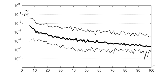
Figure 2: Estimated relative error of upper bound (11) vs graph order (logarithmic scale for the vertical axis)

8 Branch and Bound Scheme

Although it is shown in the previous section that both upper bound (11) and heuristic algorithm GreedyCaterpillar have good average quality, the question of the exact solution of OCP is still open. Since OCP reduces to the convex binary quadratic minimization program (15) with linear constraints (16)-(20), the branch and bound algorithms implemented in commercial solvers (like CPLEX) can be used to find an optimal caterpillar. Nevertheless, due to the large search space ($2^{n\times q}$ elements), they show low performance being inapplicable even for trees with a dozen of vertices.

In case of weights being monotone in degrees the search space can be decreased dramatically taking into account the characterization of the structure of an optimal caterpillar presented in Section 5. Let us restrict attention to optimal caterpillars with V-shaped weight sequences as stated by Corollary 2. Then it is clear, that one obtains any V-shaped assignment of internal vertices to positions on the caterpillar backbone by sequentially running through internal vertices in the order of descending weights and deciding whether to assign the vertex to the rightmost or to the leftmost vacant backbone position. Each decision is binary (right or left), so $2^{q}$ alternative assignments are to be considered.

In the same manner, with positions of internal vertices being fixed, any V-shaped assignment of pendent vertices is obtained by sequentially assigning pendent vertices to the rightmost or to the leftmost vacant backbone position taking care about vertex degree constraints. Therefore, the total search space has $2^{n}$ alternative assignments, which makes great economy.

The branch and bound algorithm presented in Listing 2 can be used to solve OCP for trees of moderate order ($n\approx 30$) on a PC. It systematically explores the search space by recursively assigning internal and pendent vertices to backbone positions as explained above (the branching takes place on whether the vertex is assigned to the left or to the right). If the best known solution outperforms the upper bound of $VWWI$ given the current partially fixed solution, then further branching is not required (enumeration is bounded).

GreedyCaterpillar($\mathbf{w},\mathbf{d}$) is used as a starting best known solution. The upper bound $UB(\mathbf{w},\mathbf{d}|X_{0})$ given partial assignment matrix $X^{0}=(x_{ik}^{0})$ is calculated as a solution of ROCP (15), (17)-(21) with additional box constraints $x_{ik}=1$ for such $i$ and $k$ that $x_{ik}^{0}=1$. This convex quadratic program is solved efficiently by many open-source and commercial packages. To improve performance, in our Matlab implementation branching on the next pendent vertex occurs immediately as a pair of vacant left and right positions appears on the caterpillar backbone, and the order of recursion (right then left or vice versa) is driven by the current price $p_{k}(X_{0})$ of backbone position, as in Listing 1.

Listing 2 Branch and bound algorithm for OCP

1:function OptimalCaterpillar($\mathbf{w}$, $\mathbf{d}$)

2:     $X_{0}\leftarrow 0_{n\times q}$ $\triangleright$ Start from empty assignment table

3:     $Best\leftarrow$ GreedyCaterpillar($\mathbf{w},\mathbf{d}$) $\triangleright$ The best known solution

4:     Branching($X_{0}$) $\triangleright$ Recursive solution branching

5:     Return $Best$ $\triangleright$ Branching leaves the solution in $Best$

6:end function

7:function Branching($X_{0}$) $\triangleright$ Recursive branching starting from partial solution $X_{0}$

8:     $i\leftarrow\min\{j:\sum_{l=1}^{q}x_{jl}^{0}=0\}$ $\triangleright$ $1^{st}$ unassigned vertex in $X_{0}$

9:     if $i<q$ then $\triangleright$ If unassigned internal vertex exists

10:         $k\leftarrow\max\{l:\sum_{j=1}^{q}x_{jl}^{0}=0\}$, $X_{R}\leftarrow X_{0}$, $x_{ik}^{R}\leftarrow 1$ $\triangleright$ Assign internal right

11:         if $VWWI$($UB(\mathbf{w},\mathbf{d}|X_{R})$)$>VWWI(Best)$ then

12:              Branching($X_{R}$)

13:         end if

14:         $k\leftarrow\min\{l:\sum_{j=1}^{q}x_{jl}^{0}=0\}$, $X_{L}\leftarrow X_{0}$, $x_{ik}^{L}\leftarrow 1$ $\triangleright$ Assign internal left

15:         if $VWWI$($UB(\mathbf{w},\mathbf{d}|X_{L})$)$>VWWI(Best)$ then

16:              Branching($X_{L}$)

17:         end if

18:     else if $i\leqslant n$ then $\triangleright$ If unassigned pendent vertices exist

19:         $k\leftarrow\max\{l:\sum_{j=q+1}^{n}x_{jl}^{0}<\sum_{j=1}^{q}d_{j}x_{jl}^{0}-\delta_{l}\}$, $X_{R}\leftarrow X_{0}$, $x_{ik}^{R}\leftarrow 1$ $\triangleright$ Assign right

20:         if $VWWI$($UB(\mathbf{w},\mathbf{d}|X_{R})$)$>VWWI(Best)$ then

21:              Branching($X_{R}$)

22:         end if

23:         $k\leftarrow\min\{l:\sum_{j=q+1}^{n}x_{jl}^{0}<\sum_{j=1}^{q}d_{j}x_{jl}^{0}-\delta_{l}\}$, $X_{L}\leftarrow X_{0}$, $x_{ik}^{L}\leftarrow 1$ $\triangleright$ Assign left

24:         if $VWWI$($UB(\mathbf{w},\mathbf{d}|X_{L})$)$>VWWI(Best)$ then

25:              Branching($X_{L}$)

26:         end if

27:     else if $VWWI(X_{0})>VWWI(Best)$ then $Best\leftarrow X_{0}$ $\triangleright$ Update the best

28:     end if

29:end function

To evaluate the performance of the algorithm, 100 random weight and degree sequences were generated for every graph order $n=6,...,30$. In Figure 3 the average computation time is shown as a function of $n$. It grows exponentially, which is expectable for the NP-complete problem.

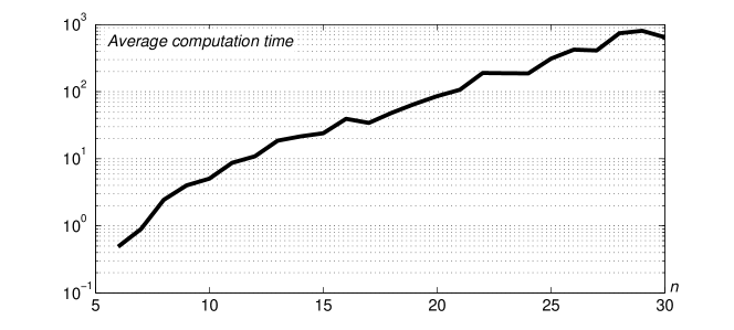
Figure 3: Average computation time of the branch and bound algorithm vs graph order (logarithmic scale for the vertical axis)

In Figure 4 upper bound (11) and the value of the Wiener index for GreedyCaterpillar are compared with the optimal Wiener index value. The thick solid line in Figure 4 is $RE(\mathbf{w},\mathbf{d})+1=\frac{UB(\mathbf{w},\mathbf{d})}{VWWI(T^{*}(\mathbf{w},\mathbf{d}))}$ averaged over 100 random weight and degree sequences for the given graph order $n$, while the dashed line is $\frac{VWWI(\text{{GreedyCaterpillar}}(\mathbf{w},\mathbf{d}))}{VWWI(T^{*}(\mathbf{w},\mathbf{d}))}$, also averaged. It can be seen that, although the gap between the index value for the greedy tree and the upper bound is typically small, filling this small gap by the branch and bound algorithm may take much time.

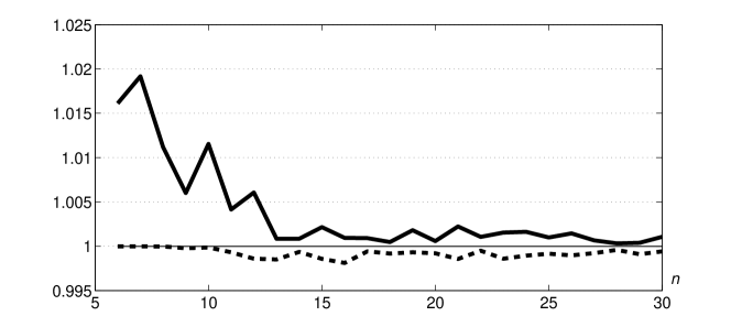
Figure 4: Upper bound (11) (thick solid line) and the value of the Wiener index for GreedyCaterpillar (dashed line) with respect to the Wiener index for the optimal caterpillar (thin horizontal line) vs graph order $n$

9 Conclusion

This article contributes to the literature on the Wiener index by studying the Wiener index maximization problem over the set $\mathcal{WT}(\mathbf{w},\mathbf{d})$ of trees with the given vertex weight sequence $\mathbf{w}$ and degree sequence $\mathbf{d}$. The results of [44] were extended to the Wiener index for graphs with weighted vertices: it was proven that if vertex weight sequence $\mathbf{w}$ is monotone in degree sequence $\mathbf{d}$, then there is an optimal caterpillar with internal/pendent vertex weights monotonously increasing from some central point to the ends of its backbone.

For weight sequences being monotone in degrees, closed-form expression (11) was proposed for the upper bound of the Wiener index value over $\mathcal{WT}(\mathbf{w},\mathbf{d})$. It was shown that this upper bound is tight, and an efficient greedy heuristics was proposed that approximates well the optimal tree. Finally, a branch and bound scheme was proposed for the exact solution of this NP-complete problem and computational analysis of its performance was accomplished.

Most of the results of this article are limited to the case of weight sequences being monotone in degrees, when the weight of an internal vertex does not decrease in its degree (no restrictions are imposed on weights of pendent vertices). The general case of non-monotonous weight sequences seems more complicated. Corollary 1 says that an optimal caterpillar exists, but weight sequences do not have to be V-shaped, so, expression (11) for the upper bound is directly inapplicable, although the solution of relaxed OCP (15), (17)-(21) still gives an efficiently calculable upper-bound estimate, and the greedy algorithm still builds some suboptimal trees.

References

• [1] A. A. Dobrynin, R. Entringer, I. Gutman, Wiener index of trees: theory and applications, Acta Appl. Math. 66 (3) (2001) 211–249. doi:10.1023/A:1010767517079.
• [2] H. Wang, The extremal values of the Wiener index of a tree with given degree sequence, Discrete App. Math. 156 (14) (2008) 2647–2654.
• [3] X.-D. Zhang, Q.-Y. Xiang, L.-Q. Xu, R.-Y. Pan, The Wiener index of trees with given degree sequences, MATCH Commun. Math. Comput. Chem. 60 (2) (2008) 623–644.
• [4] S. Klavžar, I. Gutman, Wiener number of vertex-weighted graphs and a chemical application, Discrete Appl. Math. 80 (1) (1997) 73–81.
• [5] A. Kelenc, S. Klavžar, N. Tratnik, The edge-Wiener index of benzenoid systems in linear time, MATCH Commun. Math. Comput. Chem. 74 (3) (2015) 521–532.
• [6] W. Gao, W. Wang, The vertex version of weighted Wiener number for bicyclic molecular structures, Comp. and Math. Meth. Med. 2015. doi:10.1155/2015/418106.
• [7] M. Goubko, O. Miloserdov, Simple alcohols with the lowest normal boiling point using topological indices, MATCH Commun. Math. Comput. Chem. 75 (2016) 29–56.
• [8] M. Goubko, Minimizing Wiener index for vertex-weighted trees with given weight and degree sequences, MATCH Commun. Math. Comput. Chem. 75 (2016) 3–27.
• [9] R. Shi, The average distance of trees, Sys. Sci. Math. Sci. 6 (1993) 18–24.
• [10] E. Çela, N. S. Schmuck, S. Wimer, G. J. Woeginger, The Wiener maximum quadratic assignment problem, Discrete Optim. 8 (3) (2011) 411–416.
• [11] H. Wiener, Structural determination of paraffin boiling points, J. Amer. Chem. Soc. 69 (1) (1947) 17–20.
• [12] M. Knor, R. Škrekovski, A. Tepeh, Mathematical aspects of Wiener index, Ars Math. Contemp. 11 (2) (2016) 327–352.
• [13] M. V. Diudea, I. Gutman, Wiener-type topological indices, Croatica Chem. Acta 71 (1) (1998) 21–51.
• [14] I. Gutman, Y.-N. Yeh, S.-L. Lee, Y.-L. Luo, Some recent results in the theory of the Wiener number, Indian J. Chem. 32 (1993) 651–661.
• [15] D. H. Rouvray, The modeling of chemical phenomena using topological indices, J. Comput. Chem. 8 (4) (1987) 470–480.
• [16] R. Lang, T. Li, D. Mo, Y. Shi, A novel method for analyzing inverse problem of topological indices of graphs using competitive agglomeration, Appl. Math. Comp. 291 (2016) 115–121. doi:10.1016/j.amc.2016.06.048.
• [17] M. Fischermann, A. Hoffmann, D. Rautenbach, L. Székely, L. Volkmann, Wiener index versus maximum degree in trees, Discrete Appl. Math. 122 (1) (2002) 127–137.
• [18] H. Lin, M. Song, On segment sequences and the Wiener index of trees, MATCH Commun. Math. Comput. Chem. 75 (1) (2016) 81–89.
• [19] H. Lin, Extremal Wiener index of trees with given number of vertices of even degree, MATCH Commun. Math. Comput. Chem. 72 (1) (2014) 311–320.
• [20] M. Krnc, R. Škrekovski, On Wiener inverse interval problem, MATCH Commun. Math. Comput. Chem. 75 (1) (2016) 71–80.
• [21] H. S. Ramane, V. V. Manjalapur, Note on the bounds on wiener number of a graph, MATCH Commun. Math. Comput. Chem. 76 (1) (2016) 19–22.
• [22] L. Shi, Chemical indices, mean distance, and radius, MATCH Commun. Math. Comput. Chem. 75 (1) (2016) 57–70.
• [23] R. Merris, An edge version of the matrix-tree theorem and the Wiener index, Linear Multilinear Algebra 25 (4) (1989) 291–296.
• [24] R. Merris, The distance spectrum of a tree, J. Graph Theory 14 (3) (1990) 365–369.
• [25] B. Mohar, Eigenvalues, diameter, and mean distance in graphs, Graphs and Combin. 7 (1) (1991) 53–64.
• [26] B. Mohar, The Laplacian spectrum of graphs, in: Y. Alavi, G. Chartrand, O. Ollermann, A. J. Schwenk (Eds.), Graph Theory, Combinatorics, and Applications, Vol. 2, Wiley, 1991, pp. 871–898.
• [27] G. Indulal, Sharp bounds on the distance spectral radius and the distance energy of graphs, Linear Algebra Appl. 430 (1) (2009) 106–113.
• [28] T. Gallai, P. Erdős, Graphs with prescribed degree of vertices (Hungarian), Mat. Lapok 11 (1960) 264–274.
• [29] S. A. Burr, P. Erdős, R. J. Faudree, A. Gyárfás, R. Schelp, Extremal problems for degree sequences, Combin. 52 (1988) 183–193.
• [30] T. Bıyıkoğlu, J. Leydold, Graphs with given degree sequence and maximal spectral radius, Electron. J. Combin. 15 (2008) R119.
• [31] I. Gutman, Degree-based topological indices, Croatica Chem. Acta 86 (4) (2013) 351–361.
• [32] I. Gutman, K. C. Das, The first Zagreb index 30 years after, MATCH Commun. Math. Comput. Chem. 50 (2004) 83–92.
• [33] I. Gutman, M. K. Jamil, N. Akhter, Graphs with fixed number of pendent vertices and minimal first Zagreb index, Trans. Combin. 4 (1) (2015) 43–48.
• [34] K. C. Das, K. Xu, J. Nam, Zagreb indices of graphs, Front. Math. China 10 (3) (2015) 567–582.
• [35] M. Ghorbani, M. A. Hosseinzadeh, A new version of Zagreb indices, Filomat 26 (1) (2012) 93–100.
• [36] M. Eliasi, A. Iranmanesh, I. Gutman, Multiplicative versions of first Zagreb index, MATCH Commun. Math. Comput. Chem. 68 (1) (2012) 217–230.
• [37] G. Fath-Tabar, Old and new Zagreb indices of graphs, MATCH Commun. Math. Comput. Chem. 65 (2011) 79–84.
• [38] K. Xu, K. C. Das, S. Balachandran, Maximizing the Zagreb indices of $(n,m)$-graphs, MATCH Commun. Math. Comput. Chem. 72 (2014) 641–654.
• [39] B. Furtula, I. Gutman, A forgotten topological index, J. Math. Chem. 53 (4) (2015) 1184–1190.
• [40] G. Su, J. Tu, K. C. Das, Graphs with fixed number of pendent vertices and minimal Zeroth-order general Randić index, Appl. Math. Comput. 270 (2015) 705–710.
• [41] K. Xu, H. Hua, A unified approach to extremal multiplicative Zagreb indices for trees, unicyclic and bicyclic graphs, MATCH Commun. Math. Comput. Chem. 68 (1) (2012) 241–256.
• [42] X.-D. Zhang, Extremal graph theory for degree sequences, arXiv preprint arXiv:1510.01903.
• [43] M. Liu, B. Liu, K. C. Das, Recent results on the majorization theory of graph spectrum and topological index theory, Electron. J. Lin. Algebra 30 (1) (2015) 402–421. doi:10.13001/1081-3810.3086.
• [44] N. S. Schmuck, S. G. Wagner, H. Wang, Greedy trees, caterpillars, and Wiener-type graph invariants, MATCH Commun. Math. Comput. Chem. 68 (1) (2012) 273–292.
• [45] I. Gutman, B. Furtula, M. Petrović, Terminal Wiener index, J. Math. Chem. 46 (2) (2009) 522–531.
• [46] I. Gutman, B. Furtula, A survey on terminal Wiener index, novel molecular structure descriptors – theory and applications i Edition, Univ. Kragujevac, Kragujevac, 2010, pp. 173–190.
• [47] B. Mohar, T. Pisanski, How to compute the Wiener index of a graph, J. Math. Chem. 2 (3) (1988) 267–277.
• [48] D. Spielman, Spectral graph theory, combin. sci. comp. Edition, CRC Press, Boca Raton, 2012, pp. 495–524.
• [49] D. A. Huffman, A method for the construction of minimum-redundancy codes, Proc. IRE 40 (9) (1952) 1098–1101.